Continuous Wavelet Transform and Back Propagation Neural Network for Condition Monitoring Chlorophyll Fluorescence Parameters Fv/Fm of Rice Leaves

Abstract

The chlorophyll fluorescence parameter Fv/Fm (maximum photosynthetic efficiency of optical system II) is an intrinsic index for exploring plant photosynthesis. Hyperspectral remote sensing technology can be used for rapid nondestructive detection of chlorophyll fluorescence parameters. Existing studies show that there is a good correlation between the vegetation index and Fv/Fm. However, due to the limited hyperspectral information reflected by the vegetation index, the established model often cannot reach the ideal accuracy. Therefore, this study took rice as the research object and explored the internal relationship between chlorophyll fluorescence parameters and spectral reflectance by setting different fertilization treatments. Spectral sensitive information was extracted by vegetation index and continuous wavelet transform (CWT) to explore a more suitable method for Fv/Fm hyperspectral estimation at the rice leaf scale. Then a monitoring model of Fv/Fm in rice leaves was established by the back propagation neural network (BPNN) algorithm. The results showed that: (1) the accuracy of univariate models constructed by Fv/Fm inversion based on 10 commonly used vegetation indices constructed by traditional methods was low; (2) The correlation between leaf hyperspectral reflectance and Fv/Fm could be effectively improved by using CWT, and the accuracy of the univariate model constructed by using the best wavelet coefficients could reach the level of rough evaluation of Fv/Fm; (3) The effect of wavelet transform using different mother wavelet functions as the basis function was different, and bior3.3 function was the best; R², RMSE and RPD of the BPNN model constructed by using the first 10 best wavelet coefficients decomposed by the bior3.3 was 0.823 6, 0.013 2 and 2.304 3. In conclusion, this study proves that CWT can effectively extract sensitive bands of rice leaves for Fv/Fm monitoring, providing a reference for the follow-up rapid and nondestructive monitoring of chlorophyll fluorescence.

1. Introduction

Photosynthesis is a critical component that influences crop growth and development, as well as the accumulation of material and yields. Chlorophyll fluorescence is known as the plant photosynthesis probe [1], and almost all changes in photosynthetic processes can be reflected by chlorophyll fluorescence [2]. The chlorophyll fluorescence parameter (Fv/Fm) is the maximum photosynthetic efficiency of optical system II reaction center [3], which is one of the most often utilized parameters, and it is widely employed in research on plant physiological changes and stressors [4,5,6]. It is critical to characterize the physiological status of plants by achieving quick nondestructive detection of Fv/Fm [7,8,9]. When using active fluorescence observation technology to directly measure chlorophyll fluorescence parameters, it usually requires a long-term dark reaction on the measured leaves, which cannot achieve real-time measurement and is not conducive to the monitoring of a large range of chlorophyll fluorescence parameters.

Hyperspectral remote sensing technology has the advantages of simplicity, sensitivity, and efficiency, and research on the use of hyperspectral data for monitoring plant physiological growth conditions has been developed in recent years [10,11,12,13,14]. Numerous studies on the link between plant chlorophyll fluorescence metrics and spectral features have been conducted. Zhang et al. [15] employed principal component analysis to identify the unique wavebands of rice leaf chlorophyll fluorescence parameters and then chose seven essential vegetation indices to model with fluorescence parameters. The results showed that the normalized difference spectral index (NDSI) constructed by 685 nm and 980 nm could be used for monitoring Fv/Fm, with a correlation coefficient of −0.818 and a root mean square error of 0.03. Tan et al. [16] investigated the association between the chlorophyll fluorescence parameter Fv/Fm and different hyperspectral vegetation indices in compact maize, and they discovered that the structure insensitive pigment index (SIPI) calculated at 445, 680, and 800 nm had the strongest correlation with Fv/Fm. By investigating the leaves of aspen and cherry trees, Peng et al. [17] discovered that the red edge normalized difference vegetation index (NDRE₇₄₀) and red edge chlorophyll index (CI₇₄₀) had the highest inversion accuracy for Fv/Fm, with R² exceeding 0.72 for both. El-Hendawy et al. [18] found that some vegetation indices based on water absorption spectral bands, chlorophyll spectral bands, and red edge spectral bands were more effective in estimating chlorophyll parameters than the photochemical vegetation index (PRI). According to Zheng et al. [19], the hyperspectral vegetation index D₆₉₀/D₁₃₂₀ based on the first-order differential spectrum had the highest accuracy with Fv/Fm, with a model coefficient of determination R² of 0.813 and RMSE of 0.042, after creating polynomial regressions of 13 new vegetation indices with chlorophyll fluorescence characteristics. The above studies show that it is possible to predict Fv/Fm by the reflection spectrum, but the current studies mainly establish the regression model through the vegetation index, and the method is relatively simple, so the prediction accuracy still has room for improvement.

Continuous wavelet transform (CWT) is a spectral analysis method that focuses on extracting spectral shape information, and it has powerful information processing and analysis capabilities [20]. It can decompose the spectrum at continuous wavelengths and scales, effectively weakening the negative effect of noise on the spectral information and highlighting the beneficial spectral information [21]. A back propagation neural network (BPNN), with self-learning, self-organization, self-adaptive capacity, and a highly nonlinear expression ability, may replicate the functioning of the human brain nervous system to some extent [22]. In the research of hyperspectral inversion, both the wavelet transform and the BP algorithm have been widely used in recent years [23,24,25,26,27,28,29]. Although some previous studies have used CWT to estimate crop agronomic parameters, it is still not enough to use CWT to highlight beneficial spectral information and then combine with machine learning algorithm inversion.

Rice (Oryza sativa L.) is one of the world’s most significant food crops [30], with more than half of the world’s population relying on it [31]. However, a study combining CWT with BPNN to invert the Fv/Fm of rice leaves has not yet been reported. Therefore, rice was selected as the research object and the objectives of this study were as follows: (1) retrieve the hyperspectral wavelength sensitive to the chlorophyll fluorescence parameters Fv/Fm of rice leaves using wavelet transform, (2) explore the best mother wavelet function and the best scale of fluorescence signal extraction, (3) compare the estimation accuracy of traditional regression models based on vegetation indices and wavelet parameters, (4) establish a BPNN based on vegetation indices and sensitive wavelet parameters for chlorophyll fluorescence parameters Fv/Fm of rice leaves. This work is expected to provide a reference for monitoring rice chlorophyll fluorescence parameters, using hyperspectral remote sensing technology.

2. Materials and Methods

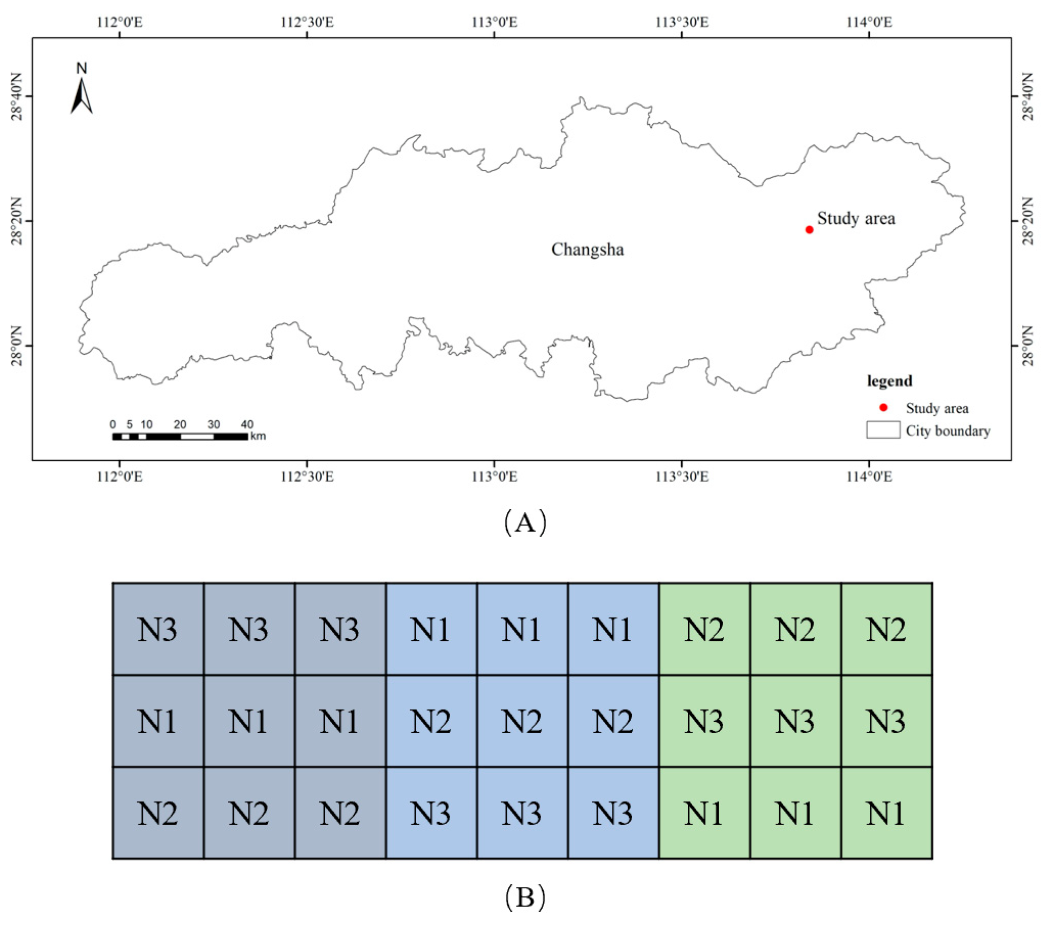
2.1. Experimental Design

The experiment was carried out at Hunan Agricultural University Liuyang Teaching and Research Base (113°84′ E, 28°30′ N) from May to September 2021, which is a small hilly basin with a humid subtropical monsoon climate, with an average annual temperature of 17.3 °C and average annual precipitation of 1358.6–1552.5 mm. The previous crop was rapeseed, and the soil organic matter, total N, total P, and total K contents were 23.41, 1.73, 0.64, and 19.35 g/kg⁻¹, respectively, and the pH was 5.51. The rice cultivar Jingliangyouhuazhan was the experimental material. Rice was sown on 14 May, planted on 16 May, transplanted on 4 June, and harvested on 15 September, with a total field growth period of 104 days. A mechanical seedling throwing technique was used in the experiment. The transplanting density was 22 cm × 25 cm, and three fertilizer conditions were set. The experiment was repeated 9 times with each plot area being 18 m² and randomly arranged. The geographical location of the test area and the specific test treatment scheme are shown in Figure 1 and

Table 1. Basic information of fertilizer treatment in the study area.

Treatments	Base Fertilizer (kg/hm2)		Tillering Fertilizer (kg/hm2)		Panicle Fertilizer (kg/hm2)
	15-15-15 Compound Fertilizer	Lime	15-15-15 Compound Fertilizer	Urea	15-15-15 Compound Fertilizer	KCI
N1	300	600	300	225	75	45
N2	300	600	150	150	75	45
N3	300	600	0	75	75	45

.

2.2. Data Acquisition

2.2.1. Measurement of Leaf Spectral Reflectance

The spectral reflectance of rice leaves was collected at 19, 33, 48, 64, 77, and 92 days after transplanting using a Field Spec 3 portable feature spectrometer (ASD, Boulder, CO, USA). The apparatus includes a hand-held leaf clip with a quartz halogenated light source and a reflected light-receiving probe inside the leaf clip that can be used to measure the living leaf. The spectral measurement range of the instrument is 350–2500 nm, where the spectral sampling interval of 350–1050 nm is 1.377 nm, the sampling interval of 1000–2500 nm is 2 nm, and the spectral resolution is 3 nm@700 nm, and 10 nm@1400 nm/2100 nm. Rice leaves with consistent growth were randomly selected from each plot for reflection spectroscopy. The reflectance spectral data of five leaves were collected in each plot, and the average value was taken as the final spectral value of the processing. By setting spectrum acquisition parameters, each spectral curve measured was resampled 10 times. Before and after each measurement, the standard whiteboard on the leaf clip was used for correction.

2.2.2. Measurement of Leaf Chlorophyll Fluorescence Parameters Fv/Fm

The chlorophyll fluorescence parameter Fv/Fm of rice leaves was measured by using a Flour Pen110 hand-held chlorophyll fluorimeter (PSI, Drásov, Czech Republic). Before the measurement, the leaves to be counted were clipped with dark adaptive leaf clips. After complete dark adaptation for 20 min, the chlorophyll fluorescence parameters Fv/Fm of the leaves at the same position as the reflectivity were measured by the instrument probe. Five leaves were measured in each treatment, and the average value was taken as the measured value of chlorophyll fluorescence Fv/Fm.

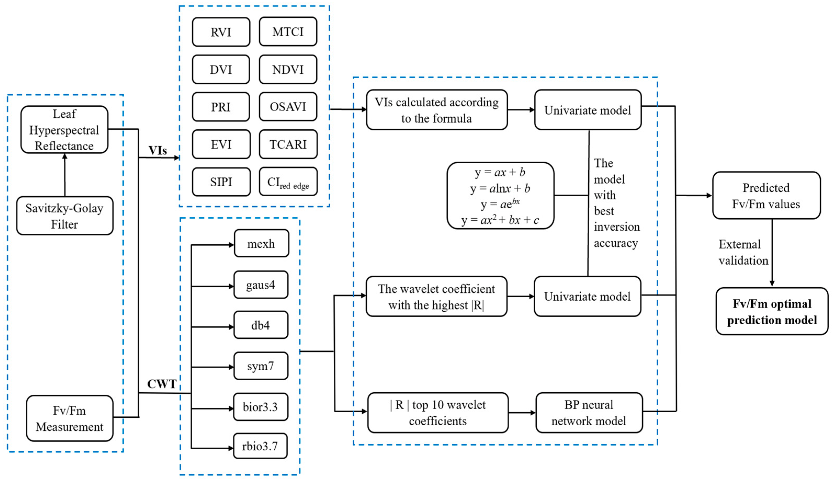
2.3. Data Processing and Analysis

The overall flow chart of data processing in this study is shown in Figure 2. It mainly includes the selection of the vegetation index, the selection of optimal wavelet basis function by CWT, and the establishment and verification of the Fv/Fm estimation model. All of the calculations were executed in MATLAB 2021b (MathWorks, Natick, MA, USA).

2.3.1. Measurement of Leaf Spectral Reflectance

Due to the large noise in the spectral range of 350–400 nm, considering the consistency of spectral resolution and according to previous studies [32,33,34,35], the visible and near-infrared range of the crop spectrum can reflect the growth status of crops, and wavelengths within the wavelength range of 400–1000 nm were selected for spectral analysis in this study. First, View Spec Pro 6.0 software (ASD, Boulder, CO, USA) was used to calculate the mean value of the original spectral data and export it. Then, the Sgolayfilt function was used to perform Savitzky–Golay smoothing and denoising. A total of 162 sets of data were measured in this experiment, and 159 sets of data were left after removing the samples with obvious spectral outliers. All data were sorted according to Fv/Fm from low to high, and one sample was selected in every two samples as a testing sample (53 samples in total), and the rest were selected as a training sample (106 samples in total). As shown in

Table 2. Statistical characteristics of Fv/Fm for all sample set, training set and test set.

Sample Set	Size	Max.	Min.	Mean	CV (%)
All	159	0.856 7	0.700 0	0.809 3	4.072 5
Training set	106	0.850 0	0.700 0	0.808 8	4.128 0
Testing set	53	0.856 7	0.710 0	0.810 2	3.957 0

, the mean value of Fv/Fm and coefficient of variation (CV) of the training set and test set have little difference, and the dispersion of samples is basically the same, so the samples of the training set and testing set have good representativeness.

2.3.2. Calculation of Vegetation Index

The vegetation index is derived by performing simple mathematical calculations on the reflectivity of different bands. Based on the spectral characteristics of rice and previous research results [16,36,37], in this study, 10 commonly used spectral indices were selected for the estimation of the chlorophyll fluorescence parameter Fv/Fm in rice leaves, and the specific calculation equations are shown in

Table 3. Vegetation index calculation formula.

Vegetation Index	Formula	Reference
Ratio Vegetation Index (RVI)	R685/R655	[38]
Difference Vegetation Index (DVI)	R800 − R675	[39]
Photochemical Reflectance Index (PRI)	(R531 − R570)/(R531 + R570)	[40]
Enhanced Vegetation Index (EVI)	2.5 × (R810 − R690)/(R810 + 2.4 × R690 + 1)	[41]
Structure Insensitive Pigment Index (SIPI)	(R800 − R445)/(R800 − R680)	[42]
MERIS terrestrial chlorophyll Index (MTCI)	(R750 − R710)/(R710 − R680)	[43]
Normalized Difference Vegetation Index (NDVI)	(R800 − R670)/(R800 + R670)	[44]
Optimization Soil-Adjusted Vegetation Index (OSAVI)	1.16 × (R800 − R670)/(R800 + R670 + 0.16)	[45]
Transformed Chlorophyll Absorption in Reflectance Index (TCARI)	3 × [(R700 − R670) − 0.2 × (R700 − R550) × (R700/R670)]	[46]
Red edge chlorophyll index (CIred edge)	(R800/R720) − 1	[47,48]

.

2.3.3. Continuous Wavelet Transform

Wavelet transformation is a linear transformation method first proposed by MORLET, a French engineer. This method can decompose complex signals into wavelet signals of different scales (frequencies), can effectively extract the weak information part of the signal, fully highlight local characteristics, and has the characteristics of multi-resolution analysis. Continuous wavelet transform (CWT) is a type of wavelet transform that can realize signal transformation and signal reconstruction, maintain the integrity of the original information, and have reversibility [49]. In this study, CWT is used to decompose the original hyperspectral reflectance through the wavelet basis function, and a series of wavelet coefficients (WCs) at different scales are obtained. WCs contain two dimensions, which are spectral bands (I = 1, 2, 3, …, m) and decomposition scales (j = 1, 2, …, n). Therefore, CWT transforms the original one-dimensional hyperspectral data into a two-dimensional matrix of WCs, which is composed of spectral bands and decomposition scales. Its transformation formula is as follows:

$$\left\{\begin{array}{c}{W}_f\left(a,b\right)\le f\\ {\psi }_{a,b}\left(\lambda \right)\ge {{\displaystyle \int }}_{-\infty }^{+\infty }f\left(\lambda \right){\psi }_{a,b}\left(\lambda \right)d\lambda \end{array}\right.$$

(1)

$${\psi }_{a,b}\left(\lambda \right)=\frac{1}{\sqrt{a}}\psi \left(\frac{\lambda -b}{a}\right)$$

(2)

where λ is the number of spectral bands; a is the scale factor; b is the translation factor; $f\left(\lambda \right)$ is the spectral reflectance of leaves; ${\psi }_{a,b}$ is the wavelet basis function; and $W_f\left(a,b\right)$ is the wavelet coefficient. Since the dimensionality reduction effect of different wavelet basis functions is different, according to previous studies [22,23,24,50], different mother wavelet functions were applied in this study to process hyperspectral data. Finally, we selected six mother wavelet functions, mexh, guas4, db4, sym7, bior3.3, and rbio3.7, as the basis functions of the process of CWT, and the decomposition scales were set as 2¹, 2², …, 2¹⁰, corresponding to scales 1–10.

2.3.4. Back Propagation Neural Network

The back propagation neural network (BPNN) is a kind of multilayer feedforward neural network trained according to the error back propagation algorithm, which is one of the most widely used neural network models. The structure of the BPNN usually includes an input layer hidden layer and an output layer. In this study, the BPNN model was trained by MATLAB 2021b programming. To make the network easily converge in the training stage, input and output variables were normalized. The transfer function of neurons in the middle layer of the network adopts the s-type tangent function Tansig, the transfer function of neurons in the output layer adopts the linear function Purelin, and the training function of the network adopts the Levenberg–Marquardt algorithm training function Trainlm, and the learning function is learngdm. The number of iterations of network training is 1000, the minimum error of the training target is 10⁻⁶, and the learning rate is 0.01. The number of hidden layer nodes is determined by formula (3) and the grid search algorithm.

$$q=\sqrt{k+m}+\alpha$$

(3)

where k is the number of input layer element variables; m is the output layer element and α is in [1,10].

2.4. Evaluation of Model Accuracy

The coefficient of determination (R²), root mean square error (RMSE), and relative analysis error (RPD) were used to evaluate the model accuracy. The value of R² is between 0 and 1. The closer R² is to 1, the smaller RMSE is, indicating that the model fitting effect is better and the prediction accuracy is higher. When RPD < 1.4, the model could not predict the samples; at 1.4 ≤ RPD < 2, the sample can be roughly evaluated; and when RPD ≥ 2, the model has excellent predictive ability. The calculation formulas of R², RMSE, and RPD are as follows:

$$R^2=1-\frac{{{\displaystyle \sum }}_{i=1}^n{\left(y_i-y_j\right)}^2}{{{\displaystyle \sum }}_{i=1}^n{\left(y_i-\overline{y}\right)}^2}$$

(4)

$$RMSE=\sqrt{\frac{{{\displaystyle \sum }}_{i=1}^n{\left(y_i-y_j\right)}^2}{n}}$$

(5)

$$RPD=\frac{St{d}_v}{RMS{E}_v}$$

(6)

where y_i is the measured value, y_j is the predicted value, $\overline{y}$ is the average value, Std_v is the standard deviation of the testing set, RMSE_v is the RMSE of the testing set, and n is the number of samples.

3. Results

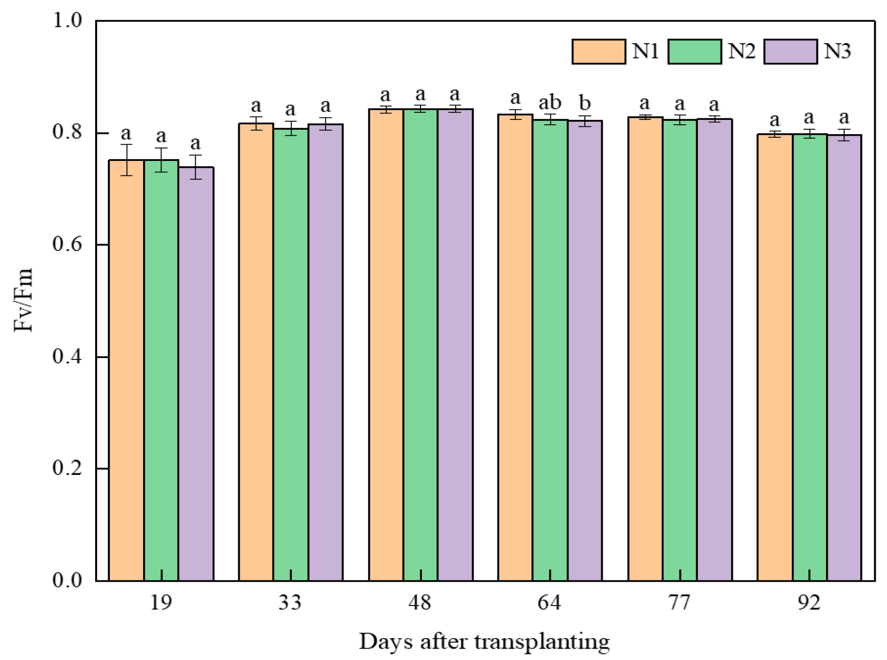
3.1. Dynamic Changes of Fv/Fm under Different Treatments

Figure 3 shows the dynamic changes in Fv/Fm in rice leaves under different treatments. From the perspective of the number of days after rice transplanting, Fv/Fm under different fertilization conditions showed the same overall pattern, that is, with the advance of rice growth, Fv/Fm showed a trend of first increasing and then decreasing, reaching the maximum at 48 days after rice transplanting, then gradually decreasing, but it appeared to temporarily rise at 77 days after rice transplanting. From the perspective of different fertilization levels, at 64 days after transplanting, reduced fertilization significantly reduced the Fv/Fm of rice leaves, and the decrease in Fv/Fm in the N3 treatment was 1.4% compared with that in the N1 treatment.

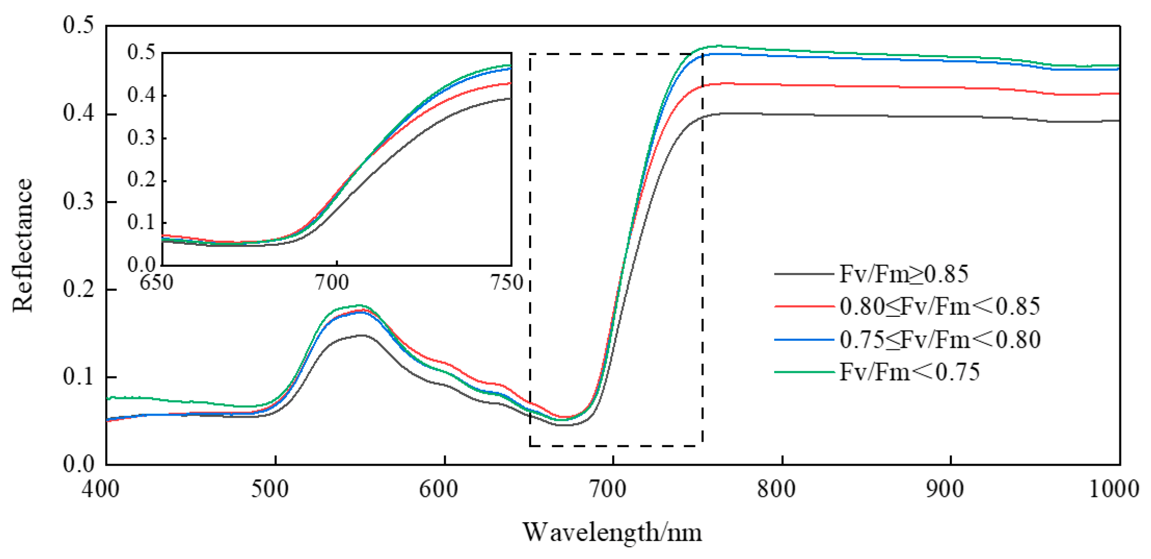
3.2. Original Spectral Reflectance at Different Fv/Fm Intervals

The Fv/Fm values of the leaf samples were divided into four intervals according to a step size of 0.05 [51], and the reflection spectra of rice leaves corresponding to Fv/Fm values in each interval were averaged, as shown in Figure 4. The spectral reflectance of rice leaves conforms to the general rule of the plant spectrum, and it is affected by the content of pigment and nitrogen in leaves and the internal structure of leaves (leaf gap and cell thickness). The spectrum of rice leaves forms two absorption valleys (“blue valley” and “red valley”) and one reflection peak (“green peak”) in the visible band. The phenomenon of “red edge” with a sharp rise of reflectivity appears between visible and near-infrared bands. A high reflectivity platform “red shoulder” appears in the near-infrared band. The spectral reflectance of rice leaves in different intervals of Fv/Fm showed roughly the same change law, but there were also obvious differences, namely, with the increase in leaf Fv/Fm, the overall spectral reflectance showed a downward trend. The decrease in spectral reflectance in the 500–700 nm region reflected this trend very obviously. In the red-edged area, with the decrease in Fv/Fm, the slope of spectral reflectance increases obviously.

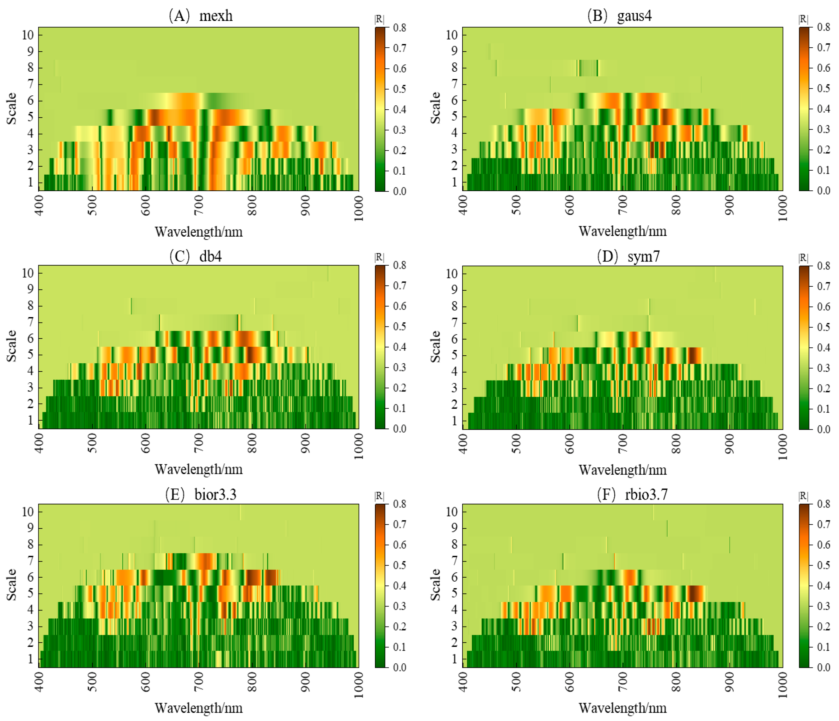
3.3. Correlation of Wavelet Coefficients with Fv/Fm

The spectral reflectance data of rice leaves were decomposed at scales of 1 to 10 by CWT, and the corresponding wavelet coefficients were generated for each band under each decomposition scale. Correlation analysis was performed between wavelet coefficients and Fv/Fm at each scale, and the |R| between wavelet coefficients and Fv/Fm at each scale was calculated. All calculated |R| at each scale was constructed into a 601 × 10 matrix, the abscissa corresponding to each pixel in the matrix was the original spectral band (400–1000 nm), and the ordinate was the decomposition scale (1–10). Each pixel was the wavelet coefficient of CWT in different wavelength bands and different decomposition scales, and the chromaticity value of each pixel represented the |R| of wavelet coefficients and Fv/Fm generated by CWT. Since six different mother wavelet functions were used as the basis functions of CWT in this study, a total of six |R| matrix plots were obtained (Figure 5). As shown in Figure 5, the bands with a stronger correlation were distributed in both the visible and near-infrared regions. From different scales, the regions with a high correlation between the spectrum and Fv/Fm after CWT decomposition under 6 different mother wavelet functions were concentrated in the 3–6 scale, and the band with the highest coefficient of determination and its scale is shown in

Table 4. |R| of Fv/Fm with WCs.

Mother Wavelet Functions	mexh	gasu4	db4	sym7	bior3.3	rbio3.7
Wavelength (nm)	644	756	795	828	794	830
Scale	4	3	5	5	6	5
|R|	0.776 3 **	0.793 9 **	0.769 2 **	0.783 6 **	0.780 0 **	0.799 7 **

** indicates significant correlation at the 0.01 probability level.

.

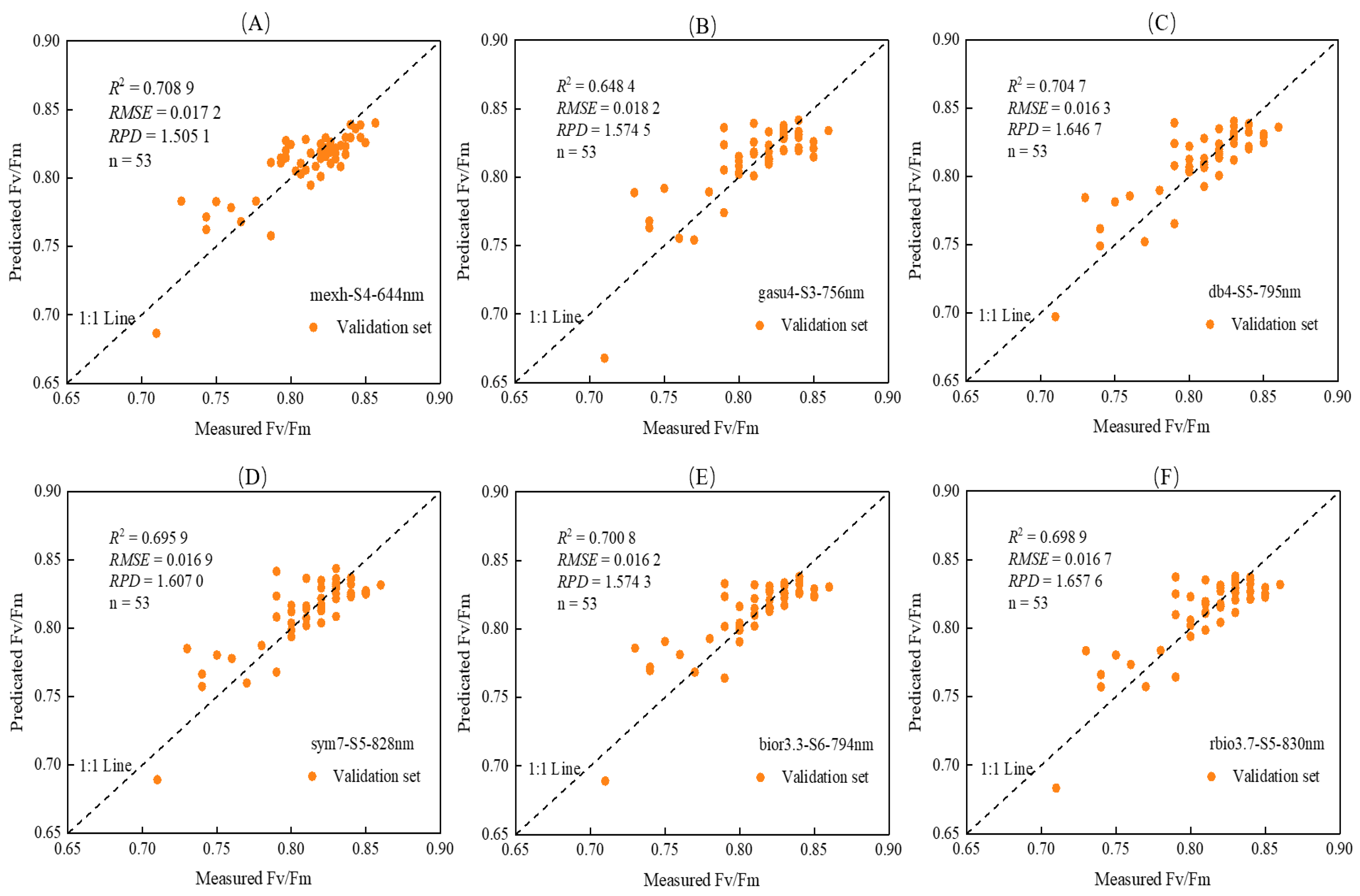
3.4. Single-Index Traditional Leaf Fv/Fm Estimation Models

The spectral vegetation indices calculated by formulas and the wavelet coefficient with the highest |R| selected after CWT decomposition (under different mother wavelet functions) were used as independent variables and Fv/Fm as dependent variables, respectively, and four univariate linear or nonlinear fitting models were commonly used for model construction: the linear function y = ax + b; the logarithmic function y = alnx + b; the exponential function y = ae^bx; and the quadratic function y = ax² + bx + c. For each independent variable, the regression equation with the best inversion accuracy was selected for training (n = 106), and the testing set (n = 53) data were used for external verification.

According to

Table 5. Performance of models for estimating Fv/Fm based on VIs and wavelet features.

Indices	Equation	Training Set		Testing Set
		RC2	RMSEC	RV2	RMSEV	RPD
RVI	y = −2.316 9x2 + 5.271 2x – 2.164 9	0.597 4	0.020 4	0.517 2	0.020 3	1.002 0
DVI	y = 0.007 2x2 + 0.687x + 0.5311	0.420 4	0.025 2	0.360 5	0.024 9	0.840 8
PRI	y = 22.576x2 − 1.095 4x + 0.793 5	0.291 9	0.026 3	0.219 5	0.027 6	0.691 8
EVI	y = 0.459 4x2 − 0.104 7x + 0.720 3	0.238 9	0.027 4	0.188 5	0.026 6	0.529 7
SIPI	y = −0.622 6x2 + 1.306 2x + 0.125 9	0.048 3	0.032 5	0.001 1	0.031 6	0.051 1
MTCI	y= −0.013 3x2 + 0.026 6x + 0.796 3	0.001 1	0.032 2	0.000 2	0.031 4	0.028 6
NDVI	y = 6.200 3x2 − 9.070 2x + 4.098 1	0.119 9	0.029 3	0.064 7	0.028 2	0.455 2
OSAVI	y = 1.180 7x2 + 0.440 1x + 0.5629	0.435 3	0.024 3	0.355 1	0.025 0	0.846 9
TCARI	y = −1.498 7x2 + 1.180 8x + 0.587 4	0.141 2	0.029 9	0.193 3	0.029 3	0.360 3
CIred edge	y = −0.278 9x2 + 0.166 4x + 0.787 1	0.016 6	0.032 2	0.009 6	0.031 4	0.069 7
mexh-S4-644nm	y = −50.573x2 − 6.036 7x + 0.686 6	0.614 3	0.020 3	0.708 9	0.017 2	1.505 1
gasu4-S3-756nm	y = −54 283x2 − 222.45x + 0.667 9	0.638 1	0.019 5	0.648 4	0.018 2	1.574 5
db4-S5-795nm	y = 330.14x2 − 0.550 5x + 0.697 3	0.647 1	0.019 4	0.704 7	0.016 3	1.646 7
sym7-S5-828nm	y = 10.462x2 + 27.951x + 0.693	0.630 1	0.020 3	0.695 9	0.016 9	1.607 0
bior3.3-S6-794nm	y = −130.89x2 − 9.868 9x + 0.689 1	0.616 8	0.020 5	0.700 8	0.016 2	1.574 3
rbio3.7-S5-830nm	y = 2017.1x2 + 29.21x + 0.683 3	0.642 4	0.020 0	0.698 9	0.016 7	1.657 6

, the equation with the best inversion accuracy for each parameter was the quadratic equation, and the R² of the training set sample Fv/Fm estimation model ranged from 0.001 1 to 0.647 1. Through the verification of the estimated model, it can be found that the model based on a single spectral index had a low fitting effect and prediction accuracy, and the stability was poor. The R² of both the training set samples and the testing set samples reached above 0.6 for the models constructed based on the wavelet coefficients, and the RPDs of the testing set models were both greater than 1.4 (Figure 6). Among them, the Fv/Fm estimation model y = 330.14x² − 0.550 5x + 0.697 3 constructed with the wavelet coefficient at db4 (795 nm, Scale 5) as the independent variable worked best and had the highest accuracy, with testing sets R², RMSE, and RPD of 0.704 7, 0.016 3 and 1.646 7, respectively.

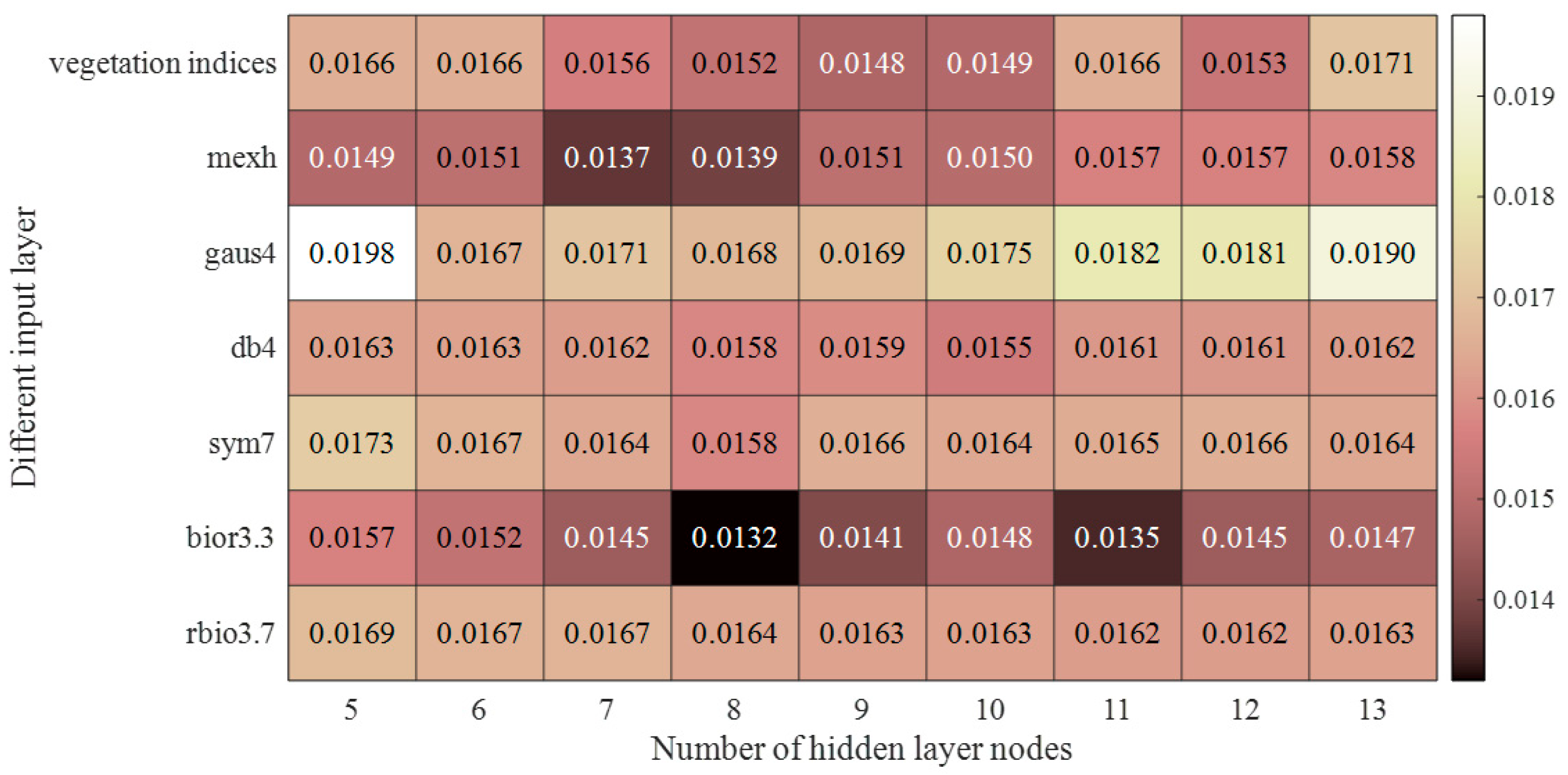
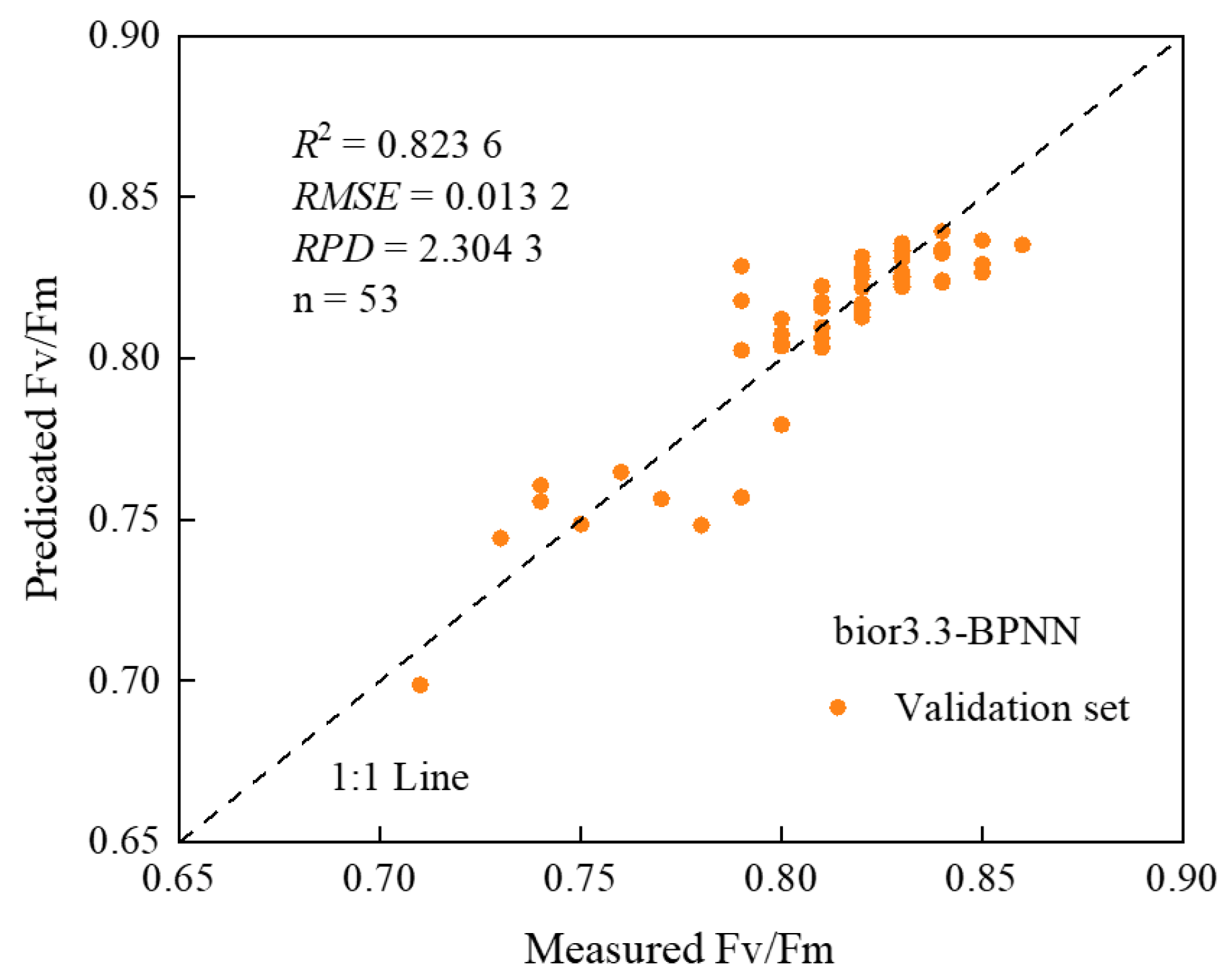
3.5. Models for Monitoring the Leaf Fv/Fm Based on BPNN

According to the results of CWT in Figure 5, 10 vegetation indices and the 10 bands with the highest |R| under each mother wavelet function (

Table 6. The top 10 sensitive bands under different mother wavelet functions.

Mother Vavelet Functions	Scale	Wavelength (nm)
mexh	scale4	643, 644, 645
	scale5	614, 615, 616, 617, 618, 619, 620
gasu4	scale3	754, 755, 756, 757, 773, 774, 775
	scale5	777, 778, 779
db4	scale3	760, 761
	scale5	792, 793, 794, 795, 796, 797, 798, 799
sym7	scale5	785, 826,827, 828, 829, 839, 831, 832, 833, 834
bior3.3	scale4	749
	scale6	792, 793, 794, 795, 796, 797, 831, 832, 833
rbio3.7	scale3	749, 750
	scale5	827, 828, 829, 830, 831, 832, 833, 834

) were selected as sensitive bands, and the wavelet coefficients corresponding to them were used as the input layer of the BP neural network, The Fv/Fm of rice leaves was used as the output layer to construct BP neural network models individually, and the results are shown in Figure 7 and

Table 7. Fv/Fm estimation model based on CWT and BPNN.

WCs	BP Neural Network Architecture	Training Set		Testing Set
		RC2	RMSEC	RV2	RMSEV	RPD
Vegetation indices	10-9-1	0.813 5	0.014 0	0.766 4	0.014 8	1.743 4
mexh	10-7-1	0.804 4	0.014 2	0.795 8	0.013 7	2.165 3
gaus4	10-6-1	0.816 0	0.013 9	0.730 5	0.016 7	1.717 4
db4	10-10-1	0.811 4	0.014 0	0.746 5	0.015 5	2.029 4
sym7	10-8-1	0.818 3	0.014 2	0.734 7	0.015 8	1.860 4
bior3.3	10-8-1	0.822 3	0.014 0	0.823 6	0.013 2	2.304 3
rbio3.7	10-11-1	0.796 6	0.014 9	0.723 3	0.016 2	1.978 8

. As shown in Figure 7, the number of different hidden layers had a significant influence on the accuracy of the model and every neural network had an optimal number of hidden layer nodes. The fitting effect and prediction accuracy of the model constructed by the BPNN were improved compared with those of the univariate model, which was due to the stronger nonlinear fitting ability of machine learning.

The wavelet coefficients calculated by vegetation indices, mexh, gaus4, db4, sym7, and rbio3.7 as the mother wavelet function were used as the input layer, and the BPNN model constructed had the phenomenon of overfitting, namely, the accuracy of the training set was significantly higher than that of the testing set. Taking the wavelet coefficients calculated by bior3.3 as the mother wavelet function as the input layer, the BPNN model with the 10-8-1 architecture had the best effect and good generalization ability. Its testing set R² was 0.823 6, RMSE was 0.013 2, and the RPD was 2.304 3, as shown in Figure 8.

4. Discussion

Chlorophyll fluorescence signals emitted by plants contain abundant information about photosynthesis, and chlorophyll fluorescence parameters are internal indicators that relate plant photosynthesis to the external environment [52]. Under normal conditions, the chlorophyll fluorescence parameter Fv/Fm of leaves remains unchanged for different species and ecotypes [53]. Studies have shown that chlorophyll fluorescence, a natural probe emitted by plants, can effectively detect much information about plant growth and nutrition [54,55]. Fertilization can supplement and distribute the nutrients required for plant growth and development. Fertilizer levels influence rice growth and development, which in turn influences the Fv/Fm of rice leaves. In this study, 64 days after transplanting, different fertilizer treatments of Fv/Fm showed a significant difference between the N3 treatment under Fv/Fm significantly below N1, which could be due to reducing fertilization, nutrient supply, nutrient deficiency, and underlying causes of optical system II active center damage to some extent, thus reducing leaf photosynthetic activity. However, the difference between the N1 and N2 treatments was not statistically significant, indicating that more research is required to determine the precise mechanism of the effect of fertilizer conditions on rice photosynthetic characteristics.

The differences in spectral characteristics of crop leaves reflect the growth and development of crops and their nutritional status [56]. Fv/Fm is a characterization of the maximum photochemical efficiency or primary light energy conversion efficiency of photosystem II (PS II), which reflects the ability of plant leaves to absorb light energy. As a result, when the Fv/Fm value was high, the absorption capacity was enhanced, and the reflectivity decreased; when the Fv/Fm value decreased, the reflectivity increased. This provides a theoretical basis for the hyperspectral inversion of Fv/Fm [43]. Most studies [15,16,17,18,19] use the vegetation index construction method to remove noise existing in the original spectral information and mine sensitive parameter information. In this study, we selected the RVI, DVI, PRI, EVI, SIPI, MICI, NDVI, OSAVI, TCARI, and CIred edge to estimate the Fv/Fm of rice leaves by establishing a single vegetation index estimation model. The results showed that the training set accuracy and testing set accuracy could not reach the degree of effective estimation at the same time. This may be because the ability of the conventional vegetation index to correct spectral reflectance is easily interfered with by external factors, and the spectral information it reflects is very limited. Therefore, it is easy to cause a poor prediction effect of Fv/Fm.

As a spectral data processing method, CWT can well mine weak and effective spectral information, which is of great significance in the inversion of crop growth parameters [57] and has also been used to monitor the kinetic parameters of chlorophyll fluorescence. Zhao et al. [23] combined the CWT and RF algorithms, and the monitoring modeling of potato leaf Fv/Fm values showed that bior3.3-RF-PLS had the best monitoring performance. Jia et al. [24] investigated wheat leaves and discovered that linear models built from wavelet-based REP (WREP-S4) and wavelet features (704 nm, scale 4) outperformed other spectral features in calibration and validation datasets. In the study of Fv/Fm estimation using CWT, the choice of a mother wavelet function and the most appropriate decomposition scale are not sufficient. There are also great differences in the ability of different types of mother wavelet functions to describe local features of spectral signals. Therefore, six kinds of mother wavelet functions were selected as the basis functions of CWT. The results showed that the bands with a high correlation between wavelet coefficients and Fv/Fm were mostly in the range of 700~850 nm after using different mother wavelet functions for wavelet transform, and the decomposition scales were all in the optimal scale of scale 3 to scale 6 (Figure 5). The accuracy of the Fv/Fm estimation model constructed by using the obtained wavelet coefficients was significantly improved compared with the model constructed by the vegetation index. The RPDs of the univariate Fv/Fm estimation model based on the optimal wavelet coefficients and the BPNN model based on the first 10 sensitive wavelet coefficients both reach the level of rough evaluation of the model. Meanwhile, the RPD of the BPNN model was higher than that of the univariate model, which indicated that the monitoring performance of the Fv/Fm estimation model could be optimized through the machine learning algorithm. However, only the mexh-BPNN (10-7-1), db4-BPNN (10-10-1), and bior3.3-BPNN (10-8-1) models had high reliability and could be used for model analysis, among which the bior3.3-BPNN (10-8-1) model had the best monitoring performance.

The results of this study are obtained on the basis of the comprehensive analysis of data from different fertilization treatments and different growth periods, which have certain universality, but there are still some shortcomings. In this study, the spectral information at the leaf scale of rice was decomposed, while the spectral information at the canopy scale of rice was more affected by environmental background noise, such as soil and water, so whether the spectral information decomposition through CWT can help highlight the beneficial spectral information of the canopy remains to be discussed. When selecting sensitive hyperspectral information to build a model, it is still limited to use the parameters corresponding to high correlation coefficients. This is because how the characteristic variables are selected from the redundant and complex variables can directly determine the performance of the prediction model. In this paper we only use the BP neural network, while there are many other methods of machine learning to establish the predicting model. At the same time, because the experimental data used in this study are only one year, the results still need to be verified and improved in different field environments. In future studies, long-term localization experiments should be carried out, and the diversity of germplasm resources of experimental materials should be increased. Meanwhile, studies of different scales should be carried out to accumulate experimental data. It is also necessary to study the Fv/Fm monitoring optimization algorithm and analyze the influence of other factors on Fv/Fm hyperspectral monitoring to establish a more stable Fv/Fm hyperspectral monitoring model.

5. Conclusions

In this study, the Fv/Fm of rice leaves under different fertilization conditions had the same change pattern with the advancement of the growth period, and the difference between treatments reached a significant level 64 days after transplanting. To monitor the chlorophyll fluorescence parameter (Fv/Fm) of rice leaves, we used 10 types of vegetation indices and CWT to extract effective information from the original hyperspectral data of rice leaves. By comparing them, we found that bior3.3-BPNN (10-8-1) model constructed by using bior3.3 as the basis function to decompose the original spectral data combined with the BP neural network algorithm has a high prediction accuracy, with an R² of 0.823 6, RMSE was 0.013 2, and the RPD was 2.304 3 of the testing set. This study is helpful to advance the application of CWT and BPNN in chlorophyll fluorescence parameter inversion.

References

1. Bussotti, F.; Gerosa, G.; Digrado, A.; Pollastrini, M. Selection of chlorophyll fluorescence parameters as indicators of photosynthetic efficiency in large scale plant ecological studies. Ecol. Indic. 2020, 108, 105686. [Google Scholar] [CrossRef]
2. Hikosaka, K.; Tsujimoto, K. Linking remote sensing parameters to CO2 assimilation rates at a leaf scale. J. Plant Res. 2021, 134, 695–711. [Google Scholar] [CrossRef] [PubMed]
3. Butler, W.L.; Kitajima, M. Fluorescence quenching in photosystem II of chloroplasts. Biochim. Biophys. Acta 1975, 376, 116–125. [Google Scholar] [CrossRef]
4. Buschmann, C.; Schweiger, J.; Lichtenthaler, H.K.; Richter, P. Application of the Karlsruhe CCD-OMA LIDAR-fluorosensor in stress detection of plants. J. Plant Physiol. 1996, 148, 548–554. [Google Scholar] [CrossRef]
5. Ciompi, S.; Gentili, E.; Guidi, L.; Soldatini, G.F. The effect of nitrogen deficiency on leaf gas exchange and chlorophyll fluorescence parameters in sunflower. Plant Sci. 1996, 118, 177–184. [Google Scholar] [CrossRef]
6. Mallick, N.; Mohn, F.H. Use of chlorophyll fluorescence in metal-stress research: A case study with the green microalga Scenedesmus. Ecotox. Environ. Safe 2003, 55, 64–69. [Google Scholar] [CrossRef]
7. Sun, H.; Liu, W.; Wang, Y.; Yuan, S. Evaluation of Typical Spectral Vegetation Indices for Drought Monitoring in Cropland of the North China Plain. IEEE J. Sel. Top. Appl. Earth Observ. Remote Sens. 2017, 10, 5404–5411. [Google Scholar] [CrossRef]
8. Fusaro, L.; Salvatori, E.; Mereu, S.; Manes, F. Photosynthetic traits as indicators for phenotyping urban and peri-urban forests: A case study in the metropolitan city of Rome. Ecol. Indic. 2019, 103, 301–311. [Google Scholar] [CrossRef]
9. Sayed, O.H. Chlorophyll Fluorescence as a Tool in Cereal Crop Research. Photosynthetica 2003, 41, 321–330. [Google Scholar] [CrossRef]
10. Gitelson, A.A.; Zur, Y.; Chivkunova, O.B.; Merzlyak, M.N. Assessing Carotenoid Content in Plant Leaves with Reflectance Spectroscopy. Photochem. Photobiol. 2002, 75, 272–281. [Google Scholar] [CrossRef]
11. Guo, B.B.; Qi, S.L.; Heng, Y.R.; Duan, J.Z.; Zhang, H.Y.; Wu, Y.P.; Feng, W.; Xie, Y.X.; Zhu, Y.J. Remotely assessing leaf N uptake in winter wheat based on canopy hyperspectral red-edge absorption. Eur. J. Agron. 2017, 82, 113–124. [Google Scholar] [CrossRef]
12. Liang, L.; Qin, Z.H.; Zhao, S.H.; Di, L.P.; Zhang, C.; Deng, M.X.; Lin, H.; Zhang, L.P.; Wang, L.J.; Liu, Z.X. Estimating crop chlorophyll content with hyperspectral vegetation indices and the hybrid inversion method. Int. J. Remote Sens. 2016, 37, 2923–2949. [Google Scholar] [CrossRef]
13. Guo, C.F.; Xiao, Y. Estimating leaf chlorophyll and nitrogen content of wetland emergent plants using hyperspectral data in the visible domain. Spectr. Lett. 2016, 49, 180–187. [Google Scholar] [CrossRef]
14. Steidle Neto, A.J.; Lopes, D.C.; Pinto, F.A.C.; Zolnier, S. Vis/NIR spectroscopy and chemometrics for nondestructive estimation of water and chlorophyll status in sunflower leaves. Biosyst. Eng. 2017, 155, 124–133. [Google Scholar] [CrossRef]
15. Zhang, H.; Zhu, L.F.; Hu, H.; Zheng, K.F.; Jin, Q.Y. Monitoring leaf chlorophyll fluorescence with spectral reflectance in Rice (Oryza sativa L.). Procedia Eng. 2011, 15, 4403–4408. [Google Scholar] [CrossRef] [Green Version]
16. Tan, C.W.; Huang, W.J.; Jin, X.L.; Wang, J.C.; Tong, L.; Wang, J.H.; Guo, W.S. Using Hyperspectral Vegetation Index to Monitor the Chlorophyll Fluorescence Parameters Fv/Fm of Compact Corn. Guang Pu Xue Guang Pu Fen Xi 2012, 32, 1287–1291. [Google Scholar] [CrossRef]
17. Peng, Y.; Zeng, A.L.; Zhu, T.; Fang, S.H.; Gong, Y.; Tao, Y.Q.; Zhou, Y.; Liu, K. Using remotely sensed spectral reflectance to indicate leaf photosynthetic efficiency derived from active fluorescence measurements. J. Appl. Remote Sens. 2017, 11, 026034. [Google Scholar] [CrossRef] [Green Version]
18. El-Hendawy, S.; Al-Suhaibani, N.; Elsayed, S.; Alotaibi, M.; Hassan, W.; Schmidhalter, U. Performance of optimized hyperspectral reflectance indices and partial least squares regression for estimating the chlorophyll fluorescence and grain yield of wheat grown in simulated saline field conditions. Plant Physiol. Biochem. 2019, 144, 300–311. [Google Scholar] [CrossRef]
19. Zheng, W.; Lu, X.; Li, Y.; Li, S.; Zhang, Y. Hyperspectral Identification of Chlorophyll Fluorescence Parameters of Suaeda salsa in Coastal Wetlands. Remote Sens. 2021, 13, 2066. [Google Scholar] [CrossRef]
20. Rivard, B.; Feng, J.; Gallie, A.; Sanchez-Azofeifa, A. Continuous wavelets for the improved use of spectral libraries and hyperspectral data. Remote Sens. Environ. 2008, 112, 2850–2862. [Google Scholar] [CrossRef]
21. Blackburn, G.A.; Ferwerda, J.G. Retrieval of chlorophyll concentration from leaf reflectance spectra using wavelet analysis. Remote Sens. Environ. 2008, 112, 1614–1632. [Google Scholar] [CrossRef]
22. Keiner, L.E.; Yan, X.H. A Neural Network Model for Estimating Sea Surface Chlorophyll and Sediments from Thematic Mapper Imagery. Remote Sens. Environ. 1998, 66, 153–165. [Google Scholar] [CrossRef]
23. Le Maire, G.; François, C.; Dufrêne, E. Towards universal broad leaf chlorophyll indices using PROSPECT simulated database and hyperspectral reflectance measurements. Remote Sens. Environ. 2004, 89, 1–28. [Google Scholar] [CrossRef]
24. Zhao, R.; An, L.; Song, D.; Li, M.; Qiao, L.; Liu, N.; Sun, H. Detection of chlorophyll fluorescence parameters of potato leaves based on continuous wavelet transform and spectral analysis. Spectroc. Acta Pt. A Molec. Biomolec. Spectr. 2021, 259, 119768. [Google Scholar] [CrossRef]
25. Jia, M.; Li, D.; Colombo, R.; Wang, Y.; Wang, X.; Cheng, T.; Zhu, Y.; Yao, X.; Xu, C.; Ouer, G.; et al. Quantifying Chlorophyll Fluorescence Parameters from Hyperspectral Reflectance at the Leaf Scale under Various Nitrogen Treatment Regimes in Winter Wheat. Remote Sens. 2019, 11, 2838. [Google Scholar] [CrossRef] [Green Version]
26. Chen, L.; Huang, J.F.; Wang, F.M.; Tang, Y.L. Comparison between back propagation neural network and regression models for the estimation of pigment content in rice leaves and panicles using hyperspectral data. Int. J. Remote Sens. 2007, 28, 3457–3478. [Google Scholar] [CrossRef]
27. Kira, O.; Linker, R.; Gitelson, A. Nondestructive estimation of foliar chlorophyll and carotenoid contents: Focus on informative spectral bands. Int. J. Appl. Earth Obs. Geoinf. 2015, 38, 251–260. [Google Scholar] [CrossRef]
28. Sabanci, K.; Aslan, M.F.; Durdu, A. Bread and Durum Wheat Classification Using Wavelet Based Image Fusion. J. Sci. Food Agric. 2020, 100, 5577–5585. [Google Scholar] [CrossRef]
29. Liu, N.; Xing, Z.; Zhao, R.; Qiao, L.; Li, M.; Liu, G.; Sun, H. Analysis of Chlorophyll Concentration in Potato Crop by Coupling Continuous Wavelet Transform and Spectral Variable Optimization. Remote Sens. 2020, 12, 2826. [Google Scholar] [CrossRef]
30. Seck, P.A.; Diagne, A.; Mohanty, S.; Wopereis, M.C.S. Crops that feed the world 7: Rice. Food Secur. 2012, 4, 7–24. [Google Scholar] [CrossRef]
31. Thapa, R.; Bhusal, N. Designing Rice for the 22nd Century: Towards a Rice with an Enhanced Productivity and Efficient Photosynthetic Pathway. Turk. J. Agric. Food Sci. Technol. 2020, 8, 2623–2634. [Google Scholar] [CrossRef]
32. Thenkabail, P.S.; Smith, R.B.; De Pauw, E. Hyperspectral Vegetation Indices and Their Relationships with Agricultural Crop Characteristics. Remote Sens. Environ. 2000, 71, 158–182. [Google Scholar] [CrossRef]
33. Inoue, Y.; Peñuelas, J. An AOTF-based hyperspectral imaging system for field use in ecophysiological and agricultural applications. Int. J. Remote Sens. 2001, 22, 3883–3888. [Google Scholar] [CrossRef]
34. Sims, D.A.; Gamon, J.A. Relationships between leaf pigment content and spectral reflectance across a wide range of species, leaf structures and developmental stages. Remote Sens. Environ. 2002, 81, 337–354. [Google Scholar] [CrossRef]
35. Gupta, R.K.; Vijayan, D.; Prasad, T.S. Comparative analysis of red-edge hyperspectral indices. Adv. Space Res. 2003, 32, 2217–2222. [Google Scholar] [CrossRef]
36. Zhu, Y.; Tian, Y.; Ma, J.; Yao, X.; Liu, X.; Cao, W. Relationship between Chlorophyll Fluorescence Parameters and Spectral Reflectance Characteristics in Wheat Leaves. Acta Agron. Sin. 2007, 8, 1286–1292. [Google Scholar] [CrossRef]
37. Nuremanguli, T.; Nie, C.; Yu, X.; Bai, Y.; Chen, M.; Wang, Z.; Jin, X.; Li, H. Retrieval of Leaf-scale Chlorophyll Fluorescence Parameters Based on Hyperspectral Index. J. Maize Sci. 2021, 29, 73–80. [Google Scholar] [CrossRef]
38. Zarco-Tejada, P.J.; Miller, J.R.; Mohammed, G.H.; Noland, T.L. Chlorophyll Fluorescence Effects on Vegetation Apparent Reflectance: I. Leaf-Level Measurements and Model Simulation. Remote Sens. Environ. 2000, 74, 582–595. [Google Scholar] [CrossRef]
39. Jordan, C.F. Derivation of Leaf-Area Index from Quality of Light on the Forest Floor. Ecology 1969, 50, 663–666. [Google Scholar] [CrossRef]
40. Gamon, J.A.; Peñuelas, J.; Field, C.B. A narrow-waveband spectral index that tracks diurnal changes in photosynthetic efficiency. Remote Sens. Environ. 1992, 41, 35–44. [Google Scholar] [CrossRef]
41. Jiang, Z.; Huete, A.R.; Didan, K.; Miura, T. Development of a two-band enhanced vegetation index without a blue band. Remote Sens. Environ. 2008, 112, 3833–3845. [Google Scholar] [CrossRef]
42. Peñuelas, J.; Baret, F.; Filella, I. Semi-empirical indices to assess carotenoids/chlorophyll A ratio from leaf spectral reflectances. Photosynthetica. 1995, 31, 221–230. [Google Scholar]
43. Dash, J.; Curran, P.J. The MERIS terrestrial chlorophyll index. Int. J. Remote Sens. 2004, 25, 5403–5413. [Google Scholar] [CrossRef]
44. Rouse, J.W. Monitoring the vernal advancement of retrogradation (green wave effect) of natural vegetation. In NASA/GSFCT Technical Report; NTRS: Chicago, IL, USA, 1974. [Google Scholar]
45. Rondeaux, G.; Steven, M.; Baret, F. Optimization of soil-adjusted vegetation index. Remote Sens. Environ. 1996, 55, 95–107. [Google Scholar] [CrossRef]
46. Haboudane, D.; Miller, J.R.; Tremblay, N.; Zarco-Tejada, P.J.; Dextraze, L. Integrated narrow-band vegetation indices for prediction of crop chlorophyll content for application to precision agriculture. Remote Sens. Environ. 2002, 81, 416–426. [Google Scholar] [CrossRef]
47. Gitelson, A.A.; Viña, A.; Ciganda, V.; Rundquist, D.C.; Arkebauer, T.J. Remote estimation of canopy chlorophyll content in crops. Geophys. Res. Lett. 2005, 32, L08403. [Google Scholar] [CrossRef] [Green Version]
48. Gitelson, A.A.; Gritz, Y.; Merzlyak, M.N. Relationships between leaf chlorophyll content and spectral reflectance and algorithms for nondestructive chlorophyll assessment in higher plant leaves. J. Plant Physiol. 2003, 106, 271–282. [Google Scholar] [CrossRef]
49. Wang, Y.C.; Zhang, X.Y.; Jin, Y.T.; Gu, X.O.; Feng, H.; Wang, C. Quantitative Retrieval of Water Content in Winter Wheat Leaves Based on Continuous Wavelet Transform. J. Triticeae Crops 2020, 40, 503–509, (In Chinese with English abstract). [Google Scholar] [CrossRef]
50. Wang, Z.; Chen, J.; Fan, Y.; Fan, Y.; Cheng, Y.; Wu, X.; Zhang, J.; Wang, B.; Wang, X.; Yong, T.; et al. Evaluating photosynthetic pigment contents of maize using UVE-PLS based on continuous wavelet transform. Comput. Electron. Agric. 2020, 169, 105160. [Google Scholar] [CrossRef]
51. Li, B.; Gao, P.; Feng, P.; Chen, D.Y.; Zhang, H.H.; Hu, J. Prediction of Eggplant Leaf Fv/Fm Based on Vis-NIR Spectroscopy. Guang Pu Xue Guang Pu Fen Xi 2020, 40, 2834–2839, (In Chinese with English abstract). [Google Scholar] [CrossRef]
52. Kalaji, H.M.; Jajoo, A.; Oukarroum, A.; Brestic, M.; Zivcak, M.; Samborska, I.A.; Cetner, M.D.; Lukasik, I.; Goltsev, V.; Ladle, R.J. Chlorophyll a fluorescence as a tool to monitor physiological status of plants under abiotic stress conditions. Acta Physiol. Plant 2016, 38, 102. [Google Scholar] [CrossRef] [Green Version]
53. Kooten, O.; Snel, J.F.H. The use of chlorophyll fluorescence nomenclature in plant stress physiology. Photosynth. Res. 1990, 25, 147–150. [Google Scholar] [CrossRef]
54. Schreiber, U. Chlorophyll fluorescence: New Instruments for Special Applications. In Photosynthesis: Mechanisms and Effects; Garab, G., Ed.; Hungarian Academy of Sciences: Szeged, Hungary, 1998; pp. 4253–4258. [Google Scholar] [CrossRef]
55. Maxwell, K.; Johnson, G.N. Chlorophyll fluorescence-a practical guide. J. Exp. Bot. 2000, 51, 659–668. [Google Scholar] [CrossRef]
56. Feng, W.; Guo, T.; Xie, Y.; Wang, Y.; Zhu, Y.; Wang, C. Spectrum Analytical Technique and Its Applications for the Crop Growth Detection. Chin. Agric. Sci. Bull. 2009, 25, 182–188. [Google Scholar]
57. Cheng, T.; Rivard, B.; Sánchez-Azofeifa, A.G.; Féret, J.B.; Jacquemoud, S.; Ustin, S.L. Deriving leaf mass per area (LMA) from foliar reflectance across a variety of plant species using continuous wavelet analysis. ISPRS J. Photogramm. Remote Sens. 2014, 87, 28–38. [Google Scholar] [CrossRef]
Figure 1. Overview of the study area. (A) geographical location of the study area and (B) fertilizer conditions in each plot. N1, N2 and N3 represent the different tillering fertilizer treatment (N1: 300 kg/hm2 15-15-15 compound fertilizer and 225 kg/hm2 urea; N2: 150 kg/hm2 15-15-15 compound fertilizer and 150 kg/hm2 urea; N3: 75 kg/hm2 urea).
Agriculture 12 01197 g001
Figure 2. The overall flow chart of data processing. (RVI: Ratio Vegetation Index, DVI: Difference Vegetation Index, PRI: Photochemical Reflectance Index, EVI: Enhanced Vegetation Index, SIPI: Structure Insensitive Pigment Index, MTCI: MERIS terrestrial chlorophyll Index, NDVI: Normalized Difference Vegetation Index, OSAVI: Optimization Soil Adjusted Vegetation Index, TCARI: Transformed Chlorophyll Absorption in Reflectance Index, CIred edge: Red edge chlorophyll index.).
Agriculture 12 01197 g002
Figure 3. Trends of Fv/Fm with fertility under different fertilizer conditions. Different letter means the significance level.
Agriculture 12 01197 g003
Figure 4. Original spectral reflectance at different interval Fv/Fm.
Agriculture 12 01197 g004
Figure 5. Correlation between wavelet coefficients and Fv/Fm based on different mother wavelet functions. (A) mexh, (B) gasu4, (C) db4, (D) sym7, (E) bior3.3, (F) rbio3.7.
Agriculture 12 01197 g005
Figure 6. 1:1 relationship between predicted and measured values of Fv/Fm based on different mother wavelet functions. (A) mexh, (B) gasu4, (C) db4, (D) sym7, (E) bior3.3, (F) rbio3.7.
Agriculture 12 01197 g006
Figure 7. RMSE variation of the testing set with different numbers of hidden layer nodes.
Agriculture 12 01197 g007
Figure 8. 1:1 relationship between predicted and measured values of Fv/Fm.
Agriculture 12 01197 g008