
A Handheld Grassland Vegetation Monitoring System Based on Multispectral Imaging
by
 ,
,
Aiwu Zhang
1,2,*, 
Shaoxing Hu
3,*,
Xizhen Zhang
1,2,
Taipei Zhang
1,2,
Mengnan Li
1,2,
Haiyu Tao
1,2 and
Yan Hou
1,2 1
Ministry of Education Key Laboratory of 3D Information Acquisition and Application, Capital Normal University, Beijing 100048, China
2
Center for Geographic Environment Research and Education, Capital Normal University, Beijing 100048, China
3
School of Mechanical Engineering and Automation, Beihang University, Beijing 100191, China
*
Authors to whom correspondence should be addressed.
Agriculture 2021, 11(12), 1262; https://doi.org/10.3390/agriculture11121262
Submission received: 21 September 2021
/
Revised: 17 November 2021
/
Accepted: 4 December 2021
/
Published: 13 December 2021
(This article belongs to the Special Issue Image Analysis Techniques in Agriculture)
Abstract
:Monitoring grassland vegetation growth is of vital importance to scientific grazing and grassland management. People expect to be able to use a portable device, like a mobile phone, to monitor grassland vegetation growth at any time. In this paper, we propose a handheld grassland vegetation monitoring system to achieve the goal of monitoring grassland vegetation growth. The system includes two parts: the hardware unit is a hand-held multispectral imaging tool named ASQ-Discover based on a smartphone, which has six bands (wavelengths)—including three visible bands (450 nm, 550 nm, 650 nm), a red-edge band (750 nm), and two near-infrared bands (850 nm, 960 nm). The imagery data of each band has a size of 5120 × 3840 pixels with 8-bit depth. The software unit improves image quality through vignetting removal, radiometric calibration, and misalignment correction and estimates and analyzes spectral traits of grassland vegetation (Fresh Grass Ratio (FGR), NDVI, NDRE, BNDVI, GNDVI, OSAVI and TGI) that are indicators of vegetation growth in grassland. We introduce the hardware and software unit in detail, and we also experiment in five pastures located in Haiyan County, Qinghai Province. Our experimental results show that the handheld grassland vegetation growth monitoring system has the potential to revolutionize the grassland monitoring that operators can conduct when using a hand-held tool to achieve the tasks of grassland vegetation growth monitoring.
1. Introduction
Grassland is one of the most important terrestrial resources in the world, and it is also the basis for the livelihood of herdsmen. Monitoring grassland vegetation growth is critical for scientific grazing and grassland management [1,2,3,4,5]. What can be used to describe grassland vegetation growth? Above-ground biomass (AGB)? Vegetation nutritional content? Although they are often used to assess grassland quality and productivity, they require destructive sampling and involve highly sophisticated laboratory-based experiments. This is not desirable as destructive sampling prevents the monitoring of the vegetation growth over time. Multispectral imaging plays an important role in grassland monitoring [4,5,6,7,8,9], and multispectral images are often used to establish some quantitative retrieval models of grassland biomass and vegetation nutrition contents. However, grassland is a complex dynamic system, the quantitative retrieval models of grassland biomass and vegetation nutrition contents should be different in different stages of a growth cycle, and they should also be different in different geographical locations. In particular, to sense grassland vegetation growth, some spectral traits such as fresh grass ratio (FGR) and some vegetation indices (VIs) are considered key measurements by remote sensing scientists [7,8,9,10,11,12]. Vegetation indices (VI) provide rangeland managers with accurate estimates of vegetative biomass, plant health, etc. [13]. The FGR directly manifests meadow phenology and vegetation growth. VIs are considered indicators of vegetation growth in grassland [14]. Furthermore, FGRs and VIs can be understood easily.
The most frequently used methods for collecting multispectral images for grassland monitoring mainly rely on spaceborne, airborne, or unmanned aerial vehicle (UAV) platforms, which are useful for monitoring grass growth over large areas. However, it is difficult for most people without professional training to apply the above-mentioned remote sensing platforms to monitor grass growth on the pasture. With the rapid development of remote sensing techniques, multispectral imaging methods have the potential to revolutionize grassland monitoring through the creation of a hand-held tool to achieve the task of grassland vegetation growth assessment. This has attracted significant interest and become popular.
As a result, some ground-based remote sensing tools with spectral imaging devices have been developed to monitor grassland because of their high spatial resolution. Gutiérrez et al. obtained hyperspectral imaging data of the field by installing a hyperspectral imaging device to a car for extensive mango yield estimation [10]. Field mobile robots with spectral imaging devices have been used in agriculture [11,12]. Behmann et al. introduced a handheld hyperspectral camera named Specim IQ [15]. Unfortunately, parts for such systems are expensive, their maintenance and construction are challenging, and they require expert operation.
Recently, smartphones with high resolution cameras, wireless, and GPS modules have been used as customizable and inexpensive solutions for image capturing. Some portable instruments based on smartphones have been developed [16], such as a portable ultrasound imaging system, smartphone-based portable fluorometer for PH measurements, and portable instrumentation for crop seed phenotyping.
In recent years, the demand for a simple multispectral imaging system of grassland monitoring has arisen. It is imperative to develop a low-cost handheld multispectral imaging tool with two major challenges existing in the implementation: the first major challenge is to propose intensive image processing methods to be suitable for close-range imaging; the second is to analyze multispectral images using simple and efficient methods to extract meaningful features associated with grass growth.
In this paper, we design and develop a handheld grassland vegetation growth monitoring system. ASQ-Discover is the hardware unit of the system, which was a hand-held multispectral imaging tool developed by us for collecting multispectral images. The ASQ-Discover is a nonprofessional multispectral imaging tool, and the image quality of ASQ-Discover is not as good as that of a professional multispectral imaging system. Therefore, in this study, firstly, the imagery data from ASQ-Discover was improved by vignetting removal, misalignment correction, and radiometric calibration. According to the characteristics of ASQ-Discover, we selected FGR and some VIs to establish a set of spectral traits of vegetation to describe grassland vegetation growth. FGR and VIs are estimated by non-destructive methods without chemical experiments. In the following sections, we will introduce the hardware unit, software unit, and experiment results.
2. Materials and Methods
2.1. System Overview and Experiment Data
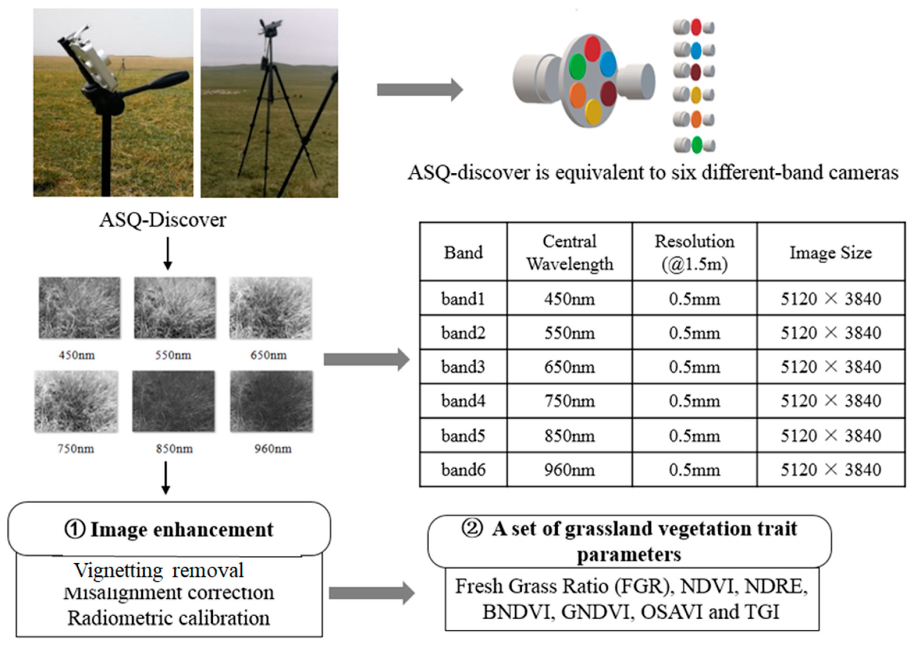
The ASQ-Discover is the hardware unit of the handheld grassland vegetation monitoring system, which mainly consists of a smartphone (Huawei Mate 9 Pro) and a filter wheel installed with 6 narrowband filters. The smartphone is set in monochrome image grabbing mode, and the 6-band filter device was miniaturized so that it could be attached to the smartphone. The ASQ-Discover utilizes a camera of the smartphone and the 6-band filter device for image acquisition. The working principle diagram of ASQ-Discover are shown in Figure 1. These six bands include three visible bands (450 nm, 550 nm, 650 nm), a red-edge band (750 nm), and two near-infrared bands (850 nm, 960 nm). The red-edge band is very effective for monitoring vegetation health. The 960 nm band corresponds to a strong absorption and can provide key information on the grass water content. The six filters are rotated by hand to acquire different band images under natural light conditions. The image size for every band is 5120 × 3840 pixels with 8-bit depth. The technical parameters of ASQ-Discover are also shown in Figure 1.
The data handling and analysis processes are divided into two parts (Figure 1). One part is image restoration through vignetting removal, radiometric calibration and misalignment correction; the other part is to establish a set of spectral traits of vegetation in order to describe grassland vegetation growth. The ASQ-Discover is equivalent to six different-band cameras, which capture a group of 6-band images. The group of 6-band images are restored by vignetting removal, misalignment correction and radiometric calibration, and then some spectral traits of vegetation are estimated and analyzed to understand grassland vegetation growth.
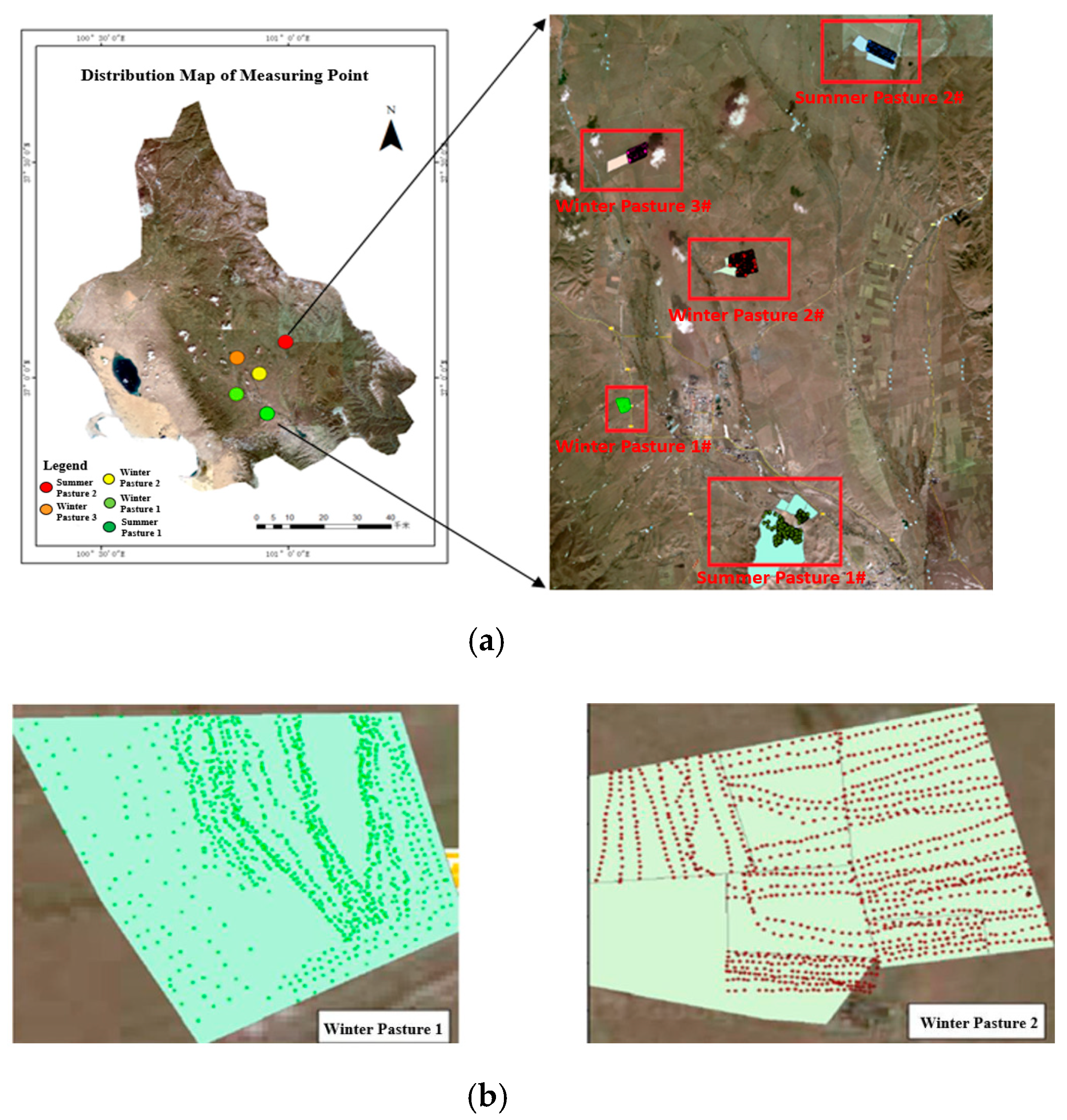
The field experiment was conducted in five pastures located in Haiyan County, Qinghai Province (east longitude: 100°85′ to 100°99′, North latitude: 36°91′ to 37°1′). The range of altitude is from 3090m to 3150m. In August 2017, May 2018, and July 2018, three field experiments were conducted on five pastures. The locations of the five pastures are shown in Figure 2a and the sampling coverage areas are summarized in Table 1. The experiments were conducted in summer pasture #2 and winter pasture #3 one time only in August 2017. The experiments were conducted in other pastures three times in August 2017, May 2018, and July 2018. The four ASQ-Discover systems were held separately to capture 6-band images of the pastures. The sampling distance between quadrats was about 20 m; for example, the quadrats in winter pasture #1 and winter pasture #2 are marked in Figure 2b, where the green and red points represent the quadrats. Each quadrat corresponds to a group of six-band images. To keep the same angle and height of capturing, the ASQ-Discover system was fixed on the tripod with about a 45 degree tilt considering the cover area of every image, and the ASQ-Discover system was about 1.5m above the ground. The ground resolution of the multispectral image is about 0.5 mm/pixel, which can capture the details of individual plants on the grassland. Image data were collected from 10 am to 2 pm under natural light condition, and each group of 6-band images needs about half a minute to be acquired and saved. The accumulated experiment area (all five pastures) is up to 6.2 km2 (in Table 1).
2.2. Image Processing
2.2.1. Vignetting Removal
The vignetting appeared in each band image because of sensor response, lens structure, and spectral variation of incident illumination. The vignetting is inevitable for close-range imaging. Some methods have been proposed for vignetting correction. Drew et al. used logarithmic analysis and a recursive method and a set of training data to find the optimal solution to the equation, which takes a long calculation time [17]. Khanna et al. proposed an outfield reflectivity correction method, but this method did not consider integration time and static noise [18]. Aasen et al. used the dark current to eliminate noise and choose a flat-field method to eliminate the influence of uneven illumination, but did not explicitly consider integral time [19]. They used a commonly used LUT method [20], which did not consider the integral time and dark current. These methods assume that the template or training data are acquired under the same illumination conditions and integral time. However, in the field, the illumination varies. To get a clear image, the ASQ-Discover was set in the automatic exposure mode, which can cause an uncertain integral time. The above methods are not applicable to the field data. Therefore, the vignetting correction method should consider integral time, dark current noise, and calculation time. The model of the vignetting correction is described as follows:
where and are the digital number (DN) value of the target image and reference image, respectively; and are the DN value of imaging in the dark current; and are the integral time of generating the target image and reference image; is the corrected DN of the target image. The reference images are some images of the write calibration panel captured using the ASQ-Discover, and the target images are some grassland images captured using the ASQ-Discover. The model of the vignetting correction reduces the effects of the integral time and dark current noise on vignetting.
2.2.2. Interband Misalignment Correction
There are small geometric misalignments between different band images because of the different thicknesses of filters and the vibration caused by the filter wheel, which needs to be corrected. Jhan et al. proposed a band geometric correction method for a 6-band imaging system [21], but the system consists of 6-band cameras, the position and attitude of the 6-band cameras are fixed, and they can be calibrated only one time. Brauers and Aach also proposed a geometric calibration method to eliminate the geometric errors between different band images from the multispectral imaging system with a filter wheel, which is feasible in theory [22]. However, geometric calibration in advance is not good for the multispectral imaging system with a filter wheel because of the uncertain vibration caused by rotating the filters every time. The geometric misalignments between different band images caused by rotating the filters are different every time; as result, they need to be re-calibrated every time.
In the early stages, our group studied geometric correction methods for multispectral imaging [23] and developed the corresponding batch processing software [24,25]. In [23,24,25], we described an airborne high resolution four-camera multispectral system that mainly consists of four identical monochrome cameras equipped with four interchangeable bandpass filters and proposed an automatic multispectral data composing method. The 4-band images were registered into a multispectral image through the homography registration model, the scale-invariant feature transform (SIFT), and random sample consensus (RANSAC). This algorithm without prior geometric calibration is suitable for the characteristics of the roller filter device. Due to the influence of central projection, the geometric errors increase gradually from the center to the edge. In order to batch these images quickly, four corner blocks and central blocks of the image are selected to be calculated. Then, we use the above method [23] to eliminate the small geometric misalignments between different bands.
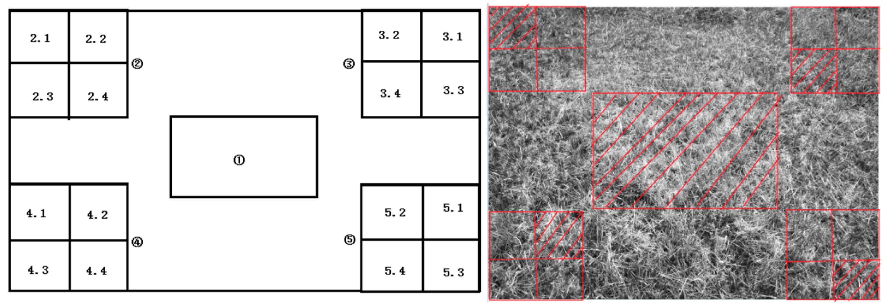
As shown in Figure 3, the image is divided into five blocks. Block 1 is a rectangle of size 1024 × 768, and blocks 2, 3, 4, 5 are four square areas of size 1600 × 1600 pixels at the corner of the image, which is divided into four equal squares (sub-blocks) and numbered in turn.
The sub-blocks with the most scale-invariant feature transform (SIFT) features are selected from the four corner blocks to match between different bands, such as 2.1, 3.4, 4.2, and 5.3. The selection of sub-blocks can not only improve the matching speed but can also ensure the uniform distribution of the image features.
2.2.3. Radiometric Calibration
After vignetting correction, the DNs of 6-band images are corrected, but they are not true representatives of the surface reflectance. Therefore, we should transform the corrected DNs of 6-band images into the physical radiance values for quantitative analysis; that is to say, radiometric calibration is a necessary step in this work. The physically based methods and empirical methods are the most commonly used calibration methods [26]. This study selected the empirical linear regression method (LRM) [27].
2.3. A Set of Spectral Traits of Vegetation
2.3.1. Selecting Vegetation Indices
A vegetation index (VI) is a spectral calculation that is done between two or more bands of the source data to enhance the contribution of vegetation properties. More than 150 vegetation indices (VI) [28] have been published in the scientific literature. According to the characteristics of ASQ-Discover, we selected NDVI (normalized difference vegetation index), NDRE (normalized difference red edge), BNDVI (blue normalized difference vegetation index), GNDVI (green normalized difference vegetation index), OSAVI (optimized soil-adjusted vegetation index) and TGI (triangular greenness index), and generate the high resolution NDVI, NDRE, BNDVI, GNDVI, OSAVI, and TGI images. The NDVI is an indicator to measure the photosynthetic activity of vegetation [29], and it is frequently employed as a proxy for plant greenness or vegetation growth [30]. The OSAVI is based on the NDVI but includes correction factors for the soil reflectance in the spectra, and it can reflect the result of cumulative water deficits [31,32]. The NDRE is an index sensitive to chlorophyll content in leaves against soil background effects [33]. TGI allows for the estimation of chlorophyll concentration in leaves and the canopy [34]. The BNDVI is also sensitive to chlorophyll content [35]. The GNDVI is an indicator of the photosynthetic activity of the vegetation cover, and it is most often used in assessing the moisture content and nitrogen concentration in plant leaves [36].
NDVI is built up from a combination of visual red light and near-infrared (NIR) light. The NDVI is linearly related to vegetation water potential [37,38]; 860 nm and 960 nm are both within the NIR region, but 960 nm corresponds to a strong absorption. In order to reflect the water content of vegetation, the 960 nm band is used to calculate the NDVI. Due to the OSAVI being based on the NDVI, the 960 nm band is also used to calculate the OSAVI. The VI formulas used in this study are shown in Table 2. These high resolution NDVI, NDRE, BNDVI, GNDVI, OSAVI, and TGI images are suitable for the ground-based analysis of green biomass, vegetative coverage, chlorophyll content, vegetation water content, and vegetation growth in grassland.
VIs derived from multi-spectral imaging (MSI) tools can be used to provide non-destructive phenotypes that could be used to better understand growth curves throughout the growing season [45,46]. This study used the ASQ-Discover to collect the multispectral images of each quadrat and generate vegetation index images in which each pixel value is a vegetation index (NDVI, NDRE, BNDVI, GNDVI, OSAVI, TGI). These high resolution NDVI, OSAVI, GNDVI, NDRE, BNDVI and TGI images are also suitable for the small-scale monitoring of natural grassland [35].
2.3.2. Estimating Fresh Grass Ratio
The period in which grass grows in Qinghai’s natural pastures is very short due to its particular environment and altitude. The fresh grass and hay always coexist over the whole growth period. The fresh grass ratio is critical information and reflects grassland productivity and the utilization rate of grassland resources.
The ASQ-Discover system can distinguish fresh grass and hay clearly because of the millimeter level resolution. There are some green vegetation indices such as ExG (Excess Green Index), ExR (Excess Red Index), VEG (Vegetative index), CIVE (Color Index of Vegetation Extraction), COM (Combined Indices) [47,48,49]. ExG is a popular index that is used in vegetation remote sensing because it is effective for extracting green plants. Another index is ExR, which can extract soil and plant residues. The ExG − ExR index is obtained by ExG minus ExR, and it has shown superior green vegetative separation accuracy under different environments (green house and field conditions) [47,48].
The formulas of ExG, ExR, and ExG − ExR indices are as follows:
where r, g, and b are normalized values for R, G, and B, and those indices are expressed as follows:
If the ExG − ExR value is negative, it represents soil or something nonliving, and if the value is positive it is green vegetation. Therefore, ExG − ExR is an efficient algorithm for detecting fresh grass (green vegetation) on grassland. Thus, the image pixels are classified as fresh grass, and the FGR is determined as the percentage of pixels classified as fresh grass per quadrat:
In this study, every quadrat corresponds to a multispectral image with six bands from the ASQ-Discover system.
3. Results
3.1. Vignetting Removal and Misalignment Correction
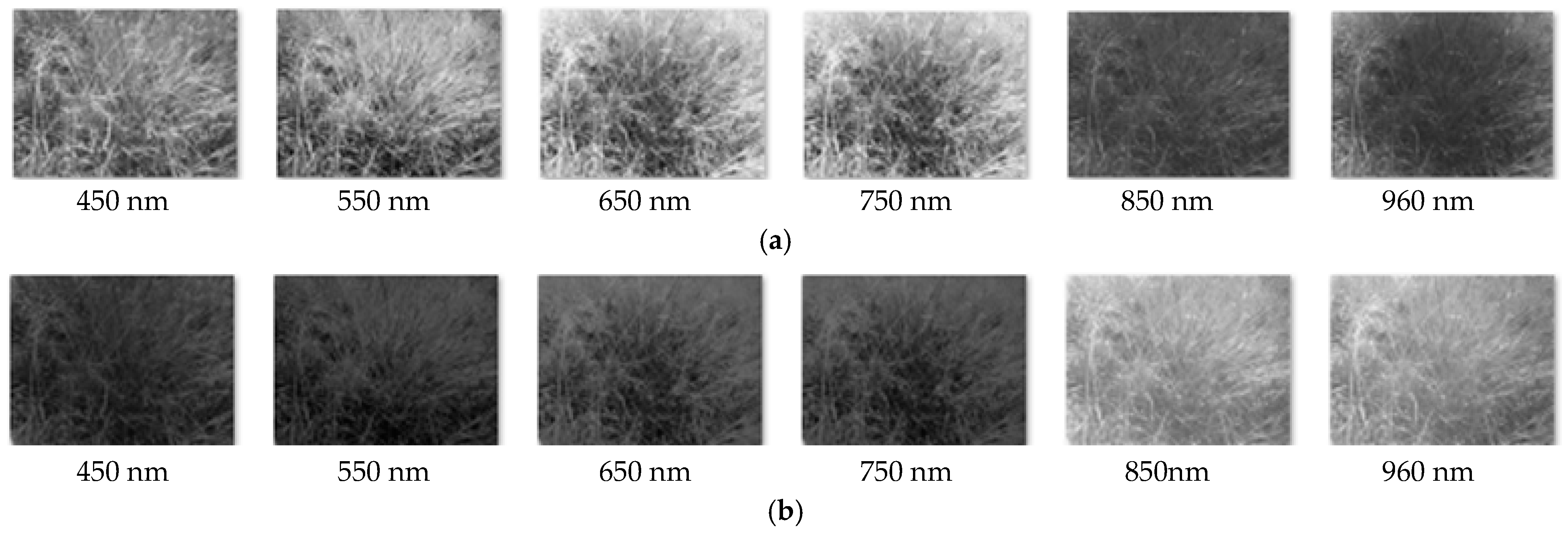
There are two main problems for the ASQ-Discover: vignetting and inter-band image misalignment. Influenced by the strong illumination on the Qinghai Plateau and the close range, vignetting distinctly appeared in each band image we captured (in Figure 4a).
Figure 4b is the results of vignetting correction using the method proposed in this paper. The vignetting phenomenon is related to the structure parameters of the camera, the lens, the dynamic variation of illumination, and the reflected spectrum. We found the vignetting degrees in different wavelengths were different, especially in the near-infrared band (Figure 4a).
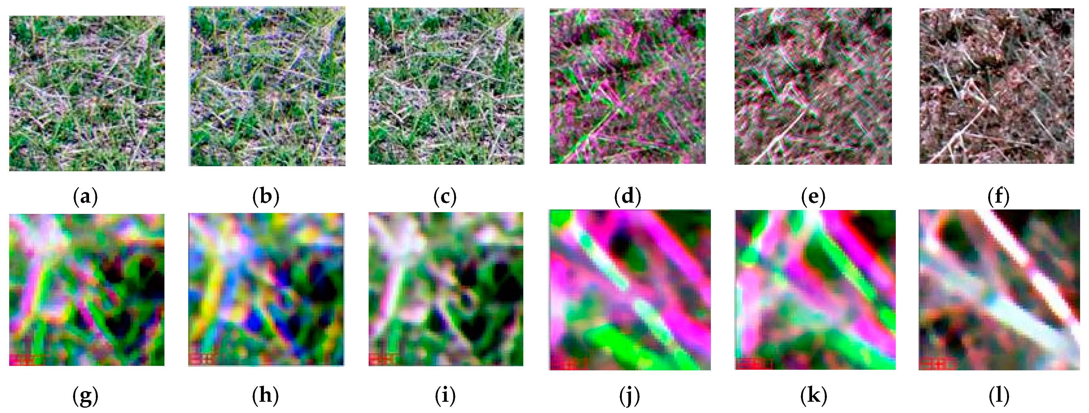
Due to the different thicknesses of the filters and the unavoidable mechanical disturbance during the measurement process, including filter wheel rotation, lens auto-focus adjustment, and slight sample movement, there are small misalignments between different band images (Figure 5). Figure 5 shows the geometric matching results of different band images obtained by different methods. Table 3 shows the average errors of matching using different methods when the reference image is the 450 nm band, which clearly indicates that the results when using our method are better.
However, the ASQ-Discover cannot grab 6-band images at the same time due to rotating the filter wheel. While capturing the grass images, these grasses can be moved by the wind so that there are still some very small misalignments caused by the wind between different band images after geometric correction.
3.2. Radiometric Calibration
Radiometric calibration was executed for the quantification of image DN values to surface reflectance values. Four calibration cloths were used to collect the field spectra, and the reflectance of them are from 5%, 20%, 40%, and 60%. This study has captured 20 groups of 6-band images of each calibration cloth from different directions. The DNs of images were corrected by the method mentioned in Section 2.2.1. Moreover, this study calculated the mean corrected DNs for each band of the Region of Interest (ROIs) extracted from the calibration cloth images. The spectral measurement of each calibration cloth was achieved using an ASD spectroradiometer from different directions. The mean spectral measurement of each calibration cloth was also calculated. The LRM method was used to obtain the calibration equation of each band in Table 4. Our results showed a statistically significant relationship in all spectral bands. Coefficient of determination R2 = 0.92–0.94 was achieved in all bands, indicating that the relationship between the image DN and reflectance is linear.
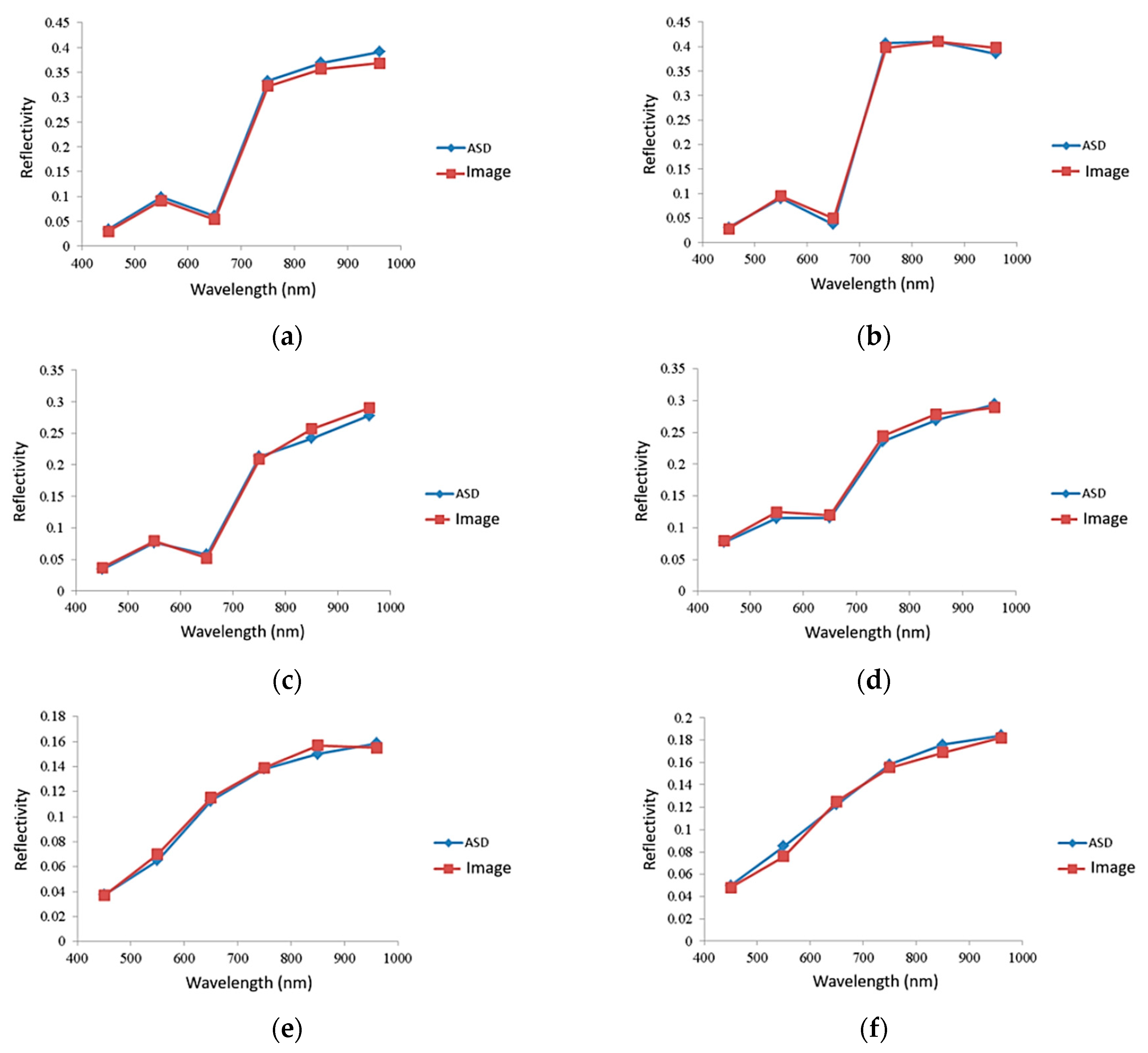
In the study area, we chose fresh grasses, hays, and soils as validation targets. The calibrated reflectance values from images were compared with the field-measured reflectance values using ASD, and the compared results are illustrated in Figure 6. The calibrated reflectance values are very close to the field-measured reflectance values. The Mean Absolute Percent Error (MAPE) value of each band between the calibrated reflectance values and the field-measured reflectance values was calculated via Equation (7), using 30 samples of each kind of validation target in Table 5. The highest MPAE of 17.62% was observed in an 850 nm band and the lowest MPAE of 2.19% was observed in a 750 nm band.
where is the calibrated reflectance value and is the field-measured reflectance value.
3.3. Visualization of the Selected Vegetation Indices at Quadrat Level
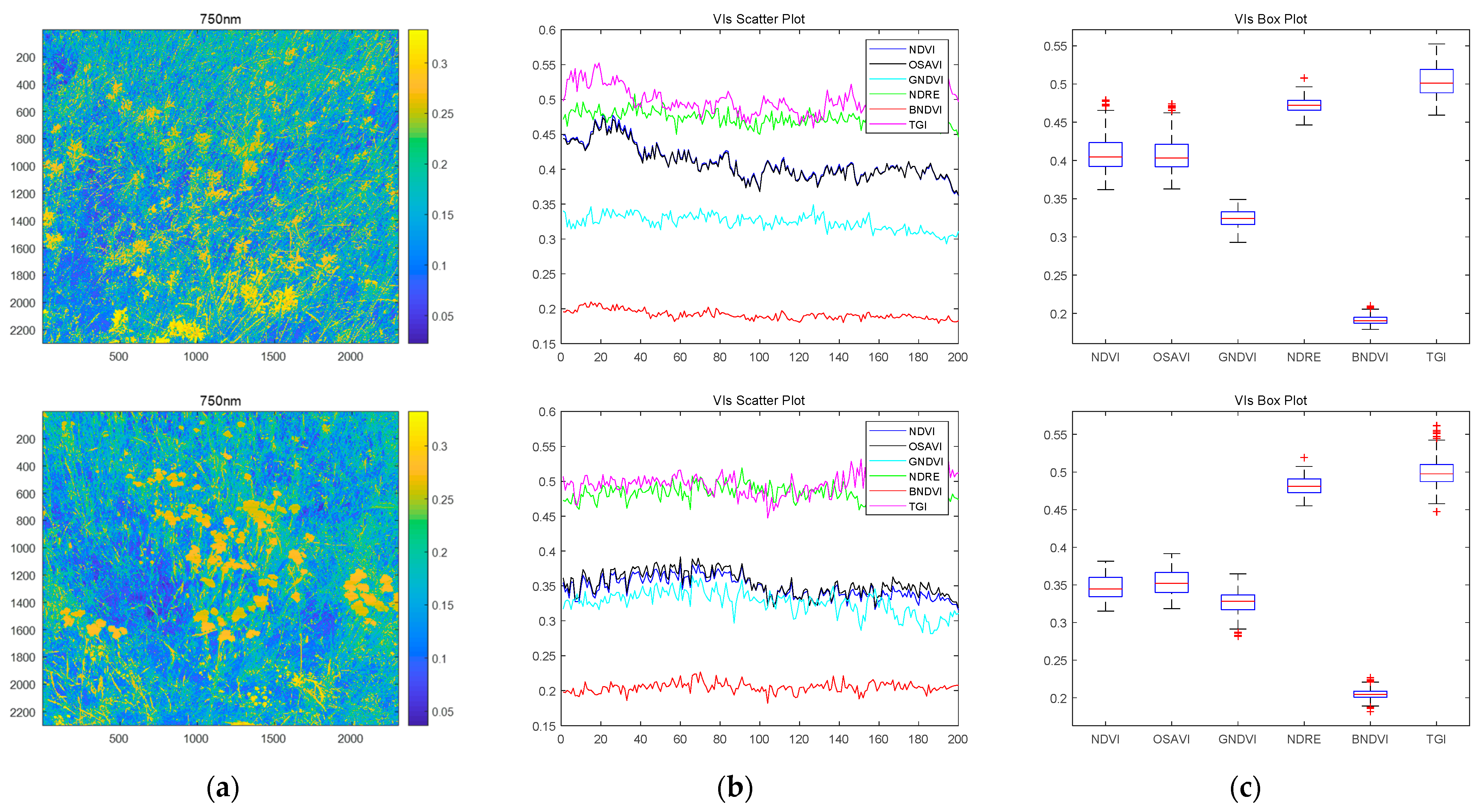
Considering the speed of the batch processing, we selected the center region 2300 × 2300 pixels from the multispectral images to generate the NDVI, OSAVI, GNDVI, NDRE, BNDVI, and TGI images. Then, we randomly selected 200 columns in the VI images to calculate the means of the NDVI, OSAVI, GNDVI, NDRE, BNDVI, and TGI for each column and used them to make scatter plots. At the same time, we utilized box plots to illustrate the distribution of the six vegetation indices.
Figure 7 corresponds to two multispectral images randomly selected, which were captured in July 2018. The scatter plots and box plots of the six vegetation indices are shown in Figure 7b, and the corresponding 750 nm images are shown in Figure 7a. The values of the six vegetation indices are visualized clearly in the VI scatter plots and VI box plots.
3.4. An Analysis of the Selected Vegetation Indices at Pasture Level
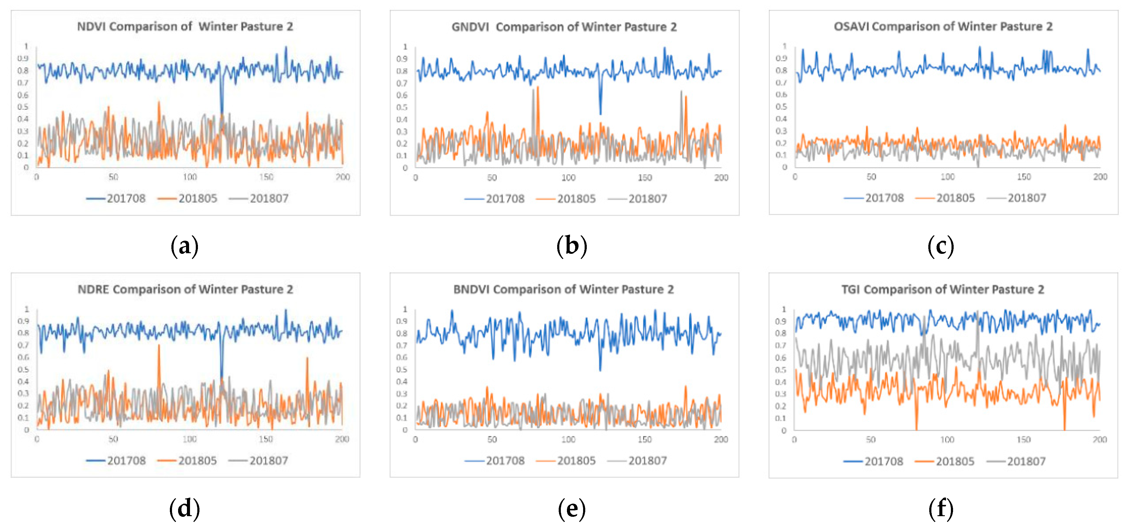
In order to compare the six vegetation indices’ values (NDVI, OSAVI, GNDVI, NDRE, BNDVI, and TGI) for the same pasture at different times, 200 quadrats were randomly, selected in August 2017, May 2018, and July 2018 of winter pasture #2. The means of the six vegetation indices were computed and are shown in Figure 8. The VI values were normalized in order to compare them. The natural growth cycle of grassland on the Qinghai plateau was divided into four stages, such as the re-greening phase (April–June), the grass-bearing phase (July–September), the yellowing phase (October–December), and the dry grass phase (January–March). The VI values in August 2017 are higher than those in May 2018 and July 2018, and the VI values in July 2018 are closer to those in May 2018. In other words, the grassland vegetation exhibited better growing trends in August 2017.
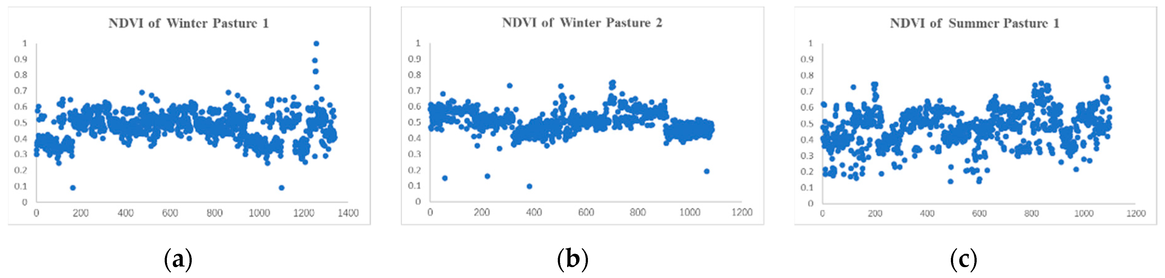
Figure 9 shows the distribution of the NDVI values in July 2018 between the winter pastures and the summer pastures. It was found that the distribution of the NDVI values in the winter pastures were more concentrated in a smaller range, while the distribution of the NDVI values in summer pastures are scattered. In July, the herds are driven to summer pastures, the grass of summer pastures is grazed, and their NDVI values varied greatly. On the other hand, the NDVI values in the winter pasture are much more stable because this grass is not grazed.
3.5. Fresh Grass Ratio
Meyer and other researchers have shown that the ExG − ExR calculated from the data of a color digital camera is very effective for separating single plants from soil with a fixed 0 threshold [47]. However, Qinghai grassland is a complex green vegetation type, which means it is necessary to find the optimal threshold to extract the fresh grass regions from the multispectral images.
Taking winter pasture #1 as an example, Figure 10 and Figure 11 are a group of multispectral images from ASQ-Discover, which were captured on winter pasture #1 in May 2018. There were fresh grass, hay grass, and soil in these multispectral images.
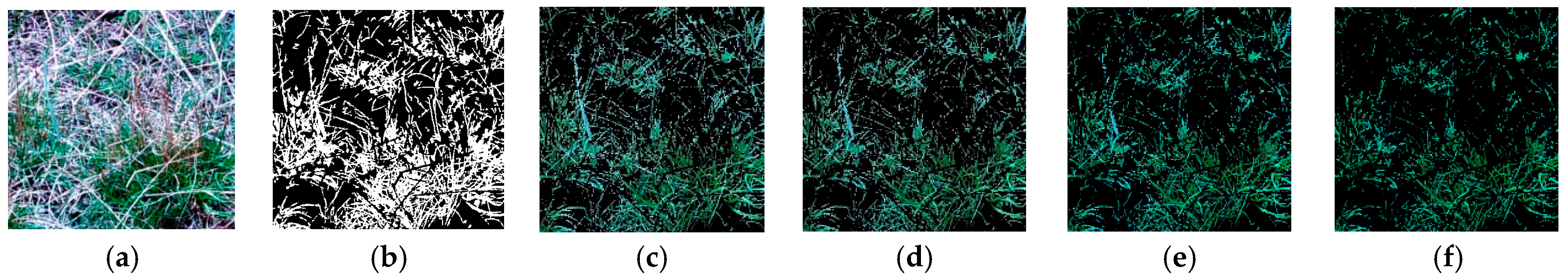
To find an appropriate threshold, this study examined the accuracy rates of the segmentation () at different thresholds for the test image. The hand-generated template image using photoshop was used as the truth value [47] (Figure 10b). All green plant pixels were set to white, and the background pixels were set to black to form a binary reference.
The ExG − ExR method was applied to classify all the pixels of the test image into two classes as fresh grass or background. Figure 10 shows the segmentation results and the accuracy rates of the segmentation with different threshold. It was not hard to find that the accuracy rate in 0 threshold was 0.9363, which is greater than that in other thresholds. Therefore, this study chose 0 as the classification threshold of fresh grass in the research area.
The accuracy rate of the segmentation can be expressed as [47]:
where is a truth set of manually separated fresh grass pixels (T(i,j) = 255) or background (T(i,j) = 0), corresponding to the hand-generated template image; is a set of fresh grass pixels () or others () based on the classification results, i and j are the row and column indices for the image, respectively, and M and N are the image row and column size, respectively.
According to Equation (8), vegetation separation accuracy is based on a logical or “∩” and a logical and “∪”, compared on a pixel by pixel basis of target image I to the template image T. A of 1.0 represents a perfect index extraction of all selected class pixels, while a near 0.0 represents no class extraction in set T [47].
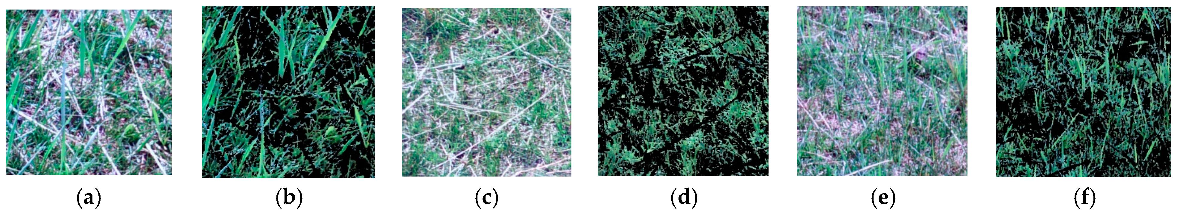
This study used this threshold to extract the fresh grass pixels from the multispectral images of all quadrats. The part results are shown in Figure 11.
Additionally, then we used the classification threshold to extract the fresh grass pixels from the multispectral images of all quadrats. The results, in part, are shown in Figure 10. Thus, the fresh grass ratio (FGR) of each quadrat was calculated using the FGR formula.
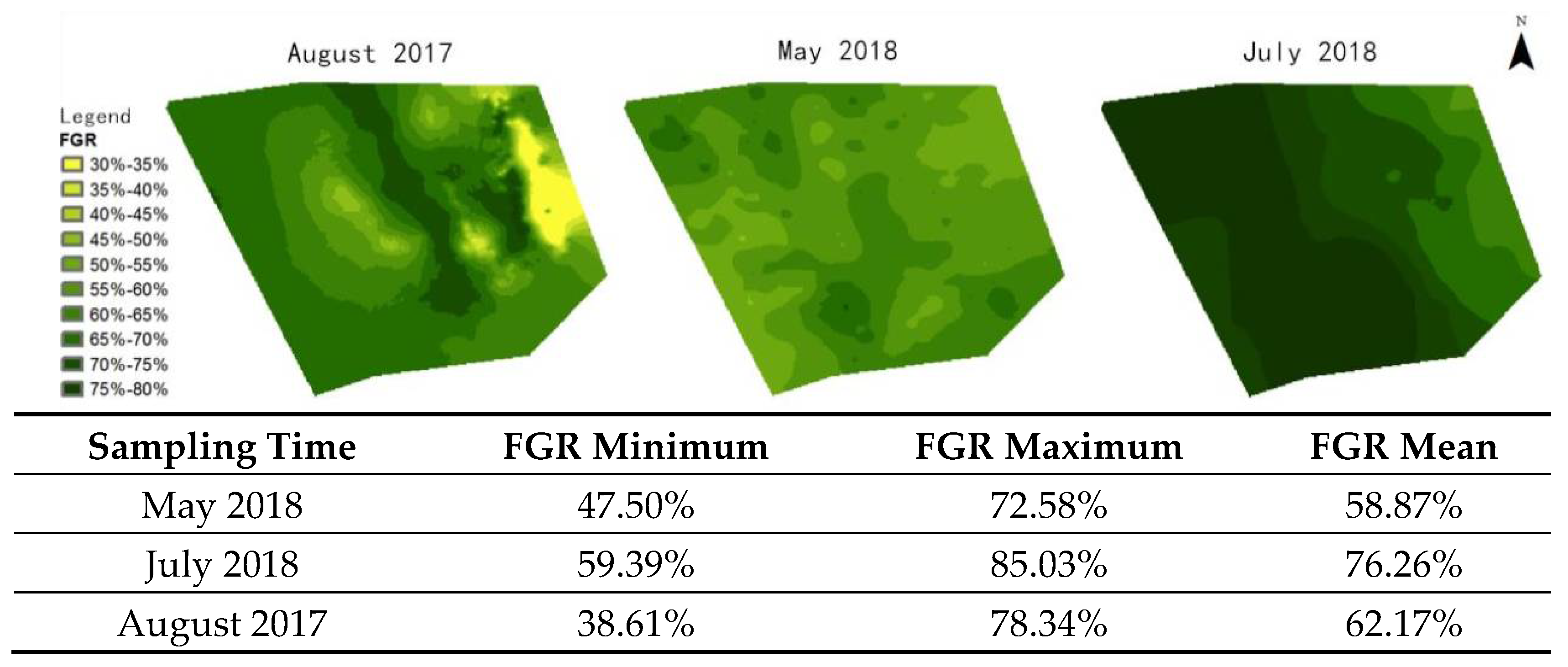
In this study, the research pastures are flat, and the sampling distance between quadrats is about 20 m. The classical Bayesian Kriging interpolation algorithm was used to produce an FGR map of the whole pasture (in Figure 12), and the statistics were given in Figure 12. The FGR values in July 2018 are higher than those in May 2018 and August 2017, while the FGR values in August 2017 are closer to those in July 2018 than those in May 2018.
4. Discussion
The goal of this paper is to develop a close-range handheld grassland vegetation monitoring system based on multispectral imaging. Some equipment of multispectral imaging or hyperspectral imaging is expensive, and it has to be operated by experts, which are serious limiting factors in its applications [50]. In this paper, the grassland vegetation monitoring system we propose reconciles the requirements for simple, cost-effective accurate, in-field optical measurements. However, the close-range multispectral images are different from satellite images and UAV images. The close-range multispectral imaging is a challenging task and suffers from technical complexities related to external factors (e.g., illumination effects) and vegetation-related factors (e.g., complex vegetation geometry) [51]. Therefore, the limitations and advantages of the system are discussed in this section.
(1) Vignetting is a challenge for close-range imaging. In the field, the illumination changes dynamically. In order to get a clear image, the ASQ-Discover is set in automatic exposure mode that can lead to an uncertain integration time. Because the sensor pixel response is inconsistent, there is static noise named dark current noise for the imaging system. Many vignetting correction methods do not consider the integration time and dark current noise. We used a simple correction method considering both integration time and dark current noise, which is more suitable to process the images captured in the field.
(2) We proposed a block-based multispectral image registration method to eliminate the inter-band misalignment. Compared with the traditional local and global optimization methods applied to whole images, the sub-blocks can not only improve the matching speed but also ensure the uniform distribution of the SIFT features and avoids the risk of trapping into a local minimum.
(3) We employed the empirical linear regression method (LRM) to perform radiometric calibration of ASQ-Discover images. In the study area, we chose fresh grasses, hays, and soils as validation targets and compared the calibrated reflectance values from images with the canopy-measured reflectance values using an ASD spectroradiometer. Due to the very high resolution of the ASQ-Discover images, some factors, such as grassland heterogeneity, different scale, and varying illumination, caused relatively high radiometric calibration error of the 850 nm band in the case of grassland reflectance [51,52].
(4) We established a set of spectral traits of vegetation and estimated them using some simple methods. The spectral traits of vegetation include FGR and some vegetation indices, which represent mathematical combinations of surface reflectance at two or more wavelengths such as NDVI, GNDVI, BNDVI, NDRE, OSAVI and TGI. The FGR is a key parameter of grass growth status. We estimated the FGR using the ExG − ExR index, which is a simple method to separate fresh grasses from their backgrounds. NDVI, NDRE, BNDVI, GNDVI, OSAVI, and TGI can reflect chlorophyll, nutrient, and vegetation growth.
(5) Compared to spaceborne, airborne, or unmanned aerial vehicle (UAV) platforms, the handheld grassland vegetation growth monitoring system proposed in this study can be mastered and operated by operators with minimal or no training. In addition, this study was carried out on the pastures of the Qinghai Plateau, the plateau environmental conditions have special power requirements for airships and UAVs at high altitudes, while the handheld grassland vegetation growth monitoring system is more suitable for the grass growth status survey of Qinghai plateau.
(6) Most of the relatively low-cost commercial sensors available on the market, such as MicaSense Multispectral Sensors [53] and Tetracam’s Micro-Miniature Multiple Camera Array System [54], use several independent cameras with different filters to capture different band images. In addition, most relatively low-cost commercial sensors are developed for UAV remote sensing and are not appropriate for deployment with handheld devices. In this paper, the ASQ-Discover attached a 6-band filter device to a smartphone for different band image acquisition. Except for the 6-band filter device, it entirely utilizes the high-resolution camera, operating system, GPS, and wireless module of the smartphone. In other words, the ASQ-Discover can be regarded as a multiband mobile phone, which also tends to cost less and to require cheaper hardware than the more-common commercial sensors on the market. However, there are many significant improvements that still need to be made before it becomes a mature application. We found that there is still a little vignetting kept in the near-infrared band image after vignetting correction under strong natural light. Due to the ASQ-Discover being unable to grab 6-band images at the same time while capturing the grass images these grasses can be moved in the wind that leads to small misalignments caused by the wind, which can still exit after geometric correction.
Although high resolution images can capture the details of individual plants on the grassland, high resolution can cause some errors. In the future, we will look into some new methods of processing the high-resolution images. The manual rotation of the filter device is inconvenient, and in the future we will develop an automatic filter wheel device instead of using a manual one.
5. Conclusions
This study developed a handheld grassland vegetation growth monitoring system; discussed the image processing methods for the close-range imaging, including vignetting correction, radiometric calibration, and misalignment correction; and established a set of spectral traits of vegetation to describe grassland vegetation growth. The results show that the system proposed in this paper can be used to monitor grassland vegetation growth. This study also confirmed the potential of a handheld grassland monitoring system that can be used for accurate grassland vegetation trait measurements.
Author Contributions
Conceptualization, A.Z. and S.H.; methodology, A.Z. and S.H.; hardware, S.H.; software, A.Z., X.Z. and T.Z.; validation, A.Z., X.Z. and T.Z.; formal analysis, A.Z.; investigation, S.H.; resources, S.H.; data curation, A.Z.; writing—original draft preparation, S.H. and A.Z.; writing—review and editing, X.Z., M.L., H.T. and Y.H.; supervision, S.H.; project administration, A.Z.; funding acquisition, A.Z. All authors have read and agreed to the published version of the manuscript.
Funding
This research was funded by the National Natural Science Foundation of China, Grant Number 42071303 and the Special Foundation for Science and Technology Basic Resource Investigation Program of China, Grant Number 2019FY101304.
Acknowledgments
The authors would like to thank the anonymous reviewers and the editor for their constructive comments and suggestions for this study.
Conflicts of Interest
The authors declare no conflict of interest. The funders had no role in the design of the study; in the collection, analyses, or interpretation of data; in the writing of the manuscript; or in the decision to publish the results.
References
- Capolupo, A.; Kooistra, L.; Berendonk, C.; Boccia, L.; Suomalainen, J. Estimating plant traits of grasslands from UAV-acquired hyperspectral images: A comparison of statistical approaches. ISPRS Int. J. Geo Inf. 2015, 4, 2792–2820. [Google Scholar] [CrossRef]
- Homolová, M.E.; Schaepman, P.; Lamarque, J.G.; de Bello Clevers, F.; Thuiller, W.; Lavorel, S. Comparison of remote sensing and plant trait-based modelling to predict ecosystem services in subalpine grasslands. Ecosphere 2014, 5, 1–29. [Google Scholar] [CrossRef]
- Pullanagari, R.R.; Kereszturi, G.; Yule, I. Integrating airborne hyperspectral, topographic, and soil data for estimating pasture quality using recursive feature elimination with random forest regression. Remote. Sens. 2018, 10, 1117. [Google Scholar] [CrossRef] [Green Version]
- Zhang, A.; Guo, C.; Yan, W. Improving remote sensing estimation accuracy of pasture crude protein content by interval analysis. Trans. Chin. Soc. Agric. Eng. (Trans. CSAE) 2018, 34, 149–156. [Google Scholar]
- Zhang, A.; Yan, W.; Guo, C. Inversion model of pasture crude protein content based on hyperspectral image. Trans. Chin. Soc. Agric. Eng. (Trans. CSAE) 2018, 34, 188–194. [Google Scholar]
- Thenkabail, P.S.; Lyon, J.G. Hyperspectral Remote Sensing of Vegetation; CRC Press: Boca Raton, FL, USA, 2016. [Google Scholar]
- Lopatin, J.; Fassnacht, F.E.; Kattenborn, T.; Schmidtlein, S. Mapping plant species in mixed grassland communities using close range imaging spectroscopy. Remote. Sens. Environ. 2017, 201, 12–23. [Google Scholar] [CrossRef]
- Mccann, C.; Repasky, K.S.; Lawrence, R.; Powell, S. Multi-temporal mesoscale hyperspectral data of mixed agricultural and grassland regions for anomaly detection. Isprs. J. Photogramm. Remote. Sens. 2017, 131, 121–133. [Google Scholar] [CrossRef]
- Neumann, C.; Förster, M.; Kleinschmit, B.; Itzerott, S. Utilizing a PLSR-Based Band-Selection Procedure for Spectral Feature Characterization of Floristic Gradients. IEEE J. Sel. Top. Appl. Earth Obs. Remote. Sens. 2016, 9, 1–15. [Google Scholar] [CrossRef]
- Gutiérrez, S.; Wendel, A.; Underwood, J. Ground based hyperspectral imaging for extensive mango yield estimation. Comput. Electron. Agric. 2019, 157, 126–135. [Google Scholar] [CrossRef]
- Chebrolu, N.; Lottes, P.; Schaefer, A.; Winterhalter, W.; Burgard, W.; Stachniss, C. Agricultural robot dataset for plant classification, localization and mapping on sugar beet fields. Int. J. Robot. Res. 2017, 36, 1045–1052. [Google Scholar] [CrossRef] [Green Version]
- Rebetzke, G.J.; Jimenezberni, J.A.; Bovill, W.D.; Deery, D.M.; James, R.A. High-throughput phenotyping technologies allow accurate selection of stay-green. J. Exp. Bot. 2016, 67, 4919–4924. [Google Scholar] [CrossRef] [PubMed] [Green Version]
- Fern, R.R.; Foxley, E.A.; Bruno, A.; Morrison, M.L. Suitability of NDVI and OSAVI as estimators of green biomass and coverage in a semi-arid rangeland. Ecol. Indic. 2018, 94, 16–21. [Google Scholar] [CrossRef]
- Hill, M.J. Vegetation index suites as indicators of vegetation state in grassland and savanna: An analysis with simulated SENTINEL 2 data for a North American transect. Remote. Sens. Environ. 2013, 137, 94–111. [Google Scholar] [CrossRef]
- Behmann, J.; Acebron, K.; Emin, D.; Bennertz, S.; Matsubara, S.; Thomas, S.; Bohnenkmp, D.; Kuska, T.M.; Mahlein, A.K.; Rascher, U.; et al. Specim IQ: Evaluation of a New, Miniaturized Handheld Hyperspectral Camera and Its Application for Plant Phenotyping and Disease Detection. Sensors 2018, 18, 441. [Google Scholar] [CrossRef] [Green Version]
- Ma, Z.; Mao, Y.; Liang, G.; Liu, C. Smartphone-Based Visual Measurement and Portable Instrumentation for Crop Seed Phenotyping. IFAC Pap. 2016, 49, 259–264. [Google Scholar]
- Drew, M.S.; Finlayson, G.D. Analytic solution for separating spectra into illumination and surface reflectance components. J. Opt. Soc. Am. A 2017, 2, 294–303. [Google Scholar] [CrossRef] [Green Version]
- Khanna, R.; Sa, I.; Nieto, J.; Siegwart, R. On field radiometric calibration for multispectral cameras. In Proceedings of the 2017 IEEE International Conference on Robotics and Automation (ICRA), Singapore, 29 May–3 June 2017; pp. 6503–6509. [Google Scholar] [CrossRef]
- Aasen, H.; Burkart, A.; Bolten, A.; Bareth, G. Generating 3D hyperspectral information with lightweight UAV snapshot cameras for vegetation monitoring: From camera calibration to quality assurance. ISPRS J. Photogramm. Remote. Sens. 2017, 108, 245–259. [Google Scholar] [CrossRef]
- Ahmed, E.; Rose, J. The effect of LUT and cluster size on deep-submicron FPGA performance and density. IEEE Trans. Very Large Scale Integr. (VLSI) Syst. 2000, 12, 288–298. [Google Scholar] [CrossRef] [Green Version]
- Jhana, J.; Raua, J.; Huang, C. Band-to-band registration and ortho-rectification of multilens/multispectral imagery: A case study of MiniMCA-12 acquired by a fixed-wing UAS. ISPRS J. Photogramm. Remote. Sens. 2016, 114, 66–77. [Google Scholar] [CrossRef]
- Brauers, J.; Aach, T. Geometric Calibration of Lens and Filter Distortions for Multispectral Filter-Wheel Cameras. IEEE Trans. Image Process. 2011, 20, 496–505. [Google Scholar] [CrossRef]
- Li, H.; Zhang, A.; Hu, S. A multispectral image creating method for a new airborne four-camera system with different bandpass filters. Sensors 2015, 15, 17453–17469. [Google Scholar] [CrossRef] [PubMed] [Green Version]
- Zhang, A.; Li, H. A Lateral Strip Fast Splicing Method Without Shadows for Aerial Video Images. Chinese Patent No. 201511025377.3, 2 November 2018. [Google Scholar]
- Zhang, A.; Li, H. Multispectral Registration and Combination Software. Chinese Software Copyright No. 2015SR00768, 14 January 2015. [Google Scholar]
- Guo, Y.; Senthilnath, J.; Wu, W.; Zhang, X.; Zeng, Z.; Huang, H. Radiometric Calibration for Multispectral Camera of Different Imaging Conditions Mounted on a UAV Platform. Sustainability 2019, 11, 978. [Google Scholar] [CrossRef] [Green Version]
- W M Baugh, D.P.G. Empirical proof of the empirical line. Int. J. Remote. Sens. 2008, 29, 665–672. [Google Scholar] [CrossRef]
- Available online: https://en.wikipedia.org/wiki/Vegetation_Index (accessed on 16 August 2021).
- Zhang, H.; Ma, J.; Chen, C.; Tian, X. NDVI-Net: A fusion network for generating high-resolution normalized difference vegetation index in remote sensing. ISPRS J. Photogramm. Remote. Sens. 2020, 168, 182–196. [Google Scholar] [CrossRef]
- Pei, F.; Wu, C.; Liu, X.; Li, X.; Yang, K.; Zhou, Y.; Wang, K.; Xu, L.; Xia, G. Monitoring the vegetation activity in China using vegetation health indices. Agric. For. Meteorol. 2018, 248, 215–227. [Google Scholar] [CrossRef]
- Baluja, J.; Diago, M.P.; Balda, P.; Zorer, R.; Meggio, F.; Morales, F.; Tardguila, J. Assessment of vineyard water status variability by thermal and multispectral imagery using an unmanned aerial vehicle (UAV). Irrig. Sci. 2012, 30, 511–522. [Google Scholar] [CrossRef]
- Ihuoma, S.O.; Madramootoo, C.A. Crop reflectance indices for mapping water stress in greenhouse grown bell pepper, Agricultural Water Management. Agric. Water Manag. 2019, 219, 49–58. [Google Scholar] [CrossRef]
- Available online: https://eos.com/industries/agriculture/ndre (accessed on 16 August 2021).
- Fernandez-Gallego, J.A.; Kefauver, S.C.; Vatter, T.; Gutiérrezd, N.A.; NietoTaladrize, M.T.; Araus, J.L. Low-cost assessment of grain yield in durum wheat using RGB images. Eur. J. Agron. 2019, 105, 146–156. [Google Scholar] [CrossRef]
- Kleed, A.; Gypser, S.; Herppich, W.B.; Bader, G.; Veste, M. Identification of spatial pattern of photosynthesis hotspots in moss- and lichen-dominated biological soil crusts by combining chlorophyll fluorescence imaging and multispectral BNDVI images. Pedobiologia 2018, 68, 1–11. [Google Scholar] [CrossRef] [Green Version]
- Available online: https://www.soft.farm/en/blog/vegetation-indices-ndvi-evi-gndvi-cvi-true-color-140 (accessed on 16 August 2021).
- Aguilar, C.; Zinnert, J.C.; Polo, M.J.; Young, D.R. NDVI as an indicator for changes in water availability to woody vegetation. Ecol. Indic. 2012, 23, 290–300. [Google Scholar] [CrossRef]
- Chen, H.; Wang, P.; Li, J.; Zhang, J.; Zhong, L. Canopy Spectral Reflectance Feature and Leaf Water Potential of Sugarcane Inversion. Phys. Procedia 2012, 25, 595–600. [Google Scholar] [CrossRef] [Green Version]
- Tucker, C.J. Cover Maximum normalized difference vegetation index images for sub-Saharan Africa for 1983–1985. Int. J. Remote. Sens. 1986, 7, 1383–1384. [Google Scholar] [CrossRef]
- Steven, M.D. The sensitivity of the OSAVI vegetation index to observational parameters. Remote. Sens. Environ. 1998, 63, 49–60. [Google Scholar] [CrossRef]
- Rondeaux, G.; Steven, M.; Baret, F. Optimization of Soil-Adjusted Vegetation Indices. Remote. Sens. Environ. 1996, 55, 95–107. [Google Scholar] [CrossRef]
- Shanahan, J.F.; Schepers, J.S.; Francis, D.D.; Varvel, G.E.; Wilhelm, W.W.; Tringe, J.M.; Schlemmer, M.R.; Major, D.J. Use of Remote-Sensing Imagery to Estimate Corn Grain Yield. Agron. J. 2001, 93, 583. [Google Scholar] [CrossRef] [Green Version]
- Li, F.; Miao, Y.; Feng, G.; Yuan, F.; Yue, S.; Gao, X.; Liu, Y.; Liu, B.; Ustin, S.L.; Chen, X.; et al. Improving estimation of summer maize nitrogen status with red edge-based spectral vegetation indices. Field Crop. Res. 2014, 157, 111–123. [Google Scholar] [CrossRef]
- Hunt, E.R., Jr.; Doraiswamy, P.C.; McMurtrey, J.E.; Daughtry, C.S.T.; Perry, E.M.; Akhmedov, B. A visible band index for remote sensing leaf chlorophyll content at the canopy scale. Int. J. Appl. Earth Obs. Geoinf. 2013, 21, 103–112. [Google Scholar] [CrossRef] [Green Version]
- Wu, G.; Miller, N.D.; Leon, N.; Kaeppler, S.M.; Spalding, E.P. Predicting Zea mays Flowering Time, Yield, and Kernel Dimensions by Analyzing Aerial Images. Front. Plant Sci. 2019, 10, 12–51. [Google Scholar] [CrossRef] [Green Version]
- Anche, M.T.; Kaczma, N.S.; Morales, N.; Clohessy, J.W.; Ilut, D.C.; Gore, M.A.; Robbins, K.R. Temporal covariance structure of multi spectral phenotypes and their predictive ability for end of season traits in maize. Theor. Appl. Genet. 2020, 133, 2853–2868. [Google Scholar] [CrossRef] [PubMed]
- Meyer, G.E.; Neto, J.C. Verification of color vegetation indices for automated crop imaging applications. Comput. Electron. Agric. 2008, 63, 282–293. [Google Scholar] [CrossRef]
- Hamuda, E.; Glavin, M.; Jones, E. A survey of image processing techniques for plant extraction and segmentation in the field. Comput. Electron. Agric. 2016, 125, 184–199. [Google Scholar] [CrossRef]
- Zhang, D.; Mansaray, L.R.; Jin, H.; Han, S.; Kuang, Z.; Huang, J. A universal estimation model of fractional vegetation cover for different crops based on time series digital photographs. Comput. Electron. Agric. 2018, 151, 93–103. [Google Scholar] [CrossRef]
- Kitić, G.; Tagarakis, A.; Cselyuszka, N.; Panić, M.; Birgermajer, S.; Sakulski, D.; Matović, J. A new low-cost portable multispectral optical device for precise plant status assessment. Comput. Electron. Agric. 2019, 162, 300–308. [Google Scholar] [CrossRef]
- Mishra, P.; Asaari, M.S.M.; Herrero-Langreo, A.; Lohumi, S.; Diezma, B.; Scheunders, P. Close range hyperspectral imaging of plants: A review. Biosyst. Eng. 2017, 164, 49–67. [Google Scholar] [CrossRef]
- Iqbal, F.; Lucieer, A.; Barry, K. Simplified radiometric calibration for UASmounted multispectral sensor. Eur. J. Remote Sens. 2018, 51, 301–313. [Google Scholar] [CrossRef]
- MicaSense Multispectral Sensors. Available online: https://micasense.com (accessed on 16 August 2021).
- Tetracam Micro-MCA Multispectral Camera Array. Available online: https://tetracam.com/Products-Micro_MCA.htm (accessed on 16 August 2021).
Figure 1.
The working principle, technical parameters, and workflow of the grassland vegetation state monitoring system.
Figure 1.
The working principle, technical parameters, and workflow of the grassland vegetation state monitoring system.

Figure 2.
The location of pastures and distribution of quadrats: (a) the location of the five pastures (summer pasture #1, summer pasture #2, winter pasture #1, winter pasture #2, winter pasture #3); (b) distribution of quadrats on the pastures, the green and red points represent the quadrats).
Figure 2.
The location of pastures and distribution of quadrats: (a) the location of the five pastures (summer pasture #1, summer pasture #2, winter pasture #1, winter pasture #2, winter pasture #3); (b) distribution of quadrats on the pastures, the green and red points represent the quadrats).

Figure 3.
Image block partition schematic map.

Figure 4.
The results of vignetting correction. (a) Uncorrected 6-band images. (b) Corrected 6-band images.
Figure 4.
The results of vignetting correction. (a) Uncorrected 6-band images. (b) Corrected 6-band images.

Figure 5.
Misalignment correction results using different methods. (a–c) The images consist of 450 nm, 550 nm, and 650 nm bands. (d–f) The images consist of 750 nm, 850 nm, and 960 nm bands. (a,d) Unmatched image. (b,e) The whole image matching. (c,f) Only image block matching. (g–i) The enlarged results of (a–c). (j–l) The enlarged result of (d–f).

Figure 6.
The compared results between the calibrated reflectance values and the field-measured reflectance values. Two samples of each kind of validation targets were listed as: (a,b) are fresh grass; (c,d) are hay; (e,f) are soil.
Figure 6.
The compared results between the calibrated reflectance values and the field-measured reflectance values. Two samples of each kind of validation targets were listed as: (a,b) are fresh grass; (c,d) are hay; (e,f) are soil.

Figure 7.
Visualization of six selected vegetation indices. (a) The 750 nm images. (b) The scatter plots of the six vegetation indices. (c) The box plots of the six vegetation indices.
Figure 7.
Visualization of six selected vegetation indices. (a) The 750 nm images. (b) The scatter plots of the six vegetation indices. (c) The box plots of the six vegetation indices.

Figure 8.
Vegetation indices comparison of winter pasture #2 at different times. X-axis shows the sample ID. Y-axis shows the vegetation indices’ values.
Figure 8.
Vegetation indices comparison of winter pasture #2 at different times. X-axis shows the sample ID. Y-axis shows the vegetation indices’ values.

Figure 9.
NDVI changes of winter pastures and summer pastures. X-axis shows the sample ID. Y-axis shows the NDVI value.
Figure 9.
NDVI changes of winter pastures and summer pastures. X-axis shows the sample ID. Y-axis shows the NDVI value.

Figure 10.
The threshold determination of the ExG − ExR method for extracting fresh grass. (a) The multispectral image (with 450 nm, 550 nm, 650 nm). (b) Hand-generated template image. (c) Threshold = 0, accuracy = 0.9363. (d) Threshold = 0.05, accuracy = 0.8139. (e) Threshold = 0.1, accuracy = 0.7025. (f) Threshold = 0.2, accuracy = 0.5157.

Figure 11.
The results of extracting fresh grass. (a,c,e) are the original multispectral images; (b,d,f) are respective fresh grass images.
Figure 11.
The results of extracting fresh grass. (a,c,e) are the original multispectral images; (b,d,f) are respective fresh grass images.

Figure 12.
FGR Map and FGR statistics in different periods.


Table 1.
Accumulated sampling coverage areas of three experiments.
| Name | Area | Name | Area |
|---|---|---|---|
| Summer pasture #1 | 0.72 × 3 = 2.16 km2 | Winter pasture #2 | 0.82 × 3 = 2.46 km2 |
| Summer pasture #2 | 0.43 × 1 = 0.43 km2 | Winter pasture #3 | 0.34 × 1 = 0.34 km2 |
| Winter pasture #1 | 0.27× 3 = 0.81 km2 |
Table 2.
Vegetation index in this study, R = reflectance (%).
| VI | Description | Formula | References |
|---|---|---|---|
| NDVI | Normalized Difference Vegetation Index | [39] | |
| OSAVI | Optimized Soil-Adjusted Vegetation Index | [40,41] | |
| GNDVI | Green Normalized Difference Vegetation Index | [42] | |
| NDRE | Normalized Difference Red Edge | [43] | |
| BNDVI | Blue Normalized Difference Vegetation Index | [35] | |
| TGI | Triangular Greenness Index | [44] |
Table 3.
Matching average error of each band (unit: pixel).
| Method | 550 nm | 650 nm | 750 nm | 850 nm | 960 nm |
|---|---|---|---|---|---|
| The whole image matching | 5.8642 | 4.3547 | 6.1286 | 8.1856 | 10.6536 |
| Image block matching | 2.4385 | 2.7864 | 3.3127 | 5.4154 | 5.7841 |
Table 4.
Calibration equations for each band of images, x is the corrected DN of the corresponding band, is the calibrated reflectance value of the corresponding band.
Table 4.
Calibration equations for each band of images, x is the corrected DN of the corresponding band, is the calibrated reflectance value of the corresponding band.
| Band | Calibration Equation | R2 |
|---|---|---|
| Band1 (450 nm) | 0.9493 | |
| Band2 (550 nm) | 0.9295 | |
| Band3 (650 nm) | 0.9398 | |
| Band4 (750 nm) | 0.9312 | |
| Band5 (850 nm) | 0.9414 | |
| Band6 (960 nm) | 0.9208 |
Table 5.
The mean absolute percent error (MAPE) value of each band.
| Wavelength (nm) | 450 | 550 | 650 | 750 | 850 | 960 |
|---|---|---|---|---|---|---|
| MPAE (%) | 6.35 | 6.89 | 10.65 | 2.19 | 17.62 | 3.18 |
Publisher’s Note: MDPI stays neutral with regard to jurisdictional claims in published maps and institutional affiliations. |
© 2021 by the authors. Licensee MDPI, Basel, Switzerland. This article is an open access article distributed under the terms and conditions of the Creative Commons Attribution (CC BY) license (https://creativecommons.org/licenses/by/4.0/).
Share and Cite
MDPI and ACS Style
Zhang, A.; Hu, S.; Zhang, X.; Zhang, T.; Li, M.; Tao, H.; Hou, Y. A Handheld Grassland Vegetation Monitoring System Based on Multispectral Imaging. Agriculture 2021, 11, 1262. https://doi.org/10.3390/agriculture11121262
AMA Style
Zhang A, Hu S, Zhang X, Zhang T, Li M, Tao H, Hou Y. A Handheld Grassland Vegetation Monitoring System Based on Multispectral Imaging. Agriculture. 2021; 11(12):1262. https://doi.org/10.3390/agriculture11121262
Chicago/Turabian StyleZhang, Aiwu, Shaoxing Hu, Xizhen Zhang, Taipei Zhang, Mengnan Li, Haiyu Tao, and Yan Hou. 2021. "A Handheld Grassland Vegetation Monitoring System Based on Multispectral Imaging" Agriculture 11, no. 12: 1262. https://doi.org/10.3390/agriculture11121262
Note that from the first issue of 2016, this journal uses article numbers instead of page numbers. See further details here.