
Novel Approach to Fault-Tolerant Control of Inter-Turn Short Circuits in Permanent Magnet Synchronous Motors for UAV Propellers


Department of Civil and Industrial Engineering, University of Pisa, Largo Lucio Lazzarino 2, 56122 Pisa, Italy
*
Author to whom correspondence should be addressed.
Aerospace 2022, 9(8), 401; https://doi.org/10.3390/aerospace9080401
Submission received: 1 July 2022
/
Revised: 20 July 2022
/
Accepted: 25 July 2022
/
Published: 26 July 2022
(This article belongs to the Special Issue Electro-Mechanical Actuators for Safety-Critical Aerospace Applications)
Abstract
:This paper deals with the development of a novel fault-tolerant control technique aiming at the diagnosis and accommodation of inter-turn short circuit faults in permanent magnet synchronous motors for lightweight UAV propulsion. The reference motor is driven by a four-leg converter, which can be reconfigured in case of a phase fault by enabling the control of the central point of the motor Y-connection. A crucial design point entails the development of fault detection and isolation (FDI) algorithms capable of minimizing the failure transients and avoiding the short circuit extension. The proposed fault-tolerant control is composed of two sections: the first one applies a novel FDI algorithm for short circuit faults based on the trajectory tracking of the motor current phasor in the Clarke plane; the second one implements the fault accommodation, by applying a reference frame transformation technique to the post-fault commands. The control effectiveness is assessed via nonlinear simulations by characterizing the FDI latency and the post-fault performances. The proposed technique demonstrates excellent potentialities: the FDI algorithm simultaneously detects and isolates the considered faults, even with very limited extensions, during both stationary and unsteady operating conditions. In addition, the proposed accommodation technique is very effective in minimizing the post-fault torque ripples.
1. Introduction
The design of next-generation long-endurance UAVs is undoubtedly moving towards the full-electric propulsion. Though immature today, full-electric propulsion systems are expected to obtain large investments in the forthcoming years, to replace conventional internal combustion engines, as well as hybrid or hydrogen-based solutions. Full-electric propulsion would guarantee smaller CO2-emissions, lower noise, a higher efficiency, a reduced thermal signature (crucial for military applications), and simplified maintenance. However, several reliability and safety issues are still open, especially for long-endurance UAVs flying in unsegregated airspaces.
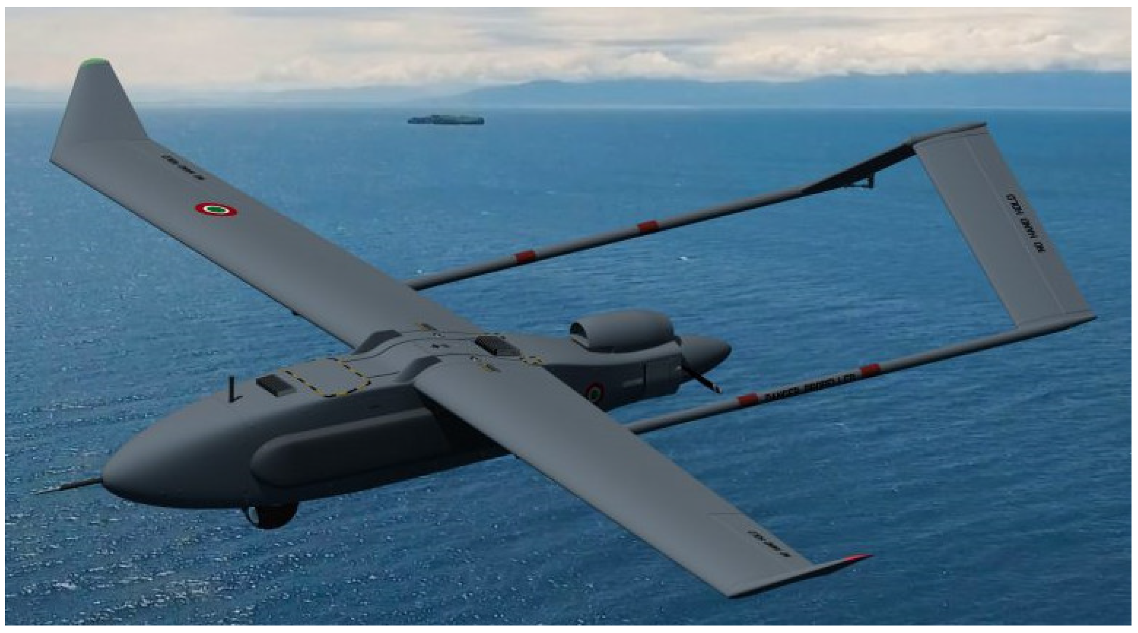
In this context, the Italian Government and the Tuscany Regional Government co-funded the project TERSA (Tecnologie Elettriche e Radar per Sistemi aeromobili a pilotaggio remoto Autonomi) [1], led by Sky Eye Systems (Italy) in collaboration with the University of Pisa and other Italian industries. The TERSA project aims to develop an Unmanned Aerial System (UAS) with a fixed-wing UAV, Figure 1, having the following main characteristics:
- Take-off weight: from 35 to 50 kg;
- Endurance: >6 h;
- Range: >3 km;
- Take-off system: pneumatic launcher;
- Landing system: parachute and airbags;
- Propulsion system: Permanent Magnet Synchronous Motor (PMSM) powering a twin-blade fixed-pitch propeller;
- Innovative sensing systems:
- ○
- Synthetic aperture radar, to support surveillance missions in adverse environmental conditions;
- ○
- Sense-and-avoid system, integrating a camera with a miniaturised radar, to support autonomous flight capabilities in emergency conditions.
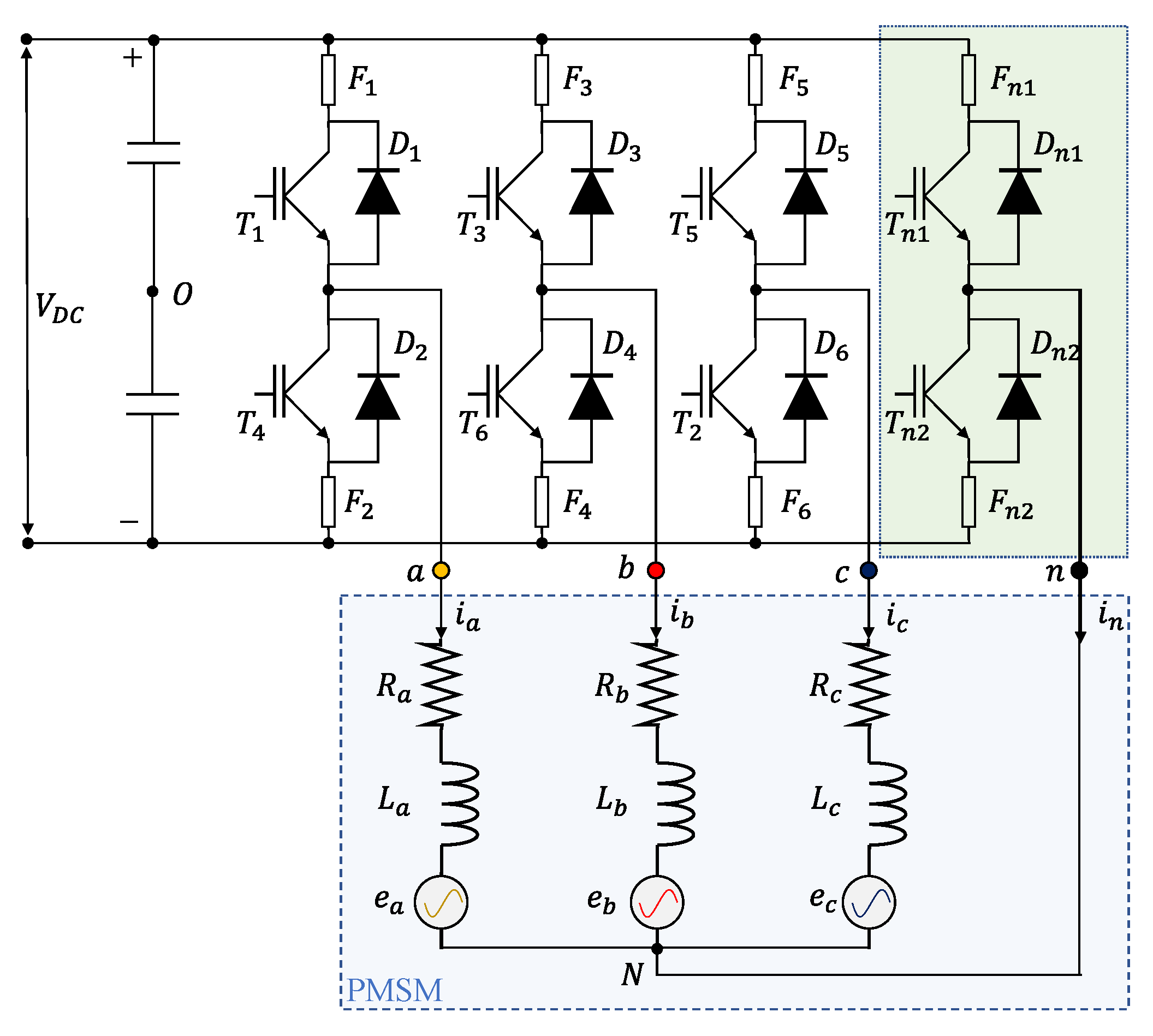
With reference to the activities related to the TERSA UAV propulsion system development (which this work refers to), a special attention has been devoted to the architecture definition for obtaining fault-tolerant capabilities. In particular, propulsion systems based on three-phase PMSMs driven by conventional three-leg converters typically have failure rates from 100 to 200 per million flight hours [2], which are not compatible with the reliability and safety levels required for the airworthiness certification [3]. The failure rate of PMSMs is mostly driven by motor phase faults and converter faults (open-switch in a converter leg, open-phase, inter-turn, phase-to-leg, phase-to-ground, or capacitor short-circuits [4]), which cover from 60% to 70% of the total fault modes [5]. Provided that the weight and envelopes required by UAV applications impede the extensive use of hardware redundancy (e.g., redundant motors), the reliability enhancement of full-electric propulsion systems can be achieved only through the redundancy of phases or stator modules [6] or by unconventional converters. By reducing design complexity, weight and envelopes, the use of four-leg converters [7,8,9], Figure 2, could represent a suitable solution for UAV applications.
In this converter topology, a couple of power switches are added, as stand-by devices, to the conventional three-leg bridge, enabling the control of the central point of the “star” connection (often Y-connection) of the motor. Nevertheless, to benefit from their fault-tolerance capability, these devices must be promptly reconfigured when a fault occurs, and extremely fast Fault-Detection and Isolation (FDI) algorithms must be developed. Especially for PMSMs operating at high speeds (such as the ones used for aircraft propellers), phase faults can generate abnormal torque ripples and the related failure transients can potentially cause unsafe conditions [10,11].
Many pieces of research on the development of FDI algorithms for PMSMs have been carried out in the last decades, and a special attention has been recently addressed to the Inter-Turn Short Circuit (ITSC) fault [12,13,14,15], which typically contributes to 10% of the PMSM failure rate [5,9,16].
Faiz [12] carried out a comprehensive literature review on FDI methods for ITSC faults in PMSMs. Depending on the measurements processed by the algorithms, they can be categorized as torque-based [17,18], flux-based [19,20], electromagnetic parameters-based [21], voltage-based, and current-based.
The most common strategy is given by the voltage-based methods. Immovilli and Bianchini [22] propose reconstructing harmonic patterns of the voltage components in the Clarke plane. The technique works very well in transient conditions, but it is not able to identify the shorted phase. The FDI algorithm proposed in [23], implements an estimator of back electromotive force and detects the ITSC by comparing the estimates to a reference model. The method is very robust against load disturbances, but it requires a very accurate model of the Back Electromotive Force (BEMF). Other approaches use as fault symptoms the harmonic components of the Zero Sequence Voltage Component (ZSVC) signal. Urresty et al. [24] proposes a Vold–Kalman Filtering Order Tracking (VKF-OT) algorithm to track the ZSVCs first harmonic component. The method offers reliable indicators, which are applicable in transient phases too, but it needs to be extended in terms of fault isolation. A robust algorithm is proposed by Hang et al., in [25], where the fault indicators are defined to remove the influence of rotor speed variation and a frequency tracking algorithm based on reference frame transformation is used to extract the fault symptoms. A possible drawback is the dependency of the fault indicator on the PMSM parameters, which may vary with environmental temperature. Boileau [26] considered as a fault indicator the amplitude of the positive voltage sequence while Meinguet [27] used as an indicator the ratio between the amplitudes of negative and positive voltage sequences. These methods are not able to locate the shorted phase, neither.
Concerning the current-based methods, the most relevant one is based on the so-called Park Vector Approach (PVA) [28,29,30,31]. When the PMSM is operating in normal conditions, the current phasor in the Clarke plane draws a circular trajectory, while it follows an elliptic one if a stator fault occurs. In PVAs, the fault index is thus defined by a geometrical distortion factor, obtained by currents measurements. Though demonstrating to be excellent for online ITSC FDI, the PVA is not able to locate the shorted phase.
All the current methods have in common the observation that in case of ITSCs, the stator currents are not balanced, and higher harmonic components in the signals can be used as fault symptoms. Different signal processing methods are employed to extract these symptoms (or patterns). Frequency-domain transforms such as Fast-Fourier Transforms (FFT) are applied in [13,32,33,34], while mixed frequency/time-domain transforms such as Short-Time Fourier Transform (STFT) are used in [14], Wavelet Transform (WT) in [15,35,36], and Hilbert–Huang Transform (HHT) in [37,38]. Frequency-domain transforms entail the loss of transient events such as speed or loads variations, so FFT analyses, though effective in stationary conditions, must be avoided if the FDI is required during transients. By requiring a higher computational effort, STFT analyses partially compensate the FFT limits, but FDI capabilities are still limited in unsteady conditions. On the other hand, WT methods permit to decompose time domain signals into stationary and non-stationary contributions, but the appropriate choice of wavelets is a drawback. Many limits of WT techniques are removed by HHT techniques, even if they are effective when applied to signals characterised by a narrow frequency content.
Other methods, based on artificial intelligence applications (Convolutional Neural Networks are used in [39]) have been also explored, but, though the results are remarkable, these techniques are not preferred for airworthiness certification [40].
Within this research context, this paper aims to develop an innovative Fault-Tolerant Control (FTC), capable of prompt FDI and accommodation of ITSC faults in three-phase PMSMs for lightweight UAVs propulsion, in both stationary and transient conditions. The proposed FTC is composed of two sections: the first one addresses the FDI problem via an original current-based method (here referred as Advanced-PVA, APVA), the second is dedicated to the fault accommodation, obtained by activating the stand-by leg of a four-leg converter and controlling the central point of the motor Y-connection. It is worth noting that the ITSC accommodation is developed by applying the Rotor Current Frame Transformation Control (RCFTC) technique, already applied by the authors in [9] for the FTC of open-circuit faults.
The paper is articulated as follows: in the first part, the nonlinear model of the propulsion system is presented; successively, the FDI algorithms and the fault accommodation technique are described by highlighting their basic design criteria; finally, a summary of the simulation results is proposed, by characterizing the failure transients and the post-fault behaviours after the injection of ITSC faults.
2. Materials and Methods
2.1. System Description
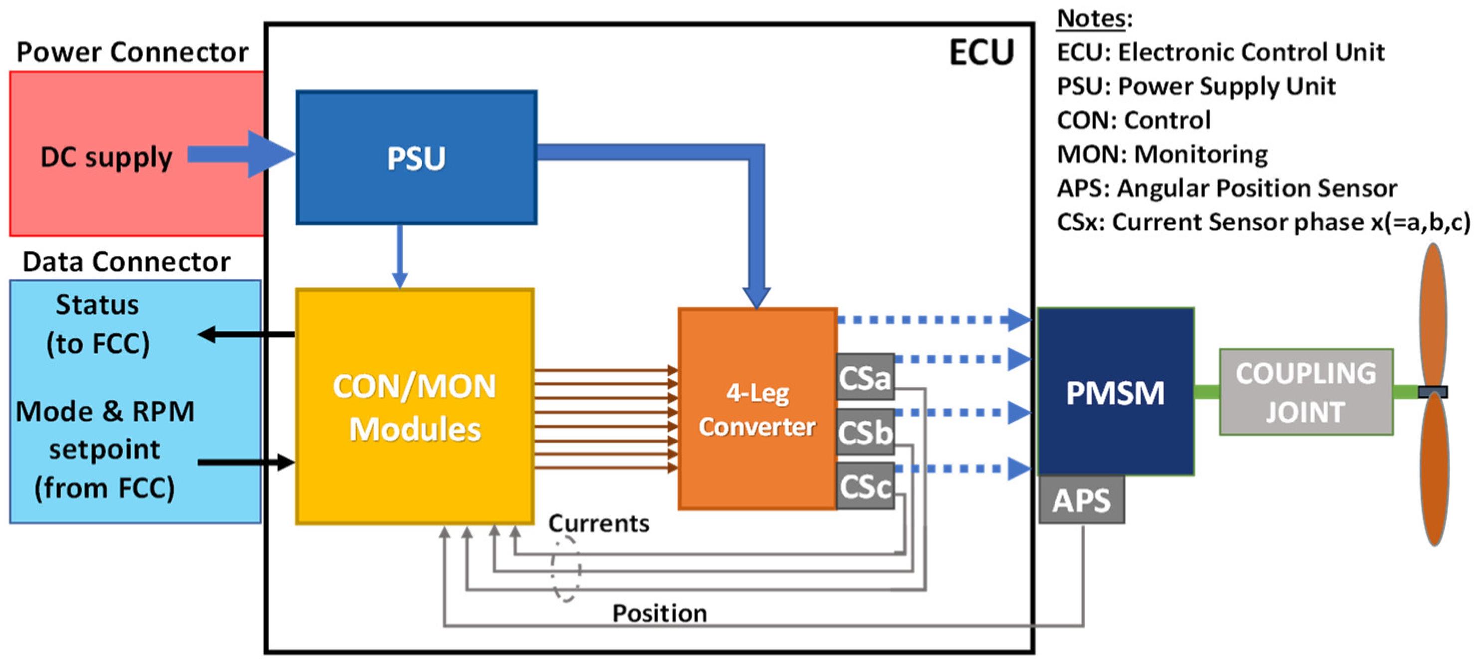
The reference propulsion system, designed for the full-electric propulsion of a lightweight UAV, is composed of (Figure 3):
- An electromechanical section, with:
- ○
- Three-phase surface-mounted PMSM with phase windings in Y-connection;
- ○
- Twin-blade fixed-pitch propeller [41];
- ○
- Mechanical coupling joint.
- An Electronic Control Unit (ECU), including:
- ○
- CONtrol/MONitoring (CON/MON) module, for the implementation of the closed-loop control and health-monitoring functions;
- ○
- Four-leg converter;
- ○
- Three current sensors (CSa, CSb, CSc), one per each motor phase;
- ○
- One Angular Position Sensor (APS), measuring the motor angle;
- ○
- A Power Supply Unit (PSU), converting the power input coming from the UAV electrical power storage system to all components and sensors;
- ○
- Data and power connectors for the interface with the Flight Control Computer (FCC) and the UAV electrical system.
The CON module operates the closed-loop control of the system by implementing two nested loops on propeller speed and motor currents (via Field-Oriented Control, FOC). All the regulators implement proportional/integral actions on the tracking error signals, plus anti-windup functions with back-calculation algorithms to compensate for commands saturation. The MON module executes the health-monitoring algorithms, including the FTC proposed in this work.
2.2. Model of the Aero-Mechanical Section
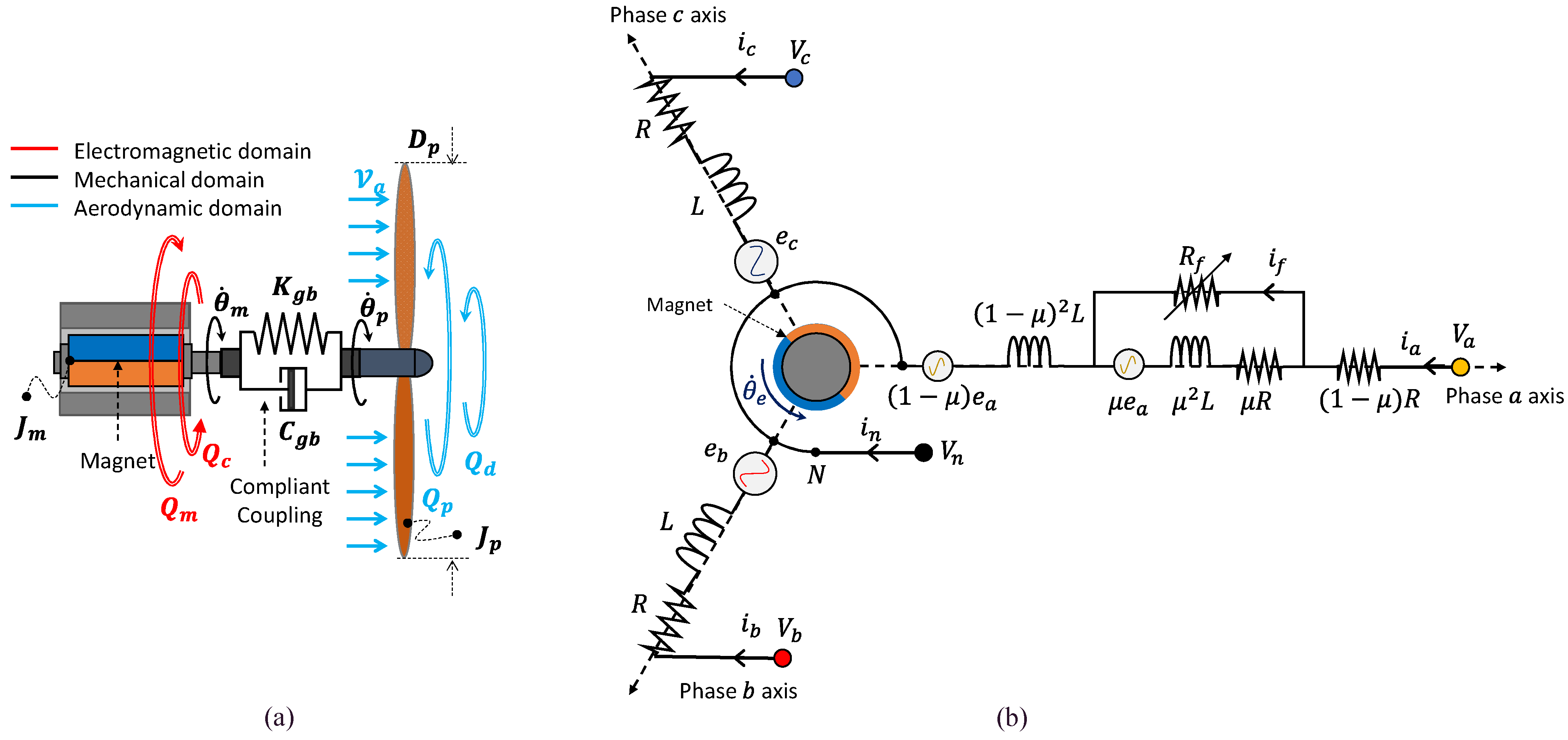
The dynamics of the aero-mechanical section of the propulsion system, providing the UAV with the thrust is schematically depicted in Figure 4a and is modelled by [7,9]:
where and , , and are the inertia and the angular position of the propeller and the motor, respectively, is the propeller-resistant torque, is a gust-induced disturbance torque, is the motor torque, , is the cogging torque, and is the maximum cogging torque, is the pole pairs number, is the harmonic index of the cogging disturbance, is the nondimensional torque coefficient of the propeller, is the propeller advance ratio, is the propeller diameter, is the air density, is the UAV forward speed, while and are the stiffness and the damping of the mechanical coupling joint.
2.3. Model of the PMSM with ITSC Fault
The mathematical modelling of PMSM with ITSC faults that will be used for this work has been previously presented and applied in literature, demonstrating it to be very accurate [13,42,43,44].
The occurrence of a short circuit in a stator phase causes an asymmetry in the motor magnetic flux, due to an additional circuit with insulation resistance , in which the shorted current flows, Figure 4b:
Once indicated, the fault extension along the winding with the parameter (defined as the ratio of the number of shorted turns to the total one), the winding affected by ITSC can be split into an undamaged and a damaged part, Figure 4b. Hence, the electrical equations can be written as:
In Equation (2), is the applied voltages vector, is the currents vector, e is the BEMF vector, which can be expressed as in Equation (3) (in Equation (3) and in the following equations, “s” and “c” briefly indicates “sine” and “cosine” functions):
where is the electrical angle of the motor and is the rotor magnet flux linkage. The resistance and inductance matrixes are:
in which is the phase resistance, is the phase self-inductance, and is the insulation resistance, given by:
with a factor depending on the insulation material.
By considering an inter-turn fault, the PMSM torque can be calculated as [44]:
Since the neutral point voltage is not null when a short circuit occurs, it is convenient to reformulate the electrical equations by extrapolating . Hence, by applying Kirchhoff laws to the circuit in Figure 4b and by substituting in Equation (2), we have:
where the reformulated BEMF vector is:
The new resistance and inductance matrixes are:
while is a vector defining the voltage commands sent by the converter to the motor terminals (first three components) and the voltage on the shorted turns. Finally, since the PMSM is controlled via FOC technique, it is convenient to express the voltage vector via the Clarke–Park transformation, as a function of direct and quadrature voltages and , generated by the closed-loop control algorithms:
3. Fault-Tolerant Control System
3.1. FDI Algorithm Conceptualization
When a PMSM operates at constant speed without faults, the current phasor in the Clarke plane draws a circular trajectory, while it follows an elliptical trajectory when an ITSC fault occurs [28,29,30,31]. Torque oscillations appear, at the motor level, with amplitudes that depend on the short-circuit extension.
This section aims to demonstrate that the geometrical parameters of this elliptical trajectory (major, minor axes length, and axes inclination) are univocally related to the location and extension of the ITSC. In particular, we will demonstrate that:
- An ITSC fault can be detected by measuring the difference between the lengths of major and minor axes of the ellipse;
- An ITSC fault can be isolated by measuring the inclination of the major axis of the ellipse.
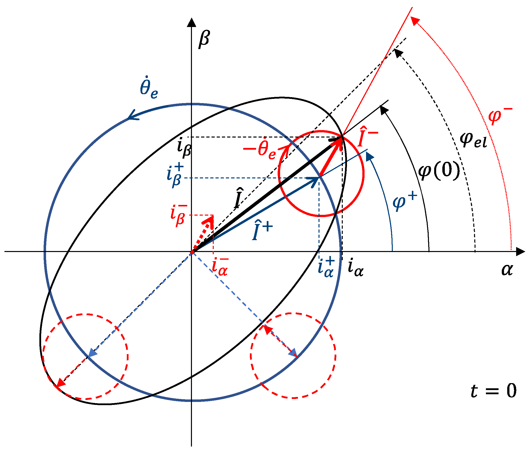
It is worth noting that, during constant speed operations, any elliptical trajectory of the motor current phasor in the Clarke plane (including the circular one, as a special case) can be reconstructed via the Fortescue decomposition [45], as the sum of three symmetrical and balanced rotating systems: positive-, negative-, and zero-sequence systems.
When an ITSC fault occurs, the central point of the Y-connection is isolated, so the zero-sequence current is zero, and the ellipse tracked by the current phasor () can be considered as the sum of two counter-rotating phasors: positive- () and negative-sequence phasors (), as given by:
where , , and are the phase angles of the resultant, positive-, and negative-sequence current phasors, respectively. As illustrated in Figure 5, the semi major and semi minor axis lengths are obtained by:
While the inclination of the ellipse major axis corresponds to the angle that maximizes the current phasor amplitude, up to:
The condition in Equation (13) is reached when the positive- and negative-sequence phasors have the same angular orientation:
which leads to:
To identify the ellipse inclination, it is thus crucial to evaluate the phase angles of the positive- and negative-sequence phasors, expressed by:
where “” stands for “” or “”, and and are the projections of the phasor on the and axes in the Clarke plane.
By introducing a complex analysis notation, the phasor can be also represented in terms of a balanced three-phase space vector system, as:
Then, by expressing the space vector into its real () and imaginary () components, we have:
The phase angles of the positive- and negative-sequence phasors with ITSC faults can be thus calculated via the positive- and negative-sequence phasors related to phase a only ( and ), given by the Fortescue transform:
The vector of phasors can be obtained from:
where the voltage and BEMF phasors are:
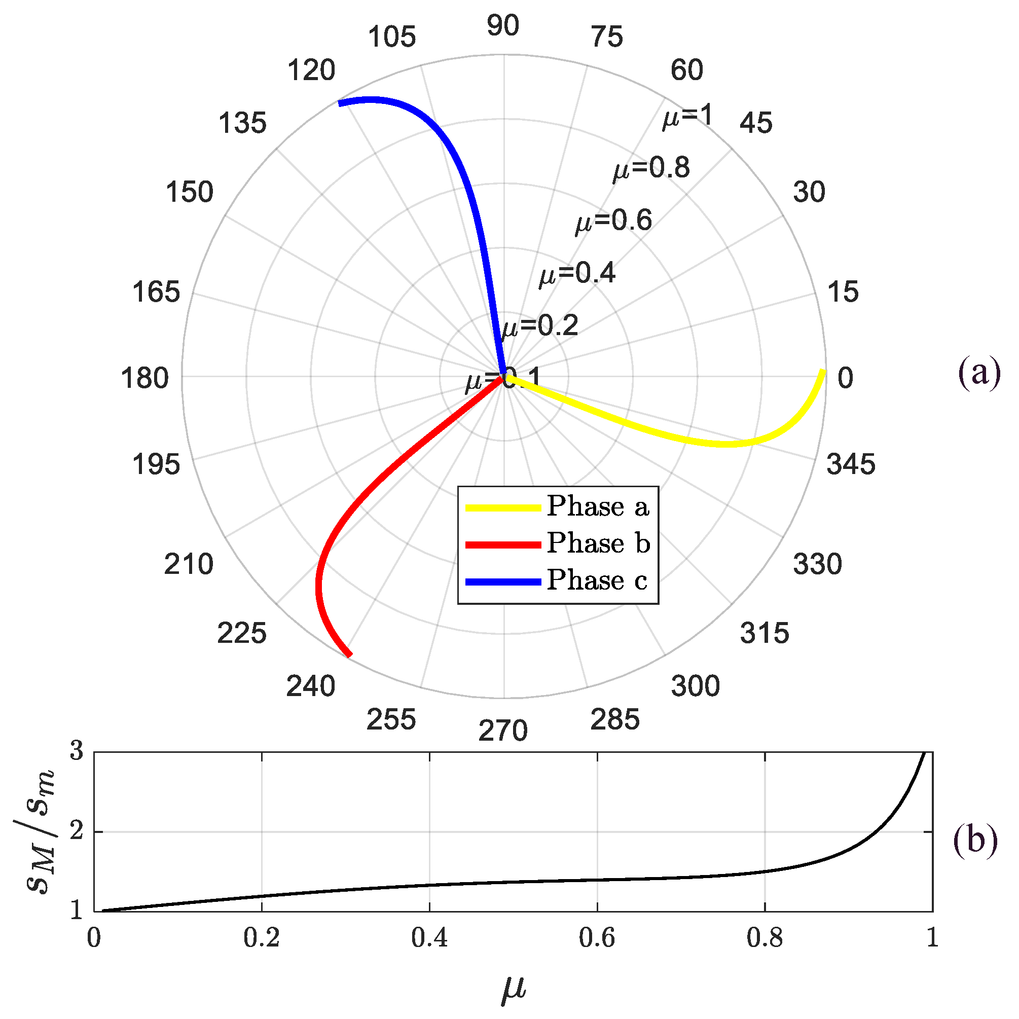
The solution of Equation (20) in terms of current phasors are presented by the polar-coordinate plot in Figure 6a, in which, given along the radius the ITSC fault extension (), the inclination of the ellipse major axis of the current phasor trajectory is reported along the phase angle for each motor phase. In addition, Figure 6b shows the ratio of ellipse semi-axes lengths as a function of the ITSC fault extension parameter . It is worth noting that, if an ITSC fault occurs on phase a (b, c), the ellipse inclination will be 0° (240°, 120°) ±15°.
The above-mentioned discussion thus supports the development of an FDI algorithm based on the estimation of the geometrical characteristics of (generic) elliptical trajectories of current phasors in the Clarke plane, so that:
- The difference between the lengths of major and minor axes of the ellipse provides a symptom about the ITSC extension (fault detection);
- The inclination of the major axis of the ellipse provides a symptom about the ITSC location (fault isolation).
The FDI concept essentially entails the identification of geometrical properties of an ellipse. Clearly, at a single monitoring time, a single point of the ellipse is known ( Figure 5); therefore, the fitting problem is under-determined. On the other hand, the problem becomes over-determined if a sufficient number of measurements are used. The over-determined problem of fitting an ellipse to a set of data points arises in many applications such as computer graphics [46], hydraulic engineering [47], and statistics [48]. Many different methods are proposed in literature for fitting the geometric primitives of an ellipse: voting/clustering methods (e.g., the Hough transform [49] and the RANSAC technique [50]) are robust but they have poor accuracy and require large computing resources, optimization methods and direct least-square methods [51] are accurate, but, in case of nonlinear applications such as an ellipse fitting, they apply iterative techniques.
Here we instead use a direct least-square method, as proposed by Halìř and Flusser [52], who, starting from the quadratically-constrained least-squares minimization postulated by Fitzgibbon [53], reformulated the problem via partitioning techniques, by obtaining a very robust and computationally-effective algorithm.
Once given the vectorial conic definition of an ellipse,
in which and are vectors defining the Cartesian coordinates of the ellipse points and the ellipse coefficients, respectively, the over-determined fitting problem to a set of coordinate points and (where , and is greater than the number of ellipse coefficients, i.e., > 6) can be solved by the following eigenvalues problem (for more details, see Appendix A):
where is the reduced scatter matrix,
with the ellipse coefficient vector segmented in and . The solution of Equation (24) corresponds to the eigenvector yielding a minimal non-negative eigenvalue . Once obtained , the lengths of major and minor semi-axes and are given by [54]:
while the major axis inclination is [54]:
3.2. FDI Algorithm Design and Implementation
One of the basic limitations of the proposed FDI concept is that the technique is defined by assuming constant speed motor operations. During unsteady conditions, the current phasor changes its amplitude while rotating in the Clarke plane. Consequently, the ellipse identification does not work appropriately, and it could cause false alarms.
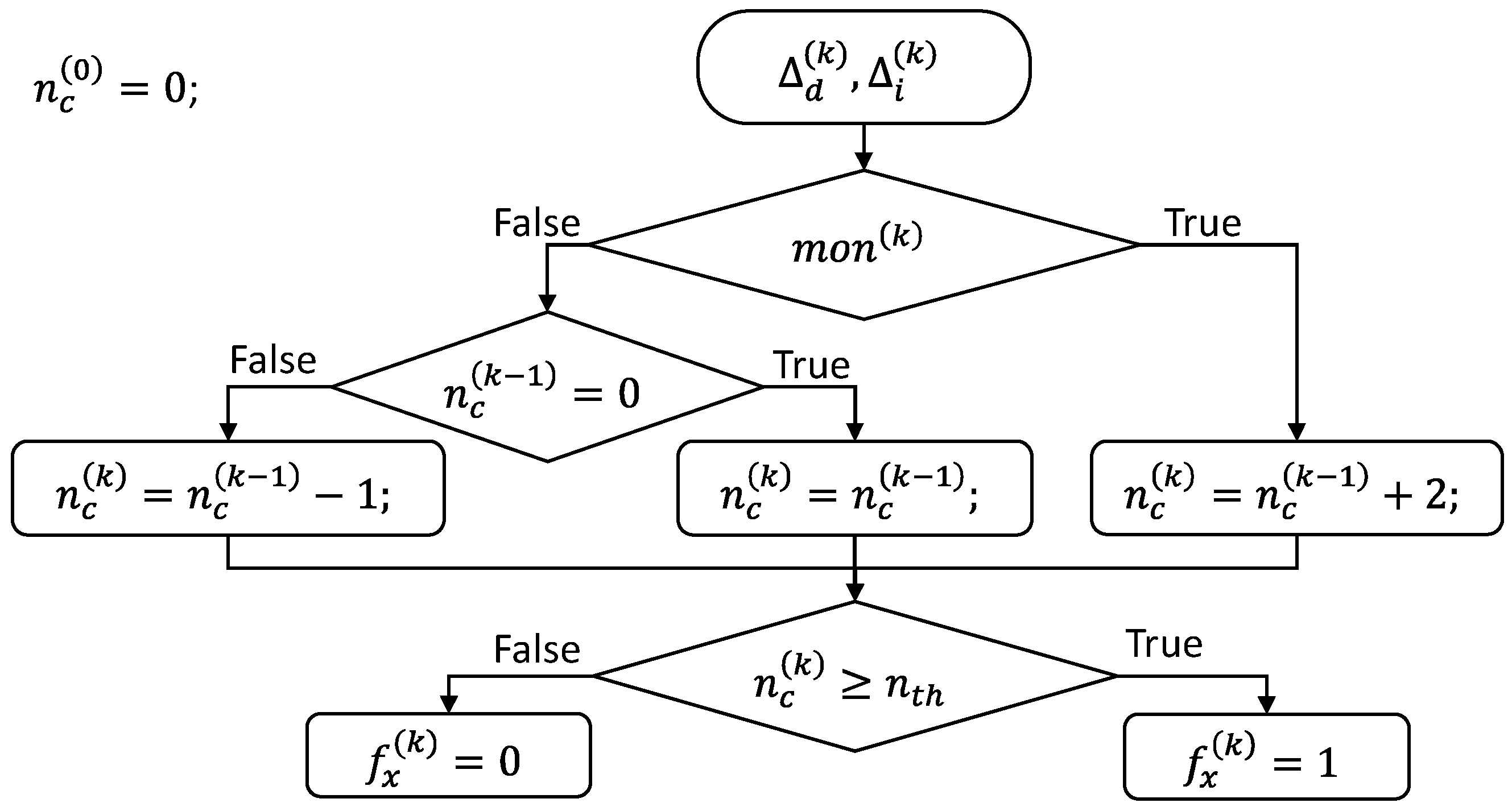
To overcome the problem, it is worth noting that, differently from the constant speed operations with ITSC faults, the axes of the ellipse reconstructed in unsteady conditions rotate. For this reason, the developed FDI algorithm detects an ITSC fault only if the value of the ellipse major axis is constant and stationary. This FDI logic has been implemented as represented by the flow chart in Figure 7: at each k-th monitoring sample, if the Boolean variable is true (Equation (32)), a fault counter is increased by two, otherwise it is reduced by one. When the fault counter reaches a predefined maximum value (), the algorithm outputs a true Boolean fault flag , which indicates that a fault on the phase is detected and isolated.
where:
The details and a dedicated discussion about the FDI parameters design are proposed in Section 4, while tables reporting the FDI parameters are reported in Appendix B.
3.3. Fault Accommodation Algorithm
After the FDI algorithm detects and isolates the ITSC fault, the motor still has two active phases. To maintain the performances after the fault, the FTC should accommodate the system by restoring the operation of the current phasor in the Clarke plane as it was in healthy conditions. This is here achieved by enabling the control of the central point of the motor Y-connection, via the stand-by leg of the four-leg converter, and by applying an RCFTC technique [9,55].
To maintain the torque performances with only two phases, the currents amplitudes in the healthy phases in the rotor reference frame ( ) must increase by w.r.t. those before the fault, and they must shift by 60° along the electrical angle. In addition, the amplitude of the current flowing into the central point () must be times those in the healthy phases:
In Equation (36), are the current demands in the Park frame before the fault. The subscripts , , and indicate the healthy and the isolated phases, while is an integer number defined by the values in Table 1.
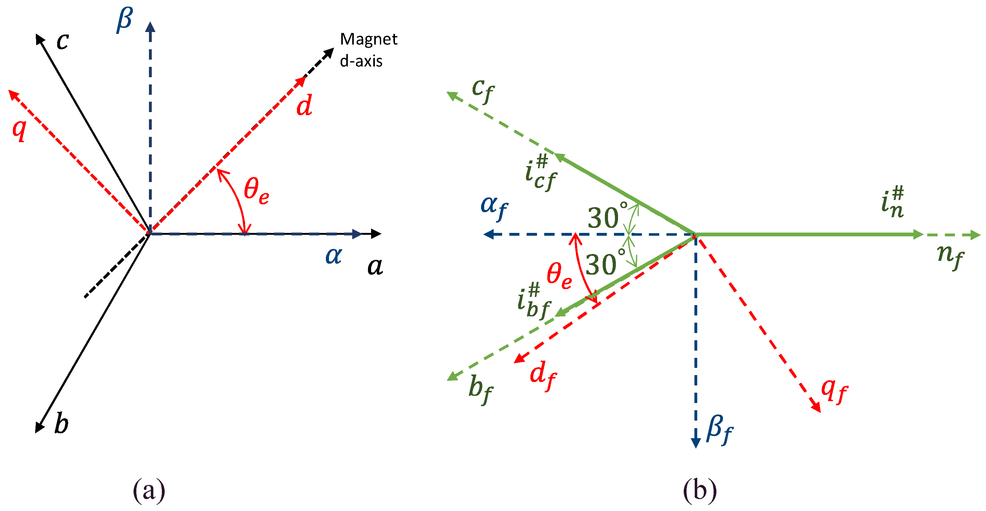
Since all the current demands in the stator frame are synchronous with the rotor motion, they can be expressed into a rotating frame by applying two new Clarke–Park transformations [9,55] (Figure 8):
- From the planar reference to a planar reference frame , in which the axis has an opposite direction w.r.t. the neutral current axis ;
- From the planar reference to a planar rotating frame that maintains the same commands after the isolation ( and .
The RCFTC accommodation is finally completed by inverting the direct transformation matrix to calculate the reference voltages for the converter:
where
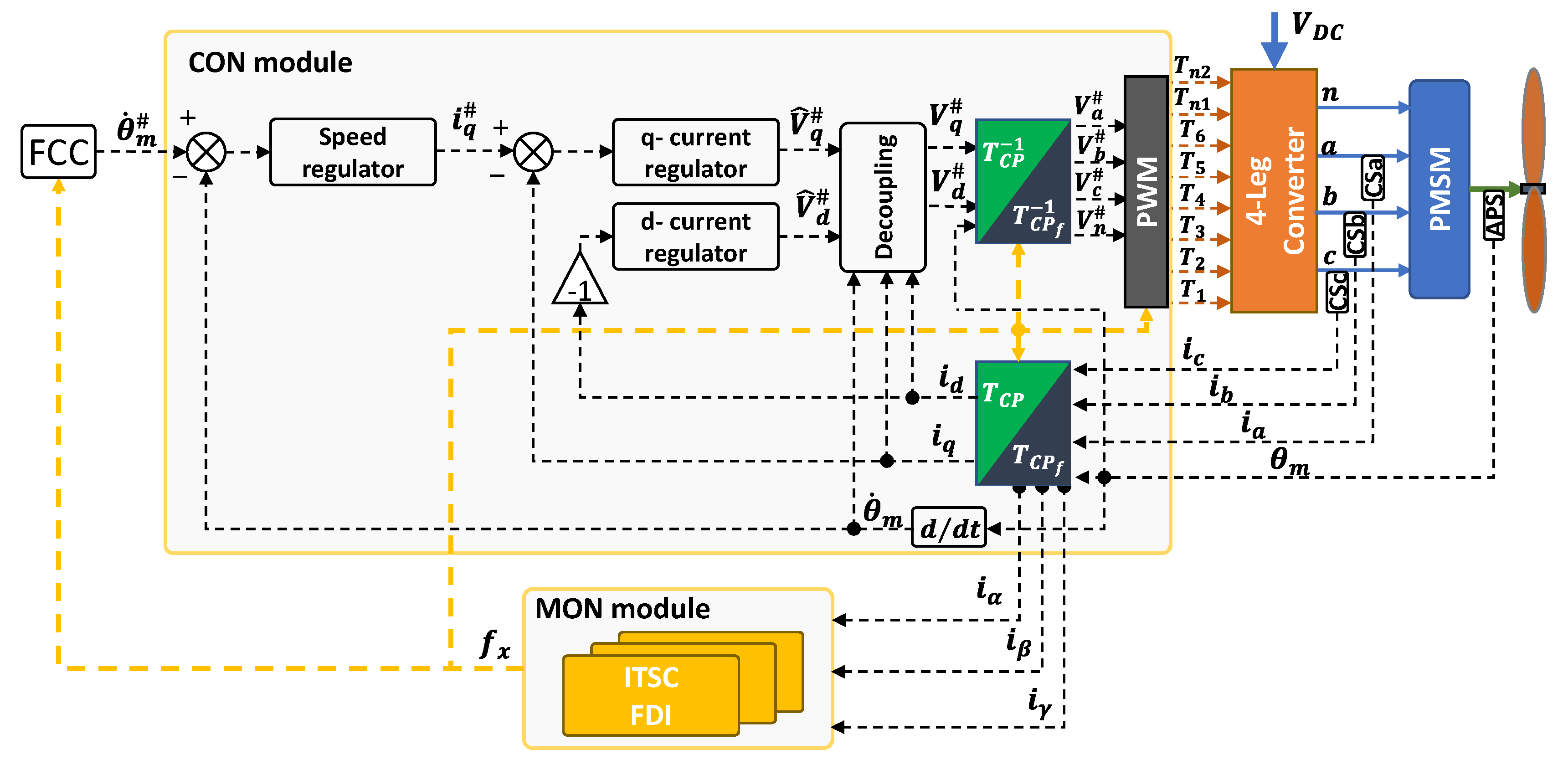
The integration of the proposed FTC strategy within the motor closed-loop system is schematically depicted in Figure 9.
When the system is in normal condition, the conventional Clarke–Parke transformations are employed () and the central point of the Y-connection is isolated ( and are not used). Once an ITSC is detected and isolated, the reference frame transformations of the RCFTC are employed (), and the reconfigured voltage references are sent to the four-leg converter to signal the central point ( and ).
4. Results and Discussion
4.1. Failure Transient Characterization
The effectiveness of the presented FTC strategy has been tested by using the nonlinear model of the propulsion system. The model is entirely developed in the MATLAB/Simulink environment, and its numerical solution is obtained via the fourth order Runge–Kutta method, using a 10−6 s integration step. It is worth noting that the choice of a fixed-step solver is not strictly related to the objectives of this work (in which the model is used for “off-line” simulations testing the FTC), but it has been selected for the next step of the project, when the FTC system will be implemented in the ECU boards via the automatic MATLAB compiler and executed in “real-time”.
The closed-loop control is executed at a 20 kHz sampling rate and the maximum allowable fault latency has been set to 50 ms (for details, see Section 4.2). All the simulations started (t = 0 s) with a healthy PMSM, driving the propeller at 5800 rpm (UAV in straight-and-level flight at sea level Table A1).
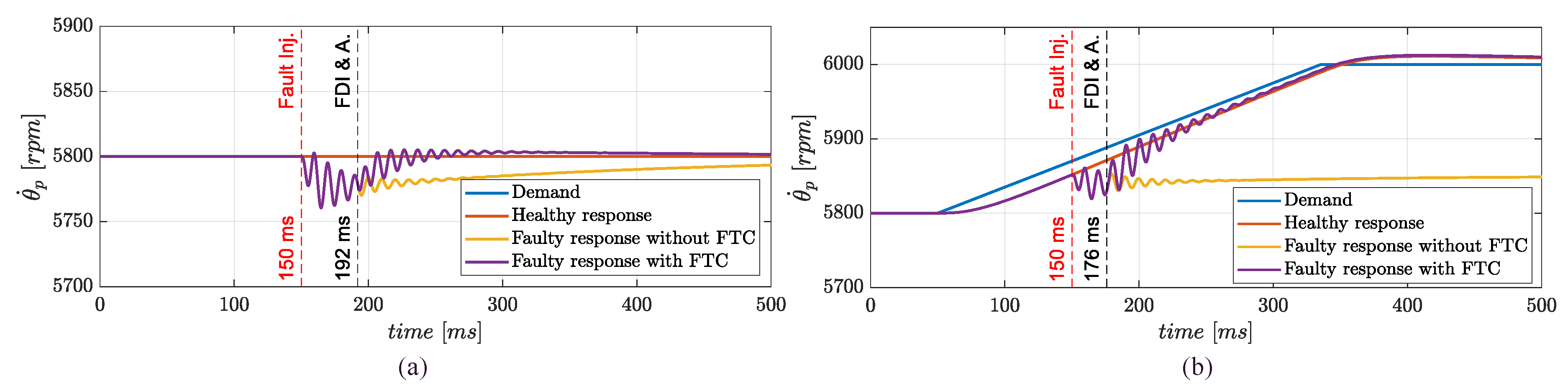
The FTC strategy has been assessed by simulating the occurrence of an ITSC fault with on phase a at t = 150 ms. The failure transient is characterized by applying or not the proposed FTC and by comparing the responses with those in healthy conditions. As shown by Figure 10, though its relevant extension, the ITSC fault implies minor impacts on the propeller speed response during stationary operations (Figure 10a), even if the FTC application assures a faster recovery of the pre-fault speed value. On the other hand, the failure transient during unsteady operations is much more limited with FTC, even if small-amplitude ripples (at approximately 100 Hz) appear immediately after the accommodation (Figure 10b). These responses highlight the importance of applying the FTC for ITSC faults: since the fault effects are minor during stationary operations, its detection is very difficult, but the ITSC is typically unstable, and it progressively spreads along the phase windings if the coil is not isolated.
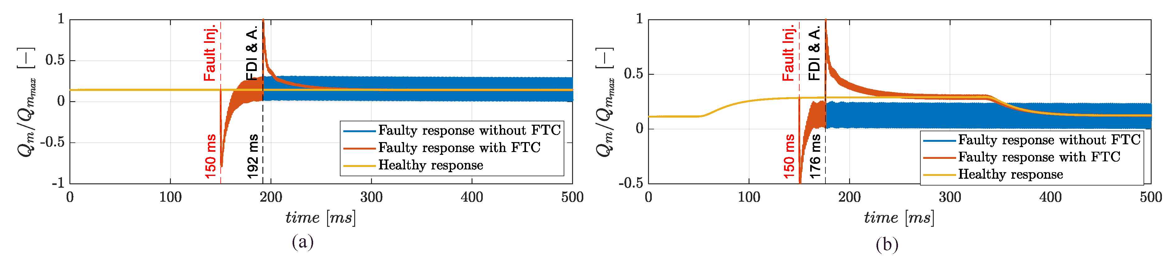
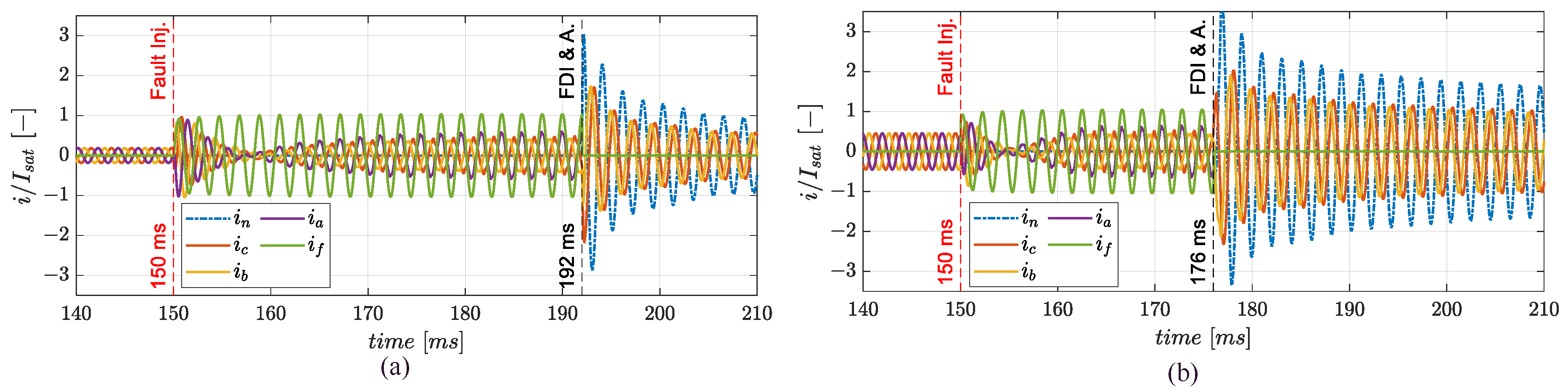
The failure transient in terms of motor torque is then reported in Figure 11. It can be noted that, if the FTC is not applied, the post-fault behaviour is characterized, during both stationary and unsteady operations, by relevant high-frequency ripples (at approximately 1 kHz, i.e., twice the electrical frequency of the motor). In particular, during stationary operations, the FTC permits to rapidly restore the pre-fault torque level, by eliminating high-frequency loads that would inevitably cause damages at mechanical and electrical parts (Figure 11a). The failure transients in terms of phase currents are then reported in Figure 12, when the FTC is applied. The fault generates a short circuit current (, Figure 12) causing the loss of symmetry of the three-phase system. Thanks to the RCFTC accommodation, the phase a is disengaged and the fourth leg of the converter is activated: this action stops the short circuit current and opens a current path through the central point (, Figure 12).
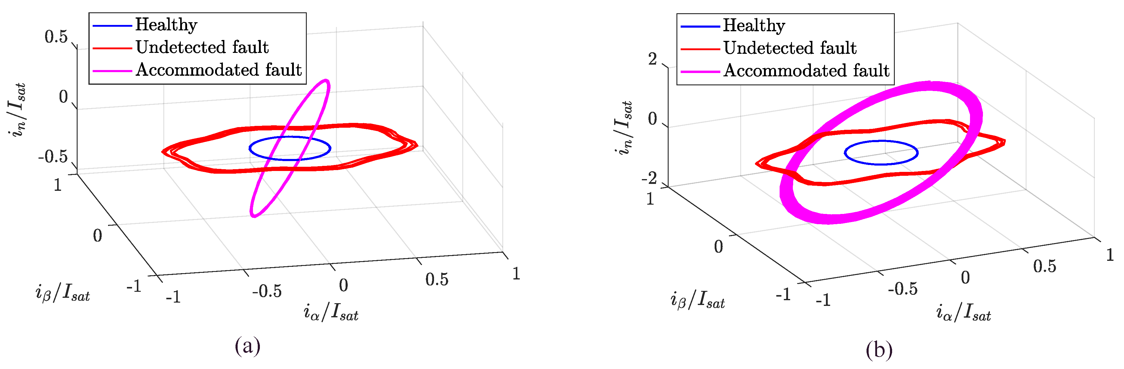
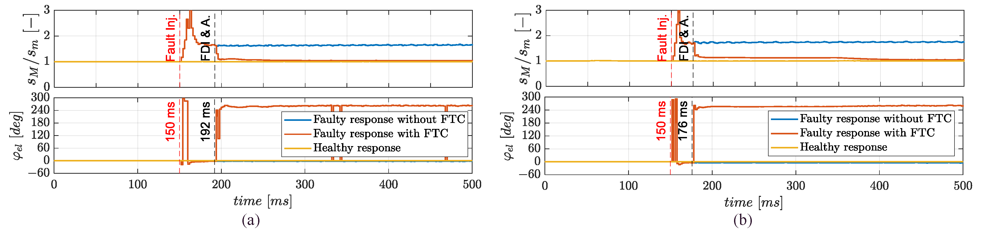
The current phasor trajectories in the Clarke space are shown in Figure 13. It can be noted that, when an ITSC fault is injected in phase a, the trajectories are not strictly elliptical. This depends on the fact that the faulty currents are not perfectly sinusoidal, but they also contain higher harmonic contents. The phenomenon is caused by the phase voltages saturation. Despite the presence of these higher harmonic contents, the ellipse fitting technique successfully operates by demonstrating the relevant robustness of the FDI algorithm. On the other hand, when the fault is accommodated, the trajectory involves the neutral axis too, in such a way that, its projection on the plane overlaps the healthy circular trajectory. Finally, the geometrical parameters of the current phasor elliptical trajectory (semi-axes lengths and major axis inclination) are plotted in Figure 14. It can be noted that, when the FTC intervenes, the projection of the current trajectory on the plane becomes circular () and the ellipse inclination returns to zero.
4.2. FDI Parameters Definition
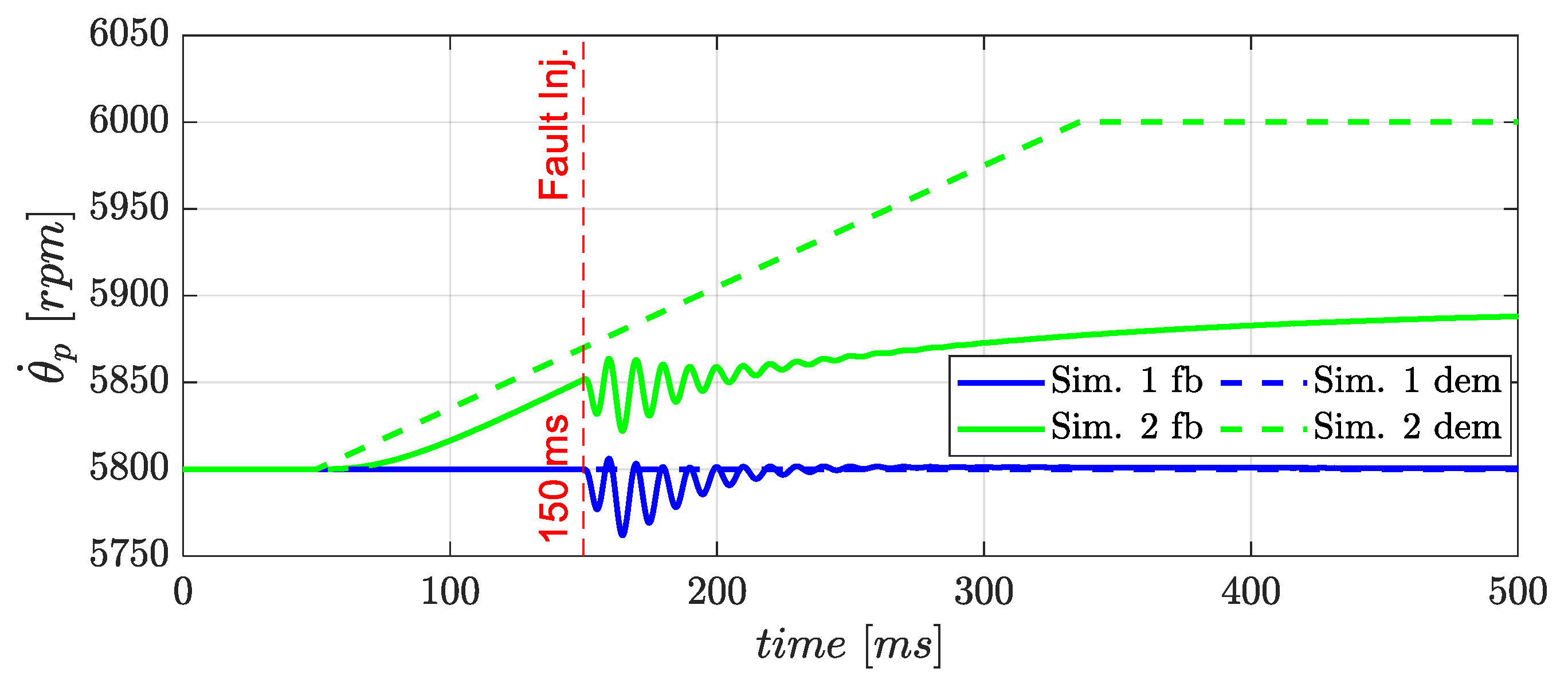
As described in Section 3.2, the design of the FDI algorithm requires the definition of four parameters, i.e., , , , and . Concerning the ellipse fitting samples , this parameter has been defined by pursuing a good balance between the trajectory reconstruction accuracy and the FDI latency, both increasing when increases. Considering that the propeller speed tracking bandwidth is approximately 15 Hz, the maximum allowable FDI latency has been set to 50 ms, which could be reasonably targeted by an equivalent monitoring frequency of 500 Hz. Being the sampling rate of the sensor system at 20 kHz, has been imposed. The values of the remaining parameters (, , ) have been instead defined via time domain simulations, aiming to obtain correct ITSC FDI with very limited extension (). Two FDI design simulations have been performed, Figure 15:
- Simulation 1: cruise speed hold,
- Simulation 2: maximum speed ramp demand.
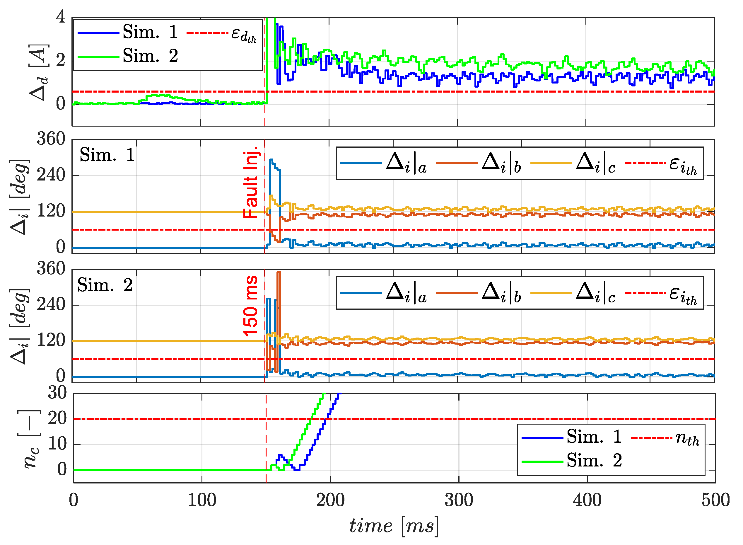
The FDI parameter plotted in Figure 16 shows that low values of would clearly imply a too-sensitive algorithm, with high counts during unsteady operations and in turn high values of to avoid false alarms. On the other hand, high values of will make the algorithm too robust to false alarms but it will reduce the effectiveness in detecting ITSC at an early stage. In the proposed case study, a good balance between the robustness against false alarms and the effectiveness in diagnosing ITSC higher than can be obtained by selected and , which guarantees an FDI latency lower than the 50 ms among the two cases reported in Figure 15.
4.3. Critical Comparison with Other ITSC FDI Methods
A comparative analysis of the proposed FDI method with the most relevant ones developed in the literature (Table 2) has been carried out by using the list of capabilities given in Table 3. The results are reported in Table 4.
The FFT methods are robust against noise, but they are not applicable in unsteady operations. They can be enhanced by applying HHT transforms, but the capability to detect the faulty phase is lost. Similarly, the main disadvantage of the PVA methods is the inability to locate the fault. The CNN method is competitive in terms of the ITSC location, but their robustness in unsteady operations has not been proved; furthermore, the design of the neural detector requires a complex design and training process. On the other hand, the proposed APVA method demonstrates excellent capabilities in unsteady operations, it succeeds in fault location and detects ITSC faults with a very limited extension (10%, less than four turns) independently from the load level. All the methods considered are capable of detecting incipient faults, but many of them lack enough information for a comparison in terms of detection and isolation latency.
5. Conclusions
A novel FTC strategy for a high-speed PMSM with a four-leg converter employed for UAV propulsion is developed and characterized in terms of FDI and fault accommodation capabilities. The FTC performances are assessed via dynamic simulation by using a detailed nonlinear model of the electric propulsion system, which includes a physically based modelling of ITSC faults. For the proposed FTC, an original FDI algorithm is developed and applied, based on an innovative current signature technique, which uses as fault symptoms the geometrical parameters of the elliptical trajectory of the currents phasor in the Clarke plane (e.g., major and minor axes lengths, and major axis inclination). In addition, a theoretical analysis is carried out to support the FDI algorithms, by demonstrating that the major axis inclination can be used as a symptom for the faulty phase identification.
A comparative analysis with other ITSC FDI methods from the literature is also carried out. If compared with neural networks methods, which exhibit the best sensibility to incipient faults (a shorted turn is isolated within 10 electrical periods), the proposed technique behaves slightly worse (four shorted turns, corresponding to a 10% extension along the coil, and are isolated within 20 electrical periods). Nevertheless, the neural methods are more complicated to be tuned (due to the training process), while the proposed method only requires tuning four parameters. Finally, the paper demonstrates that a fault accommodation based on the RCFTC technique succeeds in minimizing the failure transient and eliminates the high-frequency torque ripples induced by the fault.
Author Contributions
Conceptualization, methodology and investigation, A.S. and G.D.R.; software, data curation and writing—original draft preparation, A.S.; validation, formal analysis and writing—review and editing, G.D.R.; resources, supervision and visualization, G.D.R. and R.G.; project administration and funding acquisition, R.G. All authors have read and agreed to the published version of the manuscript.
Funding
This research was co-funded by the Italian Government (Ministero Italiano dello Sviluppo Economico, MISE) and by the Tuscany Regional Government, in the context of the R&D project “Tecnologie Elettriche e Radar per SAPR Autonomi (TERSA)”, Grant number: F/130088/01-05/X38.
Institutional Review Board Statement
Not applicable.
Informed Consent Statement
Not applicable.
Data Availability Statement
Not applicable.
Acknowledgments
The authors wish to thank Luca Sani, from the University of Pisa (Dipartimento di Ingegneria dell’Energia, dei Sistemi, del Territorio e delle Costruzioni), for the support in the definition of the PMSM model parameters, and Francesco Schettini, from Sky Eye Systems (Italy), for the support in the definition of the UAV propeller loads.
Conflicts of Interest
The authors declare no conflict of interest.
Appendix A
The general ellipse expression is defined by an implicit second-order polynomial with specific constraints on coefficients.
in which and are the ellipse coefficients, while and are the Cartesian coordinates of the ellipse points. The related vectorial conic definition is:
where and .
The ellipse fitting to a set of coordinate points , coming from monitoring measurements (where , and is greater than the number of conic coefficients, i.e., > 6) is an over-determined problem, which can be approached by minimizing the sum of distances of the points to the conic represented by coefficients :
Due to the constraint, the problem cannot be solved directly with a conventional least-square approach. However, Fitzgibbon [53] showed that under a proper scaling, the inequality in Equation (A3) can be changed into an equality constraint as,
This minimization problem can be conveniently formulated as:
where and are known as the design and constraint matrices, respectively, defined as
and it can be solved as a quadratically-constrained least-squares minimization by applying Lagrange multipliers, as:
where is the scatter matrix, defined as:
The optimal solution of Equation (A7) is the eigenvector corresponding to the minimum positive eigenvalue . It is worth noting that the matrix is singular, and is also singular if all data points lie exactly on an ellipse. Because of that, the computation of eigenvalues is numerically unstable and it can produce wrong results (as infinite or complex numbers). To overcome the drawback, Halìř [52] suggested to partition the and matrices. The constraint matrix is defined as:
and
The partition of matrix is obtained by splitting the matrix into its quadratic and linear parts:
where
Then, the scatter matrix is constructed as:
in which
Similarly, the coefficients vector is partitioned as:
where
Based on this decomposition, Equation (A7) can be written as:
Considering that matrix is singular only if all the points lie on a line [52], the second of equation in Equation (A17) can be solved to obtain . By substituting in Equation (A17), and by considering that is not singular, we have:
in which is the reduced scatter matrix:
The optimal solution corresponds to the eigenvector that yields a minimal non-negative eigenvalue . Once obtained , the lengths of major and minor semi-axes and are [54]:
while the major axis inclination is [54]:
Appendix B
This section contains tables reporting the parameters of the UAV propeller (Table A1), the simulation model of the propulsion system (Table A2), and the design parameters of the FTC system (Table A3).

Table A1.
APC 22 × 10E Propeller data.
| Definition | Symbol | Value | Unit |
|---|---|---|---|
| Cruise speed | |cruise | 5800 | rpm |
| Cruise power | Pp|cruise | 1100 | W |
| Climb speed | |climb | 7400 | rpm |
| Climb power | Pp|climb | 3238 | W |
Table A2.
System model parameters.
| Definition | Symbol | Value | Unit |
|---|---|---|---|
| Stator phase resistance | R | 0.025 | Ω |
| Stator phase inductance single module | L | 1 × 10⁻⁵ | H |
| Pole pairs number | nd | 5 | - |
| Total turns number per phase | N | 36 | - |
| Torque constant | kt | 0.12 | Nm/A |
| Back-electromotive force constant | ke | 0.036 | V/(rad/s) |
| Permanent magnet flux linkage | λm | 0.008 | Wb |
| Maximum current (continuous duty cycle) | Isat | 80 | A |
| Voltage supply | VDC | 36 | V |
| Rotor inertia | Jem | 8.2 × 10⁻³ | kg·m2 |
| Propeller diameter | Dp | 0.5588 | m |
| Propeller inertia | Jp | 1.62 × 10⁻² | kg·m2 |
| Joint stiffness | Kgb | 1.598 × 10³ | Nm/rad |
| Joint damping | Cgb t | 0.2545 | Nm/(rad/s) |
| Insulation resistance coefficient | kRf | 11 | - |
| Maximum cogging torque | Qcmax | 0.036 | Nm |
| Harmonic index of the cogging disturbances | nh | 12 | - |
Table A3.
FTC Algorithm parameters.
| Definition | Symbol | Value | Unit |
|---|---|---|---|
| Control frequency | |||
| Ellipse measurement points | |||
| Sampling frequency | |||
| Detection index threshold | |||
| Isolation index threshold | |||
| Fault counter threshold |
References
- Dipartimento di Ingegneria Civile e Industriale, Progetti istituzionali. TERSA (Tecnologie Elettriche e Radar per Sistemi aeromobili a pilotaggio remoto Autonomi). Available online: https://dici.unipi.it/ricerca/progetti-finanziati/tersa/ (accessed on 1 July 2022).
- Nandi, S.; Toliyat, H.; Li, X. Condition Monitoring and Fault Diagnosis of Electrical Motors—A Review. IEEE Trans. Energy Convers. 2005, 20, 719–729. [Google Scholar] [CrossRef]
- NATO Standardization Agency. STANAG 4671—Standardization Agreement—Unmanned Aerial Vehicles Systems Airworthiness Requirements (USAR); NATO Standardization Agency (STANAG): Brussels, Belgium, 2009. [Google Scholar]
- Kontarcek, A.; Bajec, P.; Nemec, M.; Ambrožic, V.; Nedeljkovic, D. Cost-Effective Three-Phase PMSM Drive Tolerant to Open-Phase Fault. IEEE Trans. Ind. Electron. 2015, 62, 6708–6718. [Google Scholar] [CrossRef]
- Cao, W.; Mecrow, B.; Atkinson, G.; Bennett, J.; Atkinson, D. Overview of Electric Motor Technologies Used for More Electric Aircraft (MEA). IEEE Trans. Ind. Electron. 2012, 59, 3523–3531. [Google Scholar] [CrossRef]
- Suti, A.; Di Rito, G.; Galatolo, R. Fault-Tolerant Control of a Dual-Stator PMSM for the Full-Electric Propulsion of a Lightweight Fixed-Wing UAV. Aerospace 2022, 9, 337. [Google Scholar] [CrossRef]
- De Rossiter Correa, M.; Jacobina, C.; Da Silva, E.; Lima, A. An induction motor drive system with improved fault tolerance. IEEE Trans. Ind. Appl. 2001, 37, 873–879. [Google Scholar] [CrossRef]
- Ribeiro, R.; Jacobina, C.; Lima, A.; Da Silva, E. A strategy for improving reliability of motor drive systems using a four-leg three-phase converter. In Proceedings of the APEC 2001. Sixteenth Annual IEEE Applied Power Electronics Conference and Exposition (Cat. No. 01CH37181), Anaheim, CA, USA, 4–8 March 2001. [Google Scholar] [CrossRef]
- Suti, A.; Di Rito, G.; Galatolo, R. Fault-Tolerant Control of a Three-Phase Permanent Magnet Synchronous Motor for Lightweight UAV Propellers via Central Point Drive. Actuators 2021, 10, 253. [Google Scholar] [CrossRef]
- Khalaief, A.; Boussank, M.; Gossa, M. Open phase faults detection in PMSM drives based on current signature analysis. In Proceedings of the XIX International Conference on Electrical Machines-ICEM 2010, Rome, Italy, 6–8 September 2010. [Google Scholar] [CrossRef]
- Li, W.; Tang, H.; Luo, S.; Yan, X.; Wu, Z. Comparative analysis of the operating performance, magnetic field, and temperature rise of the three-phase permanent magnet synchronous motor with or without fault-tolerant control under single-phase open-circuit fault. IET Electr. Power Appl. 2021, 15, 861–872. [Google Scholar] [CrossRef]
- Faiz, J.; Nejadi-Koti, H.; Valipour, Z. Comprehensive review on inter-turn fault indexes in permanent magnet motors. IET Electr. Power Appl. 2017, 11, 142–156. [Google Scholar] [CrossRef]
- Krzysztofiak, M.; Skowron, M.; Orlowska-Kowalska, T. Analysis of the Impact of Stator Inter-Turn Short Circuits on PMSM Drive with Scalar and Vector Control. Energies 2021, 14, 153. [Google Scholar] [CrossRef]
- Arabaci, H.; Bilgin, O. The Detection of Rotor Faults By Using Short Time Fourier Transform. In Proceedings of the 2007 IEEE 15th Signal Processing and Communications Applications, Eskisehir, Turkey, 11–13 June 2007. [Google Scholar] [CrossRef]
- Mohammed, O.A.; Liu, Z.; Liu, S.; Abed, N.Y. Internal Short Circuit Fault Diagnosis for PM Machines Using FE-Based Phase Variable Model and Wavelets Analysis. IEEE Trans. Magn. 2007, 43, 1729–1732. [Google Scholar] [CrossRef]
- Mazzoleni, M.; Di Rito, G.; Previdi, F. Fault Diagnosis and Condition Monitoring Approaches. In Electro-Mechanical Actuators for the More Electric Aircraft; Springer: Cham, Switzerland, 2021; pp. 87–117. [Google Scholar]
- Awadallah, M.; Morcos, M.; Gopalakrishnan, S.; Nehl, T. A neuro-fuzzy approach to automatic diagnosis and location of stator inter-turn faults in CSI-fed PM brushless DC motors. IEEE Trans. Energy Convers. 2005, 20, 253–259. [Google Scholar] [CrossRef]
- Awadallah, M.; Morcos, M.; Gopalakrishnan, S.; Nehl, T. Detection of stator short circuits in VSI-fed brushless DC motors using wavelet transform. IEEE Trans. Energy Convers. 2006, 21, 1–8. [Google Scholar] [CrossRef]
- Penman, J.; Sedding, H.; Lloyd, B.; Fink, W. Detection and location of interturn short circuits in the stator windings of operating motors. IEEE Trans. Energy Convers. 1994, 9, 652–658. [Google Scholar] [CrossRef] [Green Version]
- Ebrahimi, B.M.; Faiz, J. Feature Extraction for Short-Circuit Fault Detection in Permanent-Magnet Synchronous Motors Using Stator-Current Monitoring. IEEE Trans. Power Electron. 2010, 25, 2673–2682. [Google Scholar] [CrossRef]
- Aubert, B.; Régnier, J.; Caux, S. Kalman-filter-based indicator for online inter turn short circuits detection in permanent-magnet synchonous generator. IEEE Trans. Ind. Electron. 2014, 62, 1921–1930. [Google Scholar] [CrossRef]
- Immovilli, F.; Bianchini, C.; Lorenzani, E.; Bellini, A.; Fornasiero, E. Evaluation of Combined Reference Frame Transformation for Interturn Fault Detection in Permanent-Magnet Multiphase Machines. IEEE Trans. Ind. Electron. 2014, 62, 1912–1920. [Google Scholar] [CrossRef]
- Sarikhani, A.; Mohammed, O.A. Inter-Turn Fault Detection in PM Synchronous Machines by Physics-Based Back Electromotive Force Estimation. IEEE Trans. Ind. Electron. 2012, 60, 3472–3484. [Google Scholar] [CrossRef]
- Urresty, J.C.; Riba, J.R.; Romeral, L. Diagnosis of Interturn Faults in PMSMs Operating Under Nonstationary Conditions by Applying Order Tracking Filtering. IEEE Trans. Power Electron. 2012, 28, 507–515. [Google Scholar] [CrossRef]
- Hang, J.; Zhang, J.; Cheng, M.; Huang, J. Online Interturn Fault Diagnosis of Permanent Magnet Synchronous Machine Using Zero-Sequence Components. IEEE Trans. Power Electron. 2015, 30, 6731–6741. [Google Scholar] [CrossRef]
- Boileau, T.; Leboeuf, N.; Nahid-Mobarakeh, B.; Meibody-Tabar, F. Synchronous Demodulation of Control Voltages for Stator Interturn Fault Detection in PMSM. IEEE Trans. Power Electron. 2013, 28, 5647–5654. [Google Scholar] [CrossRef]
- Meinguet, F.; Semail, E.; Kestelyn, X.; Mollet, Y.; Gyselinck, J. Change-detection algorithm for short-circuit fault detection in closed-loop AC drives. IET Electr. Power Appl. 2012, 8, 165–177. [Google Scholar] [CrossRef] [Green Version]
- Cardoso, A.J.M.; Cruz, A.M.A.; Fonseca, D.S.B. Inter-turn stator winding fault diagnosis in three-phase induction motors, by Park’s vector approach. IEEE Trans. Energy Convers. 1999, 14, 595–598. [Google Scholar] [CrossRef]
- Cruz, S.M.A.; Cardoso, A.J.M. Stator winding fault diagnosis in three-phase synchronous and asynchronous motors, by the extended Park’s vector approach. IEEE Trans. Ind. Appl. 2001, 37, 1227–1233. [Google Scholar] [CrossRef]
- Abitha, M.; Rajini, V. Park’s vector approach for online fault diagnosis of induction motor. In Proceedings of the 2013 International Conference on Information Communication and Embedded Systems (ICICES), Chennai, India, 21–22 February 2013. [Google Scholar] [CrossRef]
- Goh, Y.-J.; Kim, O. Linear Method for Diagnosis of Inter-Turn Short Circuits in 3-Phase Induction Motors. Appl. Sci. 2019, 9, 4822. [Google Scholar] [CrossRef] [Green Version]
- Kim, K.H. Simple Online Fault Detecting Scheme for Short-Circuited Turn in a PMSM Through Current Harmonic Monitoring. IEEE Trans. Ind. Electron. 2010, 58, 2565–2568. [Google Scholar] [CrossRef]
- Jung, J.H.; Lee, J.J.; Kwon, B.-H. Online Diagnosis of Induction Motors Using MCSA. IEEE Trans. Ind. Electron. 2006, 53, 1842–1852. [Google Scholar] [CrossRef]
- Haddad, R.Z.; Strangas, E.G. On the Accuracy of Fault Detection and Separation in Permanent Magnet Synchronous Machines Using MCSA/MVSA and LDA. IEEE Trans. Energy Convers. 2016, 31, 924–934. [Google Scholar] [CrossRef]
- Khan, M.A.S.K.; Rahman, M.A. Development and Implementation of a Novel Fault Diagnostic and Protection Technique for IPM Motor Drives. IEEE Trans. Ind. Electron. 2008, 56, 85–92. [Google Scholar] [CrossRef]
- Park, C.H.; Lee, J.; Ahn, G.; Youn, M.; Youn, B.D. Fault Detection of PMSM under Non-Stationary Conditions Based on Wavelet Transformation Combined with Distance Approach. In Proceedings of the 2019 IEEE 12th International Symposium on Diagnostics for Electrical Machines, Power Electronics and Drives (SDEMPED), Toulouse, France, 27–30 August 2019. [Google Scholar] [CrossRef]
- Huang, N.E.; Shen, Z.; Long, S.R.; Wu, M.C.; Shih, H.H.; Zheng, Q.; Yen, N.-C.; Tung, C.C.; Liu, H.H. The empirical mode decomposition and the Hilbert spectrum for nonlinear and non-stationary time series analysis. Proc. R. Soc. London. Ser. A Math. Phys. Eng. Sci. 1998, 454, 903–995. [Google Scholar] [CrossRef]
- Wang, C.; Liu, X.; Chen, Z. Incipient Stator Insulation Fault Detection of Permanent Magnet Synchronous Wind Generators Based on Hilbert–Huang Transformation. IEEE Trans. Magn. 2014, 50, 11. [Google Scholar] [CrossRef]
- Skowron, M.; Orlowska-Kowalska, T.; Wolkiewicz, M.; Kowalski, C.T. Convolutional Neural Network-Based Stator Current Data-Driven Incipient Stator Fault Diagnosis of Inverter-Fed Induction Motor. Energies 2020, 13, 1475. [Google Scholar] [CrossRef] [Green Version]
- Bellamy, W., III. Aviation Today. 19 February 2020. Available online: https://www.aviationtoday.com/2020/02/19/easa-expects-certification-first-artificial-intelligence-aircraft-systems-2025/ (accessed on 5 June 2022).
- APC Propellers TECHNICAL INFO. Available online: https://www.apcprop.com/technical-information/performance-data/ (accessed on 2 May 2021).
- Romeral, L.; Urresty, J.C.; Ruiz, J.R.R.; Espinosa, A.G. Modeling of Surface-Mounted Permanent Magnet Synchronous Motors With Stator Winding Interturn Faults. IEEE Trans. Ind. Electron. 2010, 58, 1576–1585. [Google Scholar] [CrossRef]
- Vaseghi, B.; Nahid-Mobarakeh, B.; Takorabet, N.; Meibody-Tabar, F. Experimentally Validated Dynamic Fault Model for PMSM with Stator Winding Inter-Turn Fault. In Proceedings of the 2008 IEEE Industry Applications Society Annual Meeting, Edmonton, AB, Canada, 5–9 October 2008. [Google Scholar] [CrossRef]
- Jeong, I.; Hyon, B.J.; Kwanghee, N. Dynamic Modeling and Control for SPMSMs With Internal Turn Short Fault. IEEE Trans. Power Electron. 2012, 28, 3495–3508. [Google Scholar] [CrossRef]
- Fortescue, C.L. Method of Symmetrical Co-Ordinates Applied to the Solution of Polyphase Networks. Trans. Am. Inst. Electr. Eng. 1918, 37, 1027–1140. [Google Scholar] [CrossRef]
- Pratt, V. Direct least-squares fitting of algebraic surfaces. ACM SIGGRAPH Comput. Graph. 1987, 21, 145–152. [Google Scholar] [CrossRef]
- Heidari, M.; Heigold, P. Determination of Hydraulic Conductivity Tensor Using a Nonlinear Least Squares Estimator. J. Am. Water Resour. Assoc. 1993, 29, 415–424. [Google Scholar] [CrossRef]
- Macdonald, P.; Linnik, Y.; Elandt, R. Method of Least Squares and Principles of the Theory of Observation. J. R. Stat. Soc. Ser. D Stat. 1962, 12, 335–336. [Google Scholar] [CrossRef]
- Leavers, V. Shape Detection in Computer Vision Using the Hough Transform; Springer: London, UK, 1992. [Google Scholar] [CrossRef]
- Bolles, R.; Fishler, M.A. A RANSAC-based approach to model fitting and its application to finding cylinders in range data. In Proceedings of the IJCAI’81: 7th International Joint Conference on Artificial Intelligence-Volume 2, Vancouver, Canada, 24 August 1981. [Google Scholar] [CrossRef]
- Gander, W.; Golub, G.; Strebel, R. Least-squares fitting of circles and ellipses. BIT Numer. Math. 1994, 34, 558–578. [Google Scholar] [CrossRef]
- Halir, R.; Flusser, J. Numerically Stable Direct Least Squares Fitting of Ellipses. In Proceedings of the International Conference in Central Europe on Computer Graphics, Visualization and Interactive Digital Media, Plzeň, Czech Republic, 9–13 February 1998. [Google Scholar]
- Fitzgibbon, A.; Pilu, M.; Fisher, R. Direct least squares fitting of ellipses. In Proceedings of the 13th International Conference on Pattern Recognition, Vienna, Austria, 25–29 August 1996. [Google Scholar] [CrossRef]
- Weisstein, E.W. “Ellipse,” MathWorld—A Wolfram Web Resource, 17 December 2021. Available online: https://mathworld.wolfram.com/Ellipse.html (accessed on 2 June 2022).
- Zhou, X.; Sun, J.; Li, H.; Song, X. High Performance Three-Phase PMSM Open-Phase Fault-Tolerant Method Based on Reference Frame Transformation. IEEE Trans. Ind. Electron. 2019, 66, 7571–7580. [Google Scholar] [CrossRef]
Figure 1.
Rendering of the TERSA UAV.

Figure 2.
Four-leg converter driving a three-phase PMSM with access to the central point.

Figure 3.
Schematics of the UAV propulsion system.

Figure 4.
Full electric propulsion system: (a) mechanical scheme; (b) three-phase PMSM schematics with shorted turns in phase a (one pole pair and accessible neutral point).
Figure 4.
Full electric propulsion system: (a) mechanical scheme; (b) three-phase PMSM schematics with shorted turns in phase a (one pole pair and accessible neutral point).

Figure 5.
Decomposition of the current phasor in the Clarke plane into positive- and negative-sequence components.
Figure 5.
Decomposition of the current phasor in the Clarke plane into positive- and negative-sequence components.

Figure 6.
Inclination of the ellipse major axis (a) and ellipses axis ratio (b) under ITSC faults of different extensions and locations.
Figure 6.
Inclination of the ellipse major axis (a) and ellipses axis ratio (b) under ITSC faults of different extensions and locations.

Figure 7.
Flow chart for the FDI logic.

Figure 8.
Reference frame transformation: (a) normal Clarke–Park transformation, (b) new transformation with phase a isolated.
Figure 8.
Reference frame transformation: (a) normal Clarke–Park transformation, (b) new transformation with phase a isolated.

Figure 9.
PMSM closed-loop architecture with FTC strategy.

Figure 10.
Propeller speed tracking with ITSC () on phase a at t = 150 ms: (a) stationary and (b) unsteady operations.
Figure 10.
Propeller speed tracking with ITSC () on phase a at t = 150 ms: (a) stationary and (b) unsteady operations.

Figure 11.
Normalized motor torque with ITSC () on phase a at t = 150 ms: (a) stationary () and (b) unsteady operations ().
Figure 11.
Normalized motor torque with ITSC () on phase a at t = 150 ms: (a) stationary () and (b) unsteady operations ().

Figure 12.
Normalized phase currents with ITSC () on phase a at t = 150 ms (): (a) stationary (b) unsteady operations.
Figure 12.
Normalized phase currents with ITSC () on phase a at t = 150 ms (): (a) stationary (b) unsteady operations.

Figure 13.
Current phasor trajectory in Clarke space with ITSC () on phase a (): (a) stationary (b) unsteady operations.
Figure 13.
Current phasor trajectory in Clarke space with ITSC () on phase a (): (a) stationary (b) unsteady operations.

Figure 14.
Ellipse parameters with ITSC () on phase a at t = 40 ms: (a) stationary (b) unsteady operations.
Figure 14.
Ellipse parameters with ITSC () on phase a at t = 40 ms: (a) stationary (b) unsteady operations.

Figure 15.
Propeller speed demands imposed for FDI design simulations (ITSC with at t = 150 ms).

Figure 16.
FDI signals during FDI design simulations (ITSC with at t = 150 ms).

Table 1.
Reconfiguration parameters.
| Isolated Phase (w) | x | y | m |
|---|---|---|---|
| a | b | c | 0 |
| b | c | a | 2 |
| c | a | c | 1 |
Table 2.
Relevant FDI methods for ITSC faults.
| Acronym | Method | Reference |
|---|---|---|
| M1 | FFT | [13] |
| M2 | HHT transforms | [38] |
| M3 | PVA | [31] |
| M4 | CNN | [39] |
| M5 | APVA | Present work |
Table 3.
FDI capabilities for ITSC faults.
| Acronym | Method |
|---|---|
| C1 | Able to detect the faulty phase. |
| C2 | Insensitive to operating loads. |
| C3 | Robust against speed changes. |
| C4 | Robust against current waveform. |
| C5 | Minimum number of detected shorted turns. |
| C6 | Electrical periods for FDI (latency time). |
| C7 | Real-time computation. |
| C8 | Tuning simplicity. |
Table 4.
Comparison of FDI methods for ITSC faults.
| Method | |||||
|---|---|---|---|---|---|
| Capability | M1 | M2 | M3 | M4 | M5 |
| C1 | Yes | No | No | Yes | Yes |
| C2 | No | No | Yes | No | Yes |
| C3 | No | Yes | No | Not provided | Yes |
| C4 | Not provided | Not provided | Not provided | Not provided | Yes |
| C5 | 2 | 1 | 4 | 1 | 4 |
| C6 | Not provided | Not provided | Not provided | 10 (200 ms) | 20 (40 ms) |
| C7 | No | No | No | Yes | Yes |
| C8 | Yes | No | Yes | No | Yes |
Publisher’s Note: MDPI stays neutral with regard to jurisdictional claims in published maps and institutional affiliations. |
© 2022 by the authors. Licensee MDPI, Basel, Switzerland. This article is an open access article distributed under the terms and conditions of the Creative Commons Attribution (CC BY) license (https://creativecommons.org/licenses/by/4.0/).
Share and Cite
MDPI and ACS Style
Suti, A.; Di Rito, G.; Galatolo, R. Novel Approach to Fault-Tolerant Control of Inter-Turn Short Circuits in Permanent Magnet Synchronous Motors for UAV Propellers. Aerospace 2022, 9, 401. https://doi.org/10.3390/aerospace9080401
AMA Style
Suti A, Di Rito G, Galatolo R. Novel Approach to Fault-Tolerant Control of Inter-Turn Short Circuits in Permanent Magnet Synchronous Motors for UAV Propellers. Aerospace. 2022; 9(8):401. https://doi.org/10.3390/aerospace9080401
Chicago/Turabian StyleSuti, Aleksander, Gianpietro Di Rito, and Roberto Galatolo. 2022. "Novel Approach to Fault-Tolerant Control of Inter-Turn Short Circuits in Permanent Magnet Synchronous Motors for UAV Propellers" Aerospace 9, no. 8: 401. https://doi.org/10.3390/aerospace9080401
Note that from the first issue of 2016, this journal uses article numbers instead of page numbers. See further details here.