
An Adaptive Framework for Optimization and Prediction of Air Traffic Management (Sub-)Systems with Machine Learning


1
Institute of Informatics, Freiberg University of Mining and Technology, 09599 Freiberg, Germany
2
Institute of Logistics and Aviation, Dresden University of Technology, 01069 Dresden, Germany
*
Author to whom correspondence should be addressed.
†
The authors contributed equally to this work.
Aerospace 2022, 9(2), 77; https://doi.org/10.3390/aerospace9020077
Submission received: 5 September 2021
/
Revised: 22 January 2022
/
Accepted: 26 January 2022
/
Published: 1 February 2022
(This article belongs to the Special Issue Application of Data Science to Aviation)
Abstract
:Evaluating the performance of complex systems, such as air traffic management (ATM), is a challenging task. When regarding aviation as a time-continuous system measured in value-discrete time series via performance indicators and certain metrics, it is important to use sufficiently targeted mathematical models within the analysis. A consistent identification of system dynamics at the evaluation level, without dealing with the actual physical events of the system, transforms the analysis of time series into a system identification process, which ensures control of an unknown (or only partially known) system. In this paper, the requirements for mathematical modeling are presented in the form of a step-by-step framework, which can be derived from the formal process model of ATM. The framework is applied to representative datasets based on former experiments and publications, for whose prediction of boarding times and classification of flight delays with machine learning (ML) the framework presented here was used. While the training process of neural networks was described in detail there, the paper shown here focuses on the control options and optimization possibilities based on the trained models. Overall, the discussed framework represents a strict guideline for addressing data and machine learning (ML)-based analysis and metaheuristic optimization in ATM.
1. Introduction
Understanding and controlling the inner connections of complex systems, such as ATM, requires knowledge about all occurring relationships among the participating components (air traffic management (ATM) physical subsystems, e.g., runway) and users (air traffic management (ATM) stakeholders, e.g., airline). If the physical system is abstracted and examined as a mathematical model, this analysis takes place based on the emitted performance data, which can be detected via performance indicators. Every single measuring point is represented as a separate component and might influence other indicators or be influenced by others.
Because of these bi-directional relationships, local activities and intentions are often problematic, as these can cause drawbacks. In order to achieve a global, multidimensional (>1 measured processes or systems) optimum or to quantify the influence of a set of sub-components on others, the whole system must be considered equally. In response to the growing interest in performance-based airport management (PBAM)—as an extension of the already used airport collaborative decision making (A-CDM) concepts [1]—the focus of this paper is the advanced data-driven consideration of the aviation system within the airport collaborative decision making (A-CDM) concept and the associated decoupling of modeling approaches to enable system understanding and control without modeling or knowing the system itself (Figure 1).
The A-CDM concept is characterized by 16 binding milestones ([2]) whose liabilities have a significant impact on operationality for stakeholders. A data-based analysis based on these milestones is also considered useful, as the optimization of turnaround sub-processes has a significant impact on individual milestones (e.g., optimized aircraft boarding procedures; see [3]). These applications are distinguished according to their focus in macroscopic (general ATM performance, e.g., delays at an airport [4,5,6]) and microscopic (e.g., boarding times [3]) use cases (cf. Section 1.1.2).
The common feature is that the considered air traffic system should only be described by performance characteristics (e.g., delay or weather impact). The use of self-learning algorithms increases the possibilities for mapping and identifying those complex and dependent value-discrete time series which are essential for strategy formation in a constant reconciliation process. The generation of knowledge on the basis of historical traffic data by a self-trained understanding of machine learning (ML) procedures is mathematically interpreted as an inverse problem (cf. Section 2.2).
Performance assessment is a process that involves the aggregation, analysis and representation of information and characteristics of a system. The purpose is to identify possible performance gaps between the target and the current status to optimize the behavior of the system. In ATM, various committees are responsible for defining benchmarking frameworks—in particular, the Eurocontrol (EC) [7] and International Civil Aviation Organization (ICAO) [8,9]. They differ in their way of aggregating data, but agree in their general concept: the definition of key performance areas (KPAs) and their subdivision into key performance indicators (KPIs) and performance indicators (PIs) at a lower level of abstraction.
All PIs/KPIs/KPAs represent a transparent, valid and convergent way to extract data of a system state and display process variables. However, these are multi-dimensional static models that do not include consideration of mutual effects [10]. Systems and their corresponding processes influence each other—these interdependencies (see Section 1.1.1) must be equally grasped at the data level. This need is simplified in [11] downstream balancing in post-analysis. These downstream operations do not allow on-the-fly controlling of the system and result in progressively sub-optimal results, especially in areas of multi-criteria decision making (MCDM). In [12], an approach was taken which envisaged the formation of a core KPA, which has been shown to influence other parts of the framework. Nevertheless, the mathematical validation is missing.
1.1. Status Quo
In the context of discrete time series prediction, artificial neural network (ANN) models have gained increasing popularity in many fields and modes of transportation research due to their parameter-free and data-driven nature. Focus on a performance analysis of the complex ATM system [4,5]. Apply recurrent ANN structures (in this case, long short-term memory (LSTM)) to capture nonlinear traffic dynamic and to overcome issues of back-propagated error [13]. Propose a bi-level model to solve the timetable design problem for an urban rail line, where the upper level model determines headways between trains to minimize total passenger cost and the lower level model addresses passenger arrival times at their origin [14]. Deep learning techniques are investigated by [15] to detect traffic accidents from social media data with deep ANN.
These techniques are also used to predict traffic flows, addressing the sharp non-linearities caused by transitions between free flow, breakdown, recovery and congestion ([16,17]). Propose a recurrent neural network (RNN) [18]-based microscopic car-following model that is able to accurately capture and predict traffic oscillation, whereas [19] aims at an online prediction model of non-nominal traffic conditions. Represents a framework focused on data analysis with an artificial neural network (ANN) [20], which is seen as a main fundamental source for the upcoming steps. The influence of weather on airport capacity is analyzed in [21].
1.1.1. Interdependencies—The Reason for Using Artificial Neural Networks (ANN) in Air Traffic Management (ATM)
For the purpose of this work, the term interdependence is understood to cover a relationship between two or more processes and their data representation. The idea of analyzing interdependencies within air transport aims at revealing relationships between (sub)systems and their components. Systems influence each other through the actions of another, related system. This leads to complex effects that depend on the effects of the exogenous system, thus creating an interdependent relationship. While such a relationship may exist directly between two systems, it may also occur indirectly through a third (fourth, fifth, …) system. Because effects can propagate through the entire system network in a complex path, relationships are often nontrivial to identify. To support data-based procedures, structured methods are needed that identify and quantify these interdependent relationships [22].
The procedures used in the course of methodology development in the following chapters must account for interdependencies according to the aforementioned requirements. The mathematical basis within time-series processing are fundamentally correlations and relations within the considered data. Correlations appear in simple, qualitative and temporal form. Detected dependencies between data points that provide information for the correlations can be described by lag (time delay), sensitivity (magnitude), direction, and precision. Inhomogeneous time series combined with these properties transfer the statistical problem to complex nonlinear data analysis. The models chosen must be able to handle such information correctly.
However, interdependencies introduce much more complex physical effects into the system that are not dynamically captured by linear correlation models. A significant change in one key performance indicator (KPI) could have direct and time-delayed effects on a second key performance indicator (KPI) within a relation with possible direct feedback. These effects lead to possible patterns, such as cyclic schemes or transitivity, and may provide evidence for concentrated sets of key performance indicators (KPIs). For this reason, long-term dependencies between data points must be detected, even if the time delay spans more than one time step. The presence of interdependencies in the air transportation system leads to dependent input and output variables in all analyses.
Examples in aviation of the effect of interdependencies of (dynamically) coupled systems are the reaction delay in aircraft rotations [23], turnaround management [24,25] or dynamic passenger behavior [26]. The analysis of interdependencies therefore helps to improve the systematic benchmarking process in the air traffic management (ATM) sector through a better understanding of patterns and interrelationships between key performance areas (KPA)s & key performance indicators (KPI)s [27]. This creates new uses of performance frameworks for decision support. Because stakeholders work simultaneously on a common problem set from different perspectives, their optimization strategies usually work diametrically or do not positively influence each other. By considering the same key performance areas (KPA)/key performance indicators (KPI) and using a common set of objectives, possible interaction potentials are often disregarded.
The International Civil Aviation Organization (ICAO) also recognizes the existence of interdependencies as reasons for sub-optimal developments in the air transportation system [28], p. i-1-6. To improve performance values, this includes calls for performance-based collaboration across geographic boundaries and across operational process phases. Problems that have resulted from failure to consider interdependencies in the past and must be avoided or mitigated in the future are:
- Topic areas have evolved into different performance-based approaches, resulting in different terminologies;
- Inadequate coordination between policy making, planning, research/development/ validation, economic management, and operations management;
- Inadequate coordination among stakeholders creates a fragmented aviation system;
- Inadequate coordination at the local, regional, and global levels results in less than ideal interoperability;
- A fragmented approach from an operational perspective results in less than ideal flight efficiency and airport operations efficiency.
More extensively, the Civil Air Navigation Services Organisation (CANSO) considers interdependencies within air traffic management (ATM) [28], p. 14. Accordingly, causal reasons for inefficiency can often be attributed to the air navigation service provider (ANSP). However, there are certain operational performance areas that may in turn influence an air navigation service provider (ANSP), and others that are influenced by stakeholders outside the air navigation service provider (ANSP). Figure 2 shows some of the system dependencies that exist in developing a key performance indicator (KPI) for delays. With appropriate data, an air navigation service provider (ANSP) can measure how well available capacity was used and how flexibly more direct routings might have been provided. The overall efficiency of the flight, as measured by an ideal flight, is further influenced by airport infrastructure, weather conditions, and flight schedules. There are additional sources of influence not considered here.
According to CANSO, there are several common procedures that deal with dependencies in the system. One strategy is to identify assignable causes of delays. It is important to understand the true causes of delays in order to take appropriate countermeasures. The International Air Transport Association (IATA) recommends a set of cause codes for delays [29]. (For example, if there is a delay, it may be due to the ATC provider not using system resources—or it may be due to extreme weather conditions, airline-related causes, or some other event at the airport). To use these types of metrics, it requires complex data processing and often supplemental databases, which include records of weather conditions and airline demand, among other things.
1.1.2. Former Research
In context of this work, one focus of the applications of ANNs is performance-based air traffic management related to boarding as part of the turnaround [3]. As a basis for the investigation of boarding, a simulation environment was used which can generate data sets for different boarding strategies on a comprehensive scale. The subject of the investigations was the extent to which an ANN is able to predict a boarding time at all within the A-CDM milestone approach and how this prediction quality varies for different training data and quality measures.
For the application of ANN, a dataset is needed that provides a time-based, comprehensive description of the current boarding progress of aircraft. To provide reliable information, a model is used that covers dynamic passenger behavior and operational constraints [30]. The necessary input parameters for the boarding model (passenger characteristics) were calibrated with data from field measurements and the simulation results (boarding times) were compared with real boarding events [31]. This model allows for both detailed and aggregated information about complex boarding progress (cf. [32,33]). For detailed model descriptions, please refer to the references cited.
Another focus of the work was the use of ANNs for prediction (simulation) and optimization (control) in the air traffic flow management (ATFM) domain [4,5,6]. In contrast to boarding, this use case involved a more macroscopic view of the airport collaborative decision making (A-CDM) milestone approach and required more detailed preparation and data structure analysis due to the higher diversity of the data. Target airports for the analysis were Hamburg Airport (HAM) and Gatwick Airport (LGW), whose operational and meteorological conditions were considered locally. Within the analysis, arrival (ARR) and departure (DEP) were analyzed both separately and combined as the sum of delays (total delays).
To give a better understanding of the experiments on which the coming sections are based, Table 1 summarizes the different use cases and the corresponding data sources.
A data tuple of examples A and B contains the actual/scheduled arrival and departure times, arrival and departure delay, origin and destination airport, aircraft category (heavy, medium, light) and callsign. Timestamp fields in the database can also be filled with qualified statements: no delay reported (on-time = −30,000), no value reported (no-time = −31,000) and cancellation (cancelled = −32,000). Table 2 provides an insight into the data tuples. One data tuple is referred to as a learning pattern l. All l of an ANN training form a learning task L.
1.2. Scope & Structure of the Document
The document provides a fundamental description of the ATM as a dynamical system and mathematical model in Section 2. In this context, the performance is measured as a value-discrete data stream of time-continuous ATM processes. Particular attention is paid to the peculiarities of ATM data, as well as a targeted adaptation of these.
In Section 3, a modularized and adaptive framework is introduced, followed by description of the specific parts. These modules—with a focus on the optimization part—are applied to an example dataset in Section 4. The dependencies of the individual modules are shown, as well as the extraction of information from tests of the explorative analysis. The description and application emphasize brief descriptions of the chosen neural networks, their structure and parameterization. The document closes with a conclusion and outlook in Section 5.
The focus of this document is the development of a guideline for the implementation of models in the field of ML. Although this is shown in an example experiment, it only includes rudimentary steps and is limited in its result analysis.
2. Virtualization of ATM (Sub-)Systems
If an air traffic process is to be analyzed, predicted and optimized at the data level, its real-physical characteristics must first have been identified. The goal of modeling is to train an ANN on the data emitted by the process and to gain knowledge about its behavioral dynamics. The trained ANN thereby acquires an independent model character and is henceforth treated like a mathematical mapping. Mathematical models or illustrations are always a simplified representation of reality, not reality itself. They serve the investigation of partial aspects of a complex system and accept simplifications for it (see Figure 3). In many areas, a complete modeling of all variables would lead to an unmanageable complexity, which is why the variable selection determines computability and the character of the ANN. A data-based view of the ATM thereby leads from a mathematical aggregation of the real air traffic system (Section 2.1) to an adapted ANN mapping (Section 3), which dynamically links the discrete representations.
The real air traffic system (and all associated subprocesses) is based on the essential factors that characterize a complex system [34]:
- Agent-based: complex systems consist of individual parts that interact with each other (e.g., aircraft (AC), ground vehicles);
- Nonlinearity: minimal differences in initial conditions often lead to very different results, e.g., flight cancellations and long delays (butterfly effect). The cause-effect relationships of the system components are generally nonlinear;
- Emergence: emergent properties cannot be explained from the isolated analysis of the behavior of individual system components, but in their interaction;
- Interaction (interdependence): The interactions between the parts of the system are local; their effects usually global and thus affect the entire system assessment;
- Open system: complex systems are open systems (contact with their environment, e.g., weather);
- Paths: complex systems show path dependency: their temporal behavior depends not only on the current state, but also on the system’s previous history.
From the points , specific requirements for the data processing can be derived, which justify the use of ANNs. Thus, the points , and essentially describe the interaction of many components, their dependence on each other and therefore, the lead to a multivariate data analysis (see also Section 1.1.1). According to , the processing of the time series obtains a nonlinear, complex character. and include on both sides again the necessity of analyses, which are able to represent a time shift or delay inherently. This requirement is specifically met by RNN structures. The contact with the environment in is given by the weather and is discussed in [6], defined in terms of the ATM.
Let the (real) air traffic management (ATM) or a specific subsystem be henceforth understood as a dynamical system. (Accordingly, a dynamical system is a mathematical object for describing the time evolution of physical, biological or other real existing systems,) according to [35]. It is defined by a state space M (discrete observations of the real air traffic management (ATM)), which is initially the or an open subset of it, and a one-parameter family of mappings , where the parameter t comes from (continuous-time). The total amount of time corresponds to , and here includes all time points t used to measure the air traffic management (ATM) (sub)system. Accordingly, a learning pattern l reflects the respective expressions of the air traffic management (ATM) features (e.g., key performance indicators (KPI)) within M at given time points t (see Table 2). are those mappings which cause a time-dependent change of the system (and thus of the features) and which are to be investigated with the help of the artificial neural networks (ANN). For these, the following holds:
According to (1), the state of the system does not change without a time component, and according to (2), state changes build on each other (cf. ). Training ANN aims at approximating according to the chosen KPI. All time series based on the concepts of performance evaluation reflect a discretization of the operational processes of ATM. These processes are continuous in nature at their origin. A collection of performance values, e.g., via defined KPI, results in time series at discrete intervals t, which allow a successive, but not continuous, representation of the respective system, which is why the definition is followed for the investigation [36].
The fact of this difference must be incorporated into the modeling and requirements for data-based optimization. On the one hand, this allows which effects of the system dynamics can occur at the data level to be narrowed down. On the other hand, an estimation takes place regarding to what extent the loss of detail due to a discretization falsifies/vanishes any effects.
In summary: PI/KPI correspond to the discrete-time aggregation of performance values of the continuous-time system air traffic. This system exhibits complex internal interactions, and its system state is time dependent. The training of ANN with respect to the aggregated data is described in its mathematical nature as an inverse problem, since inferences are made from observations to their causes.
2.1. The Virtual ATM System
The trained ANN is henceforth an independent virtual system on the basis of which optimizations and predictions are carried out. This requires that the air traffic segment under consideration emits sufficient data, that these data are aggregated appropriately, and that the generation of such a construct using ANN is performed on these data.
Simplistically, it can be said that virtual air traffic management (vATM) is an artificial neural network (ANN) trained on a specific data set of a specific system section. The motivation behind defining a trained ANN as a separate virtual air traffic management (vATM) model is thatm in the applications and experiments performed, optimization, prediction, and dynamics analysis always occur at a different level than the system specifies. By simply looking at data and training an ANN, an autonomous model is created that represents the system behavior on a separate level according to the chosen performance indicators (PI)/key performance indicators (KPI). Since this model is used to optimize and analyze, a definition as virtual air traffic management (vATM) is purposeful for all following chapters and considerations.
The concept of virtual air traffic management (vATM) consists of three structural and three behavioral components. The structure is represented by abstraction, encapsulation and layer models (cf. Figure 4) (These concepts play an important role in computer science, operating systems, software engineering, and algorithm design [37]). Behavior is defined via system identification, simulation, and control (for this, see Section 2.2). In the following, the structural components are transferred to applications in aviation.
The first essential concept is the structure in layers of the virtual air traffic management (vATM). The bottom layer is the physical layer of the real ATM (sub)systems, the middle layer is the mathematical representation, and the top layer covers the interface with external systems or effects. The knowledge of the bottom layer is abstracted by the middle layer, since aggregation takes place here (see abstraction, Figure 4). The top layer involves the interaction and reference of input and output. The top level imposes clear boundaries on the system that have a significant influence on the virtual air traffic management (vATM) but are clearly delineated from it, such as the weather. It has a substantial influence on the capacity values of an airport infrastructure and thus on the dynamics of an airport operation, but it is not part of the system per se. The principle of abstraction aggregates the data that are relevant to the system segment in focus and that can be observed within M. This component thus involves the creation of a data framework in accordance with the concepts of performance evaluation in ATM, e.g., via defined PI and KPI. The abstraction thus creates the transfer of the real, time-continuous system section to a mathematical, discrete observation.
The concept of enclosure extends the principle of abstraction and includes the focus on those data or PI/KPI that are relevant according to the performance-based concepts from PBAM (e.g., the ACDM approach). At the data level, even using ANN, it is not possible to reproduce 100% of what the processes in the system do. This may also be due to an insufficient or inaccurate database. However, it should be mentioned here that such a detailed description is possible, but only if the individual systems are studied separately as vATM and coupled together. For example, individual ACs can be learned, and separate vATMs can be created and coupled. However, this is not the focus of the paper.
In summary, abstraction involves data aggregation, enclosure involves focusing on a specific system section (and associated system participants), and the layered model connects to external effects. Basically, the vATM is thus formed by the following components:
vATM = ANN((sub)-process, external effects, performance-based concept)
It should be noted that the ANN should be able to reproduce a model truth—i.e., the dynamic behavior of the performance indicators—but this depends largely on the indicators considered and, depending on the selection of the same, may reflect different dynamics in interaction. Therefore, in the course of any analysis, it must be discussed whether the considered measurement points are sufficient for virtualization with respect to the target system.
2.2. System Identification, Simulation, and Control
The application of ANN within performance-based air traffic management to the formation and application of vATM consists of the three behavioral components system identification, simulation and control. Each component is responsible for a specific task that maps the capabilities of the ANN. Table 3 and Figure 5 cover the scope of tasks of the respective parts and elaborate on the use of input, output and the actual system.
The system identification (Section 3.1) is the theoretical and/or experimental determination of the quantitative dependence of the output variables on the input variables within the chosen ATM section. The inference of the cause based on the observations is thereby a specific mathematical problem and is called an inverse problem. This involves ANN training using a specific set of learning tasks L and a reproduction of the expected results. From both output signals (system and ANN), the deviation (difference) is computed and evaluated by a quality criterion in the form of a functional. The result of the evaluation is used by an algorithm (backpropagation or backpropagation through time (BPTT)) to adjust the parameters of the model. This process is repeated until the desired goodness is achieved. The iterative adjustment of the model parameters can be shortened by supporting appropriate software tools. This component is always placed in the first step of the model application, because it is essential for the further steps of the process.
The second component is the simulation (Section 3.2). This is used to predict the target variables according to the definition of the vATM using specifically set input vectors x. For this purpose, the vATM is excited with defined signals, and the output is recorded. Thus, how the model evolves can be tested using specific inputs and in which expectation range the responses of the vATM lie. This is suitable, for example, for examining how delays for a particular flight plan evolve under predicted meteorological conditions. Additionally, within the simulation, it is tested how robustly the ANN behaves to unknown or unrealistic inputs.
The control (Section 3.3) involves deriving recommended actions from the trained ANN. The vATM is applicable from a previous theoretical system identification, but is intrinsically unknown. (The computational processes within a neural network are, to date, only comprehensible for simple networks, which is why the vATM turns into a functioning but intrinsically unknown black box at this point). Due to the complexity of multi-step ANN, the methods used for mathematical evaluation are metaheuristic in nature and involve black-box optimization, for which the ANN serves as a cost function. For multi-step optimizations (in a consideration space larger than ), feedback of the system must be captured which map restrictive changes in the inputs. Similarly, this scope captures the theoretical transfer from an ANN to the form of a control structure, which can be studied with theories of dynamical systems considering the ANN parameters.
Figure 6 shows that all three components of the virtual air traffic management (VATM) build on each other or interact with each other. The main difference here is the respective data foundation. While the system identification works with historical data, the input (in this case, control) derives x to achieve desired outputs y. Thus, in accordance with the milestone objective of the airport collaborative decision making (A-CDM) concept, specific recommendations for action can be made. The simulation uses specifically selected x to estimate corresponding y. This supports the prediction of collaborative approaches in air traffic management (ATM) and further development into performance-based airport management (PBAM)-like approaches. While control and simulation are application-oriented, system identification is an indispensable step for all further studies.
All three components are treated separately. Although they are methodologically interlocked, working with ANN in all three fields of application has special peculiarities. The learning of the system knowledge, i.e., the system identification, will be dealt with in Section 3.1 and presented as a modular framework. This is followed by the consideration of prediction (simulation) in Section 3.2 and optimization (control) in Section 3.3, to which all essential aspects are appended. The following chapters cover the application areas in which virtual air traffic management (vATM) models are formed and applied.
3. Modularized Framework for a Step-by-Step Virtualization
The process of a possible adaptation of an ANN to a special system requires extensive preparation. This includes a preliminary assessment of the considered data, possible adaptations and error corrections, and a targeted provision of the data for an enabled ANN-processing. For each level of such a iterative approach, a multitude of possible methods exists which can provide added value in system identification, but, depending on the use case, do not necessarily have to. For this reason, it is essential to select goal-oriented and problem-oriented methods that have the potential for improvement for the respective application.
An overview of the overall composition of the individual parts used in this work is given in Figure 7. This is inspired by [20] and extends and adapts the framework presented there specifically for the use cases of [3]. It is intended to serve as a general guide for an ANN application in aviation-related issues, not only in this paper, but also in the future.
Due to the differentiated characterization of the use cases, a modularization of the methods used offers application-oriented added value. The modules build on each other and are in part indispensable components in a processing chain. Figure 7 summarizes this chain superficially from the definition of the problem over the model application to a downstream analysis. The most essential coupling here is between data structure analysis and model configuration. The application of an ANN is greatly improved when prior knowledge from the underlying data foundation can be incorporated. This has implications for both data provision and model configuration (e.g., selection of ANN parameters). This allows for individual system identification.
In all further steps of modeling, the algorithmic approach is always contrasted with the problem-oriented approach. Thus, it is possible to obtain support in the application and configuration of the ANN via specific methods, which, however, is not always necessary due to existing expert knowledge. As an example, data separation is naturally given—in the case of boarding—by the character of the data set and—in the case of an airport like HAM—by night flight bans.
In the following, the framework used for system identification is presented with its individual modules. A description of the individual parts follows the presentation in the corresponding Section 3.2 and Section 3.3.
3.1. Step A: System Identification Modules
As mentioned in Section 2.2, the system identification is essential for the further steps of simulation and control and can be seen as the learning process of the ANN.
The training process in supervised learning of different structures of neural networks is a multilayered process. Since the focus of this publication is on the holistic consideration of an application of ML in ATM, only the essential substeps will be briefly mentioned here. These have already been considered and examined in detail in the applications from [3,4,5,6]. Different network types, different parameterizations and different data structures were used.
The basic modules of the framework in Figure 7 are shortly described in Table 4 with focus on the system identification part (A).
All parts of the system identification process are essential for a purposive training of an ANN considering different characteristics of the data and the analysed (sub-)system. The target for the chosen system itself is described in A1, followed by an extensive exploratory data analysis in A2, which leads to the choice of suitable ANN structures in A3. In the computation part, system identification and simulation overlap, as the training is essential to build the mapping from inputs to outputs and use it to forecast different scenarios and problems in the simulation part (B) (cf. Section 3.2). Control (C) closes the framework, as it enables the extraction of knowledge from the ANN and the analysis of its stability, ensuring it is usable for optimization (cf. Section 3.3).
3.2. Step B: Simulation Modules (Prediction)
Prediction using known input quantities involves estimating how the virtual air traffic management (vATM) will behave in the future based on the section of the air traffic management (ATM) under consideration. Example input sets are shown in Figure 8. The predictions of -Departure (DEP) delay for two days in Hamburg Airport (HAM) using flight schedule data and air traffic management airport performance (ATMAP) are shown. This form of ANN application is associated with high uncertainty and is based on the learned correlations, which were validated within the learning process. The process of prediction is one of the central areas of interest in Artificial Intelligence (AI) and receives much attention scientifically—especially for RNN/LSTM structures [38,39,40].
In the ATM, it is of great importance to address the characteristics of the features used. The volume of a prediction in a multivariate approach depends on the extent to which other features—not considered as target variables—are known. These serve as supporting features in case of a complex time course whose future must be given.
As such, characteristics in air traffic, including the respective plan times (schedules), result from the flight plan, from which a flight demand (demand) can be derived, as well as the weather. The use of the weather is determined by the weather forecast message terminal aerodrome forecasts (TAF). To what extent this can be implemented and measured in reality is a point of discussion in Section 5.
If the future expression of the mentioned characteristics is known, the time period of knowledge defines the horizon of the prediction. Consequently, the prediction horizon is the maximum possible system state to be predicted based on the range of the features used. The limitation here refers to the smallest of all known periods of all features in . Figure 9 illustrates this relationship.
Constant in its nature is the degree of knowledge of the TAF, which provides a weather forecast for . This fixes the forecast horizon for an example prediction start from to the time . In contrast, flight demand can be of different types. For example, initial flight plans in the strategic phase are developed six months before the flight event, while in the pre-tactical/tactical phase, variability can also occur at short notice, specifically related to operational constraints. Thus, it is possible to react individually to delays in the flight network, compensating for long-term delay effects already in the flight plan. From the data source used and the flight plan anchored in it, a direct conclusion can thus be drawn about the forecast horizon.
Diametrically related to the prediction horizon is the question of what the initial system state must be and how it affects the prediction quality. The width of this state defines the starting point of the prediction, measured from the respective starting point of the considered L.
Figure 10 illustrates a further division necessary within the application (gray and white coloring). This is due to the fact that for the application of a prediction, a certain lead time/initial value of the system must always be specified. This includes the starting point for the prediction. For the application in ATFM, this is a specific time (e.g., 11:00), resulting in a lead time of 5 h (if flight operations start at 06:00). The remaining hours are determined by the vATM taking into account the maximum forecast time mentioned above.
The following chapters describe the process of prediction considering its error evaluation, robustness and time-shifted dynamics.
Robustness of Predictions
In previous papers [3,6], we used straightforward validation/test procedures and real-world verification to check the correctness of the output of ANN. We intend to extend this approach within this section to check for the ANN reaction to unknown or incorrect input. ANN models always have to be checked for their validity with respect to unknown inputs. This is only partially guaranteed by the training process in supervised learning of the ANN, since here an evaluation and adaptation process takes place by comparison of model output and observed real value. This validity refers to the pure observation of the output, but not to the reproduced system dynamics. Generalization plays a major factor in this. In an adaptation of an ANN, the balance must always be found that observed time series can be reproduced, but not memorized. Thus, the ANN is suitable for drawing inferences from unknown data sets that match the characteristics of the ATM and make the vATM a valid mapping.
In the following, therefore, the prediction is checked for robustness by the vATM. Here, the term robustness refers to—in the sense of the ATM cutout—explainable behavior for input sets that have different shapes than in the observed stocks. This form of analysis does not address input optimization (Section 3.3.1) and does not refer to the parameterization of ANN (cf. outlook on stability analyses in Section 5). The vATM is stimulated with appropriate test signals and an observation of the output provides conclusions about any generalization limitations. These test signals are known in the literature as hostile examples (English adversarial examples) [41]. This is an instance of small, intentional dysfunction intended to cause a machine learning model to make an incorrect prediction. Especially in image classification, this form of robustness estimation has generated a large number of research results at the scientific level [42,43,44]. However, these relate to parameter-bound analysis, which is not used due to RNN complexity. Similarly, research on defense mechanisms of ANNs against hostile input is of scientific interest, as studied, for example, by [45] for RNN-paradigms.
A parameter-free variant of the investigation is performed in two ways: first, the vATM is stimulated with input sets that do not correspond in their occurrence to the observations from M (e.g., due to events that are unusual in general flight operations, such as brief capacity dips). On the other hand, the input sequence is changed in its structure, which, however, originates from its individual values M. This may refer, for example, to a new flight plan whose flight dynamics do not match the observations in the base set . Figure 11 visualizes this approach.
To create hostile inputs, existing data from M are used, which are artificially modified to represent novel input sets. For example, an exceptional event can be implemented for a time step, which contradicts the overall picture of the time series (e.g., short-term demand collapse, boarding stop). If the ANN does not react to this event at all, the vATM is formally robust, but not valid with respect to the system dynamics. Depending on the use case, the form of providing the input data for the robustness check differs. For example, for the ATFM application, it makes sense to modify input data of the flight plan specifically. No consideration should be given to flight plan-specific restrictions due to the fact that it is only an example.
Both the modification and the input outside M must refer to the features used by the ANN as input features (). The basic approach is inspired by the work in [41], where methods for creating hostile examples of RNN structures are specifically explored. However, due to the standalone nature of ATM, operational constraints must be included in the algorithm.
Hostile examples are useful for boarding in that the actual boarding simulation produces very high-quality, error-free outputs. According to their description, these do contain a certain amount of internal entropy (cf. [32]), but only in order to make the actual boarding process or the respective strategies similar to their real examples. The measurement, which is done by the complexity metric, is error-free and continuous. Outliers, which are within an acceptable range for the simulation, are caused by the simulation, but not by the measurement. In a real-operational application, it can be assumed that an adaptation of the complexity metric by sensors can lead to measurement errors and dropouts. The robustness of the ANN to these inputs needs to be investigated. To implement this non-observational robustness check, an iterative error addition of the output signals—more specifically of the initial state of the boarding process (e.g., the first 400 s)—is performed. For Figure 11, in boarding, this means generating inputs outside M (left). This can be interpreted as generating an artificial error and can occur in specific strengths or frequencies (cf. Figure 12).
For the generation of the error, Gaussian noise is used. This statistical noise is subject to a probability density function which corresponds to that of the normal distribution. The error values that the noise can assume are thus Gaussian distributed. For various combinations of and , this is shown in Figure 12. Here, 50% (left) and 25% (right) of (chosen randomly) were given an error. This change is applied to all features used from .
For the ATFM, Gaussian noise is used to modify the flight plan data by integer modification of the flight demand (Demand). The subject of artificial flight scheduling, which could be usefully applied in its application (), comprises a complex and multi-layered problem, and therefore also receives scientific attention. However, which frequency and which order or permutation the M-foreign inputs have is not considered in this work (except for the consideration of the order for knowledge extraction in Section 3.3.1).
Observation-altered input sequences in boarding may include the case of intermittent measurements, e.g., due to sensor errors or static process states. This implies the absence of updated information and thus, unlike simulation data, a comparable stage structure. This case shall not be part of the robustness check in this work, because the basic data structure of the simulation already represents a similar structure.
In the use case of ATFM, on the other hand, short-term, extreme system states can be generated in this way. For example, a collapse of the demand is in an interval of one or more ATMAP time slots. This can be simulated by keeping the flight demand constant for value 0. The ANN is not expected to follow any explainable pattern for this (unobserved) input.
3.3. Step C: Control Modules
3.3.1. C1: Extraction of Interdependencies
Feature importance provides a highly compressed, global insight into the behavior of the ANN. The importance measurement automatically takes into account all interactions with other features, so that feature changes also influence interdependencies (cf. Section 1.1.1). This means that the importance measurement must include both the main feature effect and the interaction effects on model performance.
For the extraction of feature importance from an ANN, different methods were presented in [6] and used in example applications. Thereby, the individual influence of weather factors on delay formation at airports could be shown. The results and methods presented there are in context with the framework shown here, which is why the extraction is not discussed further in this paper.
3.3.2. C2: Metaheuristic Optimization
Both from the control model itself, as well as from its application, further properties can be drawn. Target-leading scenarios can be derived from the model. Above all, analyses of the relationships between the input parameters, which are already mentioned at the beginning, are used in this area. An ML algorithm is able to detect these, but they need to be extracted. Models from the field of causality testing (Granger causality) and sensitivity analysis (SOBOL) are available, which can be used for comprehensive causal research [46]. Determining the relevance of the features used can be an aid to control. However, since the systemic knowledge is available within the ANN, this can also be used directly to derive recommendations for action. It should be noted that the vATM again learns a black-box character. The system is able to generate the output y from given inputs X, but in such complexity that the system must be used as unknown. For this reason, we resort to heuristic methods that allow an approximate solution to be found.
The list of metaheuristic methods with suitable application for ANN is long. A broad overview is provided by [47]. For example, the already mentioned methods of random search and grid search are suitable for this purpose. Bayesian optimization is another option, but, as with the optimization of ANN, is not considered due to a different research focus. Other well-known representatives in computer science are the methods hill climbing and simulated annealing.
All methods offer possibilities for higher-level optimization of the ANN. However, in this work, the particle swarm optimization (PSO) method ([48,49]) is used because it allows for global optimization (over multiple time steps), as well as incorporates constraints that are essential to flight. The PSO also provides feature selection capabilities [50], but is not used for this purpose in this paper.
The basic PSO works with a population (swarm) of candidate solutions (particles) to solve an optimization problem (minimization). These particles are moved in the search space according to certain rules. The particles’ movements are guided by their own known position in the search space, as well as the known positions of the entire swarm. When improved positions are discovered, the swarm moves accordingly. The process is repeated until finally a satisfactory solution is found. However, finding the optimum is not guaranteed, in accordance with its nature as a heuristic.
The application of PSO is to be used primarily for singular days under bad weather conditions for the optimization of DEP and ARR delays. Figure 13 illustrates the basic process for this.
It must be noted that the presented model from Figure 13 for global optimization combines several local optimizations for one time step, i.e., . In the absence of consideration of further steps, this can lead to a suboptimal result, since local minimization can always be achieved by reducing the demand, and the delay in a further subsequent step must again be increased in order to operationally manage the required amount of aircraft movements. The goal must be to minimize the total value of delays over a day or the interval under consideration.
When considering control mechanisms, it must be clarified in advance which of the used features from are suitable as control variables or only represent status indicators. In the example air traffic flow management (ATFM), the delay, as final output variable, is a status indicator. In contrast, the variables of flight demand and the ratio of arrival (ARR) and departure (DEP) can be controlled. Capacity and weather are internal and external restrictors. The total number of flight movements over the complete day and for the respective time slots can also be seen as restrictive. By specifying intervals, particle swarm optimization (PSO) can be used for local optimization to determine the minimum number of flights to be achieved (Figure 14). If this number is higher than the required number per time step (e.g., by derivation from the respective flight plan), the difference is added to a so-called penalty reservoir. This is carried over to the next time step and increases the total number of flights by the number of flights in it. The penalty reservoir must be ⌀ according to the restriction of total flight movements at the end.
The basic idea is illustrated by the example of delay minimization for all time steps after 11.10 at an airport:
The local optimization with the goal to perform a global minimization of the delay leads to an iterative PSO. This obtains, as an objective function, the minimization of the total delay after a certain amount of time , which is 6 h through the time window (prediction start) to (maximum horizon by TAF), i.e., 12 time steps according to ATMAP division. Note that the range of values of the control variable of flight demand should be restricted. Logically, lower flight demand leads to lower delay, but a certain amount of flights must flow through the system, thus describing the operational constraints. Therefore, in optimization, flights can be shifted in the time window but not cancelled (or cancelled only at a fixed rate). The displacement is limited to . This leads to a so-called backlock effect, since here a local optimum does not necessarily lead to a global optimum.
4. Prototypical Applications
4.1. Step A/B: System Identification & Simulation
The applications in [3] show that a prediction of boarding times using ANN outperforms comparable approaches, e.g., with a stochastic background (cf. [33]). Especially for cleaned datasets, depending on the start time of the prediction, the boarding end could be predicted with a mean absolute error (MAE) of about 60 s. Moreover, ANN provides the possibility to describe and analyze the process as such at the data level. This sets the approach of this work apart from previous data-based approaches. Thus, in combination with external research in the field of aircraft boarding, we have succeeded in creating an adaptive model for accurate and analyzable prediction, which can be used to improve the sustainable and transparent control of ground operations.
Comparing the forecast quality for the macroscopic use cases ([4,5,6,52]) of the used ANN with other models is complex to evaluate due to the special data basis and local conditions. Additionally, there exists a variety of possible variations of the basic types of ANN, which produce better results in certain situations. Nevertheless, time series prediction, specifically the prediction of air traffic delay times, remains an area of active scientific research. Of particular note here are [53,54,55,56], which can be used for qualitative and quantitative comparisons, as it were. Covers the prediction of delays at U.S. airports [54] using a modified long short-term memory (LSTM). This is based on daily delays (average) and, as in the Gatwick Airport (LGW) use case, meteorological aerodrome reports (METAR) from 2014 and 2015. The median error values for a one-week forecast (7 time steps) here average min, providing a comparable result to the research in this paper, but captured in a much coarser context. Furthermore, it is shown that a specific data structure analysis has a significant influence on the results and thus also helps conventional paradigms to achieve good results. contrasts several models, including 3 ANN, for forecast evaluation and obtains a error of min in the focus for 30 airports [55].
The results show that we were able to build suitable ANN structures to create a re-building of ATM processes at the data level for macroscopic views (HAM, LGW), as well as for microscopic views (boarding). This ensures the application of optimization and extraction models.
4.2. Step C: Control
Based on the trained ANN of [6], it can be estimated which time shift of the demand ultimately leads to a reduced overall delay. Based on the best-performing ANN, a metaheuristic optimization is applied which uses the LSTM as a cost function to generate delays and derives optimal input quantities to minimize the output globally. Global in this case includes overall time steps within the possible optimization period , which accepts local degradations if the entire output can be optimized. This is based on the parameters described in Section 3.3’s proposed methods. It serves as a complement to the evaluation of feature importance.
The basis for the example application is 5 January 2015 at LGW. The target variable is the DEP delay, on which a local control optimization at an airport has a more immediate effect than would be the case for the ARR delay. All features from with a meteorological reference serve as restrictive state variables. Flight demand, scheduled time of departure (STD), and scheduled time of arrival (STA) serve as partially restrictive control variables.
Particle swarm optimization (PSO) (cf. Section 3.3) is the basis of the optimization and is used to transform the input sequence of the demand, i.e., the absolute arrivals and departures per time slot. The parameters of PSO are 100 maximum iterations and a swarm size of 20. The relationship of that demand is the sum of STD, and STA is defined as a constraint in the optimization. The bounds on the variations for each indicator are essential. Thus, the optimization can be applied for different variations of possible flight schedule changes and can derive the optimal input sequence accordingly. The period of optimization is 6 hours ( time steps) starting at 11:20. It should be noted that an optimization on this period does not have to result in an all-day optimization, since only a section of the day is evaluated. However, according to the data sources used, this is the maximum period. The average delay serves as the objective function.
Based on these considerations, the following are thus defined:
From the extraction of the feature importance in [6], it can be seen that both STA and STD have a similar influence within the delay mapping. Thus, both can be varied equally. If a control variable has a significantly stronger influence on the output, this must be taken into account in the bounds. The choice of the bounds has a significant influence on the optimization result. Thus, it has been shown in the experiments that a ± deviation of about of the original STA resp. STD leads to a satisfactory minimization of the average delay at LGW (see Figure 15, left). Increasing the positive variation to about (Figure 15, right) results in reduced minimization of delay, but ultimately leads to an increase in potential demand and thus can also have positive effects on traffic flow control.
If demand is reduced in one time slot, the difference is shifted by a maximum of one time slot. The target condition is that after 12 time steps, the original demand has been satisfied. Variation of STA and STD is possible according to the bounds.
Below is the original sequence, the modified STA and STD, and the resulting delay values for an applied PSO on the example day of 5 January 2015. The corresponding plot of demand is shown in Figure 15 on the left. This is a -constrained optimization.
Table 5 reflects the reallocation of demand according to the flight plan and satisfies the global demand over the complete optimization period. This results in an overall delay minimization of min of the mean delay value with an increase in potential traffic flow of 15 flights. In Figure 15, the change in demand is shown in addition. This is also shown for -constrained optimization. However, for a higher variation, the traffic flow can be increased by 9 flights again, but the mean delay can be reduced by only min. Both the LSTM in its training and the PSO are subject to stochastic principles, so variations in the reproduction of the results are possible. Furthermore, it is expected that there are several variations in the input sequence that lead to the reduction in delay.
The optimization takes place based on the model truth (the learned mapping of the ANN); the forecast is subject to a progressive error value. The more accurately the ANN itself represents, the more valid the optimization. The experiment in this case is intended to show that metaheuristic optimization to derive an optimal input sequence is possible and should be interpreted according to the forecast errors present. It has already been mentioned that a broader data foundation will improve the actual forecast quality of the ANN and thus also have a positive effect on the optimization.
Through extraction and metaheuristic optimization, this chapter has succeeded in extracting more advanced information from the ANN for integration into a performance-based air traffic system. In this context, simulation and control represent very interlocked use cases. With increasing forecast quality, the validity of the optimization results also increases. However, both uses of the vATM offer multi-layered possibilities for data-based improvement of the operational conditions of the air traffic system. On the one hand, the simulation improves the forecast quality and thus the coordination reliability of the A-CDM milestones; the control, in turn, can be applied individually at the corresponding airports to derive optimal flight plans using local weather forecasts.
5. Conclusions & Outlook
Future 4D aircraft trajectories require comprehensive consideration of the operational environment. Reliable prediction of all aircraft-related processes along the specific trajectories is essential for point-based operations. Special emphasis is placed on aircraft ground operations, which set operational milestones for both the current and destination airports. These interdependencies between airports result in system-wide, far-reaching impacts. The ground trajectory of an aircraft consists primarily of the handling processes at the stand (cf. [3]), which are summarized as turnaround. To enable a reliable prediction of the turnaround, the critical path of the processes must be controlled in a sustainable manner. Turnaround processes are primarily controlled by ground handling, airport, or flight personnel, with the exception of boarding, which is determined by the experience, willingness, or ability of passengers to follow proposed procedures. This potential entropy was part of the simulation environment used and could be represented to the same degree.
A future-oriented application in the sense of further development or adaptation of given parameters of the pre-tactical phase is based on the control strategies for forecasted weather phenomena in this paper (cf. Section 3.3). The benefits of the resulting optimizations are reflected in subsequent process chains. This thus provides direct benefits within the development process from A-CDM to total airport management (TAM) as a basis for a future PBAM.
The focus of future considerations in this area should primarily be the data basis for the ANN application, since this plays a significant role in the success of the applications, but also defines the scope of the necessary data pre-analysis. For the two topics of boarding and ATFM, ideas for improving the prediction and optimization results are therefore presented as examples.
Although the data basis for the application area of boarding is based on a simulation, which has been validated on real data and can serve as a data generator for a sufficiently large population, the informative value of the complexity metric used is limited. Especially with the background of possible intervention options for the staff, this form of data aggregation does not provide indicators that allow this directly. An extended metric, which specifically details information of the passengers in the queue, could be the foundation of an extended optimization possibility.
For extended data aggregation within the boarding process, the experimental application of the paxcounter is referenced as an example [57]. The Paxcounter is a proof-of-concept device for measuring passenger flows in real time. This device is used to count how many mobile devices (e.g., smartphones) there are, from which the number, positions and sequence of waiting passengers can be derived. The Paxcounter detects WLAN and Bluetooth signals in the air, focusing on mobile devices by filtering provider OUIs in the MAC address. This is accomplished without interfering with privacy. Data is transferred to a server via appropriate networks or interfaces. The information created can significantly expand and improve the data base (and thus M) within the boarding process with minimal effort.
The global pandemic situation is driving significant changes in the aviation industry to prevent the spread of coronavirus disease [58]. In addition to safety and security requirements, pandemic requirements could become a third permanent constraint, sustainably changing both ground operations and passenger handling. For example, specific changes have been made to standard operating procedures for aircraft handling at the airport, such as requiring passengers to maintain a minimum distance when disembarking [59] and boarding [60], or additionally disinfecting the aircraft cabin [61]. These significant changes will impact aircraft ground time and overall airport performance. The macro-economic impact of the pandemic situation on the transport system in the medium/long term is complex to assess. For the heavily affected transport and logistics industry, digitalization and innovative (disruptive) approaches will be key aspects. For example, Lufthansa has taken advantage of the necessary downtime to retire its A380 fleet, thus also adapting part of its business model. Furthermore, the strong discussion about climate-neutral air traffic will provide essential momentum for the further development of the entire transport system.
The application examples of the ATFM are mainly limited in the areas where the used data sets do not allow an extended information adaptation for the ANN. Decisive here is the KPA of capacity. This is missing in the data sets used here, but is essentially responsible for delay origination. A consideration of both demand and capacity allows a continuous representation of the balance between these two areas and enables a higher prediction quality (and thus a more certain optimization) than was the case with the described data sets. A continuation of the experiments under similar scientific aspects, but with more granular data sets, is thus considered reasonable. Furthermore, it must be noted that the experiments of this work are singular observations of airports (HAM, LGW). Delays, especially in the arrival area, are caused by interactions within the flight network and influence each other on a higher level than could be represented by singular observations. It is therefore recommended not only to tighten the data basis, but to expand it in its scope and to relate it to the relevant network with which the airport of interest is connected. In this way, interdependencies, reactionary delays, and weather-independent delay effects can be better mapped, or mapped at all.
To incorporate weather data, this work relied on ATMAP, which is based on TAF in forecasts. Both forms of meteorological data aggregation should be tested in further studies for their informative value and predictive power. For example, on the one hand, ATMAP values are summary ratings, which, however, reduce the level of detail of the actual weather reports. Similarly, weather information is rated the same at each location regardless of the geographic location of the airport. It should be the goal of future research to determine the extent to which the ATMAP algorithm can be made more customized and possibly more accurate. For the TAF, on the other hand, which is subject to a weather forecast, it is true that its forecast accuracy plays a decisive role in the success of a delay forecast. Since historical METAR sequences were used in this work, this study did not find an application, but is recommended for building applications.
Since such an ANN as adapted in the applications of this work represent dynamic processes of complex systems where stability and safety are important, this requires certain guarantees about the behavior of the ANN and its interaction with the controlled system. Both the performance of the ANN and its stability must be guaranteed. Thus, in future research steps, it is intended to transform the ANN into a description, which will ensure a broader observation space and soften the character of the black box. The resulting feedback system is usable to apply several studies on stability and dynamic behavior. A general method includes Lyapunov functions, which can be applied to both the autonomous stationary network considering the state and the control system considering the state and input to satisfy the stability of the control structure. In addition, studies are conducted considering input sets that cause periodic effects and their stability. With the obtained knowledge of stability in terms of input values and network parameters, a basis can be derived from the ANN to optimize the process of system control and obtain hard-to-identify optima. This represents an extension of the control application layer of the vATM.
Author Contributions
Conceptualization: S.R., M.S.; formal analysis: S.R., M.S.; methodology: S.R., M.S.; software: S.R.; supervision: M.S.; validation: S.R., M.S.; visualization: S.R., M.S.; writing—original draft: S.R., M.S. All authors have read and agreed to the published version of the manuscript.
Funding
Open access funding was provided by the Publication Fund of the TU Bergakademie Freiberg.
Conflicts of Interest
The authors declare no conflict of interest.
Abbreviations
The following abbreviations are used in this manuscript:
| A-CDM | Airport collaborative decision making |
| AC | Aircraft |
| ACGT | Actual commencement of ground handling time |
| ADEP | Aerodrome of departure |
| ADES | Aerodrome of destination |
| ADS-B | Automatic dependent surveillance—broadcast |
| AI | Artificial intelligence |
| AIBT | Actual in-block time |
| ALDT | Actual landing time |
| ANN | Artificial neural network |
| ANN | Artificial neural network |
| ANNs | Artificial neural networks |
| ANNs | Artificial neural networks |
| ANSP | Air navigation service provider |
| AOBT | Actual off-block time |
| AP | Airport |
| ARDT | Actual ready time |
| ARR | Arrival |
| ASAT | Actual start-up approval time |
| ASMA | Arrival sequencing and metering area |
| ASRT | Actual start-up request time |
| ATC | Air traffic control |
| ATFCM | Air traffic flow and capacity management |
| ATFM | Air traffic flow management |
| ATM | Air traffic management |
| ATMAP | Air traffic management airport performance |
| ATOT | Actual take-off time |
| BGD | Batch gradient descent |
| BPTT | Backpropagation through time |
| CAD | CUSUM anomaly detection |
| CANSO | Civil Air Navigation Services Organisation |
| CI | Computational intelligence |
| CNN | Convolutional neural network |
| CNNs | Convolutional neural networks |
| CNS | Communication navigation surveillance |
| CUSUM | kumulierte Summe |
| DDR | Demand data repository |
| DEP | Departure |
| DFF | Deep feedforward network |
| DLR | Deutsches theZentrum für Luft- und Raumfahrt e.V. |
| DTW | Dynamic time warping |
| DWD | Deutscher Wetterdienst |
| EA | Evolutionäre Algorithmen |
| EC | Eurocontrol |
| EEC | Eurocontrol Experimental Center |
| EET | Estimated elapsed time |
| EK | Europäische Kommission |
| EOBT | Estimated off-block time |
| ETA | Estimated time of arrival |
| FAA | Federal Aviation Administration |
| FAB | Functional airspace block |
| FAF | Final approach fix |
| FAMOUS | Future airport management operation utility system |
| GUI | Grafische Benutzeroberfläche |
| HAM | Hamburg Airport |
| IAF | Initial approach fix |
| IATA | International Air Transport Association |
| IBS | Indivisible block system |
| ICAO | International Civil Aviation Organization |
| IFR | Instrument flight rules |
| ILS | Instrumentenlandesystem |
| KAMA | Kaufman’s adaptive moving average |
| KI | Künstliche Intelligenz |
| kMA | Moving average |
| kNNs | künstliche Neuronale Netze |
| KPA | Key performance area |
| KPAs | Key performance areas |
| KPI | Key performance indicator |
| KPIs | Key performance indicators |
| LGW | Gatwick Airport |
| LIME | Local interpretable model-agnostic explanations |
| LOU | Leave one out |
| LSTM | Long short-term memory |
| LSTMs | Long short-term memories |
| MAE | Mean absolute error |
| M-CDM | Multi-criteria decision making |
| METAR | Meteorological aerodrome report |
| METARs | Meteorological aerodrome reports |
| ML | Machine learning |
| MLP | Multi layer perceptron |
| MLPs | Multi layer perceptrons |
| MSE | Mean squared error |
| NLP | Natural language processing |
| OTP | On-time performance |
| PBAM | Performance-based airport management |
| PCA | Principle component analysis |
| PI | Performance indicator |
| PIs | Performance indicators |
| PRU | Performance review unit |
| PSO | Particle swarm optimization |
| IQR | Quantilsabstand |
| RBF | Radiales-Basisfunktionen-Netz |
| RBFs | Radiale-Basisfunktionen-Netze |
| RFE | Recursive feature selection |
| RMSE | Root-mean-square error |
| RNN | Recurrent neural network |
| RNNs | Rekurrente Neuronale Netze |
| RQA | Recurrence quantification analysis |
| RWY | Runway |
| SESAR | Single European Sky ATM Research |
| SGD | Stochastic gradient descent |
| SID | Standard instrument departure |
| SRS | Simple random sampling |
| STA | Scheduled time of arrival |
| STD | Scheduled time of departure |
| SVM | Support vector machines |
| TAF | Terminal aerodrome forecast |
| TAFs | Terminal aerodrome forecasts |
| TAM | Total airport management |
| TAMS | Total airport management suite |
| TDNN | Time delay neural network |
| TOBT | Target off-block time |
| TOP | Total operations planner |
| TSAT | Target start-up approval time |
| UTC | Universal time coordinated |
| vATM | Virtual air traffic management |
| WMO | World Meteorological Organization |
| DLR | Deutsches Zentrum für Luft- und Raumfahrt e.V. |
References
- Günther, Y.; Kern, S.; Loth, S.; Papenfuß, A.; Pick, A.; Schmitz, R.; Wenzel, S.; Gerz, T. P-Air-Form Abschlussbericht DLR IB 112-2015/02. 2015. Available online: https://elib.dlr.de/98642/1/IB-2015-02_P-AIR-FORM_Abschlussbericht.pdf (accessed on 8 May 2021).
- IATA. Airport CDM Implementation—The Manual. Available online: https://www.viennaairport.com/jart/prj3/va/uploads/data-uploads/CDM/cdm_implementation_manual[1].pdf (accessed on 8 May 2021).
- Schultz, M.; Reitmann, S. Machine learning approach to predict aircraft boarding. Transp. Res. Part C Emerg. Technol. 2019, 98, 391–408. [Google Scholar] [CrossRef]
- Reitmann, S.; Nachtigall, K. Applying Bidirectional Long Short-Term Memories (BLSTM) to Performance Data in Air Traffic Management for System Identification. In ICANN (2); Lecture Notes in Computer Science; Lintas, A., Rovetta, S., Verschure, P.F.M.J., Villa, A.E.P., Eds.; Springer: Berlin/Heidelberg, Germany, 2017; Volume 10614, pp. 528–536. [Google Scholar]
- Reitmann, S.; Schultz, M. Computation of Air Traffic Flow Management Performance with Long Short-Term Memories Considering Weather Impact. In Artificial Neural Networks and Machine Learning—ICANN 2018; Lecture Notes in Computer Science; Springer: Berlin/Heidelberg, Germany, 2018; Volume 11140, pp. 532–541. [Google Scholar] [CrossRef]
- Schultz, M.; Reitmann, S.; Alam, S. Predictive classification and understanding of weather impact on airport performance through machine learning. Transp. Res. Part C Emerg. Technol. 2021, 131, 103–119. [Google Scholar] [CrossRef]
- EUROCONTROL. Episode 3 D2.4.1-04—Performance Framework, 3.06 ed.; EUROCONTROL: Brussels, Belgium; Available online: https://www.eurocontrol.int/sites/default/files/library/E3-WP3-D3.3.4-02-REP-V1.00-simulation-report.pdf (accessed on 8 May 2021).
- International Civil Aviation Organization. Manual on Global Performance of the Air Navigation System (Doc 9883); International Civil Aviation Organization: Montreal, QC, Canada, 2009. [Google Scholar]
- International Civil Aviation Organization. 2013–2028 Global Air Navigation Plan (Doc 9750); International Civil Aviation Organization: Montreal, QC, Canada, 2013. [Google Scholar]
- Stegner, C. Leistungs- und Qualitätsmessung für einen Passagierorientierten Umgang mit Betriebsstörungen im Luftverkehr. Ph.D. Thesis, Brandenburgische Technische Universität Cottbus, Cottbus, Germany, 2015. [Google Scholar]
- International Civil Aviation Organization. Performance Based Transition Guidelines; International Civil Aviation Organization: Montreal, QC, Canada, 2007. [Google Scholar]
- Wyman, O. Guide to Airport Performance Measures; Airports Council International, ACI: Montreal, QC, Canada, 2012. [Google Scholar]
- Maa, X.; Tao, Z.; Yu, H.; Wang, Y. Long short-term memory neural network for traffic speed prediction using remote microwave sensor data. Transp. Res. Part C 2015, 54, 187–197. [Google Scholar] [CrossRef]
- Zhu, Y.; Mao, B.; Bai, Y.; Chen, S. A bi-level model for single-line rail timetable design with consideration of demand and capacity. Transp. Res. Part C 2017, 85, 211–233. [Google Scholar] [CrossRef]
- Zhang, Z.; He, Q.; Gao, J.; Ni, M. A deep learning approach for detecting traffic accidents from social media data. Transp. Res. Part C 2018, 86, 580–596. [Google Scholar] [CrossRef] [Green Version]
- Lv, Y.; Duan, Y.; Kang, W.; Li, Z.; Wang, F.Y. Traffic Flow Prediction With Big Data: A Deep Learning Approach. IEEE Trans. Intell. Transp. Syst. 2015, 16, 865–873. [Google Scholar] [CrossRef]
- Polson, N.; Sokolov, V. Deep learning for short-term traffic flow prediction. Transp. Res. Part C 2017, 79, 1–17. [Google Scholar] [CrossRef] [Green Version]
- Zhou, M.; Qu, X.; Li, X. A recurrent neural network based microscopic car following model to predict traffic oscillation. Transp. Res. Part C 2017, 84, 245–264. [Google Scholar] [CrossRef]
- Zhong, R.X.; Luo, J.C.; Cai, H.X.; Sumalee, A.; Yuan, F.F.; Chow, A.H. Forecasting journey time distribution with consideration to abnormal traffic conditions. Transp. Res. Part C 2017, 85, 292–311. [Google Scholar] [CrossRef]
- Yu, L.; Wang, S.; Lai, K.K. An Integrated Data Preparation Scheme for Neural Network Data Analysis. IEEE Trans. Knowl. Data Eng. 2006, 18, 217–230. [Google Scholar]
- Schultz, M.; Lorenz, S.; Schmitz, R.; Delgado, L. Weather Impact on Airport Performance. Aerospace 2018, 5, 109. [Google Scholar] [CrossRef] [Green Version]
- Reitmann, S.; Gillissen, A.; Schultz, M. Performance Benchmarking in Interdependent ATM Systems. In Proceedings of the International Conference on Research in Air Transportation (ICRAT), Philadelphia, PA, USA, 20 June 2016. [Google Scholar]
- Shebalov, S.; Klabjan, D. Robust airline crew pairing: Move-up crews. Transp. Sci. 2006, 40, 300–312. [Google Scholar] [CrossRef]
- Oreschko, B.; Schultz, M.; Elflein, J.; Fricke, H. Significant turnaround process variations due to airport characteristics. In Proceedings of the First International Air Transport and Operations Symposium 2010; IOS Press: Amsterdam, The Netherlands, 2010. [Google Scholar]
- Fricke, H.; Schultz, M. Improving aircraft turn around reliability. In Proceedings of the Third International Conference on Research in Air Transportation, Lucerne, Switzerland, 1–4 June 2008; pp. 335–343. [Google Scholar]
- Schultz, M.; Fricke, H. Managing passenger handling at airport terminals. In Proceedings of the 9th USA/Europe Air Traffic Management Research and Development Seminar, Berlin, Germany, 13–16 June 2011; pp. 14–17. [Google Scholar]
- Kreuz, M.; Schultz, M. A System Dynamics Approach towards ANSP Modeling. In Proceedings of the 15th AIAA Aviation Technology, Integration, and Operations Conference, Washington, DC, USA, 13–17 June 2015; p. 2892. [Google Scholar]
- CANSO. Recommended Key Performance Indicators for Measuring ANSP Operational Performance; CANSO: Amsterdam, The Netherland, 2015. [Google Scholar]
- IATA. Airport Handling Manual: Standard IATA Delay Codes. Available online: https://ansperformance.eu/library/iata-delay-codes.pdf (accessed on 8 May 2021).
- Schultz, M. Implementation and application of a stochastic aircraft boarding model. J. Transp. Res. Part C Emerg. Technol. 2018, 90, 334–349. [Google Scholar] [CrossRef]
- Schultz, M. Field trial measurements to validate a stochastic aircraft boarding model. Aerospace 2018, 5, 27. [Google Scholar] [CrossRef] [Green Version]
- Schultz, M. Aircraft Boarding-Data, Validation, Analysis. In Proceedings of the 12th USA/Europe Air Traffic Management Research and Development Seminar, Seattle, WA, USA, 27–30 June 2017; pp. 26–30. [Google Scholar]
- Schultz, M. A metric for the real-time evaluation of the aircraft boarding progress. J. Transp. Res. Part C Emerg. Technol. 2018, 86, 467–487. [Google Scholar] [CrossRef]
- Bar-Yam, Y. Dynamics of Complex Systems; Addison-Wesley Reading: Boston, MA, USA, 1997; Volume 213. [Google Scholar]
- Reitmann, V. Reguläre und Chaotische Dynamik; Springer: Berlin/Heidelberg, Germany, 2013. [Google Scholar]
- Cessac, B. A view of Neural Networks as dynamical systems. Int. J. Bifurcat. Chaos 2010, 20, 1585–1629. [Google Scholar] [CrossRef] [Green Version]
- Floridi, L.; Abstraction, T.M.O. Levellism and the Method of Abstraction. Available online: https://www.semanticscholar.org/paper/Levellism-and-the-Method-of-Abstraction-Floridi/46010b386f4a927ac539c6e7177e9f1ade1c1dcf (accessed on 8 May 2021).
- Gers, F.; Eck, D.; Schmidhuber, J. Applying LSTM to Time Series Predictable Through Time-Window Approaches. In Proceedings of the International Conference on Artificial Neural Networks; Springer-Verlag: London, UK, 2001; pp. 669–676. [Google Scholar]
- Gers, F.; Schraudolph, N.; Schmidhuber, J. Learning Precise Timing with LSTM Recurrent Networks. J. Mach. Learn. Res. 2002, 3, 115–143. [Google Scholar]
- Gers, F.A.; Schmidhuber, J.; Cummins, F. Learning to Forget: Continual Prediction with LSTM. Neural Comput. 2006, 12, 2451–2471. [Google Scholar] [CrossRef]
- Anderson, M.; Bartolo, A.; Tandon, P. Crafting Adversarial Attacks on Recurrent Neural Networks. 2017. Available online: http://cs229.stanford.edu/proj2017/final-reports/5241898.pdf (accessed on 8 May 2021).
- Szegedy, C.; Zaremba, W.; Sutskever, I.; Bruna, J.; Erhan, D.; Goodfellow, I.; Fergus, R. Intriguing properties of neural networks. arXiv 2014, arXiv:1312.6199v4. [Google Scholar]
- Goodfellow, I.J.; Shlens, J.; Szegedy, C. Explaining and Harnessing Adversarial Examples. arXiv 2015, arXiv:1412.6572v3. [Google Scholar]
- Su, J.; Vargas, D.V.; Kouichi, S. One pixel attack for fooling deep neural networks. arXiv 2019, arXiv:1710.08864v6. [Google Scholar] [CrossRef] [Green Version]
- Rosenberg, I.; Shabtai, A.; Elovici, Y.; Rokach, L. Defense Methods Against Adversarial Examples for Recurrent Neural Networks. arXiv 2019, arXiv:1901.09963. [Google Scholar]
- Schmitz, A. Erkennung von Nichtlinearitäten und wechselseitigen Abhängigkeiten in Zeitreihen. Ph.D. Thesis, Uni Wuppertal, Wuppertal, Germany, 2001. [Google Scholar]
- Sörensen, K. Metaheuristics—The metaphor exposed. Int. Trans. Oper. Res. 2015, 22, 3–18. [Google Scholar] [CrossRef]
- Kennedy, J.; Eberhart, R. Particle swarm optimization. In Proceedings of the ICNN’95—International Conference on Neural Networks, Perth, WA, Australia, 27 November–1 December 1995; Volume 4, pp. 1942–1948. [Google Scholar] [CrossRef]
- Shi, Y.; Eberhart, R. A modified particle swarm optimizer. In Proceedings of the 1998 IEEE International Conference on Evolutionary Computation Proceedings, IEEE World Congress on Computational Intelligence (Cat. No.98TH8360), Anchorage, AK, USA, 4–9 May 1998; pp. 69–73. [Google Scholar] [CrossRef]
- Pourbahrami, S. Improving PSO Global Method for Feature Selection According to Iterations Global Search and Chaotic Theory. arXiv 2018, arXiv:1811.08701. [Google Scholar]
- Miranda, L.J.V. PySwarms, a research-toolkit for Particle Swarm Optimization in Python. J. Open Source Softw. 2018, 3, 433. [Google Scholar] [CrossRef] [Green Version]
- Reitmann, S.; Schultz, M.; Alam, S. Advanced Quantification of Weather Impact on Air Traffic Management. In Proceedings of the Air Traffic Management Research and Development Seminar (ATM2019), Vienna, Austria, 17–21 June 2019. [Google Scholar]
- Yu, B.; Guo, Z.; Asian, S.; Wang, H.; Chen, G. Flight delay prediction for commercial air transport: A deep learning approach. Transp. Res. Part E Logist. Transp. Rev. 2019, 125, 203–221. [Google Scholar] [CrossRef]
- Vandal, T.; Livingston, M.; Piho, C.; Zimmerman, S. Prediction and Uncertainty Quantification of Daily Airport Flight Delays. PAPIs 2017, 2017, 45–51. [Google Scholar]
- Gopalakrishnan, K.; Balakrishnan, H. A Comparative Analysis of Models for Predicting Delays in Air Traffic Networks. MIT Web Domain. Available online: https://www.semanticscholar.org/paper/A-comparative-analysis-of-models-for-predicting-in-Gopalakrishnan-Balakrishnan/7874814b2ad17b58ab61768bbd1accd1ca5a972c (accessed on 8 May 2021).
- Sternberg, A.; Soares, J.; Carvalho, D.; Ogasawara, E. A Review on Flight Delay Prediction. arXiv 2017, arXiv:1703.06118. [Google Scholar]
- Oliver Brandmueller, K.W. ESP32-Paxcounter. 2018. Available online: https://github.com/cyberman54/ESP32-Paxcounter (accessed on 8 May 2021).
- Sun, X.; Wandelt, S.; Zheng, C.; Zhang, A. COVID-19 pandemic and air transportation: Successfully navigating the paper hurricane. J. Air Transp. Manag. 2021, 94, 102062. [Google Scholar] [CrossRef]
- Schultz, M.; Soolaki, M. Optimized aircraft disembarkation considering COVID-19 regulations. Transp. B Transp. Dyn. 2021, 2021, 1–21. [Google Scholar] [CrossRef]
- Schultz, M.; Soolaki, M. Analytical approach to solve the problem of aircraft passenger boarding during the coronavirus pandemic. Transp. Res. Part C Emerg. Technol. 2021, 124, 102931. [Google Scholar] [CrossRef] [PubMed]
- Schultz, M.; Evler, J.; Asadi, E.; Preis, H.; Fricke, H.; Wu, C.L. Future aircraft turnaround operations considering post-pandemic requirements. J. Air Transp. Manag. 2020, 89, 101886. [Google Scholar] [CrossRef] [PubMed]
Figure 1.
Step-by-step virtualization of ATM (sub-)systems to enable data-driven control.

Figure 2.
Interactions of PI related to flight efficiency and delay (cf. CANSO, [28], p. 14).
Figure 2.
Interactions of PI related to flight efficiency and delay (cf. CANSO, [28], p. 14).

Figure 3.
Simplification of the air traffic system via a continuous model approximation (left) to a discrete data aggregation (right).
Figure 3.
Simplification of the air traffic system via a continuous model approximation (left) to a discrete data aggregation (right).

Figure 4.
The virtual air traffic management (vATM) and its three basic modules.

Figure 5.
Application components of a vATM. (a) System identification; (b) simulation; (c) control.

Figure 6.
The interaction of system identification, control and simulation within process control.

Figure 7.
Overview of the modular framework for step-by-step system identification with ANN.

Figure 8.
Forecast/prediction of DEP delay () for 2 example days in HAM 2013 for a forecast horizon of 6 h (corresponding to 12 ATMAP slots).
Figure 8.
Forecast/prediction of DEP delay () for 2 example days in HAM 2013 for a forecast horizon of 6 h (corresponding to 12 ATMAP slots).

Figure 9.
The width of the time horizons of the supporting features defines the maximum prediction.

Figure 10.
Prediction/application for a given initial value based on learning patterns l (see Section 2).
Figure 10.
Prediction/application for a given initial value based on learning patterns l (see Section 2).

Figure 11.
Observation-unrelated (left) and observation-altered (right) robustness stimuli of vATM.

Figure 12.
Observational robustness check for ANN in the boarding application domain for a 50% error (left) and 25% error (right) of an input sequence of 400 s.
Figure 12.
Observational robustness check for ANN in the boarding application domain for a 50% error (left) and 25% error (right) of an input sequence of 400 s.

Figure 13.
Basic application scheme of a (global) particle swarm optimization (PSO).

Figure 14.
Overview of a global PSO to minimize delay using iteratively local PSO, which can partially induce local losses, to globally solve the optimization problem.
Figure 14.
Overview of a global PSO to minimize delay using iteratively local PSO, which can partially induce local losses, to globally solve the optimization problem.

Figure 15.
Variations in flight demand through optimizations using PSO at LGW. (a) PSO: -restricted optimization. (b) PSO: -restricted optimization.
Figure 15.
Variations in flight demand through optimizations using PSO at LGW. (a) PSO: -restricted optimization. (b) PSO: -restricted optimization.


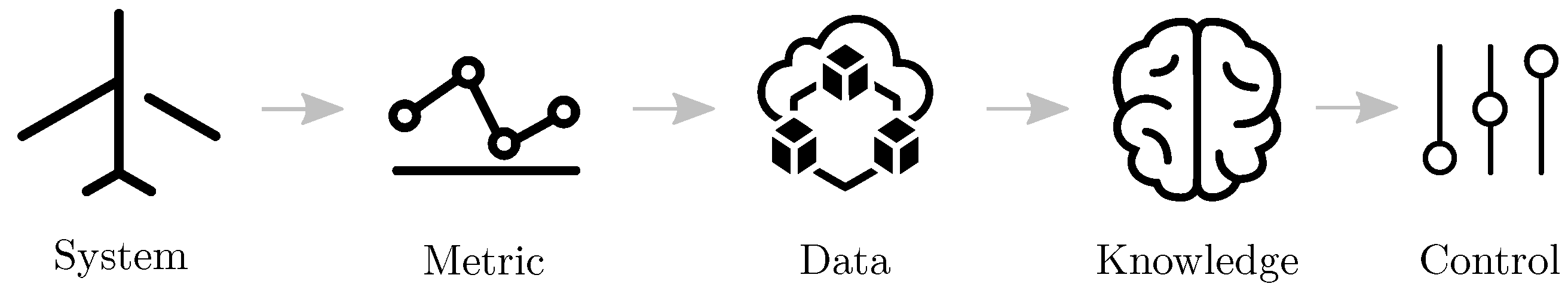
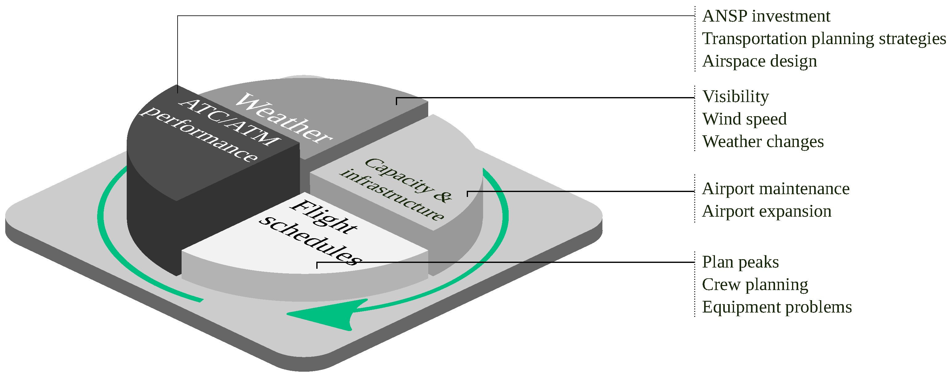
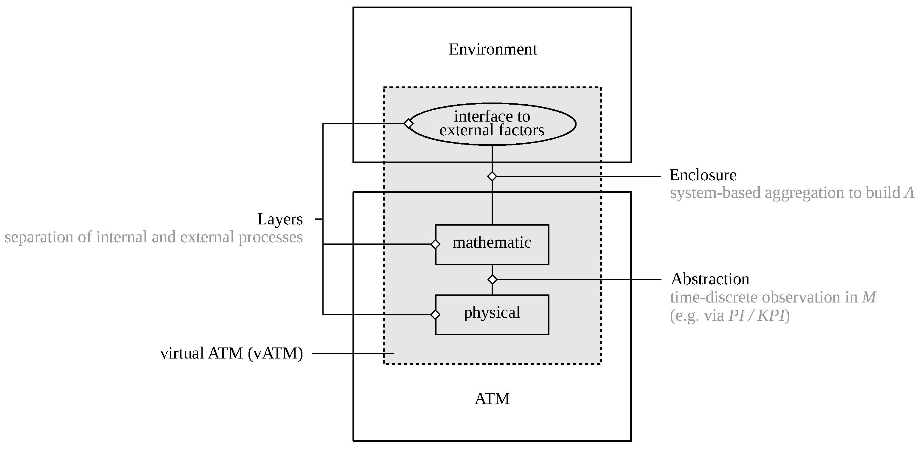
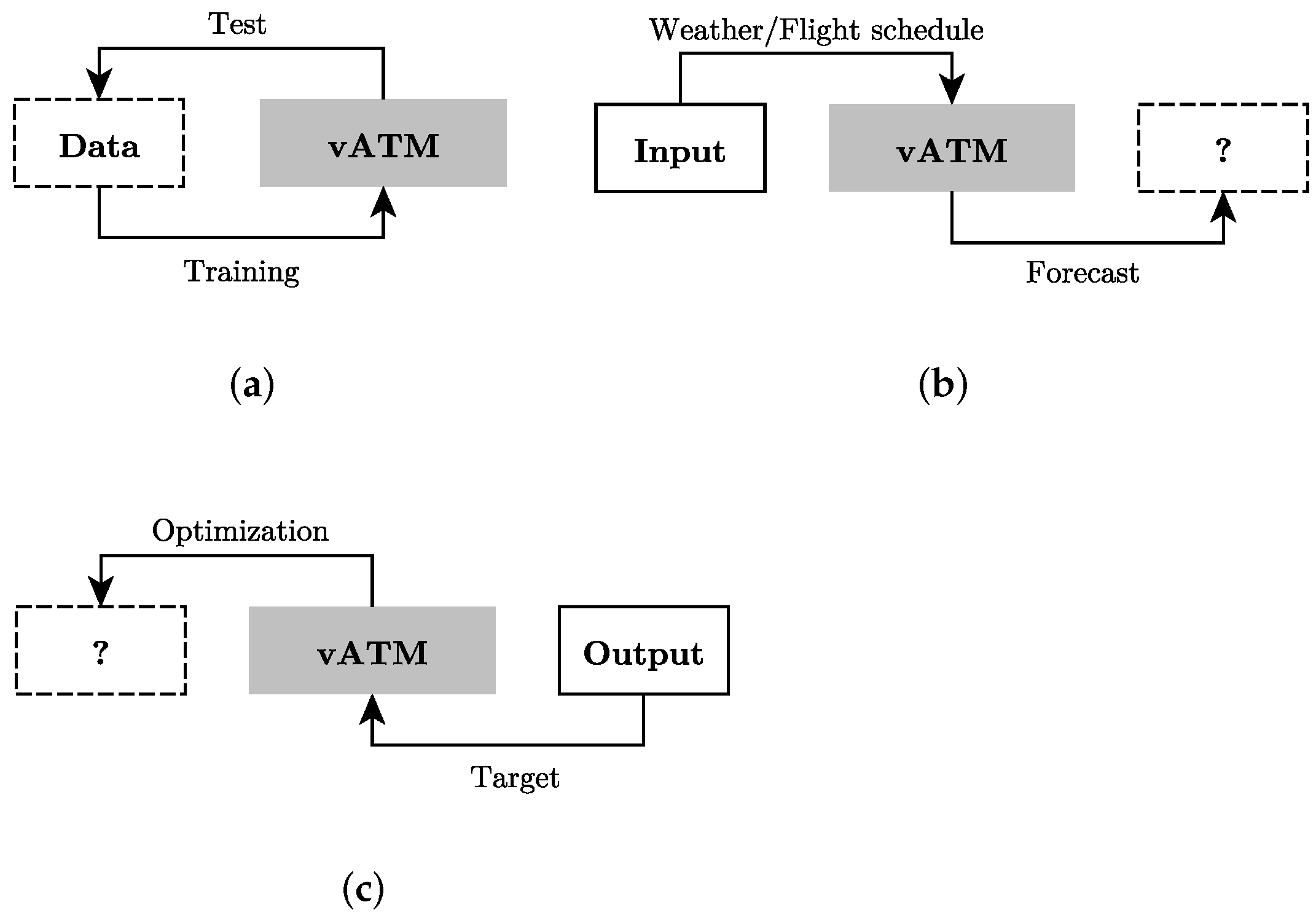
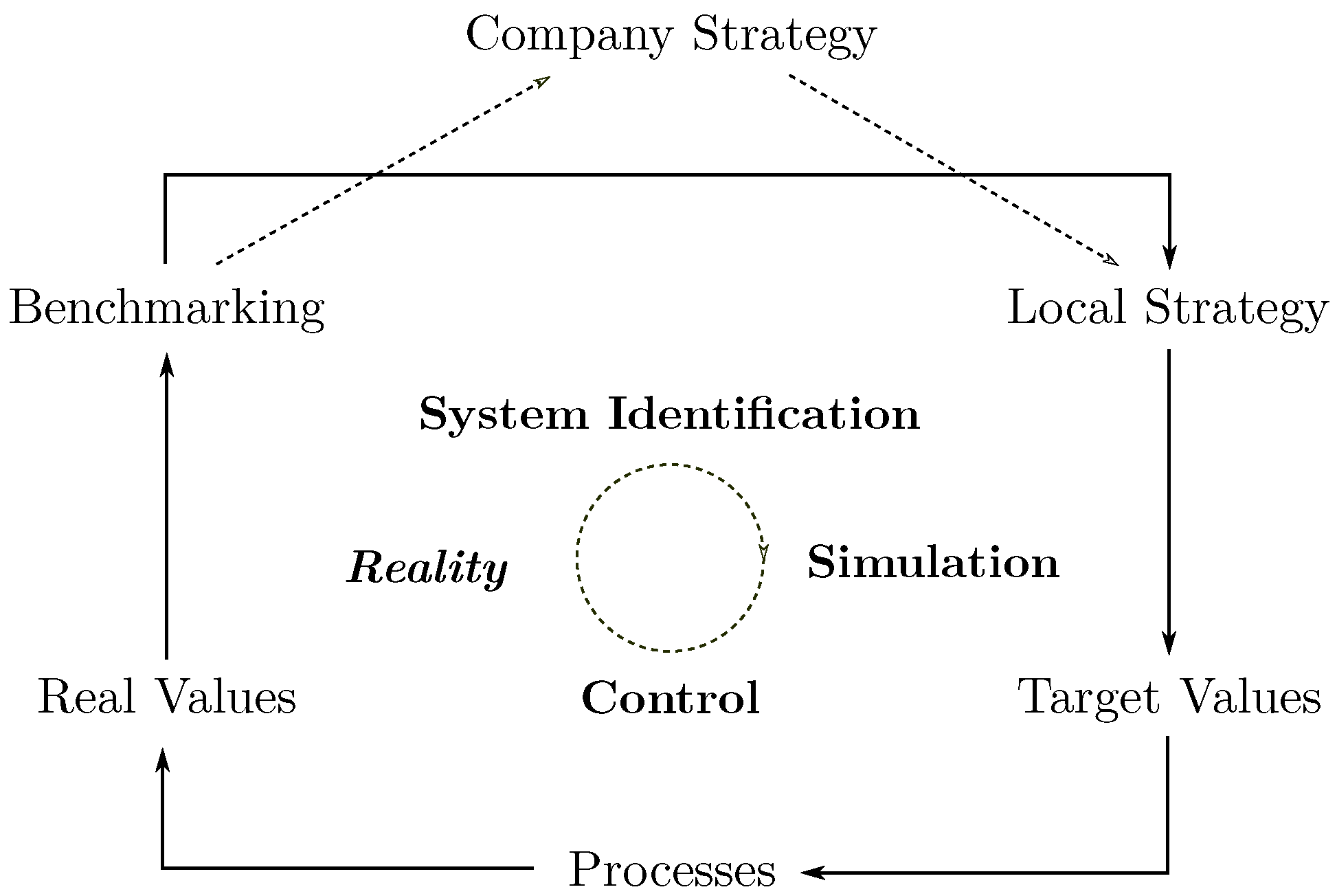
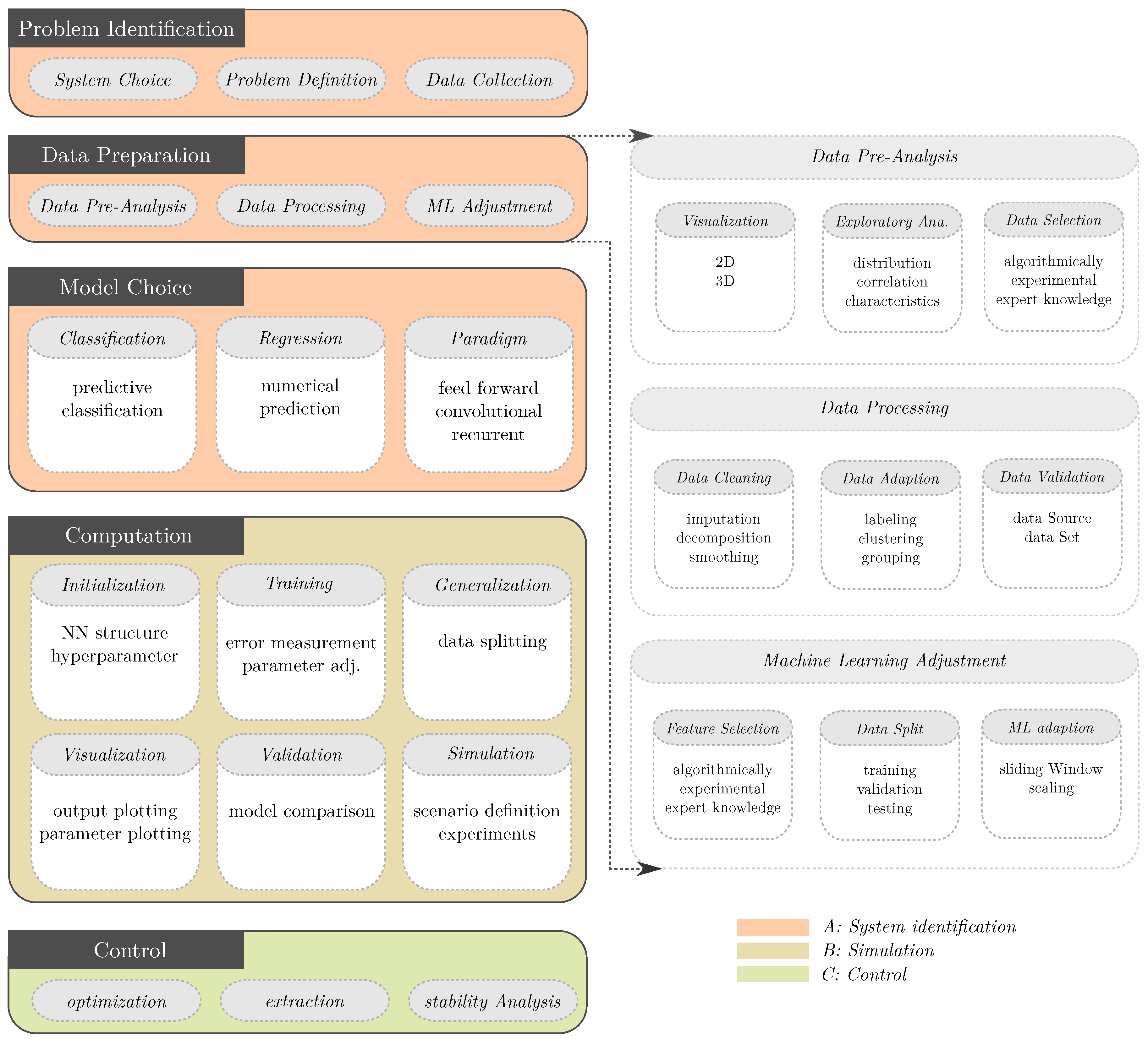
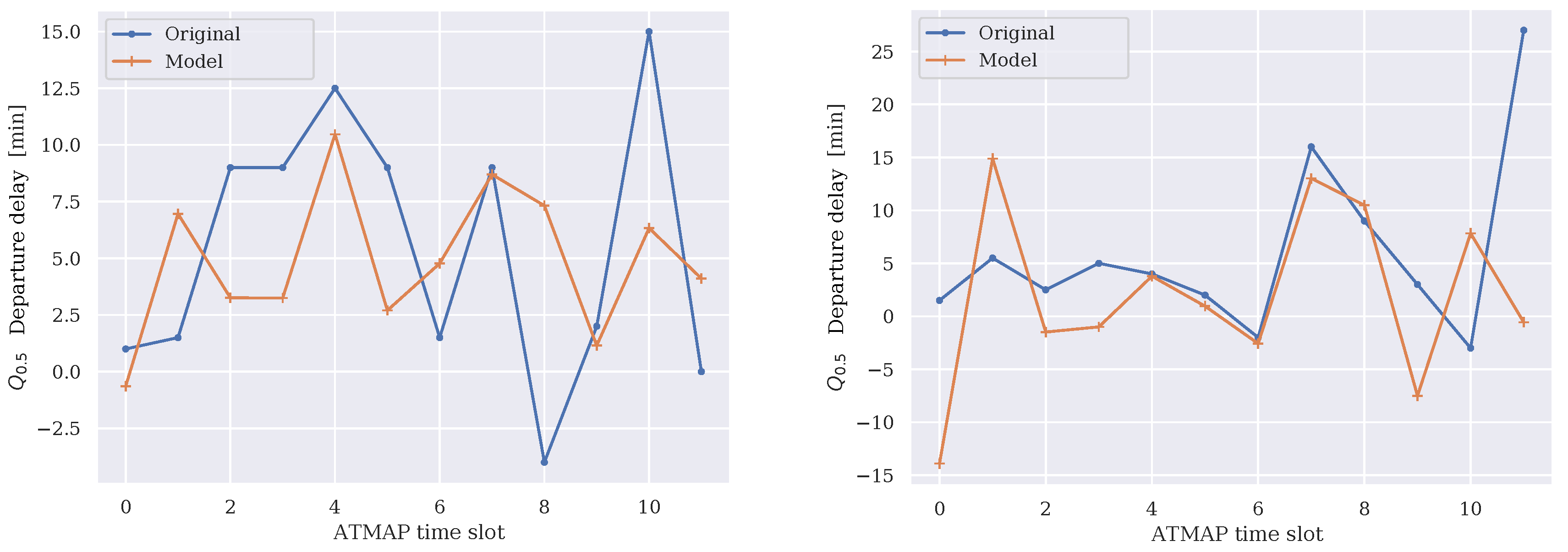
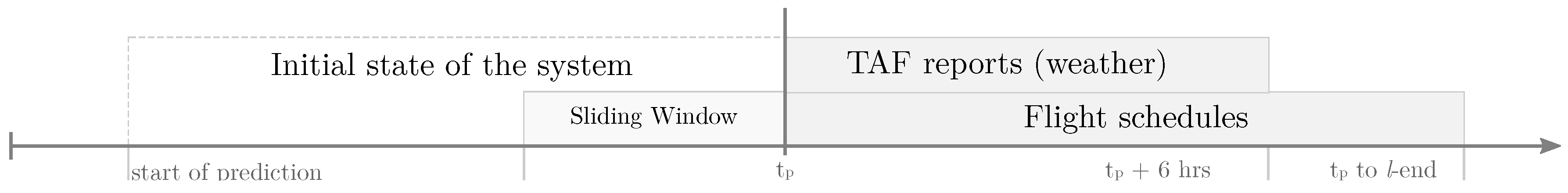
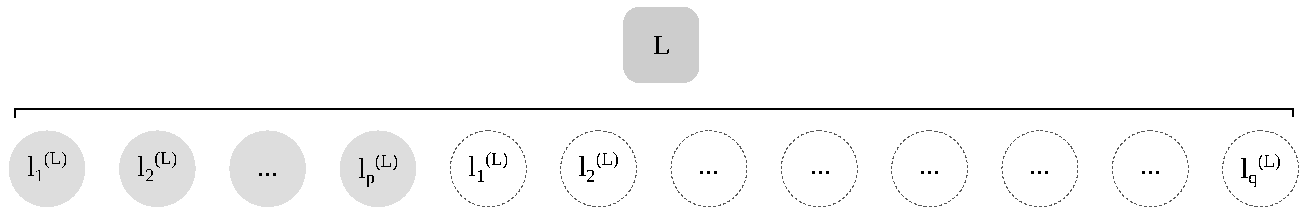
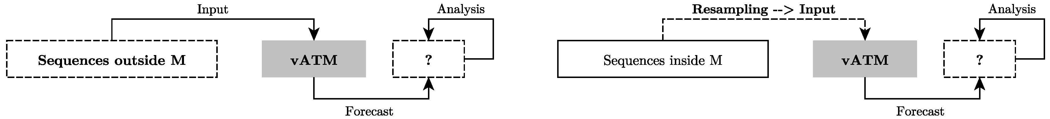
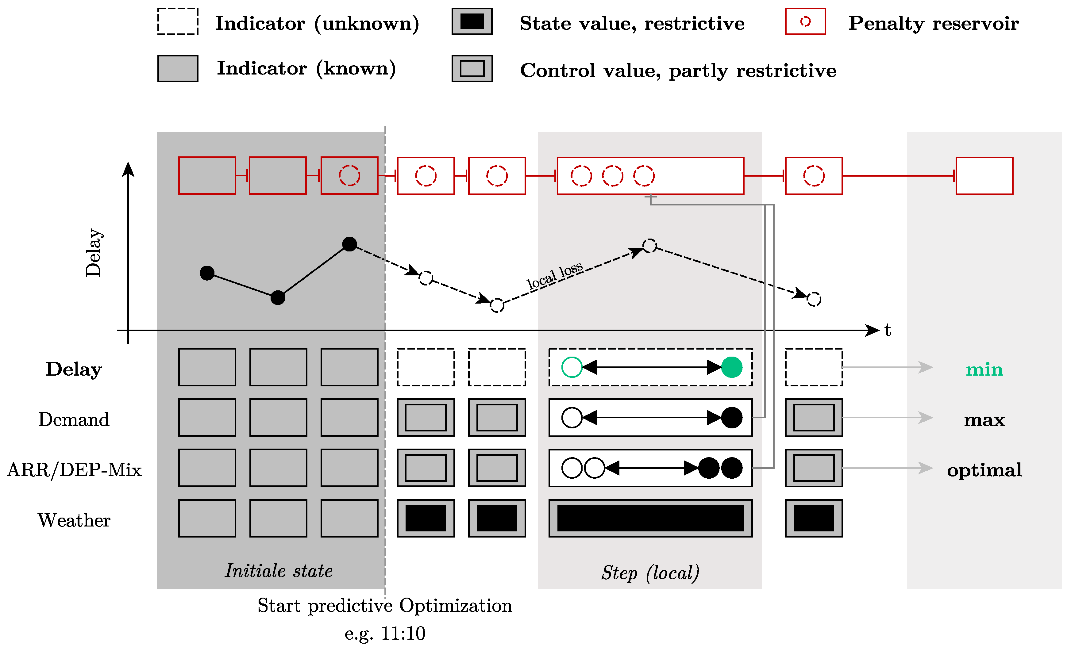
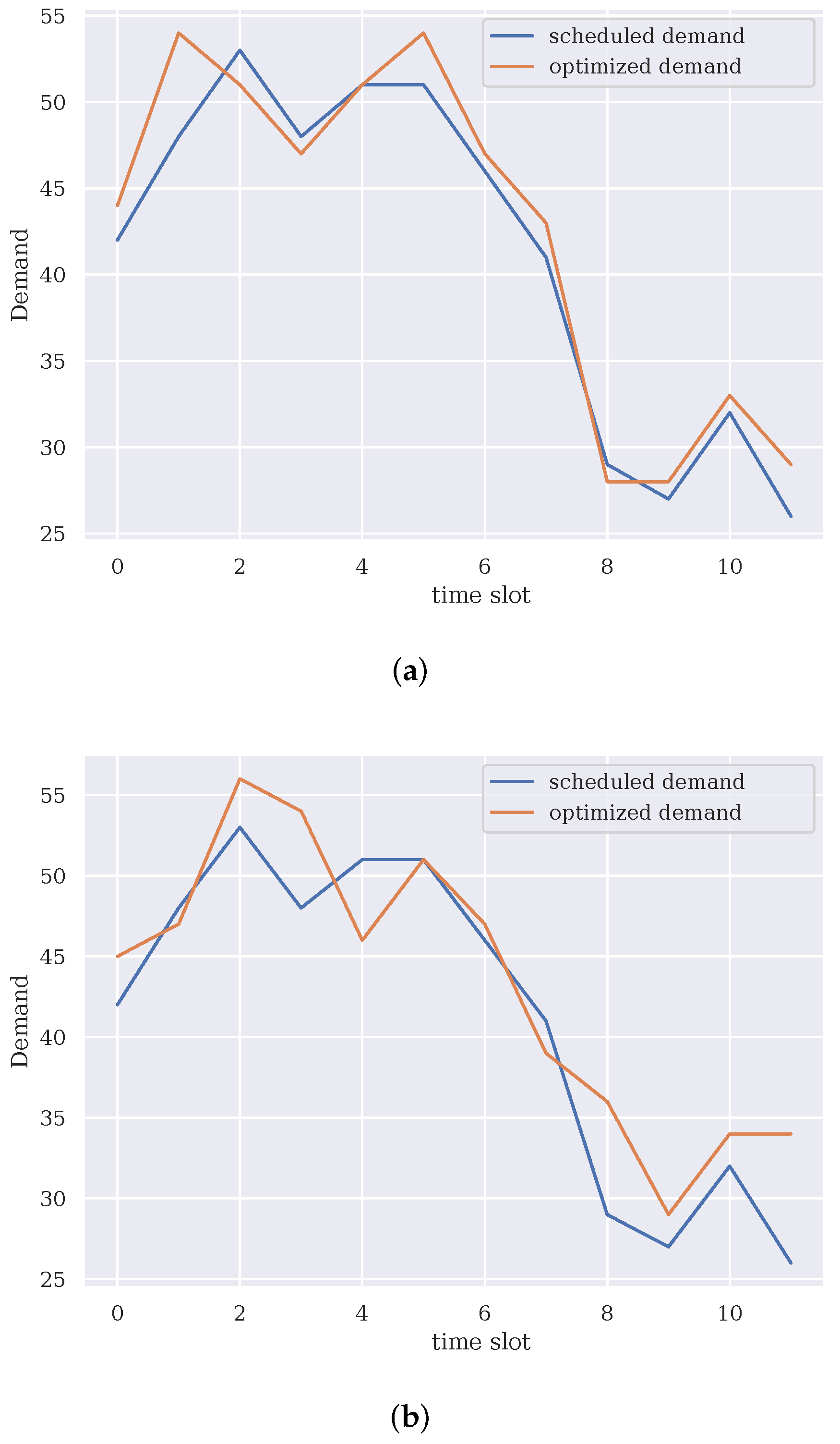
Table 1.
Summary of the used ANN with different uses cases at airports HAM and LGW, as well as boarding of an Airbus A320.
Table 1.
Summary of the used ANN with different uses cases at airports HAM and LGW, as well as boarding of an Airbus A320.
| A: Hamburg Airport (HAM) | B: Airport Gatwick Airport (LGW) | C: Boarding Airbus A320 | |
|---|---|---|---|
| Data source(s) | Flightstats, FlightRadar24, Openflights | simulation [30] | |
| Time domain | 2013 | 2012–08/2015 | 25.000 boardings for 6 strategies |
| Data tuples | 12.762 | 63.854 | 150.000 |
| Features | 9 | 12 | 4 |
| Goal of artificial neural networks (ANN) | prediction & classification of flight delays | prediction of boarding time | |
| Publication | [4,5,6] | [3] | |
Table 2.
Example data tuples for Hamburg Airport (HAM) to form L and l, 10.06.2013.
 |
Table 3.
The three core components system identification, control and simulation in the application of ANN.
Table 3.
The three core components system identification, control and simulation in the application of ANN.
| Input X | System | Output y | Description |
|---|---|---|---|
| given | unknown | given | System identification: ways to create a data-based virtual system map (vATM), taking into account process-related constraints (e.g., weather influence, flight demand). |
| given | given | unknown | Simulation: prediction of system state given known input quantities to estimate future behavior patterns (e.g., delay evolution). |
| unknown | given | given | Control: deriving recommended actions to achieve defined objectives (e.g., flight demand estimation to minimize delays). |
Table 4.
Framework modules for system identification (A), simulation (B) and control (C).
| Module | Description |
|---|---|
| A1: Problem identification | Detailed consideration of the purpose for which a system identification needs to be performed and how it will be used |
| A2: Data structure analysis | Includes modules to evaluate data base |
| Data pre-analysis | Exploratory analysis and visualization of data to select appropriate inputs |
| Data processing | Data adaptation to the ML problem, error analysis if necessary |
| Artificial neural networks (ANN) adjustment | preparation for application, selection of features and training data |
| A3: Model choice | |
| Regression | Direct mapping of discrete targets from multiple inputs |
| Classification | Reduction of correlation analyses to labels/intervals |
| Paradigm | Feed forward, recurrent, convolutional (depends on target) |
| A/B: Computation | Translation from learning (system identication) to forecast/prediction (simulation) |
| C: Control | Includes extraction, optimization and stability of the artificial neural networks (ANN) |
Table 5.
PSO results of calculations at LGW under reallocation of STA and STD at full demand satisfaction for example day 5 January 2015.
Table 5.
PSO results of calculations at LGW under reallocation of STA and STD at full demand satisfaction for example day 5 January 2015.
| Original | ∑ | Delay [min] | ||||||
|---|---|---|---|---|---|---|---|---|
| Demand | 48 | 48 | 51 | 41 | 27 | 26 | 494 | |
| STA | 21 | 25 | 23 | 16 | 13 | 21 | 252 | 13.44 |
| STD | 28 | 23 | 23 | 25 | 14 | 5 | 242 | |
| PSO | ∑ | Delay [min] | ||||||
| Demand | 54 | 47 | 54 | 43 | 28 | 29 | 509 | |
| STA | 23 | 24 | 29 | 17 | 12 | 22 | 254 | 12.09 |
| STD | 31 | 23 | 25 | 26 | 16 | 7 | 255 |
Publisher’s Note: MDPI stays neutral with regard to jurisdictional claims in published maps and institutional affiliations. |
© 2022 by the authors. Licensee MDPI, Basel, Switzerland. This article is an open access article distributed under the terms and conditions of the Creative Commons Attribution (CC BY) license (https://creativecommons.org/licenses/by/4.0/).
Share and Cite
MDPI and ACS Style
Reitmann, S.; Schultz, M. An Adaptive Framework for Optimization and Prediction of Air Traffic Management (Sub-)Systems with Machine Learning. Aerospace 2022, 9, 77. https://doi.org/10.3390/aerospace9020077
AMA Style
Reitmann S, Schultz M. An Adaptive Framework for Optimization and Prediction of Air Traffic Management (Sub-)Systems with Machine Learning. Aerospace. 2022; 9(2):77. https://doi.org/10.3390/aerospace9020077
Chicago/Turabian StyleReitmann, Stefan, and Michael Schultz. 2022. "An Adaptive Framework for Optimization and Prediction of Air Traffic Management (Sub-)Systems with Machine Learning" Aerospace 9, no. 2: 77. https://doi.org/10.3390/aerospace9020077
Note that from the first issue of 2016, this journal uses article numbers instead of page numbers. See further details here.