
Explanation of Machine-Learning Solutions in Air-Traffic Management


School of Engineering, RMIT University, Melbourne, VIC 3083, Australia
*
Author to whom correspondence should be addressed.
Aerospace 2021, 8(8), 224; https://doi.org/10.3390/aerospace8080224
Submission received: 3 June 2021
/
Revised: 13 July 2021
/
Accepted: 31 July 2021
/
Published: 12 August 2021
(This article belongs to the Collection Air Transportation—Operations and Management)
Abstract
:Advances in the trusted autonomy of air-traffic management (ATM) systems are currently being pursued to cope with the predicted growth in air-traffic densities in all classes of airspace. Highly automated ATM systems relying on artificial intelligence (AI) algorithms for anomaly detection, pattern identification, accurate inference, and optimal conflict resolution are technically feasible and demonstrably able to take on a wide variety of tasks currently accomplished by humans. However, the opaqueness and inexplicability of most intelligent algorithms restrict the usability of such technology. Consequently, AI-based ATM decision-support systems (DSS) are foreseen to integrate eXplainable AI (XAI) in order to increase interpretability and transparency of the system reasoning and, consequently, build the human operators’ trust in these systems. This research presents a viable solution to implement XAI in ATM DSS, providing explanations that can be appraised and analysed by the human air-traffic control operator (ATCO). The maturity of XAI approaches and their application in ATM operational risk prediction is investigated in this paper, which can support both existing ATM advisory services in uncontrolled airspace (Classes E and F) and also drive the inflation of avoidance volumes in emerging performance-driven autonomy concepts. In particular, aviation occurrences and meteorological databases are exploited to train a machine learning (ML)-based risk-prediction tool capable of real-time situation analysis and operational risk monitoring. The proposed approach is based on the XGBoost library, which is a gradient-boost decision tree algorithm for which post-hoc explanations are produced by SHapley Additive exPlanations (SHAP) and Local Interpretable Model-Agnostic Explanations (LIME). Results are presented and discussed, and considerations are made on the most promising strategies for evolving the human–machine interactions (HMI) to strengthen the mutual trust between ATCO and systems. The presented approach is not limited only to conventional applications but also suitable for UAS-traffic management (UTM) and other emerging applications.
1. Introduction
In traditional air-traffic management (ATM), artificial intelligence (AI) has been used to enhance air traffic and airspace operational efficiency for decades [1,2,3,4]. A significant contemporary challenge is the integration of the unmanned aircraft system (UAS) into both current and future ATM contexts [4], as the current ATM systems are unable to cope with the envisaged increase in air traffic densities, especially in low-level operations and in urban environments. Within the same unit of airspace volume considered, the magnitude of information that UAS-traffic mangement (UTM) needs to exchange, process, and track is much higher than that of conventional ATM. If not properly addressed, these conditions will compromise the safety of airspace operations whenever unforeseen perturbations introduce major deviations from the nominal flight plans [5]. Thus, computationally efficient optimisation algorithms are needed to deal with the increasing amounts of exchanged and processed data, constraints, and objectives characterising future ATM/UTM paradigms. In this context, future ATM and UTM decision-support systems (DSS) are expected to significantly rely on artificial intelligence (AI), which allows moving away from the limited flexibility of algorithmic logics typically found in declarative automation [4]. Increases in automation complexity and in the amount of processed information are eliciting further research in human–machine interactions (HMI) towards improving human–machine coordination and teaming [6]. ATM DSS have progressively evolved to enhance the support provided to the ATM operator’s decision-making process [7,8,9]. Since each task has unique objectives and constraints, the ATM system needs different types of analytics and reasoning techniques for different tasks. Nonetheless, utilising complex AI inference with characterised by a black-box behaviour could lead to a lack of transparency and a consequent loss of the operator’s trust and situation awareness. The black-box model only presents the final solution to the operator without showing the rationale behind [10], which challenges human ability to verify and understand the suggested solution. However, this verification is crucial, specifically for applications where systems need to be traceable for safety-critical operations [11]. Therefore, emerging ATM/UTM applications of AI is expected to elicit an evolution of design and certification methodologies to ensure the ongoing acceptance and trust by end-users. The research community is developing the optimal formats to present an explanation in a manner that the machine will be more likely trusted by human operator to the appropriate level, minimising both unwanted overtrust and distrust. State-of-the-art eXplainable AI (XAI) approaches are also being evaluated in terms of their support to integrated human-autonomy decision making, enhancing understandability and transparency [12]. However, the maturity of XAI algorithms and their presentation are currently limited in aerospace applications [13,14]. This paper focuses on the development of a viable solution to introduce XAI in the ATM DSS based on machine-learning (ML) inference.
With the current popularity of ML applications, various commonly used algorithms have been made available as open-source libraries. This allows researchers to rapidly integrate all the components from freely available libraries, thereby simplifying the prototyping of software and reducing barriers to access [15,16]. The paper reviews and investigates the most suitable and efficient open-source ML model that not only offers high prediction accuracy but also can be comprehended by the operator. The study investigates the feasibility and maturity of the proposed interpretable AI framework and focuses on the development of a ATM DSS functionality based on open-source algorithms and datasets. In particular, aviation occurrences and meteorological databases, which are both publicly available, are exploited to support the design of a hypothetical risk-prediction tool, which could support both present day ATM—as in the case of air-traffic advisory service in uncontrolled airspace—as well as future, performance-based autonomy concepts—for instance, by driving the inflation of avoidance volumes. The verification case study presented in this paper is restricted to conventional air-traffic data due to limited availability of UAS traffic data; however, the framework can be applied directly to UTM and urban air mobility (UAM) applications as soon as mature datasets become available.
The remaining parts of this section present a review of predictive models, XAI, and ATM HMI evolutions, whereas Section 2 introduces the theory underpinning the selected AI-prediction and explanation models. Section 3 describes the proposed implementation, datasets, model-training process, and performance metrics. The performance of the adopted AI inference engine is presented and discussed in Section 4. The explanation results and the proposed ATM HMI concept are presented in Section 5 and Section 6, respectively.
1.1. Predictive Methods
Traditional predictive methods are divided into two types: deductive methods based on governing theory (e.g., physics, mathematics) and inductive methods based on data analytics. Deductive methods strictly require the availability of theoretical models. Moreover, high degrees of realism and/or long forecast periods require high computing powers and/or time often beyond the available resources [17]. On the other hand, inductive methods include both statistical methods and ML methods. Statistical methods are derived strictly according to mathematical methods, meaning that the overall phenomenon is modelled by characterising the correlation between estimators and variables [18]. For instance, the time-series model, one of the most commonly used quantitative methods, only captures the patterns and temporal evolution based on the data without considering the causal structure of the occurrence [19]. As an example, Jaimyoung [20] proposed a linear regression model to predict the highway driving time from a few minutes to an hour in the future. These statistical models are mainly used for reasoning and estimation. Some assumptions and restrictions need to be introduced before model development, such as fixed algorithms and features that need to be manually identified and extracted.
Contrastingly, the structure of the ML algorithm is flexible, as it needs to assume that the input data can be very limited. Hence, it is very suitable to deal with complex and highly nonlinear relationships [21]. Ensemble learning is one of the most popular and promising ML algorithms. Its fusion methods include boosting, bagging, and stacking [22]. Ensemble learning not only explains the interaction between input variables and predictive models but also identifies the relative importance of the key factors. Gradient-Boosted Decision Tree (GBDT) is an integrated learning method based on the Decision Tree (DT). Unlike a traditional DT, the advanced modification enables GBDT to iteratively train a series of weak learners and strategically generate the best tree set to improve prediction accuracy [23]. Ramon [24] adopted the GBDT model to predict the take-off time, which provided more accurate prediction results than the Enhanced Tactical Flow Management System (ETFMS). The open-source model XGBoost, developed based on the GBDT framework, is adopted in this paper. This library has many advantages in processing nonlinear data and can extract features from variables containing noise and redundant information [25]. As an example, Gu et al. [26] proposed a lane-changing decision system for autonomous vehicles based on the XGBoost model. By making full use of large-scale dataset training, the XGBoost model has much better performance and practicability than conventional lane-changing systems. Global analysis of the features’ importance can explain the results of the XGBoost model to a certain extent.
1.2. Explainable AI (XAI)
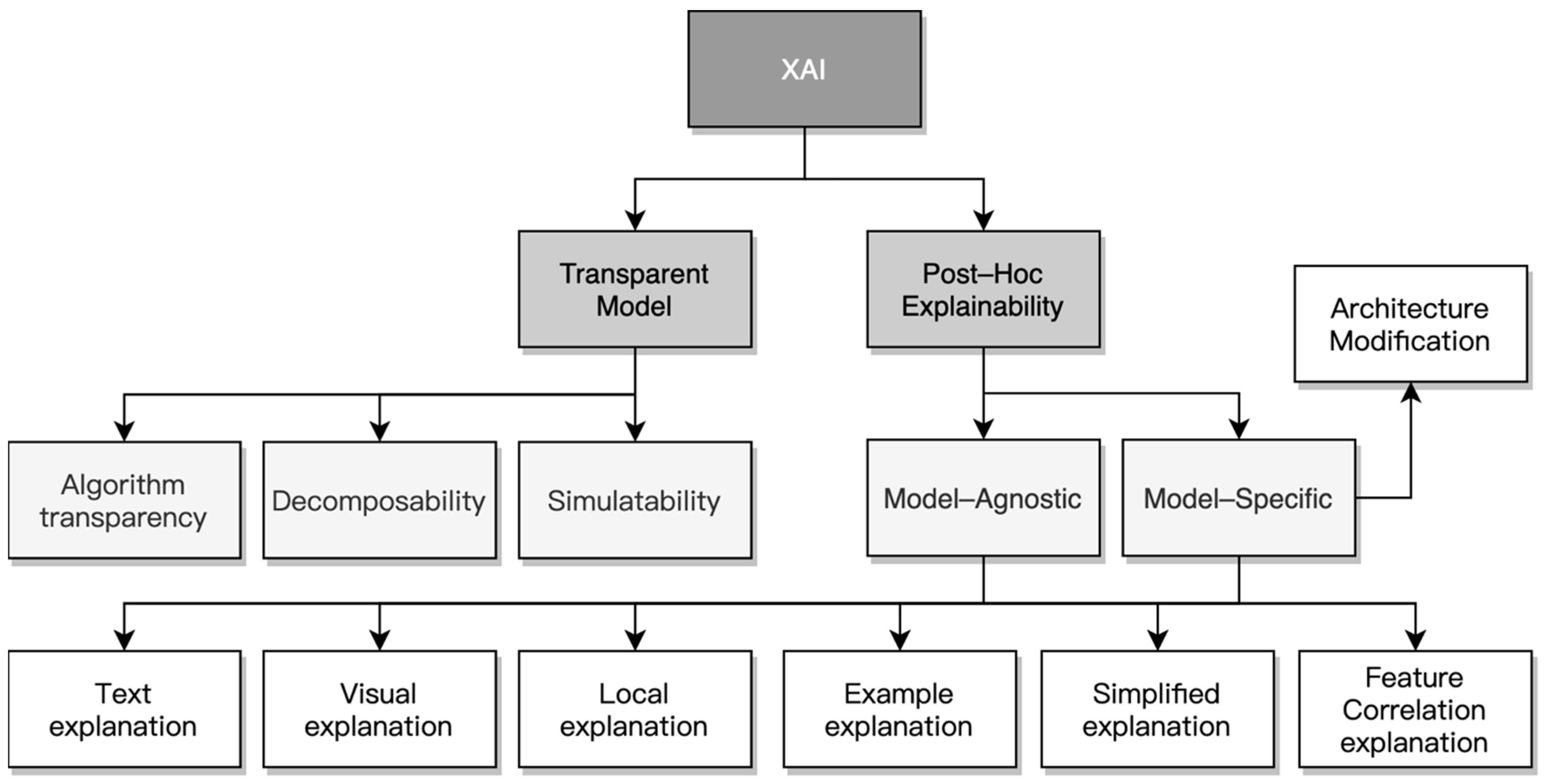
Most ML models lack the explainability of the algorithm itself and the output results, which then challenges the operator to understand and accept such a solution. Henceforth, post-hoc explanations models are considered in this research to enhance the explainability of the results. According to Arrieta et al. [13], the XAI method is systematically analysed, and its importance is divided into two-step classification, as shown in Figure 1.
The first classification is between interpretable models and post-hoc explainability XAI approaches and is based on the distinction between models that are inherently transparent and models for which a post-hoc explaination can be constructed. In particular, when the ML model does not inherently offer a transparent explanation, a particular method is needed to explain its decision so an additional classification can be encountered. Model-agnostic post-hoc explanation methods can be applied to any ML models, whereas model-specific methods are developed only for a specific ML model and will not work in conjunction with other techniques. Generally, black-box AI models will require a post-hoc explanation method. There are two types of explanation: global and local. The local explanation divides the complex model into simple individuals while also analysing the individuals’ relationship. The global explanation offers an overall understanding of the model, aiming to make the entire decision-making process completely transparent and comprehensive. Usually, it is necessary to utilise these two explanation methods simultaneously to satisfactorily explain the ML algorithm, which can effectively reduce the potential skew and uncertainty affecting a single method.
Due to the opacity of the black-box model, the post-hoc explanation model is used to interpret the prediction model and its results. However, a single explanation method limits and biases the interpretation and understanding of the black-box model. Therefore, two different explanation models are used to simultaneously explain a black-box algorithm and prediction results, thereby enhancing the interpretability of XGBoost incident and accident prediction. The mature and freely available post-hoc explanation models considered in this study are SHapley Additive exPlanations (SHAP) and Local Interpretable Model-Agnostic Explanations (LIME). SHAP is a visual local explanation method for tree models. While assigning the weight and value to each feature, the local explanation is extended to capture the features’ interaction directly, and a large number of local explanations are used to understand the global structure. Besides, its built-in visual components can intuitively display the influence of complex variables [27]. The LIME model, on the other hand, is completely independent from the prediction model itself and only attempts to explain its results. In other words, LIME can explain any black-box prediction without inspecting the model. These two XAI methods are supported by XGBoost that aims to further explain the prediction results in more detail and highlight the driven factors of the results.
1.3. Human–Machine Interactions
Current developments of the ATM system and interface technology are aimed at accommodating denser traffic. A number of HMI innovations have been proposed for ATM implementation supported by system evolutions [28]. The two common design streams are visualisation [29,30,31] and control function improvements in DSS [7,8,9]. With the increasing AI exploitation in decision-support tools, the air-traffic controller (ATCo)/air-traffic control operator (ATCO)’s concerns when working with highly automated systems have not diminished but instead have been exacerbated [32]. Experienced human operators tend to be reluctant to adopt suggested solutions from highly autonomous DSS if these are not trustworthy, traceable, and interpretable, especially in very complex situations [14]. Hence, DSS are required to adopt XAI to increase the understandability and trust of human operators. One emerging concept that aims to enhance the cognitive states of the human operator in real time during the complex and time-critical operations with a high level of automation is Cognitive Human–Machine Interfaces and Interactions (CHMI2) [33,34]. A human cognitive state monitoring/enhancement by machine prevents cognitive overload and human oversight when increasing the level of autonomy in decision-support systems. The CHMI2 framework is comprised of three main modules: sensing, inference, and adaptation. Similar to other proposed HMI concepts in the literature, the CHMI2 sensing module also uses advanced neurophysiological sensors, which are, however, used to collect the responses in real time. The collected and pre-filtered data are passed through the inference module to estimate the cognitive state of the operator. This inferred cognitive state is the key driver to dynamically adapt the HMI formats/functions and automation behaviour [35].
2. Prediction and Explanation Models
This section introduces the theory underpinning the predictive AI algorithm adopted in this study and subsequently the post-hoc explanation methods that were implemented. The first part introduces the rationale and equations of the XGBoost predictive model to describe its operating principle. The second part explains the operating principles and equations of two different interpretation models, which are LIME and SHAP.
2.1. XGBoost
XGBoost is a library developed from the GBDT algorithm to combine multiple weak learners through the boosting method [36]. The basic algorithm is based on the Classification And Regression Trees (CART), which has high performance in both interpretability and transparency [37]. XGBoost has seven main hyper-parameters that can be adjusted to improve the algorithm’s progress and robustness and also to reduce overfitting. The set of hyperparameters include:
- Learning rate: in order to prevent overfitting, a shrink step is used in the update process. Each time the weight of a leaf node is updated, the learning-rate coefficient is multiplied to avoid excessive step sizes. A small learning rate can improve the robustness of the model;
- Maximum depth: this value is the maximum depth of branching of the tree, which is also used to avoid overfitting. The larger the value, the easier it is for the model to learn more specific and local samples;
- Minimum child weight: this parameter represents the minimum sample weight required to generate a child node. When the sum of the weights of all samples on the leaf node is less than the set value, the construction process will stop splitting. This parameter is used to avoid over-fitting. When the value is large, it can prevent the model from learning local anomalies in the training data;
- Maximum number of iterations: this is the maximum number of trees generated and also the maximum number of iterations. The higher the number of trees, the better the performance, and more computing time is required;
- Lambda regularisation: this is used to control L2 regularity. It is the coefficient in front of the score of the leaf node in the objective function;
- Alpha regularisation: This is used to control L1 regularity. It also speeds up the algorithms in very high dimensions;
- Gamma value: in order to further split the leaf nodes of the tree, the minimum loss reduction must be set. In other words, the split is determined by observing whether the loss has decreased;
- Sub-sample: this parameter controls the proportion of random sampling for each tree; too large or too small a value will lead to over-fitting and under-fitting of the model.
Equation (1) illustrates the basic CART formula, where is the number of trees, represents all possible CART trees, and represents a specific CART tree.
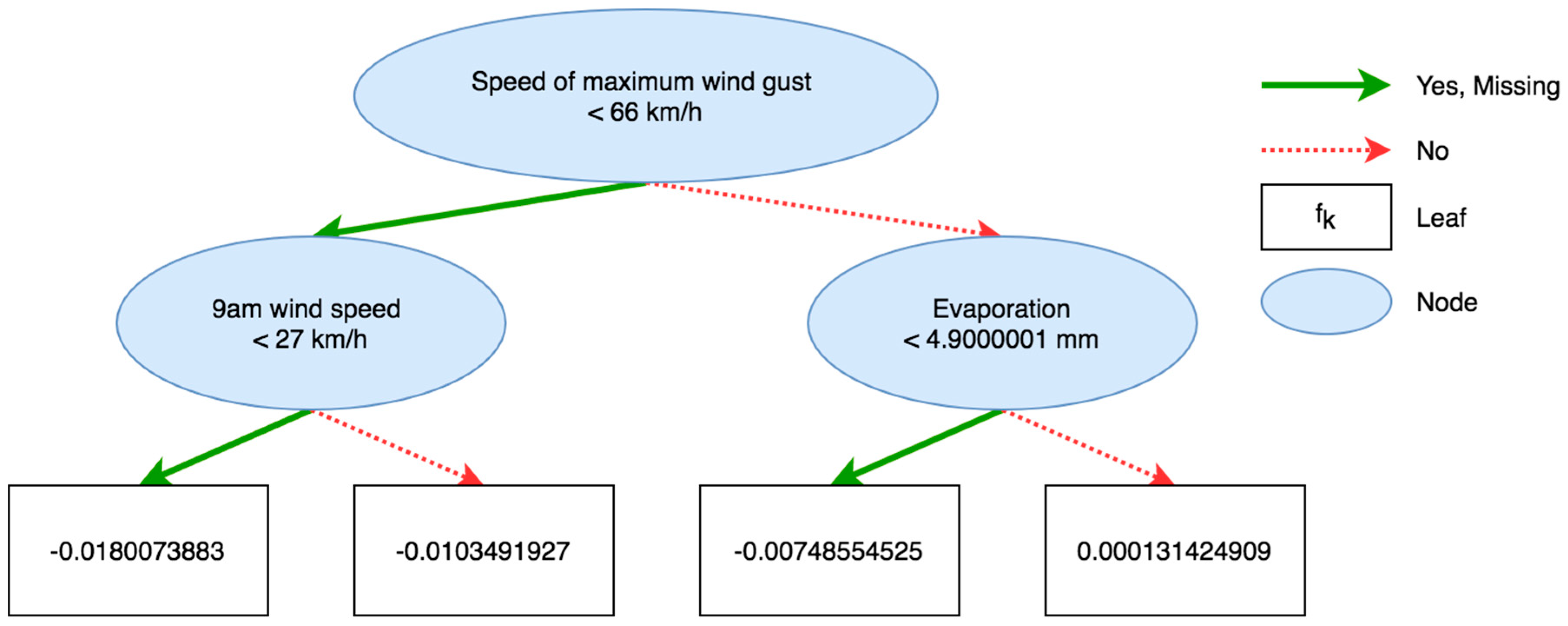
The training of the model is essentially additive training. Figure 2 illustrates an example of a CART prediction model. The algorithm also classifies the missing values of each node. The number in the leaf is the value of . The detailed mathematical formulation of the XGboost algortithm is presented in Appendix A.
2.2. Post-Hoc Explanation Model
The global explanations of prediction results from XGBoost can be enhanced by adopting two post-hoc local explanation models: SHAP and LIME. These two models are supported by XGBoost with the aim of explaining the prediction results in more detail and highlighting the factors driving the results. Table 1 summarises the differences between LIME and SHAP.
2.2.1. LIME
The LIME method is used to explain the prediction of any classifier or regression model [38]. It does not interface with the algorithm inside the black box but randomly generates input data to collect aggregate outputs. The feature importance is obtained by comparing the prediction results between the artificially perturbed data and original example, thereby generating an explanation for each single prediction of any ML models. Out of the various possible explanations, LIME selects the explanation to be presented to the human operator based on the following minimisation problem [38]:
where represents the black-box model that needs to be explained; and are, respectively, the explanation model and the collection of potentially interpretable models; is the distance between data in the new dataset and the original data instance; L defines the model fidelity, which is a measure of how unfaithful the explanation is in approximating the original model around is the complexity of the model, which shall be low enough to be interpretable by the human operator.
2.2.2. SHAP
SHAP is an alternative method for local ML explanation. It is a method based on the concept of game theory to calculate the importance of additive features for each specific prediction [39]. Similar to the feature correlation explanation, the method describes the function of the opaque model by ranking or measuring the impact, relevance, or importance of each feature in the prediction output. Lundberg et al. [27] developed TreeExplainer based on SHAP, which is a visual local explanation method. While assigning the weight and value of each feature, the local explanation is extended to capture the interaction of the features directly, and a large number of local explanations are used to understand the global structure. It calculates the Shapley value or attribution value of each feature and then measures the impact of the feature on the final output value [40,41]:
where represents the explanation model; is the number of input features; represents whether the feature exists; and is the attribution value of each feature (Shapley value).
The output of the decision tree conditioned on the feature subset is defined as . The SHAP value is based on game theory to average all possible conditional expectations. For a certain feature , it is necessary to calculate the Shapley value for all possible feature combinations (including different orders) and then weighted summation:
where is a subset of the features used in the model; is the vector of feature values of the sample to be explained; and is the number of features.
The working principle is to average the marginal contribution of all sequences. In other words, by entering all the sequences, the marginal revenue generated by each feature is obtained, and then all the gains are averaged, and finally, the Shapley value is calculated for each feature.
The SHAP methodology supports various types of explanation plots. In this paper, two plots are chosen to analyse and explain the results of model predictions: summary plot and dependence plot. The models fulfil the gap that other models cannot provide, which is to present how each feature matters and its effect distribution. It is vital for operator decision making when further reasoning is required. The summary plot shows the potential interactions between various features, allowing the global features to be interpreted through this local explanation. The dependence plot also explains the contribution of a single variable to the predicted value and analyses individual features in more detail.
3. Model Implementation and Verification Methodology
This section describes the AI explanation model implementation as well as the verification methodology. The first part explains the overall framework of prediction and explanation model integration followed by dataset selection and data preparation. Lastly, the performance metrics are discussed for model performance evaluation.
3.1. Prediction Framework
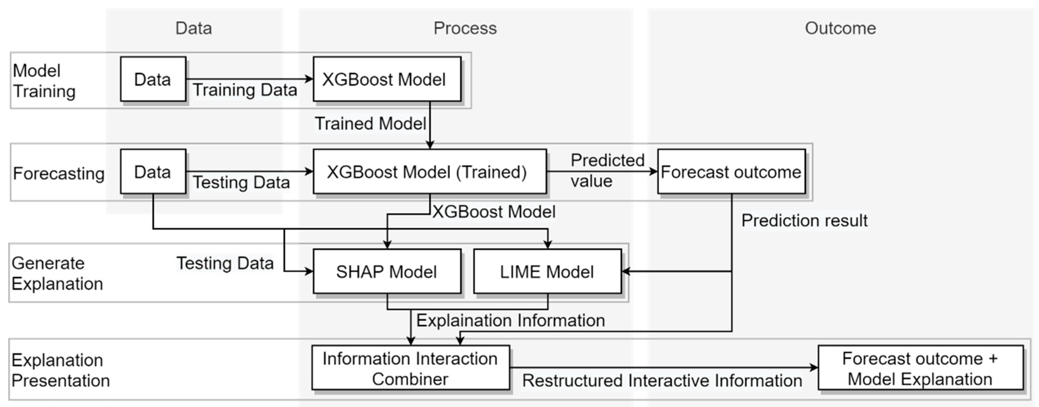
The implemented prediction framework is illustrated in Figure 3. In the initial stage, a trained XGBoost model is generated by inputting labelled training data. Successively, testing data are fed into the trained model to obtain representative prediction results. The accuracy of the prediction model is assessed by comparing the prediction results with actual labelled values. The system integrates the SHAP model and the LIME model to obtain two post-hoc explanations. The SHAP model requires testing data and the trained model, while the LIME model requires the input of testing data and forecast results. These models provide the explanation of the trained model and the explanation of the specific parameters. Finally, the two explanation modes and forecast results are integrated and displayed through the interaction module. In the verification case study presented in the following section, the XGBoost library is trained to predict the risk of incidents and accidents based on meteorological data, which allows to implement a real-time situation-assessment tool for air-traffic advisory services of the kind provided in present day ICAO airspace Classes D, E, and F. The same risk-assessment functionality can also be exploited to drive the inflation of avoidance volumes in emerging performance-based ATM/UTM concepts involving autonomous separation assurance and collision-avoidance services.
The adopted development environment to implement and test the prediction model is Python 3.7.8, with four computing libraries, which are Numpy 1.18.5, Pandas 1.0.5, Scikit-learn 0.23.1, XGBoost 1.3.0., LIME 0.2.0.1, and SHAP 0.36.0. NumPy (Numerical Python) is an extended library of the Python language. In this particular activity, the main function is to process the N-dimensional array generated when inputting data and handle abnormal values. Pandas is a tool based on Numpy, which mainly solves input data analysis and exploration tasks. Usually, NumPy and Pandas are used together. Scikit-learn and XGBoost are Python ML models. In this research, XGBoost mainly provides core algorithms, while Scikit-learn mainly provides pre-processing of input data and data analysis of output results.
3.2. Datasets
In this case study, due to the limited availability of publicly available traffic datasets, open-source databases of meteorological and aviation incidents and accidents have been adopted in the verification case study are collected from the Bureau of Meteorology [42] and ATSB (Australian Transport Safety Bureau) national aviation occurrence database [43]. The collected data are separated into two periods from 1 April 2018 to 31 March 2019 and from 1 July 2019 to 30 November 2019. The data location is in a 15 km radius of Melbourne Airport (latitude: 37.67 S, longitude: 144.83 E). The meteorological data comes from the Melbourne Airport site, numbered 086282. The data consist of daily comprehensive data: observation data at 9 a.m. and 3 p.m. The entire dataset is divided into five channels, as follows:
- ID and date
- Synthetic daily data
- Observation data at 9 a.m.
- Observation data at 3 p.m.
- Incidents and accidents report
To display the data and feature labels effectively, the feature names are simplified; for the operation of the model, the data of wind direction is converted from characters to numerical values; the incidents and accidents numerical value is translated into 0 and 1, corresponding to False and True, respectively. Table 2a details the full names corresponding to the abbreviations. Table 2b the codes corresponding to the wind-direction characters.
3.3. Model Preparation
The segmentation of the dataset is critical for the prediction model. The ratio of the train-test split directly affects the entire prediction model. If the testing set’s size is too small or too large, it causes insufficient model accuracy or lack of generalisation ability. If the training set is too large, this increases the risk of overfitting. The conventional data-split strategy in many research activities is a ratio of 80% training to 20% testing. In this research, the split ratio is 67% to 33%: two-thirds of the training set and one-third of the testing set. The purpose is to ensure that the model has enough data for training while reducing overfitting and increasing its generalisation ability. The total input data is 518 days, and the system randomly selects 347 days of data as the training set and 171 days of data as the test set. To obtain a better prediction accuracy, the test sets up three hyperparameters to compare the results: learning rate, maximum depth, and minimum child weight. The main purpose of these three hyperparameters is to prevent overfitting but in different ways:
- The learning rate helps to adjust the iteration step size, improving the model’s overall robustness by reducing the weight of each step;
- The maximum depth adjusts the number of specific samples and local samples that the model can obtain to avoid overfitting;
- The minimum child weight determines the sum of the minimum leaf node sample weights, thereby preventing the model from learning local special samples.
The learning rate ranges from 0 to 1. For the test, 1, 0.1, 0.01, and 0.001 were taken. The maximum depth range is from 0 to unlimited. In the test, 3, 5, 8, and 10 were taken. For minimum child weight, it will lead to insufficient fitting if the value is too high. Therefore, four values were chosen in the test, which are 1, 3, 4, and 7. The remaining hyperparameters are set to be fixed values, and no adjustments were made in this experiment, as shown below:
- Maximum number of iterations: 800
- Lambda regularization: 1
- Alpha regularization: 0.85
- Gamma value: 0.2
- Sub-sample: 0.85
The hyperparameter adjustment process has two main objectives. The first purpose is to optimise the Xgboost algorithm performance for the particular problem at hand, typically by adjusting the hyperparameters to maximise prediction accuracy. The other objective is to evaluate the influence of different hyperparameters on the prediction results. Some problems have good prediction results under certain hyperparameter settings, but once the hyperparameter settings are changed, the accuracy of the prediction results drops sharply. Therefore, by comparing the prediction results under different hyperparameter settings, it is possible to improve the versatility and usability of the system.
3.4. Performance Metrics
In regression problems, performance metrics like Mean Absolute Error (MAE), Root Mean Squared Error (RMSE), and Coefficient of Determination (R2) are commonly adopted. In this study, the accuracy of the predicting model is calculated based on Equation (5), where means the sum of the differences between each predicted value and its corresponding actual value. is the total number of test sets.
Area under the curve (AUC) is a binary model evaluation index that refers to the area under the receiver operating characteristic (ROC) curve. Equation (6) is the calculation of AUC.
In Equation (6), is the sum of all positive sample numbers, is the serial number of the sample , and and are the number of positive samples and the number of negative samples, respectively.
4. Model Performance Evaluation
The prediction performance of XGBoost is analysed by comparing the results from different hyperparameter combinations, as detailed in Section 3.3. Simultaneously, without resorting to other explanation methods, XGboost explains globally the trained model through its feature correlation analysis and feature importance analysis.
4.1. Prediction Outcomes
The accuracy of all models exceeds 85%, and the highest accuracy is 92.40% where the learning rate is 0.001, and minimum child weight is 7. Besides, the lowest accuracy is 86.55% when the learning rate is 1, the maximum depth is 5, and the minimum child weight is 1 and 3. The correct classification rate is high. AUC (area under the curve) is used to measure the robustness of the estimated model against overfitting. In the test, the lowest AUC value is 0.69 when the learning rate, minimum child weight, and maximum depth are 1, 1, and 3, respectively. Additionally, the highest values are 0.82 when the learning rate and minimum child weight are 0.1 and 5 and the maximum depth is 3, which shows that the prediction model has high robustness and high accuracy. Regardless of the hyperparameter setting, reliable accuracy and good robustness are obtained as a result. Therefore, the hyperparameters used in the training model are a learning rate of 0.001, minimum child weight of 7, and maximum depth of 3. All detailed test results of the XGBoost model trained according to different hyperparameters are shown in the Supplementary Data.
4.2. XGBoost Global Explanation
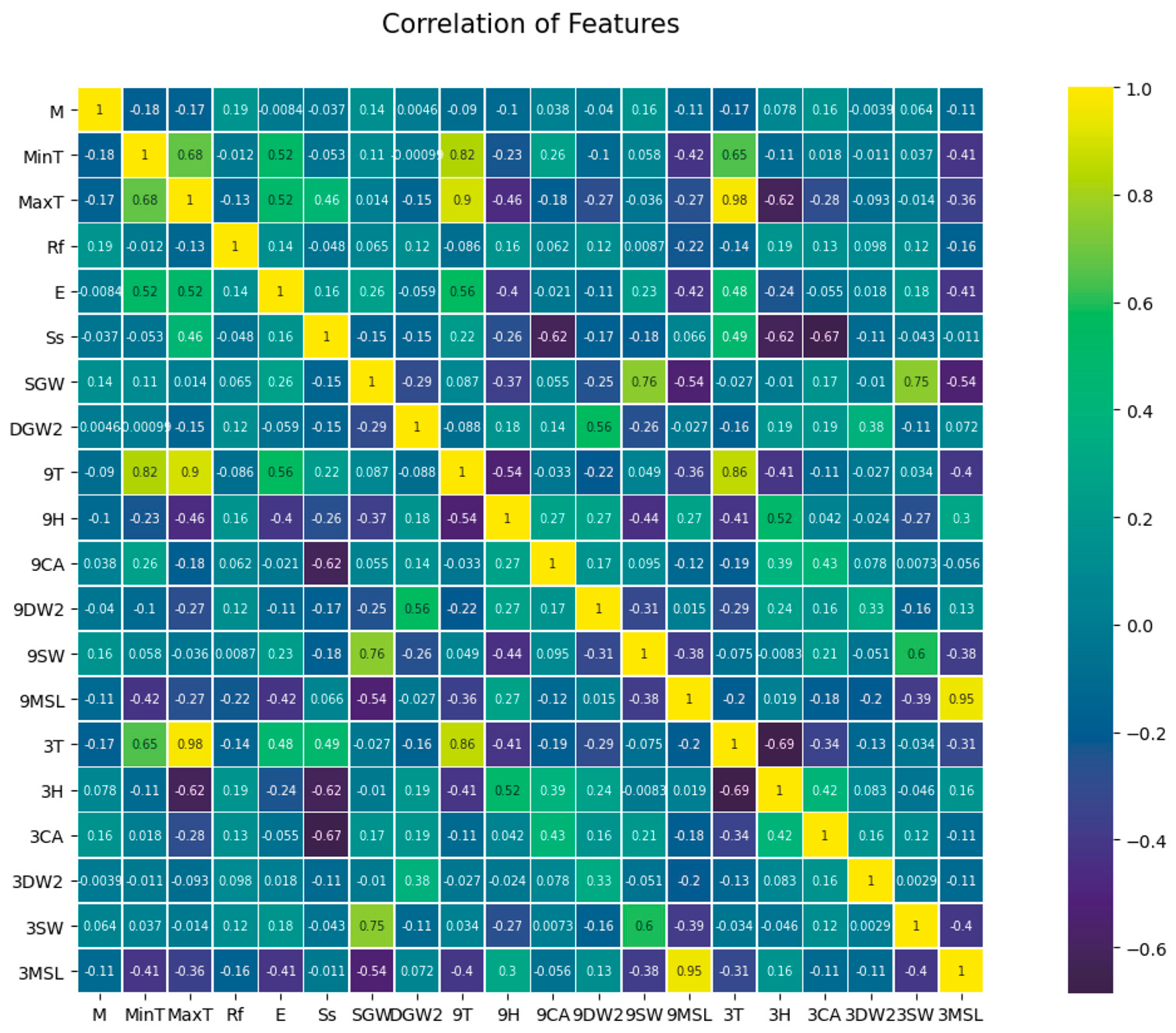
To be able to comprehend the model, the analysis of data features is crucial. The correlation between variables (features) in the input data can be observed in Figure 4. The highest positive correlation between two variables is 0.98, while the highest negative is −0.69. Temperatures in each period and MSL pressure are the most relevant features in the study. Remaining features have no close correlation among themselves.
XGBoost produces its inferences based on a tree model different from linear models; tree models are naturally robust to related variables [44]. For XGBoost, the existence of relevant variables will only increase the calculation time, but it will not significantly impact the accuracy of the model. When preparing the data in this experiment, the relevant variables were not screened because there were less than 20 types of variables.
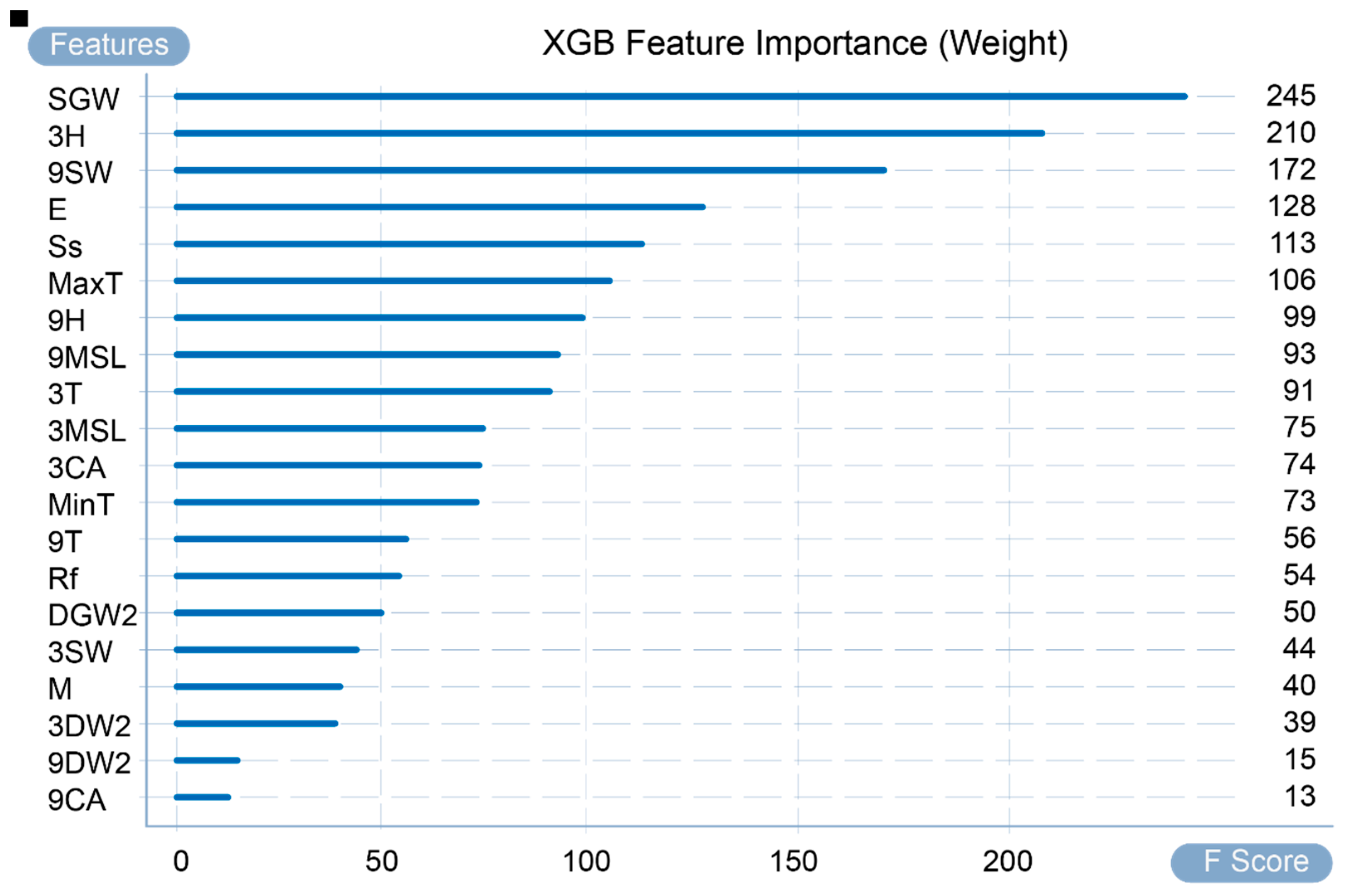
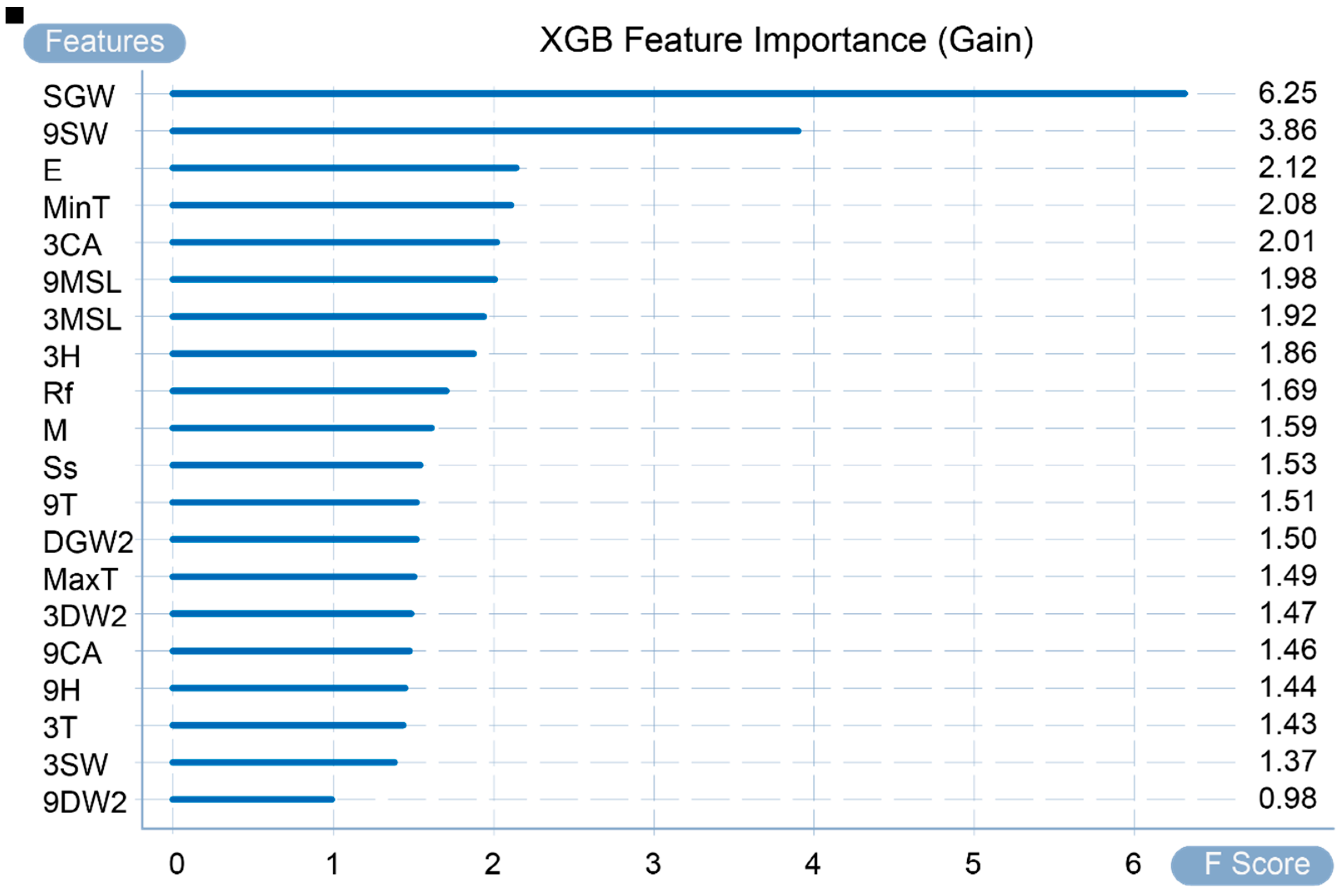
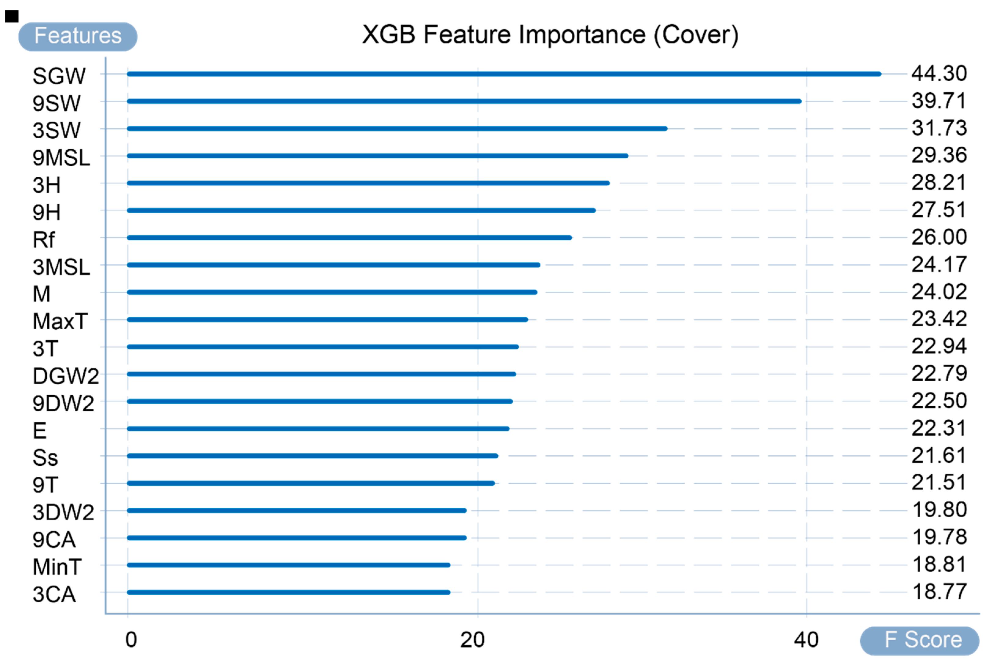
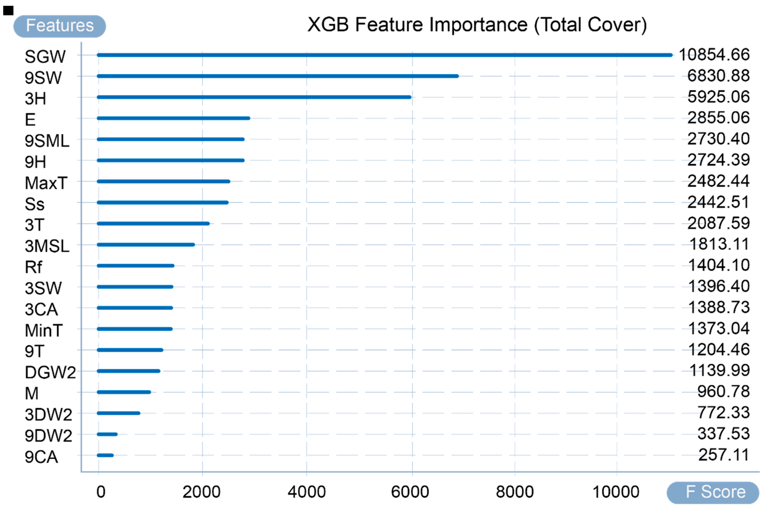
Figure 5 shows the calculated importance of input variables in the adopted dataset. The graph provides a global explanation, and its calculation factors are weight, gain, and coverage (WG&C). Weight counts the number of times a variable is used as a division variable in all trees. For example, as the highest value in this calculation method, SGW (speed of maximum wind gust) was used to divide the tree a total of 245 times. As shown in Figure 5, all variables can be divided into five echelons. The three variables of the first echelon—SGW, 3H and 9SW—are used as important features for tree division. Gain refers to the average value of the gain brought by the existence of a feature split node in all trees. For example, the average gain of 9SW (9 a.m. wind speed) ranked second in all trees is 3.864103. The larger the gain value, the smaller the loss function for the node and the model complexity in the subsequent round. In Figure 6, all variables can be divided into three echelons: the first and second echelons are SGW and 9SW, respectively, and the remaining variables are the third echelon. Figure 7 shows the coverage of each variable in the model, which refers to the average of the number of samples covered by this variable in all trees when a feature exists as a split node. For example, the third-place 3SW (3 p.m. wind speed) covers an average of 31.736 samples. It can be divided into two gradients; the first gradient is SGW and 9SW, the average value of which is much higher than the other values. The remaining variable is the second gradient.
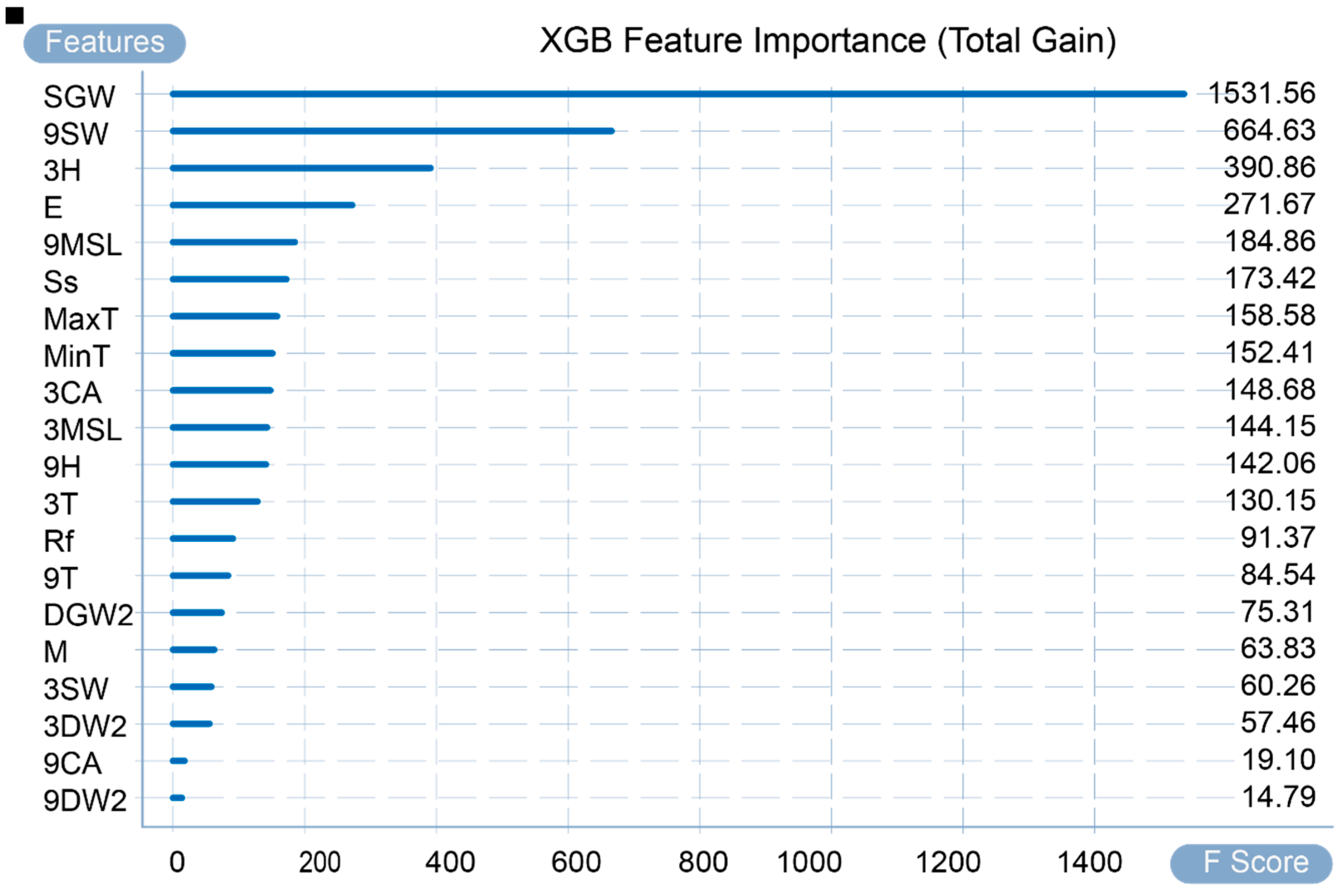
Figure 8 and Figure 9, respectively, present the total gain brought by the gain calculation method and the total number of samples obtained by the coverage calculation method. In summary, under the three calculation methods, the two variables SGW and 9SW play a very critical role in the prediction results. Therefore, it can also be seen that the occurrence of incidents and accidents mainly depends on wind speed. Other variables, such as 3H, E, and 9MSL, have a higher importance in some calculation methods. It can also be concluded that in some cases, the occurrence of incidents and accidents is also highly sensitive to humidity, evaporation, and MSL pressure.
5. Post-Hoc Local Explanation Generation
In this chapter, the XGboost model and prediction results are explained through SHAP and LIME explanations models, which, in addition to providing strong explainability and legibility, also provide an explanation of the trained predictive model and specific predictive target, local explanation, and global explanation.
5.1. SHAP Explanation
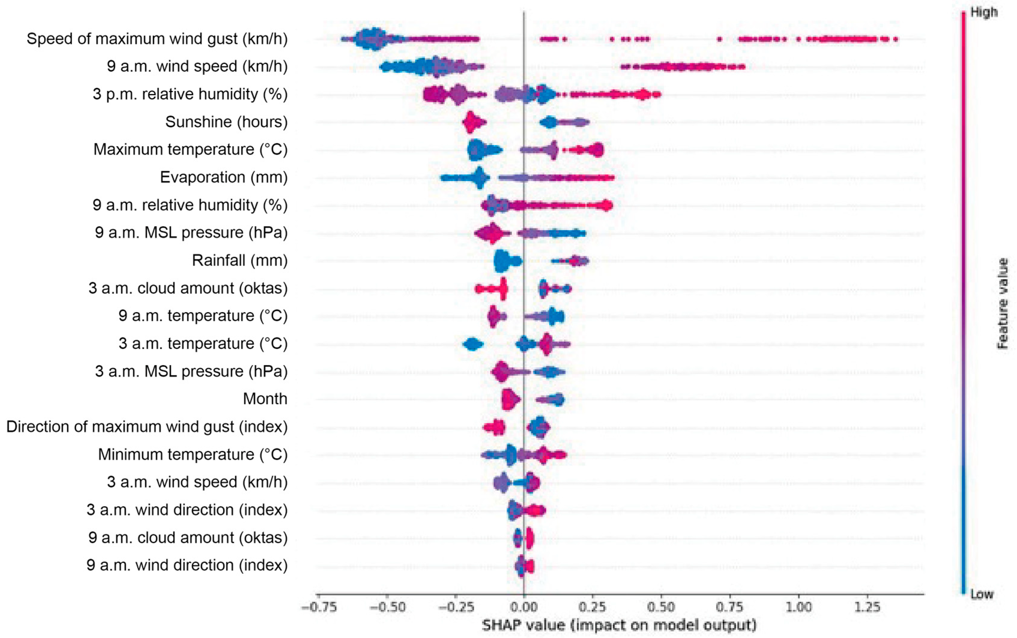
All variables in the model are considered as contributors. The importance of the SHAP value is to assign predicted values to all contributing features. To have a better global understanding of the features in the model, the summary plot is usually analysed first. The summary plot provides a visual ordering of the results by colour and coordinate axes, as presented in Figure 10. A dot in the graph represents each piece of data for each variable. The redder the colour of the dot, the larger the actual value. Contrarily, the bluer the colour, the smaller the actual value. The distribution along the Y-axis represents the data’s features, while the X-axis is the SHAP value composed of the colour system and the data dots. The jitter overlap of the data dots on the Y-axis combines the distribution of the SHAP value of each feature. Besides, the features are sorted on the Y-axis. On the X-axis, the model impact is sorted from high to low. For instance, the maximum wind gust and the wind speed at 9 a.m. greatly influence the forecast results. The higher the wind speed, the greater the forecast’s positive impact and the higher the SHAP value. Contrastingly, low wind speed has a negative impact on the result. In addition, the higher the value of sunshine time and MSL pressure, the greater the negative impact on model prediction, while the lower the actual value, the higher the SHAP value. Furthermore, it can be seen from the distribution range of the data on the X-axis that the influence of wind speed on the prediction results is much stronger than sunshine time and MSL pressure. Therefore, a preliminary conclusion can be drawn that no matter how high the value of the sunshine time and the average sea-level pressure are, as long as there is a strong wind, there will be a high probability of incidents and accidents.
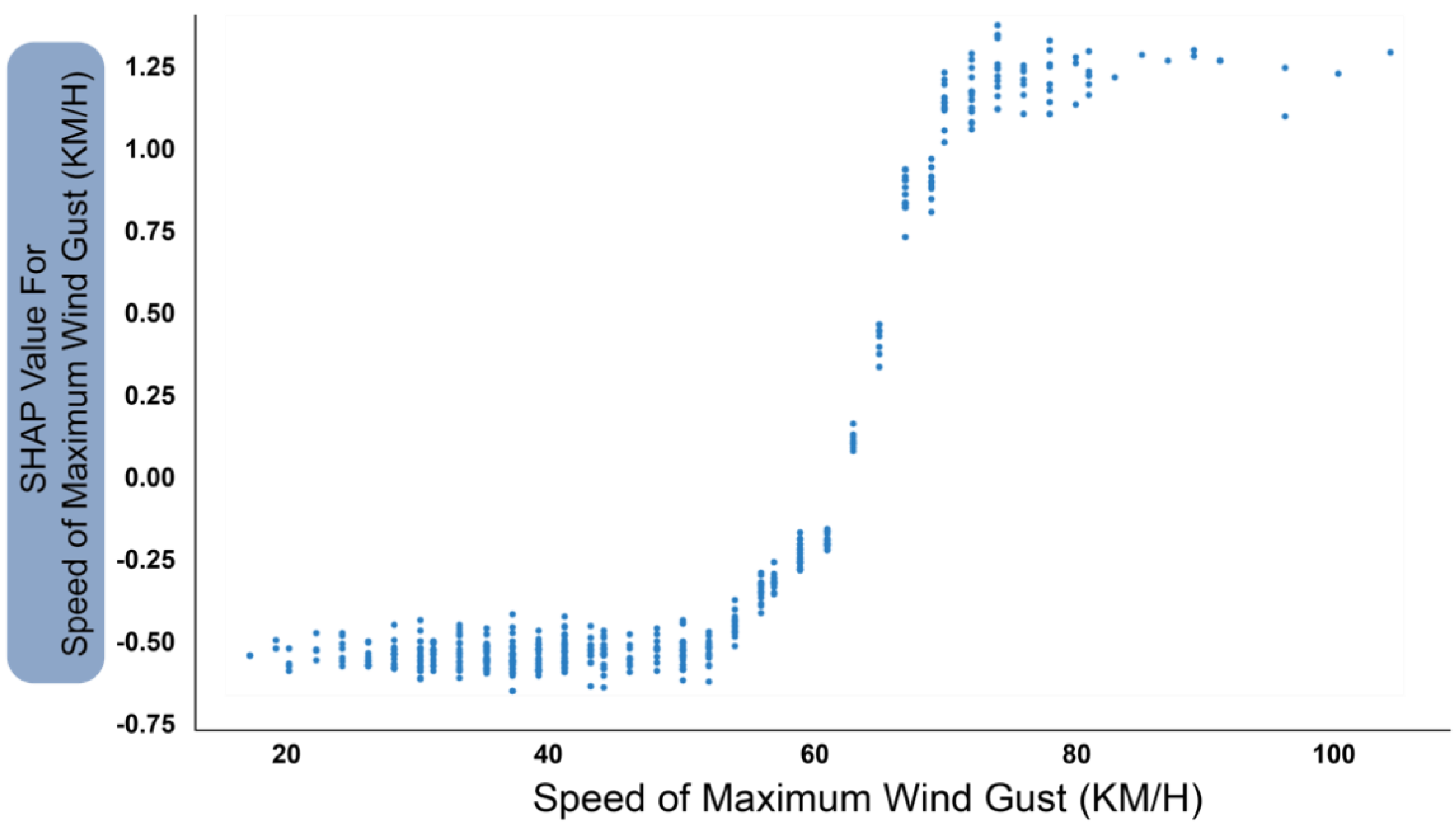
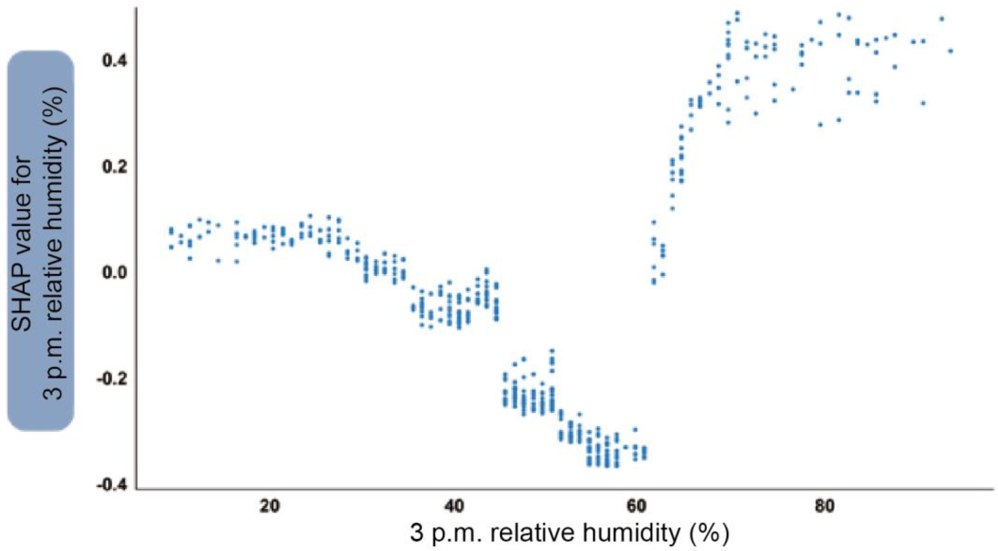
Figure 11 and Figure 12 are SHAP dependence plots that present feature dependency. Compared with the summary graph, the dependency graph is a more specific local explanation. It focuses on the impact of a single variable on the overall inference. For each data instance, a point is drawn with a characteristic value on the X-axis, and a corresponding Shapley value is drawn on the Y-axis.
Figure 11 shows the SHAP feature-dependence plot for maximum wind gust speed. Taking the wind speed of 60 km/h as the dividing line, when the wind gust speed exceeds this value, the output of the SHAP characteristic value will rise rapidly. However, when it reaches 70 km/h, no matter how the wind speed value increases, the contribution to the forecast value will no longer continue to increase. In other words, wind gust speeds exceeding 70 km/h tend to cause the same hazard to aircraft. Figure 12 shows the humidity at 3 p.m. The influence of humidity is divided into two trends and three states. The first trend is that when the humidity is lower than 60%, the contribution to incidents and accidents is continuously reduced to a negative number. Once this value is exceeded, its impact will increase rapidly. The three intervals are humidity from 0 to 40%, 40% to 60% and greater than 60%. When the humidity is 0–40%, there is no impact on incidents and accidents. when the humidity is 40–60%, the impact is negative. In other words, this humidity is statistically associated with reduced occurrences of incidents and accidents. When it is greater than 60%, the risk rises sharply, and when it reaches 70% and higher values, it will contribute noticeably to the occurrence of incidents and accidents.
5.2. LIME Explanation
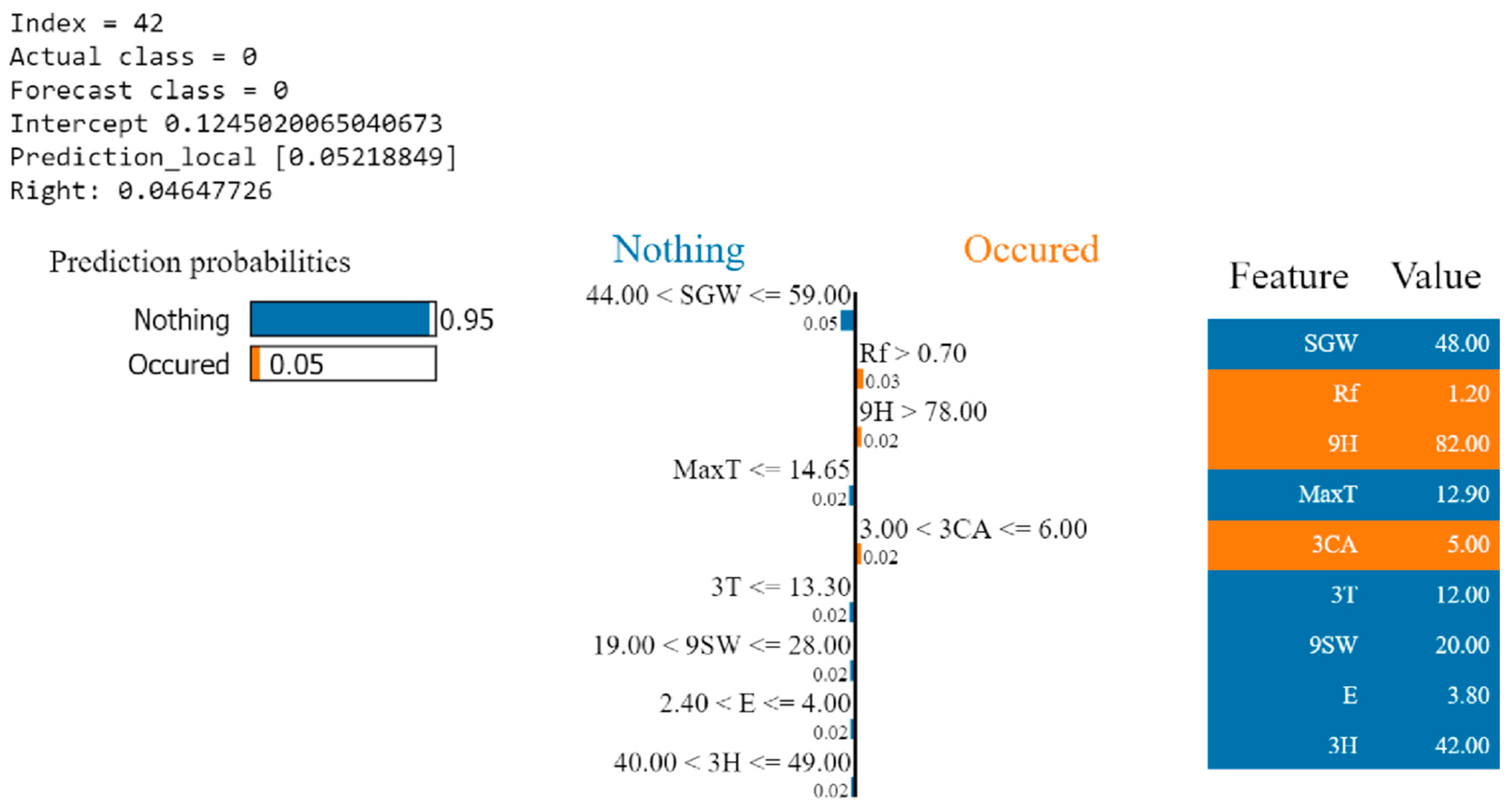
LIME can be used to show the explanation of the output of a single sample. Figure 13 and Figure 14, respectively, illustrate the predicted probabilities and detailed explanations of samples 42 and 154 in the test set. As shown in Figure 13, the XGBoost model predicts that the probability of incidents and accidents is 4.6%. LIME’s predicted probability is 5.2%. The centre plot shows the contribution of the main features corresponding to the linear model weight to the prediction. When the wind gust speed is greater than 44 km/h and less than or equal to 59 km/h, it will have a negative impact on the probability of incidents and accidents. This is also similar to the explanation given by the SHAP feature-dependence plot.
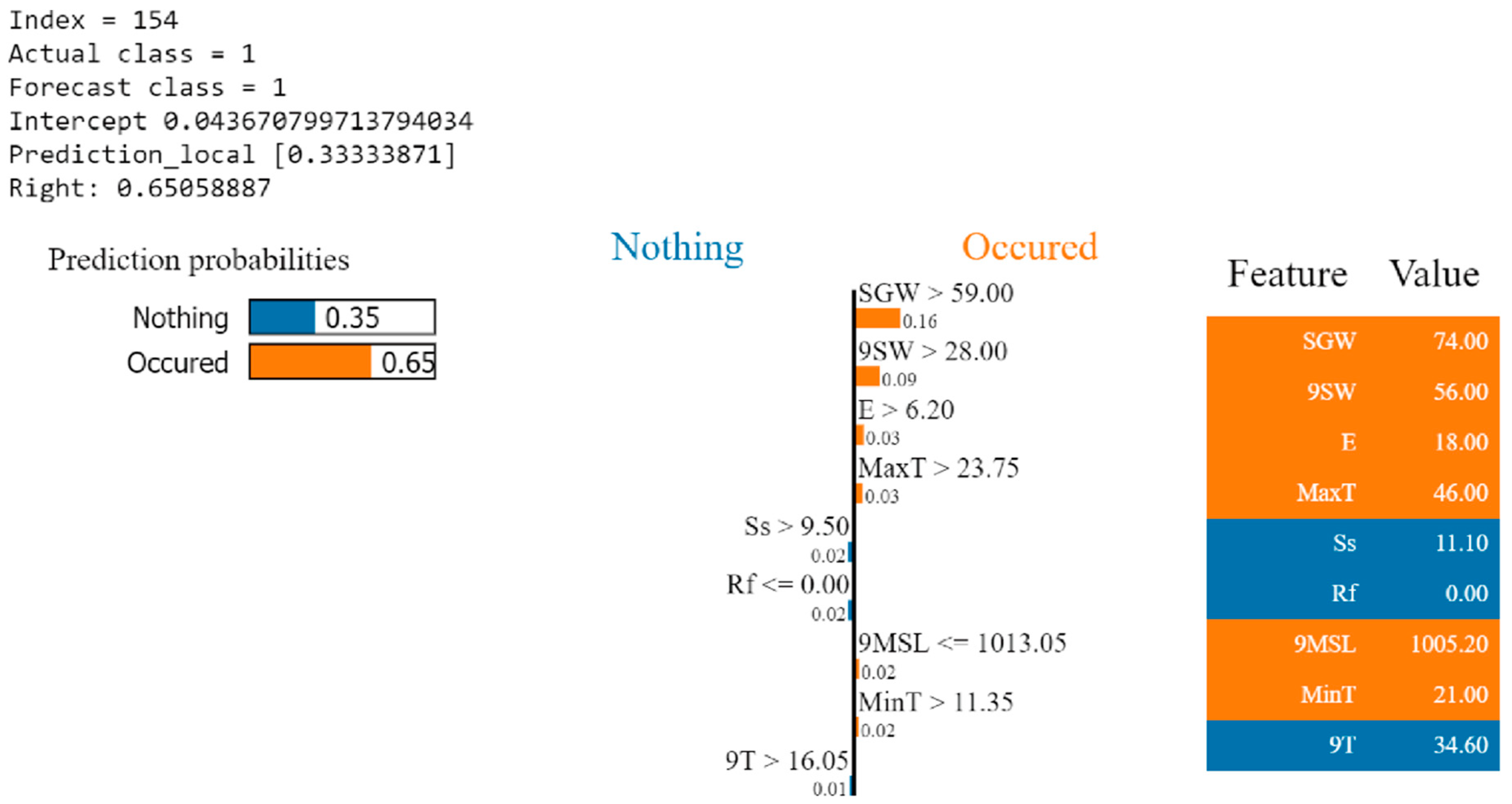
The prediction shown in Figure 14 is that incidents and accidents may occur. The XGBoost model has a prediction probability of 65%, while the LIME linear regression model has a prediction probability of only 33.3%. It shows that gusts of 74 km/h contribute the most in terms of relative weight. When 9SW is greater than 28 km/h, it has a positive contribution to the predicted result. This can also be confirmed with the SHAP explanation.
6. Model-Explanation Interface Concept
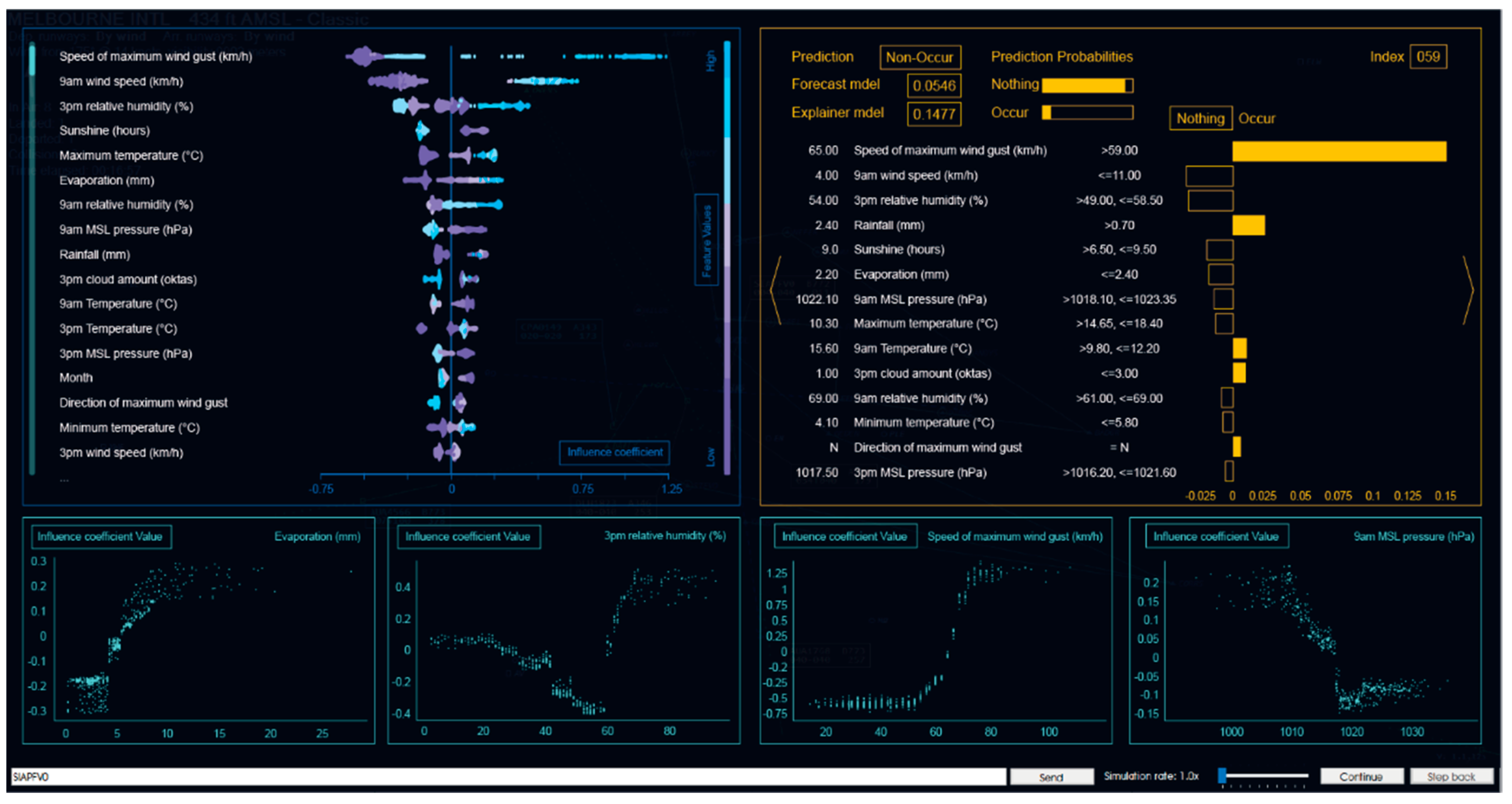
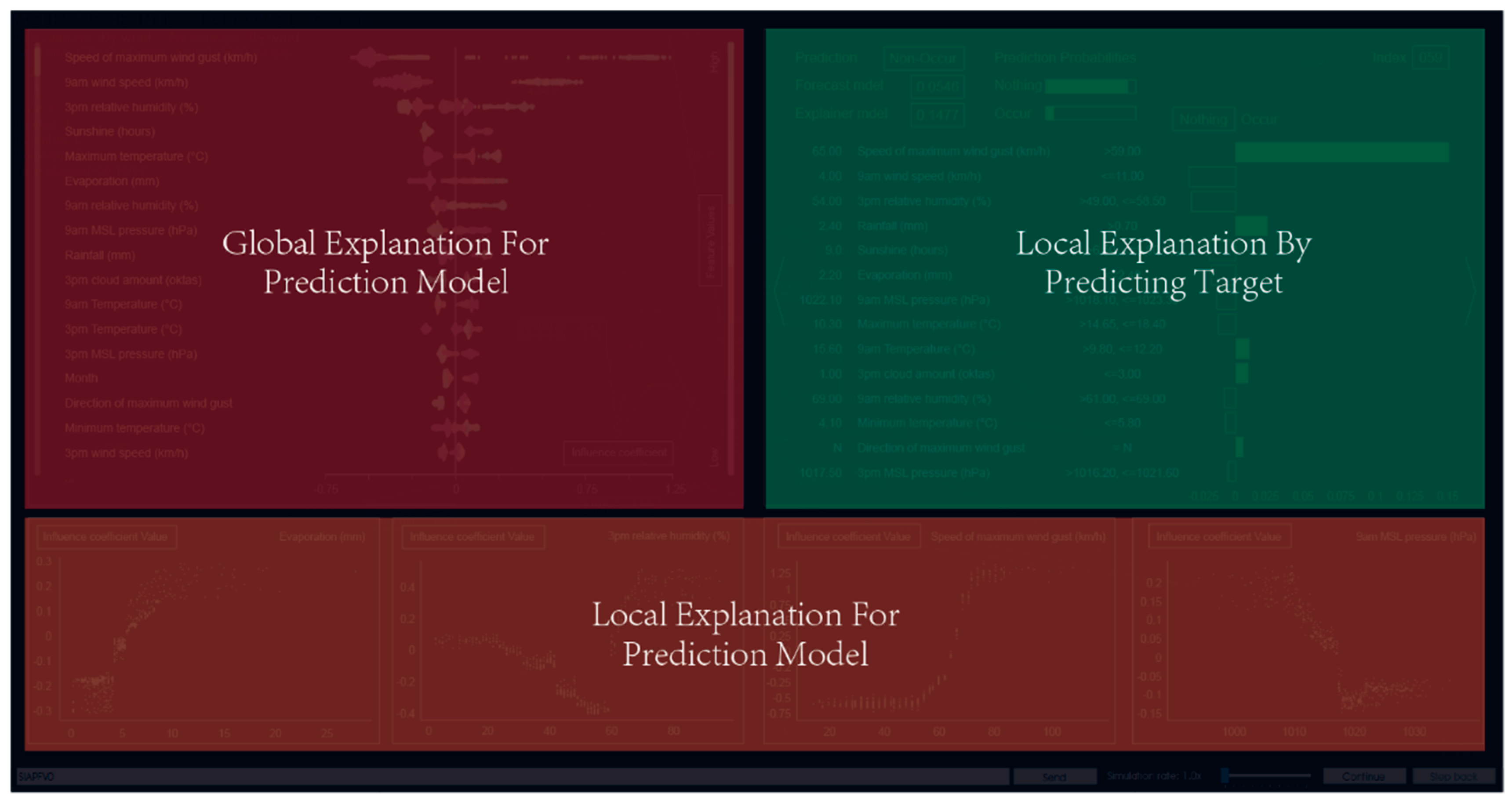
This section presents an HMI concept for ATM advisory DSS based on post-hoc explanation models, i.e., SHAP and LIME. The proposed interface is flexible and applicable in both ATM/UTM DSS; however, the concepts presented here are specifically designed for the case-study application documented in this article, which is the hypothetical risk-prediction DSS for air-traffic advisory services. The proposed graphical user interface (GUI) to present the explanations to the operator is illustrated in Figure 15. This interface shows a detailed explanation for both global and local scales. This interface is meant to be displayed on the secondary monitor and does not clutter the tactical situation display on the primary monitor. The display layout is divided into three parts, as shown in Figure 16. The red part illustrates the global explanation of the training model, that is, explaining the weight and priority of each feature after the model is trained, which is similar to the summary plot of SHAP. This information can be viewed at any time. Moreover, ATCO can allow the viewing of more feature information by sliding up and down.
The orange area at the bottom presents the local explanation of the training model detailing the relative distribution and weight of the specified features in the training model. The display of this section is not fixed, and ATCO necessitates clicking on the feature list in the red area. Up to four local feature explanations can be displayed at the same time, and they are arranged sequentially from right to left, as data can be displayed without dragging the features.
The green area on the right explains the prediction results in individual cases. Differently from the explanation based on the training model, the explanation for individual prediction is updated in real time. On the upper right of the area is the data sequence. In addition to the results of the system model, the prediction results of the explanation model are also given. The prediction results are evaluated through two different algorithm models. In the data-list section, the feature name and the real-time value of the feature are provided. The figure on the right shows the weight coefficient of the feature under the current value.
The proposed interaction mode aims to support ATCO to inspect this new information without excessively affecting the usage habits and working environment. The design of this HMI mainly focusses on the following three key points:
- Monitoring of automated processing;
- Awareness of anomalies and abnormal states; and
- Handling of emergencies.
Therefore, the information interaction of the hypothetical risk-prediction DSS is divided into two states and three modes. The two states are Predict Non-Incidents and Accidents (PNIA) and Predict Occur Incidents and Accidents (POIA). The three methods are as follows:
- Silent mode: when the prediction of incidents and accidents is below the safety threshold;
- Prompt mode: when the probability of incident or accident is above the safety threshold; and
- Detailed information mode: this can be viewed regardless of status.
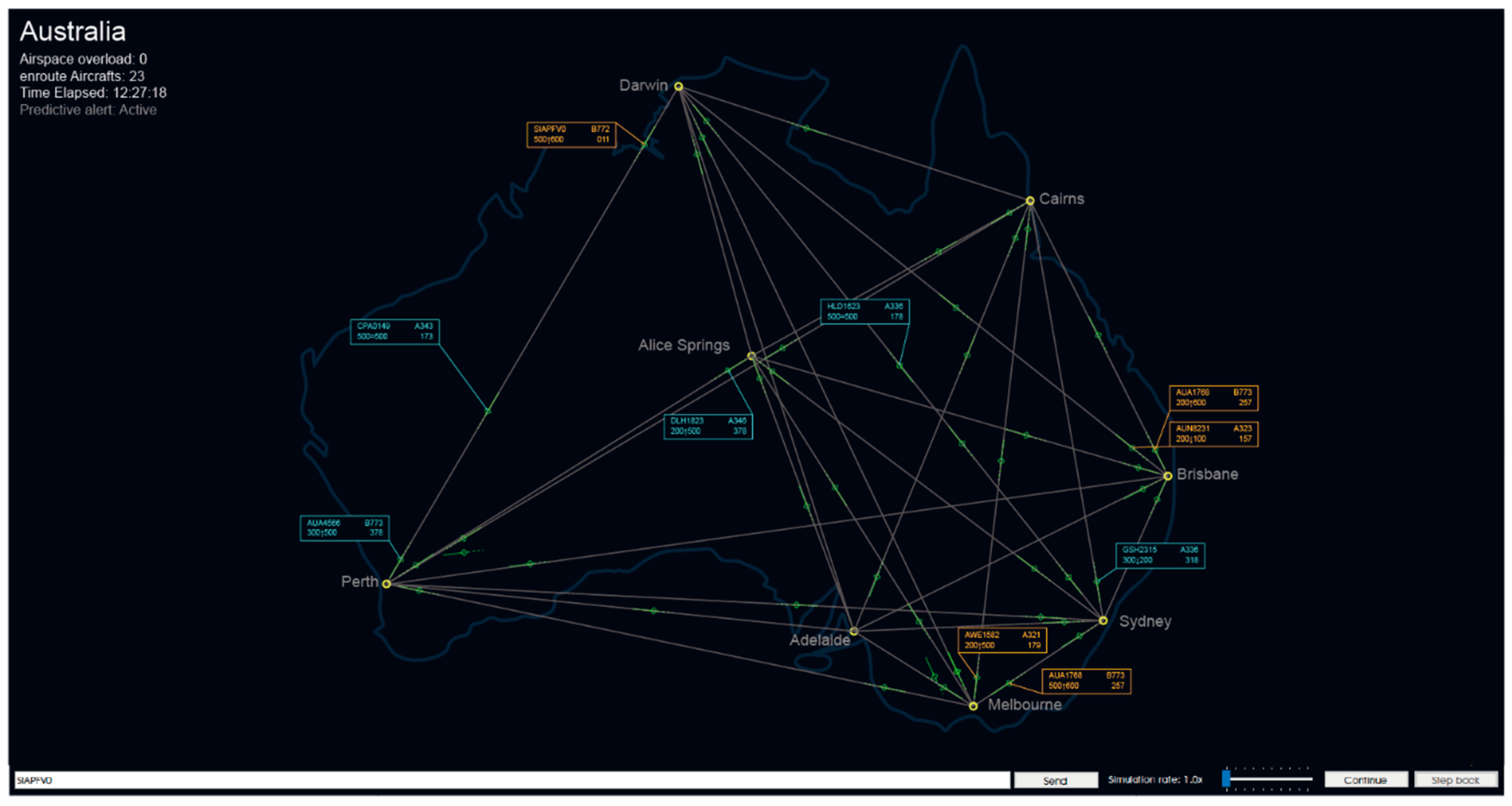
This state, depicted in Figure 17, is adopted by the system when no significant risks are predicted, and the advisory DSS is in silent mode. In this state and mode, the system will display “Predictive Alert: Active” in the information list area (top left of the main screen) and make predictions periodically. As long as the system predicts that there is no risk, the DSS will maintain this mode, which is characterised by no specific displayed information to hinder or distract ATCO’s attention.
The mode of the system is switched from silent mode to prompt mode whenever the system predicts a nonnegligible risk of incidents. Figure 18 and Figure 19 depict the visual interaction in prompt mode. Within the information list area, “Predictive Alert” changes from “Active” to “Warning” and flashes the alert. In parallel, the tag associated with the aircraft flickers to guide the ATCO to deal with emergencies.
The results of the prediction system are shown in Figure 20. Based on the original information, the label is extended to include the predicted probability of incident/accident and the type of incident/accident predicted. At the same time, it also prompts ATCO to inform the pilot. In order to open the information on the label, the system needs to receive ATCO control inputs. The input method is the mouse click, which requires ATCO to click on the label of a single aircraft with the mouse to view more information and end the flashing and alarm prompts.
7. Conclusions and Future Research
The foreseen proliferation of conventional air traffic and unmanned aircraft system (UAS) operations, particularly in low altitude airspace, prompts the need to increase the level of automation and also exploit the unique strengths of artificial intelligence (AI) and machine learning (ML). Due to the lack of transparency of the black-box model that characterises a wide variety of AI/ML algorithms, it is essential to develop strategies to ensure the explainability of decision-support system (DSS) resolutions. This paper presented the integration of a relatively conventional ML predictive model, XGBoost, with both global and local explanations methodologies, SHapley Additive exPlanations (SHAP) and Local Interpretable Model-Agnostic Explanations (LIME). The proposed solution was verified through a representative case study addressing an hypothetical, advisory DSS for real-time risk-prediction in uncontrolled airspace, for which the relative importance of various weather factors on the probability of accidents and incidents was assessed. Due to the insufficient availability of UAS-traffic data, the presented verification addressed conventional traffic in controlled airspace with risk prediction based on meteorological data. The prediction results of the XGBoost model applied to this particular case study are well within the acceptable range and show an overall high accuracy, confirming the ML model’s reliability. The SHAP and LIME algorithms are applied to the trained XGBoost model and are able to identify and illustrate very clearly the significant correlations in the dataset and how individual variables affect the prediction both locally and globally.
This research has established a feasible method to improve human-autonomy teaming by introducing explainability for AI inference processes in DSS for traditional air-traffic management (ATM) and UAS-traffic management (UTM). However, the methods described in this article have been so far verified only in the hypothetical DSS for advisory services. In our future work, we will focus on integrating AI algorithm-interpretation methods into the development stage of algorithms and systems, extending the proposed interpretation framework to other applications or use other forms of AI to improve mutual trust between humans and intelligent systems.
Supplementary Materials
The following are available online at https://www.mdpi.com/article/10.3390/aerospace8080224/s1, Supplementary Data.
Author Contributions
Conceptualisation and methodology, Y.X., N.P. and A.G.; software, Y.X.; writing—original draft preparation, Y.X. and N.P.; writing—review and editing, A.G. and R.S.; supervision, A.G. and R.S.; project administration, R.S. and A.G. All authors have read and agreed to the published version of the manuscript.
Funding
This research received no external funding.
Institutional Review Board Statement
Not applicable.
Informed Consent Statement
Not applicable.
Data Availability Statement
Conflicts of Interest
The authors declare no conflict of interest.
Appendix A
To prevent overfitting, the algorithm adds L1 and L2 regularisation terms by having the objective function that sums regularisation and loss function , while is a parameter trained from a set of given data, as shown in Equation (A1).
The objective function of the model is presented in Equation (A2). The first part is the training loss, which represents the difference between the real value and the predicted value. The second part is the regularisation, which is used to control the complexity of the tree.
Equation (A3) is the optimised tree, where (time iteration) is defined as the sum of the scores. Equation (A4) is the obtained objective function formula.
Taylor expansion is performed on the objective function and combines Equations (A3) and (A4) to get Equation (A5).
Equation (A6) is the regularisation formula, where is the complexity parameter of each leaf; is the number of leaves; is the parameter to measure the penalty; is the vector of scores on the leaves. Equation (A7) defines as the node of the leaf and is the weight of the leaf, which is the value of the leaf node.
When removing all constant values, Equations (A6) and (A7) are combined to get the objective function as Equations (A8) and (A9).
when and , the equation changes to Equation (A10).
To obtain the best value of each leaf node and the corresponding objective function value, Equation (A10) is optimised by the following Equations (A11) and (A12):
When CART continues to branch until the tree grows to the maximum depth, Equation (A13) is then used to determine the stop gain. Equation (A13) comprises four parts: the score on the new right leaf, the score on the new left leaf, the score on the original leaf, and the regularised on the additional leaf.
References
- Gosling, G.D. Identification of artificial intelligence applications in air traffic control. Transp. Res. Part A Gen. 1987, 21, 27–38. [Google Scholar] [CrossRef]
- Crespo, A.M.F.; Weigang, L.; de Barros, A.G. Reinforcement learning agents to tactical air traffic flow management. Int. J. Aviat. Manag. 2012, 1, 145–161. [Google Scholar] [CrossRef]
- Gardi, A.; Sabatini, R.; Ramasamy, S. Multi-objective optimisation of aircraft flight trajectories in the ATM and avionics context. Prog. Aerosp. Sci. 2016, 83, 1–36. [Google Scholar] [CrossRef]
- Kistan, T.; Gardi, A.; Sabatini, R.; Ramasamy, S.; Batuwangala, E. An evolutionary outlook of air traffic flow management techniques. Prog. Aerosp. Sci. 2017, 88, 15–42. [Google Scholar] [CrossRef]
- Pongsakornsathien, N.; Bijjahalli, S.; Gardi, A.; Symons, A.; Xi, Y.; Sabatini, R.; Kistan, T. A Performance-Based Airspace Model for Unmanned Aircraft Systems Traffic Management. Aerospace 2020, 7, 154. [Google Scholar] [CrossRef]
- Kistan, T.; Gardi, A.; Sabatini, R. Machine Learning and Cognitive Ergonomics in Air Traffic Management: Recent Developments and Considerations for Certification. Aerospace 2018, 5, 103. [Google Scholar] [CrossRef] [Green Version]
- Borst, C.; Bijsterbosch, V.A.; Van Paassen, M.M.; Mulder, M. Ecological interface design: Supporting fault diagnosis of automated advice in a supervisory air traffic control task. Cogn. Technol. Work. 2017, 19, 545–560. [Google Scholar] [CrossRef]
- Borghini, G.; Aricò, P.; Di Flumeri, G.; Cartocci, G.; Colosimo, A.; Bonelli, S.; Golfetti, A.; Imbert, J.P.; Granger, G.; Benhacene, R.; et al. EEG-Based Cognitive Control Behaviour Assessment: An Ecological study with Professional Air Traffic Controllers. Sci. Rep. 2017, 7, 547. [Google Scholar] [CrossRef]
- Diffenderfer, P.; Tao, Z.; Payton, G. Automated integration of arrival/departure schedules. In Proceedings of the Tenth USA/Europe Air Traffic Management Seminar, Chicago, IL, USA, 10–13 June 2013. [Google Scholar]
- Hagras, H. Toward Human-Understandable, Explainable AI. Computer 2018, 51, 28–36. [Google Scholar] [CrossRef]
- Sheh, R.; Monteath, I. Defining Explainable AI for Requirements Analysis. KI Künstliche Intell. 2018, 32, 261–266. [Google Scholar] [CrossRef]
- SESAR. JU Webinar: Artificial Intelligence in ATM (Part 2); SESAR (YouTube Channel). 2020. Available online: https://www.youtube.com/watch?v=p_8o8iuc3A0&t=401s (accessed on 2 September 2020).
- Arrieta, A.B.; Díaz-Rodríguez, N.; Del Ser, J.; Bennetot, A.; Tabik, S.; Barbado, A.; Garciag, S.; Gil-Lopeza, S.; Molinag, D.; Benjaminsh, R.; et al. Explainable Artificial Intelligence (XAI): Concepts, Taxonomies, Opportunities and Challenges toward Responsible. AI. Inf. Fusion 2020, 58, 82–115. [Google Scholar] [CrossRef] [Green Version]
- Zhu, J.; Liapis, A.; Risi, S.; Bidarra, R.; Youngblood, G.M. Explainable AI for Designers: A Human-Centered Perspective on Mixed-Initiative Co-Creation. In Proceedings of the 2018 IEEE Conference on Computational Intelligence and Games (CIG), Maastricht, The Netherlands, 14–17 August 2014; pp. 1–8. [Google Scholar]
- Stephen, M. Open-Source AI Bionic Leg Offers a Unified Platform for Prosthetics. Machine Design. 2019. Available online: https://www.machinedesign.com/mechanical-motion-systems/article/21837881/opensource-ai-bionic-leg-offers-a-unified-platform-for-prosthetics (accessed on 14 October 2020).
- Huang, C.; Mezencev, R.; McDonald, J.F.; Vannberg, F. Open source machine-learning algorithms for the prediction of optimal cancer drug therapies. PLoS ONE 2017, 12, e0186906. [Google Scholar] [CrossRef] [Green Version]
- Waller, S.; Chiu, Y.-C.; Ruiz-Juri, N.; Unnikrishnan, A.; Bustillos, B.I. Short Term Travel Time Prediction on Freeways in Conjunction with Detector Coverage Analysis. Available online: https://trid.trb.org/view/859411 (accessed on 31 July 2021).
- Karlaftis, M.; Vlahogianni, E. Statistical methods versus neural networks in transportation research: Differences, similarities and some insights. Transp. Res. Part C Emerg. Technol. 2011, 19, 387–399. [Google Scholar] [CrossRef]
- Botzoris, G.N.; Profillidis, V.A. Modeling of Transport Demand: Analyzing, Calculating, and Forecasting Transport Demand; Elsevier: St. Louis, MO, USA, 2018. [Google Scholar]
- Kwon, J.; Coifman, B.; Bickel, P. Day-to-Day Travel-Time Trends and Travel-Time Prediction from Loop-Detector Data. Transp. Res. Rec. J. Transp. Res. Board 2000, 1717, 120–129. [Google Scholar] [CrossRef]
- Ma, X.; Tao, Z.; Wang, Y.; Yu, H.; Wang, Y. Long short-term memory neural network for traffic speed prediction using remote microwave sensor data. Transp. Res. Part C Emerg. Technol. 2015, 54, 187–197. [Google Scholar] [CrossRef]
- Elith, J.; Leathwick, J.R.; Hastie, T. A working guide to boosted regression trees. J. Anim. Ecol. 2008, 77, 802–813. [Google Scholar] [CrossRef]
- Zhang, Y.; Haghani, A. A gradient boosting method to improve travel time prediction. Transp. Res. Part C Emerg. Technol. 2015, 58, 308–324. [Google Scholar] [CrossRef]
- Dalmau, R.; Ballerini, F. Improving the Predictability of Take-off Times with Machine Learning. In Proceedings of the 9th SESAR Innovation Days, Athens, Greece, 2–5 December 2019; Available online: https://www.sesarju.eu/sites/default/files/documents/sid/2019/papers/SIDs_2019_paper_36.pdf (accessed on 3 October 2020).
- Liang, W.; Luo, S.; Zhao, G.; Wu, H. Predicting Hard Rock Pillar Stability Using GBDT, XGBoost, and LightGBM Algorithms. Mathematics 2020, 8, 765. [Google Scholar] [CrossRef]
- Gu, X.; Han, Y.; Yu, J. A Novel Lane-Changing Decision Model for Autonomous Vehicles Based on Deep Autoencoder Network and XGBoost. IEEE Access 2020, 8, 9846–9863. [Google Scholar] [CrossRef]
- Lundberg, S.M.; Erion, G.; Chen, H.; DeGrave, A.; Prutkin, J.M.; Nair, B.; Katz, R.; Himmelfarb, J.; Bansal, N.; Lee, S.-I. Explainable AI for Trees: From Local Explanations to Global Understanding. arXiv 2019, arXiv:1905.04610. [Google Scholar] [CrossRef]
- Beyer, R. HMI Aspects of Support Tools for Air Traffic Management. IFAC Proc. Vol. 2001, 34, 549–553. [Google Scholar] [CrossRef]
- Arico, P.; Borghini, G.; Di Flumeri, G.; Bonelli, S.; Golfetti, A.; Graziani, I.; Pozzi, S.; Imbert, J.-P.; Granger, G.; Benhacene, R.; et al. Human Factors and Neurophysiological Metrics in Air Traffic Control: A Critical Review. IEEE Rev. Biomed. Eng. 2017, 10, 250–263. [Google Scholar] [CrossRef] [PubMed]
- Ødegård, S.S. Exploring Visualization—Solutions for Air Traffic Control Workflow Productivity Improvement. Master’s Thesis, Department of Informatics, University of Oslo, Oslo, Norway, 2013. Available online: https://www.duo.uio.no/handle/10852/37418 (accessed on 1 October 2020).
- Bourgois, M.; Cooper, M.; Duong, V.; Hjalmarsson, J.; Lange, M.; Ynnerman, A. Interactive and immersive 3D visualization for ATC. In Proceedings of the 3rd Eurocontrol Innovative Research Workshop, Paris, France, 6–8 December 2005. [Google Scholar]
- ICAO. Human Factors Training Manual; ICAO: Montreal, QC, Canada, 1998. [Google Scholar]
- Lim, Y.; Ramasamy, S.; Gardi, A.; Kistan, T.; Sabatini, R. Cognitive Human-Machine Interfaces and Interactions for Unmanned Aircraft. J. Intell. Robot. Syst. 2018, 91, 755–774. [Google Scholar] [CrossRef]
- Lim, Y.; Gardi, A.; Sabatini, R.; Ramasamy, S.; Kistan, T.; Ezer, N.; Vince, J.; Bolia, R. Avionics Human-Machine Interfaces and Interactions for Manned and Unmanned Aircraft. Prog. Aerosp. Sci. 2018, 102, 1–46. [Google Scholar] [CrossRef]
- Pongsakornsathien, N.; Lim, Y.; Gardi, A.; Hilton, S.; Planke, L.; Sabatini, R.; Kistan, T.; Ezer, N. Sensor Networks for Aerospace Human-Machine Systems. Sensors 2019, 19, 3465. [Google Scholar] [CrossRef] [Green Version]
- Chen, T.; Guestrin, C. XGBoost: A Scalable Tree Boosting System. In Proceedings of the 22nd ACM SIGKDD International Conference on Knowledge Discovery and Data Mining, San Francisco, CA, USA, 13–17 August 2016; pp. 785–794. [Google Scholar]
- Patidar, P.; Tiwari, A. Handling Missing Value in Decision Tree Algorithm. Int. J. Comput. Appl. 2013, 70, 31–36. [Google Scholar] [CrossRef] [Green Version]
- Ribeiro, M.T.; Singh, S.; Guestrin, C. Why Should I Trust You?: Explaining the Predictions of Any Classifier. In Proceedings of the 22nd ACM SIGKDD International Conference on Knowledge Discovery and Data Mining, San Francisco, CA, USA, 13–17 August 2016; pp. 1135–1144. [Google Scholar]
- Strumbelj, E.; Kononenko, I. An Efficient Explanation of Individual Classifications using Game Theory. J. Mach. Learn. Res. 2010, 11, 1–18. [Google Scholar] [CrossRef]
- Zhao, W.; Joshi, T.; Nair, V.N.; Sudjianto, A. SHAP values for Explaining CNN-based Text Classification Models. arXiv 2020, arXiv:2008.11825. [Google Scholar]
- Chen, Y. Understanding Machine Learning Classifier Decisions in Automated Radiotherapy Quality Assurance; ProQuest Dissertations Publishing: Ann Arbor, MI, USA, 2020. [Google Scholar]
- Meteorology B o. Daily Weather Observations. Available online: http://www.bom.gov.au/climate/dwo/ (accessed on 24 September 2020).
- ATSB. ATSB National Aviation Occurrence Database: Advanced Search. Available online: http://data.atsb.gov.au/AdvancedSearch (accessed on 23 September 2020).
- Laurae. Ensembles of Tree-Based Models: Why Correlated Features Do Not Trip Them—And Why NA Matters. Available online: https://medium.com/data-design/ensembles-of-tree-based-models-why-correlated-features-do-not-trip-them-and-why-na-matters-7658f4752e1b (accessed on 28 September 2016).
Figure 1.
Classication of explainable artifical intellengence methods.

Figure 2.
Example of CART prediction.

Figure 3.
Process framework of the prediction model.

Figure 4.
Correlations of each feature.

Figure 5.
Feature importance by weight.

Figure 6.
Feature importance by gain.

Figure 7.
Feature importance by coverage.

Figure 8.
Feature importance for total gain.

Figure 9.
Feature importance for total coverage.

Figure 10.
SHAP explanation of the summary plot.

Figure 11.
SHAP explanation of dependence plot for speed of max wind gust.

Figure 12.
SHAP explanation of dependence plot for 3 p.m. relative humidity.

Figure 13.
LIME explanation for a sample No. 42.

Figure 14.
LIME explanation for a sample of No. 154.

Figure 15.
Explanation interface concept.

Figure 16.
The layout of the detailed explanation interface concept.

Figure 17.
Silent mode interface concept.

Figure 18.
Visual interaction in prompt mode at the top left corner.

Figure 19.
Visual interaction in prompt mode in the central display area.

Figure 20.
Detailed visual interaction in prompt mode.


Table 1.
The features and differences between LIME and SHAP.
| LIME | SHAP | |
|---|---|---|
| Features | Local Explaination Method; Does not interface with the algorithm inside the black box; Independently generates new samples based on each feature. | Local Explaination Method; Based on game theory; Calculates the importance of additive features for each specific prediction. |
| Advantage | Model-Agnositc method; even if the prediction model changes, LIME is able to make the local explanation. | Supports multiple explain plots; Allows comparative studies between features; Can quickly implement and explain tree-based models. |
| Disadvantage | The explained results are not stable enough, and different interpretation models will produce different results. | Long calculation time, slower interpretation production speed. |
Table 2.
(a) Full names to the abbreviations. (b) Wind direction codes.
| (a) Full Names to the Abbreviations | |||
|---|---|---|---|
| Abbreviation | Full Name | Abbreviation | Full Name |
| M | Month | 9DW | 9 a.m. wind direction |
| MinT | Minimum temperature (°C) | 9DW2 | 9 a.m. wind direction (index) |
| MaxT | Maximum temperature (°C) | 9SW | 9 a.m. wind speed (km/h) |
| Rf | Rainfall (mm) | 9MSL | 9 a.m. MSL pressure (hPa) |
| E | Evaporation (mm) | 3T | 3 p.m. Temperature (°C) |
| Ss | Sunshine (hours) | 3H | 3 p.m. relative humidity (%) |
| DGW | Direction of maximum wind gust | 3CA | 3 p.m. cloud amount (oktas) |
| DGW2 | Direction of maximum wind gust (index) | 3DW | 3 p.m. wind direction |
| SGW | Speed of maximum wind gust (km/h) | 3DW2 | 3 p.m. wind direction (index) |
| 9T | 9 a.m. temperature (°C) | 3SW | 3 p.m. wind speed (km/h) |
| 9H | 9 a.m. relative humidity (%) | 3MSL | 3 p.m. MSL pressure (hPa) |
| 9CA | 9 a.m. cloud amount (oktas) | IA | Incident and accident (Binary) |
| (b) Wind Direction Codes | |||
| Code | Wind Direction | Code | Wind Direction |
| 1 | N | 9 | S |
| 2 | NNE | 10 | SSW |
| 3 | NE | 11 | SW |
| 4 | ENE | 12 | WSW |
| 5 | E | 13 | W |
| 6 | ESE | 14 | WNW |
| 7 | SE | 15 | NW |
| 8 | SSE | 16 | NNW |
Publisher’s Note: MDPI stays neutral with regard to jurisdictional claims in published maps and institutional affiliations. |
© 2021 by the authors. Licensee MDPI, Basel, Switzerland. This article is an open access article distributed under the terms and conditions of the Creative Commons Attribution (CC BY) license (https://creativecommons.org/licenses/by/4.0/).
Share and Cite
MDPI and ACS Style
Xie, Y.; Pongsakornsathien, N.; Gardi, A.; Sabatini, R. Explanation of Machine-Learning Solutions in Air-Traffic Management. Aerospace 2021, 8, 224. https://doi.org/10.3390/aerospace8080224
AMA Style
Xie Y, Pongsakornsathien N, Gardi A, Sabatini R. Explanation of Machine-Learning Solutions in Air-Traffic Management. Aerospace. 2021; 8(8):224. https://doi.org/10.3390/aerospace8080224
Chicago/Turabian StyleXie, Yibing, Nichakorn Pongsakornsathien, Alessandro Gardi, and Roberto Sabatini. 2021. "Explanation of Machine-Learning Solutions in Air-Traffic Management" Aerospace 8, no. 8: 224. https://doi.org/10.3390/aerospace8080224
Note that from the first issue of 2016, this journal uses article numbers instead of page numbers. See further details here.