pyCycle: A Tool for Efficient Optimization of Gas Turbine Engine Cycles

NASA Glenn Research Center, Cleveland, OH 44135, USA
*
Author to whom correspondence should be addressed.
Aerospace 2019, 6(8), 87; https://doi.org/10.3390/aerospace6080087
Submission received: 24 June 2019
/
Revised: 26 July 2019
/
Accepted: 29 July 2019
/
Published: 8 August 2019
(This article belongs to the Special Issue Multidisciplinary Design Optimization in Aerospace Engineering)
Abstract
:Aviation researchers are increasingly focusing on unconventional vehicle designs with tightly integrated propulsion systems to improve overall aircraft performance and reduce environmental impact. Properly analyzing these types of vehicle and propulsion systems requires multidisciplinary models that include many design variables and physics-based analysis tools. This need poses a challenge from a propulsion modeling standpoint because current state-of-the-art thermodynamic cycle analysis tools are not well suited to integration into vehicles level models or to the application of efficient gradient-based optimization techniques that help to counteract the increased computational costs. Therefore, the objective of this research effort was to investigate the development a new thermodynamic cycle analysis code, called pyCycle, to address this limitation and enable design optimization of these new vehicle concepts. This paper documents the development, verification, and application of this code to the design optimization of an advanced turbofan engine. The results of this study show that pyCycle models compute thermodynamic cycle data within 0.03% of an identical Numerical Propulsion System Simulation (NPSS) model. pyCycle also provides more accurate gradient information in three orders of magnitude less computational time by using analytic derivatives. The ability of pyCycle to accurately and efficiently provide this derivative information for gradient-based optimization was found to have a significant benefit on the overall optimization process with wall times at least seven times faster than using finite difference methods around existing tools. The results of this study demonstrate the value of using analytic derivatives for optimization of cycle models, and provide a strong justification for integrating derivatives into other important engineering analyses.
1. Introduction
Thermodynamic cycle analysis is a fundamental technique for the analysis and design of gas turbine engines. The importance of thermodynamic cycle analysis is demonstrated by the central role the calculations hold in the engine design processes described by Saravanamutto et al. [1], Mattingly [2], Walsh and Fletcher [3], and Hendricks [4]. As described by Oates [5]: “The object of cycle analysis is to obtain estimates of the performance parameters (primarily thrust and specific fuel consumption) in terms of the design limitations (such as the maximum allowable turbine temperature), the flight conditions (the ambient pressure and temperature and the Mach number) and design choices (such as the compressor pressure ratio, fan pressure ratio, by-pass ratio, etc.).” Given this system level focus, cycle analysis is commonly one of the first steps in these design processes and is used to define the initial design for the engine. Following more detailed design of the engine components and the overall vehicle, improved component design information is fed back into the cycle analysis to ensure that the overall design can satisfy the specified performance requirements. This creates an iterative design process with cycle analysis serving as the key analysis method for initializing, guiding the development of, and then ultimately confirming the final engine design [6].
Cycle analysis techniques have been studied since the conception of the gas turbine engine in the 1930s. While the fundamental equations governing cycle analysis are rooted in the laws of thermodynamics for a steady one-dimensional flow, the implementation of these equations has changed substantially over the years. These different implementations, predominantly in the form of various computer codes, can be organized into several major eras as shown in Figure 1. This history was pieced together from several sources [6,7,8] with incomplete or conflicting information, so it should be noted that the dates defining the start and end of these eras are approximate.
Up to the 1950s, cycle analysis was primarily completed by hand as access to computing resources was extremely rare. Hand calculations were used to converge (also referred to as match) cycle models, which was feasible because engine designs were mainly relatively simple single shaft turbojet designs. As the engine designs became more complex (with more shafts, bypass configurations, or afterburners) and computing availability increased, the next era of cycle analysis implemented single-purpose cycle analysis programs. With this approach, a new cycle analysis program was developed for each engine being studied and these tools only contained the equations required for that particular engine. These programs as a result could not be easily modified to model other engine designs.
Given this limitation, the next two eras aimed to create more flexible cycle analysis tools. The third era implemented pre-configured multi-purpose tools that contained a set of pre-configured generic engine designs (architectures) that the user could select. Modeling a specific engine of that architecture was completed by supplying appropriate inputs to define the engine. This greatly increased the reusability of the code and enabled more rapid analysis of a wide range of engines, but it was still challenging to model new or unconventional designs which were not one of the pre-configured architecture options. The limitations for exploring new engine concepts spurred the fourth era in cycle analysis where modular multi-purpose tools were built to handle any possible configuration. In this era, reusable modules were written for each of the major engine components (e.g., compressors, burners, and turbines). Users could then link these modules together to form the flowpath of the particular engine they wanted to examine. Any engine configuration could now be modeled as long as the engine components required were part of the code. Moving to a modular approach significantly improved the utility of these tools for developing a wide range of engine models.
Starting in the early 1990s, a fifth cycle analysis era began with the development of Numerical Propulsion System Simulation (NPSS) [9] via a collaboration between industry and NASA. NPSS expanded on the modular structure of the previous era and also made improvements to enable multidisciplinary and multi-fidelity engine analysis [10,11]. This approach, commonly referred to as zooming, expanded the focus of cycle analysis to serve as an integrator for models of individual engine components. NPSS also incorporated emerging computer science approaches such as object-oriented programming and interpreted programming languages to improve code organization and ease of use [6]. These advancements have made NPSS the state-of-the-art for the past 20 years for cycle analysis in an engine centric design process.
However, several emerging trends in aviation research are indicating that the current engine-centric modeling paradigm will need to give way to a vehicle system focused, multidisciplinary approach. One emerging trend is the interest in greater aeropropulsive integration. For example, many conceptual vehicle designs, such as the STARC-ABL [12] and D8 [13], have proposed the use of boundary layer ingestion (BLI). In these concepts, the propulsion system is placed on the vehicle so that portions of the boundary layer are ingested by the engine. This has the potential to increase the propulsive efficiency, reduce the airframe and nacelle drag, and decrease the wake mixing losses [14]. A second emerging trend is the push toward more electric propulsion systems concepts. For example, the PEGASUS [15], N-3X [16], and STARC-ABL [12] all propose some form of more electric propulsion.
For both BLI and electric propulsion concepts, the system performance benefits are obtained by taking advantage of the physical interactions between the engine and other systems on the vehicle. In the case of BLI designs, the propulsion system and the vehicles aerodynamic design have significant aeropropulsive interactions. For the electric propulsion, the engine is closely coupled with the electrical and thermal management system designs. As a result of the strong interactions, the design of the gas turbine engine can no longer be completed in isolation from these other vehicle systems. Therefore, this paper proposes that a sixth era of cycle analysis is emerging where cycle analysis will be just one discipline within a tightly-coupled, multidisciplinary design problem for the larger vehicle system.
Incorporating cycle analysis into larger vehicle and mission system model contexts presents a number of new challenges. Physical interactions, such as the aeropropulsive interactions in BLI, often require the use of computationally-intensive, higher-order aerodynamic codes because lower-order tools do not capture all of the relevant physics. In addition, the cycle analysis and aerodynamic codes need to be tightly coupled (i.e., two-way passing of information between the disciplines with an iterative procedure used to achieve convergence [17]), further increasing the computational complexity and cost. The use of higher-order codes also demands the usage of much more detailed geometry definitions. This information is not typically known in the conceptual design phase and therefore must be included in the design space to be explored, significantly increasing the number of design variables. Hence, it becomes important to employ methods that can efficiently navigate large design spaces to find optimal candidate designs.
Despite the challenges with coupling NPSS into a vehicle level design process, there have been several notable attempts to accomplish this task. Ordaz [18] developed a multidisciplinary analysis environment that combined NPSS with the FUN3D computational fluid dynamics (CFD) solver solver to analyze BLI aircraft concepts including the STARC-ABL. Geiselhart et al. [19] developed an integrated aircraft design optimization that combined NPSS with the aircraft mission analysis tool and sizing tool FLOPS to study low-boom design for a supersonic business jet using gradient-free optimization. Allison et al. [20] published a study that investigated the integration of NPSS into an aircraft design optimization for a supersonic fighter jet, and, in follow-on work, Allison et al. [21] attempted to integrate NPSS with a high-fidelity model for nozzle installation effects. Although these studies did succeed in using NPSS in a vehicle level context, they also identified several significant limitations that they encountered. Geiselhart et al. specifically noted that computational cost and numerical stability issues with the NPSS cycle analysis model were a major motivating factor for using a gradient free optimization method. Allison et al. preferred to focus on integrated analysis models and design of experiments based methods to navigate the design space, which limited the number of design variables they could handle. Overall, these results exposed some weaknesses of NPSS in the context of vehicle system design and ultimately forced these studies to apply methods that do not scale well to problems with larger design spaces.
Although the difficulty that arises when optimizing larger design spaces is relatively new to the cycle analysis community, other communities have extensively researched this topic and developed a wide range of techniques. Lyu et al. [22] compared gradient-free and gradient-based methods with results showing that gradient-free optimization algorithms were practically limited to problems fewer than 100 design variables. In comparison, gradient-based optimization can effectively explore these larger spaces and are most efficient when gradient information is provided by analytically computing derivatives. Methods for computing analytic derivatives were first developed for use on aircraft trajectory optimization problems in the 1960s and 1970s by Bryson [23], and were later adopted by the structural and aerodynamic optimization communities [24,25]. Sobieski applied analytic derivative methods to coupled aircraft design problems [26,27], and later work by Martins extended these methods to coupled aerostructural design optimization with higher-order analyses [28,29].
While they were not used for optimization, analytic derivatives have also been used since the 1960s in the thermodynamic solvers that eventually became core libraries within NPSS, particularly for computing thermodynamic derivatives such as and . The Chemical Equilibrium with Applications (CEA) solver, one of the most widely used thermodynamic solvers, relies on a combination of analytic derivatives and a highly customized Newton’s Method solver to perform chemical equilibrium analyses on the extremely limited computational resources of the day [30]. More modern cycle analysis tools, such as NPSS [9], focused on providing highly modular software designs that made usage of analytic derivatives much more difficult, thus the developers relied on finite-difference approximations instead. However, OpenMDAO framework has enabled the usage of analytic derivatives even for modular analyses [31]. In 2017, Gray et al. leveraged OpenMDAO to demonstrate the use of analytic derivatives for the efficient optimization of chemical equilibrium thermodynamic models, demonstrating significant computational savings compared to finite-difference approaches [32].
Based on the extensive body of work across multiple fields demonstrating the effectiveness of gradient-based optimization with analytic derivatives, this paper proposes that the approach is also well suited to tackle the coupled multidisciplinary design problems that are emerging in propulsion system design trends. Hence, the objective of this research was to develop a new thermodynamic cycle analysis tool, called pyCycle, that provides analytic derivatives suitable for use with gradient based optimization. Successful development of pyCycle also provides the first step toward developing more efficient design methods for unconventional aircraft and propulsion concepts. Several examples of early applications of pyCycle in the context of multidisciplinary vehicle system optimization for unconventional aircraft include boundary layer ingestion research by Gray [33] and Yildirim et al. [34] as well as coupled propulsion and thermal management system design by Jasa [35].
This paper presents a comprehensive study on the development of pyCycle, its verification against NPSS, and sample results which demonstrate the efficiency gains offered by analytic derivatives even for optimization of a stand-alone propulsion cycle model. As a result, different sections may be more relevant for different readers. For readers who only seek a broad introduction to pyCycle, see Section 2 (specifically Section 2.2 and Section 2.3). Section 2.1 describes of how analytic derivative techniques are applied to cycle analysis, which will be helpful for multidisciplinary optimization (MDO) researchers but is of limited to use to those who will not be implementing analytic derivatives themselves. Section 3 provides a detailed description of the high bypass turbofan model used for all the verification studies in this work, and is useful to anyone new to the cycle analysis field. Section 4, Section 5 and Section 6 contain the results of the verification and design optimization studies, including a detailed performance analysis comparing analytic derivatives to finite difference approximations.
2. pyCycle Overview
The Introduction proposes that a new era of cycle analysis is required to successfully develop new aircraft concepts with unique, highly integrated propulsion systems. From the review of cycle analysis history and emerging trends in aircraft design, several key features for cycle analysis tools in this new era can be identified. First, the exploration of unique propulsion system designs continues the need for a modular and flexible cycle analysis tool that can be used to model a wide variety of architectures. Additionally, the cycle analysis code will need to be tightly integrated with other disciplinary analysis tools to complete the design process. Given this requirement for integration with other disciplines, a larger multidisciplinary design space will likely need to be explored. This motivates the third feature, which is the need for efficient gradient-based optimization incorporating the use of analytic derivatives to explore this space. The primary goal for the development of pyCycle was therefore to build a cycle analysis tool that would be efficient to apply in an vehicle-level multidisciplinary optimization context, while still maintaining the modularity and flexibility of existing cycle analysis tools such as NPSS. With this focus, the development of pyCycle blended modeling approaches and methods from two different disciplines: thermodynamic cycle analysis and multidisciplinary design and optimization (MDO). This section describes the details of pyCycle from these two perspectives and how they were combined to form the new analysis tool.
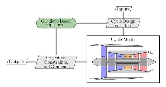
The overall structure of the pyCycle code is presented as an extended design structure matrix (XDSM) diagram [36] in Figure 2. Many elements in this diagram are likely recognizable by cycle analysts familiar with modular tools such as NPSS. There are four primary computational parts to a pyCycle model which appear along the diagonal: Optimizer, Solver, Cycle, and Balance. These four parts do not work in isolation, but pass data as indicated by the gray lines with the type of data passed between the parts specified in the gray parallelograms. Finally, the white parallelograms indicate inputs and outputs from the code.
From the thermodynamic cycle analysis perspective, the Cycle block is the heart of the code as it contains all of the governing thermodynamic equations needed to model an engine. While this is shown as a single block in the figure, it is actually a set of modular cycle elements such as compressors, burners, or turbines which can be combined to model almost any arbitrary engine design. The calculations executed in the Cycle block do not explicitly result in a valid model as there are physical dependencies and design rules which must be satisfied. These physical dependencies and design rules are captured in the Balance block as a set of implicit state variables and associated nonlinear residual equations that are converged by the Solver. (In NPSS, implicit state variables are called “independent variables” and residual equations are called “dependent equations”, but pyCycle adopts the terminology used in the MDO field.) Lastly, there is the Optimizer, which finds the design variable values that satisfy the constraints and minimizes the objective specified for the problem.
Developing these four blocks and combining them into a complete cycle analysis and optimization tool involves the challenge of combining thermodynamic analysis, software engineering, numerical methods, and optimization techniques. For pyCycle, this challenge was made easier by developing the code on top of NASA’s OpenMDAO framework [31], using the framework as the bottom layer in pyCycle’s software stack. OpenMDAO was selected as the basis for pyCycle for a number of reasons. First, OpenMDAO provides the required modular, object-oriented modeling structure comprised of explicit and implicit calculation objects (components). Components provide the foundation for creating the thermodynamic cycle calculation and balance blocks shown in Figure 2. Second, in keeping with the modularity theme, OpenMDAO provides a modular optimizer and nonlinear solver implementation allowing for a variety of methods to be used in those parts of the code. Third, OpenMDAO provides functionality for automatically computing derivatives across large, complex models for use with efficient gradient based optimization techniques. In combination, these three characteristics facilitated the development of pyCycle to satisfy the primary research objective of creating a modular cycle analysis tool suitable for integration into a multidisciplinary aircraft design optimization process. The following sections provide relevant details on the major features of pyCycle with an emphasis on the differences with respect to other state of the art cycle analysis tools such as NPSS.
2.1. Analysis, Optimization, and Analytic Derivatives
The first pyCycle blocks presented are those related to the Solver and Optimizer blocks shown in Figure 2. While these blocks do not contain calculations unique to cycle analysis, they play an important role in shaping the overall computational process for the code. Furthermore, the objective of the pyCycle code development was to improve cycle analysis for unconventional engine architectures by implementing advanced mathematical methods in these two blocks, specifically in regards to calculating gradients. Therefore, the Solver and Optimizer blocks play a central role in enabling the desired pyCycle capabilities.
The propulsion cycle design problem in Table 1 presents a formal mathematical description of the complete optimization problem to be addressed by pyCycle. In this problem statement, the goal is to minimize an objective function (f) by changing the design (x) and state variables () while considering both equality and inequality constraints (, , , and ). The role of the optimizers and solvers in the cycle analysis code is to identify the best solution which satisfies the given requirements and constraints. In theory, this entire problem could be handled using only an optimizer by giving it responsibility for minimizing the objective function as well as satisfying all the constraints by controlling both the design and state variable values. While this approach eliminates the need for the solver, it necessitates that the optimizer navigate a larger design space while also satisfying a large set of equality constraints. Practically speaking, the optimizer-only approach is never used, but it does provide a useful way to understand how the more common solver-based approach changes the computational requirements of the problem in the context of an optimization. Using a solver to converge the equality constraints creates a reduced-space form that presents a smaller number of design variables and constraints to the optimizer. The task of converging the reduced space problem is what is commonly referred to as a cycle analysis.
The cycle analysis problem, given in Table 2, finds the state variable values (y) which make the residual equations () true given values for the design variables (x). The residual equations and state variables in this reduced-space problem are comprised of the physical governing equations (), the conservation laws (), and the design rules () described in Table 1. The three sets of implicit variables () and associated residuals are aggregated together for convenience and compact notation.
The residual equations, , form a system of nonlinear equations which are converged through the use of a numerical solver, typically based on Newton’s method. Newton’s method iteratively converges to a solution by starting with an initial guess of the state variable values in the neighborhood of the solution. From this initial guess, improved values for the state variables are obtained through successive applications of Equation (1) where the subscripts m and refer to the current iteration and next iteration values for the state variables, respectively. Of note in this equation is the need for partial derivatives of the residual values with respect to the state variables. The computation of these partial derivatives can be accomplished by several means. NPSS uses finite-difference approximations to compute , while uses pyCycle hand differentiated analytic partial derivatives.
An optimization problem can then be wrapped around the cycle analysis, creating a so-called reduced space formulation because of the smaller set of design variables and constraints that the optimizer is presented with. The reduced-space optimization problem is given in Table 3. This problem minimizes the objective function (f) by altering the design variables (x) while satisfying a set of design limits posed as inequality constraints (). While a wide array of optimization algorithms can be applied to solve to this problem, pyCycle development focused on enabling the use of gradient based techniques for their significant computational efficiency. The sequential quadratic programming algorithm implemented by the SNOPT [37] library was selected as the optimizer for the work presented in this paper, although pyCycle will work with any gradient based algorithm.
If cycle analysis solutions are all that are desired, then Table 2 and Equation (1) are all that are required. However, to wrap a gradient based optimization algorithm around a cycle analysis, additional calculations of total derivatives (i.e., and ) are required. While these derivatives initially only appear to be dependent on the design variables (x), it must be recognized that altering these values also requires a reconvergence of the implicit state variables (y) by the nonlinear solver. Therefore, the total derivatives calculations must include the effect of changes in y as a function of changes in x. Using as an example, applying the chain rule results in the total derivative definition given in Equation (2).
The partial derivatives terms in Equation (2) ( and ) are relatively easy to compute through a variety of techniques that will be discussed later in this section. However, the total derivative term in Equation (2) () presents a much larger computational challenge. This term captures the change in the converged state variable values with respect to changes in the design variables. Computing this term directly requires reconverging the full system of nonlinear equations once for each individual variable in y. Additionally, the accuracy of such an approach may be limited due to the solver tolerances used in this reconvergence process. However, this total derivative can be more efficiently computed using an indirect approach that requires only partial derivatives of the residual equations . This approach again applies the chain rule as given in Equation (3). In this equation, it is assumed that the total derivatives are taken around a converged point for any x, thereby also specifying that .
Equation (3) can be rearranged to compute as a function of only the partial derivatives of the residual equations as given in Equation (4). Used together, Equations (2) and (4) form what is referred to as the direct analytic method for computing total derivatives. The direct analytic method requires only the use of partial derivatives and the solution to a linear system (Equation (4)), which must be solved once for each design variable in x. Therefore, its computational cost scales linearly with the number of design variables (and independent of the number of constraints) making it very efficient for optimizations involving a relatively small number of design variables.
However, most multidisciplinary propulsion system design optimization problems consider a relatively large set of design variables, with number of variables significantly exceeding the number of objectives and constraints. In this situation, the derivative equations can be manipulated to form the adjoint analytic method as shown in Equations (5) and (6). The adjoint method includes a linear system, which must be solved once for each objective and constraint in the optimization problem (i.e., f and from Table 3). As a result, the adjoint method’s computational cost scales linearly with the number of constraints in the optimization problem and is independent of the number of design variables making it more computationally efficient in many cases. In practice, optimizations for large vehicle level models that include many disciplines and higher order models almost always have many more design variables than objectives and constraints, thus the adjoint method is more commonly used.
Regardless of which of the two analytic techniques is applied, computing the total derivatives first requires finding partial derivatives of the objective function, residuals and constraints with respect to both the design and state variables. Similarly, applying Newton’s method to solve the system of nonlinear equations requires computation of the residual equation partial derivatives with respect to the state variables. It is therefore clear that accurately and efficiently computing these partial derivatives throughout the system is critical to the overall success of the optimizer and solver algorithms.
In OpenMDAO and by extension pyCycle, several options are available for computing the partial derivatives throughout a model. The first option is to use finite difference approximation. While this option is easy to implement, the method can be computationally expensive for large numbers of design and residual variables and suffers from numerical accuracy issues. However, it must be noted that the finite differences in this case are taken only across the residual evaluations and hence are far more accurate than if a monolithic finite difference was taken across the full nonlinear analysis. A second option is to compute the partial derivatives using the complex step approximation method [38]. This method provides more accuracy than finite differencing but it is also more computationally expensive and requires the code inherently handle complex computation—although many pure Python analyses do inherently handle this correctly. The third option is to compute the partial derivatives analytically via symbolic, algorithmic, or hand differentiation of the equations throughout the code. While more challenging to implement in the code, the third option provides precise partial derivative values that are both computationally efficient completely accurate. As a result of these benefits, analytic computation of partial derivatives (specifically using hand differentiation) was the approach implemented in pyCycle and represents a fundamental advancement in cycle analysis capability contributed by this research.
Using hand differentiation for a modular cycle analysis code requires special consideration in regards to structuring the code base. Specifically, the code for the various modular engine components needs to be written to not only provide functional outputs, but also the partial derivatives for all the outputs or residual values with respect to any input or implicit state variable. With each modular element providing its own partial derivatives, the required overall partial, and ultimately the total derivatives, across any combination of the cycle elements must then be computed. OpenMDAO, and by extension pyCycle, facilitates this process by automatically applying the direct or adjoint analytic methods for any given model. This automatic total derivative calculation enabled the formulation of a modular cycle analysis code and guided the decisions about how to decompose the various cycle analysis calculations described in the next section.
2.2. Physical Equations of Cycle Analysis
The solver, optimizer, and derivative calculations methods described in the previous section are general mathematical approaches which can be applied to determine the solutions of a wide variety of reduced-space optimization problems. For the development of pyCycle the reduced-space problem is formed via the combination of the Cycle and Balance blocks, and of those two the actual governing equations and engineering calculations are contained within the Cycle block. This section describes how the physical equations of cycle analysis were implemented to construct the Cycle block in a modular fashion that met the requirements for pyCycle.
Generally, the cycle analysis of a gas turbine engines seeks to compute the overall performance characteristics by determining changes in thermodynamic properties of gases as they move through the engine. These changes in the thermodynamic properties are imparted by the various components of the engine such as a compressor or combustor. For modular codes such as NPSS and pyCycle, these physical engine components are modeled as individual “elements” which can be stitched together to form a model for a specific engine architecture. Internal to each of the cycle objects, an number of calculations are completed which generally fall into two categories: thermodynamic properties calculations (i.e., chemical equilibrium) and engineering calculations. In NPSS, the individual cycle elements such as compressors or combustors are the atomic computational objects in the model—the lowest level objects the software recognizes—and contain both types of calculations. In contrast, pyCycle elements are themselves composed of several nested layers of smaller computational components that capture the different types of calculations. Although pyCycle users will still build models by stitching together cycle element objects, the finer grained internal decomposition of the elements is an important distinction necessitated by the need to provide analytic partial derivatives. By sub-dividing the elements into smaller computational sub-components, hand differentiation of the various partial derivative terms was made significantly simpler. The automatic total derivative functionality of the OpenMDAO framework is then relied on to combine these simpler partial derivatives together to obtain the derivatives for the overall elements and cycle model. Typical users of pyCycle will be able to use a standard library of pre-defined elements (e.g., inlet, nozzle, compressor, and turbine) which already have analytic derivatives implemented, but when new elements are coded for a specific model users would need to provide derivatives for the new code.
Before providing an example of this sub-divided element structure, it is first important to describe a critical sub-element in pyCycle which differs in implementation from NPSS: the thermodynamic property calculation sub-element. In NPSS, the calculation of thermodynamic properties is completed by a “Flowstation” object, with the calculation method internal to this object selected by the user (either GasTbl, AllFuel, Janaf or CEA). While some of methods are simply table lookups, others (specifically Janaf and CEA) perform a chemical equilibrium convergence that uses a set of physical residual equations and a nonlinear Newton solver. These residual equations and the associated solver are hidden within this object forming a nested solver structure. Nesting these residual equations and the solver inside the Flowstation object is advantageous for NPSS as it produces a separate, smaller nonlinear systems of equation which can more easily be finite-differenced and converged. However, the nested nonlinear solver approach of NPSS poses a challenge for the computation of analytic derivatives because it requires the nested application of the direct or adjoint derivative calculation methods.
For pyCycle, the thermodynamic properties are computed using a minimization of Gibbs free energy approach very similar to that of Gordon and McBride [30] and consistent with the CEA option in NPSS. Some minor modifications were made to the numerical solution methods of this approach to facilitate computation of analytic derivatives and are documented in prior work by the Gray et al. [32]. In comparison to the NPSS implementation of this method, however, pyCycle uses a flattened formulation that exposes all of the chemical equilibrium and thermodynamic residuals to the top-level solver. This flattened approach results in a larger system of nonlinear equations for the top-level solver but simplifies the task of computing analytic derivatives. Therefore, pyCycle models have one to two orders of magnitude more physical residual equations in the top-level solver compared to an equivalent NPSS model: for pyCycle compared to for NPSS. This change to the approach for solving the chemical equilibrium residual equations represents a significant change in model structure necessitated by applying analytic derivatives methods to cycle analysis.
To help describe the internal decomposition of pyCycle elements, an example of the sub-element structure and calculations for a simple compressor is shown in the XDSM diagram in Figure 3. In this figure, inputs to the calculations, either from upstream components or user specification, are given in the white parallelograms at the top with outputs of the element shown in the white parallelograms on the left. Overall, the calculations required to model this simple compressor are decomposed into six sub-blocks. In this figure, the total and static thermodynamic calculations are shown in blue with engineering calculations in red. The first sub-block, Pressure Rise, computes the compressor exit pressure () based on an input pressure ratio (PR) and entrance pressure (). The calculation and the associate partial derivatives for this component are given in Equation (7).
Next is a thermodynamic solution that computes the ideal thermodynamic properties at the compressor exit (isentropic pressure rise), specifically the ideal exit enthalpy (). This value is combined with the compressor entrance enthalpy () and input efficiency () to compute the real—as opposed to ideal—exit total enthalpy () in the Enthalpy Rise sub-block. The equations and associated partial derivatives for this calculation are given in Equation (8).
The computed exit total enthalpy and pressure are then used as inputs to a thermodynamic solver sub-block that calculates the complete set of real total thermodynamic properties at the compressor exit. Following the determination of the real flow properties, the Power sub-block computes the power () and torque () required from the shaft to drive the compressor. This sub-block takes entrance and real exit enthalpies as inputs along with the compressor mass flow () and shaft speed (N). Calculation of the required power and torque along with their derivatives is completed following Equations (9) and (10), respectively.
Lastly, the final sub-block of the compressor element computes the real static thermodynamic properties, based on the real exit total properties and a specified exit Mach number. Together, these six blocks of code compute effect of the thermodynamic process of a compressor and provide the partial derivatives OpenMDAO needs to compute analytic derivatives for an optimizer using the direct or adjoint method.
In summary, this example for a simple compressor provides an overview of how pyCycle elements are constructed from smaller sub-blocks along with how the functional and derivative calculations performed by each sub-block of code. Similar diagrams describing the decomposition of other simple engine elements can be found in a paper by Hearn [39]. Although this simple compressor demonstration required just six sub-blocks, the actual elements implemented in pyCycle are much more complex. For example, the full compressor and turbine elements contain additional code to account for the performance maps that provide efficiency. Other elements also include sub-blocks that account for the impact of bleed extraction, cooling flows, and heat transfer. Details of the calculations for every element are not necessary to understand how pyCycle is implemented, since all elements follow the blue-print laid out in the example compressor above. Further details on each element are available in the pyCycle source code.
2.3. Implicit Relationships with the Balance Block
While the Cycle block computes the flow properties and performance characteristics of individual engine elements, simply coupling these elements together to make an engine model does not result in a physically valid or desirable design. In addition to the governing equations there are additional engine level conservation equations and design requirements that must be satisfied. The Balance block, shown in Figure 2, handles these engine level residual equations (in NPSS these are called “dependents”). Associated with these residual equations are a set of implicit state variables (in NPSS these are called “independents”) whose values are found by the nonlinear solver such that the residuals are driven to zero. In Table 1, the residual equations associated with the Balance block were labeled as and . The specific residual equations required for any single cycle analysis are highly dependent on the system being modeled, the intentions of the user, and whether the model being executed in design mode or off-design mode. Thus, while the details of the nonlinear solution process were provided in Section 2.1, this section goes into more detail about the specific residuals that are needed for different models.
The physical residuals, , are those required for cycle matching; they ensure that the physical conservation laws are respected. In NPSS, these equations, and the associated state variables, are often hidden from the user by an automatic configuration routine. In pyCycle, there is no automatic configuration of the cycle matching residuals and the user must always configure them. Equations (11) and (12) below give examples of engine matching residual equations typically used in a gas turbine cycle model. First, from the conservation of energy, the net torque on any shaft (the sum of the torques from the compressor and turbine) must be zero as defined in Equation (11). To satisfy this equation, a state variable is typically created for the turbine pressure ratio (design mode) or the shaft speed (off-design mode). The second example in Equation (12) comes from off-design compressor calculations where the actual corrected mass-flow through the compressor must match the allowable value specified in the compressor performance map based on the corrected speed and operating characteristic (known as its R-line). In this residual equation, the corrected flow computed from the performance map must equal the corrected flow being passed into the compressor. To satisfy this equation, the compressor map R-line value is typically included as a state variable in the nonlinear solver. These two examples provide an illustration of how physical conservation laws are implemented through implicit residual relationships used to ensure conservation of mass, momentum, and energy at the 1D thermodynamic level. Both pyCycle and NPSS implement these physical relationships following this approach and converge them with them with a Newton solver.
In addition to the physical conservation residuals, cycle models also commonly contain a set of design rules as residual equations () which guide the cycle analysis. These design rules are implemented to capture design intent and operating philosophy for the engine and are therefore highly model specific. For example, Equation (13) might be implemented by the user to ensure that the net thrust produced by the engine matches a specified target thrust. The state variable added to the analysis along with this residual equation is also model dependent. In this case, one likely state variable would be the overall engine mass flow rate as it has a direct relationship with the amount of thrust that can be produced by a given Brayton cycle. Similarly, Equation (14) could be used to drive the combustor exit temperature () to a target value at a certain flight condition. The associated state variable controlled by the solver for this residual again depends on the design and operating philosophy selected, but a common selection would be the fuel-to-air ratio of the combustor.
Overall, the Balance block within the code contains a vital set of residual equations for both physical conservation laws and design rules which govern the thermodynamic cycle analysis. These equations must be uniquely defined for each engine model depending architecture being studied on the design principles being applied. The next section presents the development of a specific thermodynamic cycle model, including the appropriate residual equations, which is used throughout the remainder of this paper for verification, derivatives comparisons and evaluation of the pyCycle in an optimization problem.
3. Example Problem
To evaluate the features of pyCycle relative to the present state of the art, a reference engine model was constructed in pyCycle as well as NPSS. The NASA advanced technology high bypass geared turbofan engine cycle [40], referred to as the “N+3” engine, was selected for this research and was modeled in both tools, with the outputs compared in detail to ensure that both compute the same engine cycle performance. The N+3 reference cycle represents a notional high bypass ratio geared turbofan that could be available in the 2030–2040 time frame. The cycle includes several advanced features to improve its overall performance. These features include a low pressure ratio fan to enable a high bypass ratio, which also requires a variable area fan nozzle to maintain the fan stability throughout the flight envelope. Furthermore, the baseline design has an overall pressure ratio around 55, with a maximum allowable combustor exit temperature of 3400 R, and an uncooled low pressure turbine. This advanced cycle is modeled with a fairly complex, multi-design point (MDP) process that involves simultaneous consideration of performance at four different flight conditions. The complexity of this model makes it well suited for use in verifying pyCycle against NPSS using comparable models built with the two cycle modeling libraries. This section describes MDP model structure, starting with the basic formulation used to capture performance at any single flight condition, then describes how multiple operating points are integrated together to for the MDP analysis. This description provides an overview with sufficient detail to understand what is being modeled and the level of detail to which the verification between the two codes was performed.
3.1. Modeling a Single Flight Condition
As described above, cycle models in pyCycle are built up by linking a set of modular cycle elements together to represent the full propulsion system. For the N+3 geared turbofan cycle, twenty-five elements are connected together, as shown in Figure 4. In this figure, the blue arrows indicate flow connections between elements and ultimately define the flow-path. Following the arrows illustrates that the engine cycle model has two separate streams, terminating in two nozzles: Fan Nozzle and Nozzle. The red lines indicate physical shaft connections to the three shafts (often referred to as spools): HP Shaft, LP Shaft, and Fan Shaft. Lastly, the green lines indicate secondary data connections between elements. These connections do not represent any physical aspect of the engine, but rather provide necessary information for elements to perform their calculations. For example, the Fan Nozzle and Nozzle elements need to know static pressure from the Ambient element in order to compute the correct gross thrust. Similarly, the Performance element needs to know the ram drag from Inlet and the gross thrust from both Fan Nozzle and Nozzle in order to compute net thrust.
To predict the cycle performance at any single flight condition, the model represented in Figure 4 needs to be executed in two different modes, with the outputs from each combining to provide a full description of the performance characteristics of the engine. These two modes are referred to as “on-design” and “off-design” by the cycle analysis community. The fundamental model structure (the elements and their connections to each other) remain identical in both modes, but the internal calculations within each element vary slightly and consequently the conservation equations () and design rules () also change.
In the context of using a cycle model as part of a design optimization, or even just as part of a larger overall vehicle system model, the terms “on-design” and “off-design” are potentially confusing and warrant further clarification. The on-design mode is computed around a reference flight condition, usually sea-level-static (SLS) or top-of-climb (TOC), where it is desirable to specify key cycle design parameters such as compressor pressure ratios, combustor temperatures, and shaft speeds. For the N+3 engine, TOC (MN: 0.85, altitude: 35,000 ft) was selected as the reference on-design condition. Given the specific set of design parameters, the on-design mode calculations will compute a set of physical design values such as flow areas and compressor and turbine map scalars that will be constant for the cycle at all other operating conditions. These physical constants () are required inputs for the off-design calculations. The on-design mode set up for the N+3 cycle model is shown in Figure 5. The residuals provided by the Balance block include both and sub-sets.
There is one set of conservation residuals (), one for each of the three shafts, that ensures the net torque on each shaft is zero, producing steady state operation as given in Equation (15). The associated state variables for these residuals are the turbine pressure ratios on each shaft, and , as well as the gearbox output torque to the fan shaft.
The remaining residuals from the Balance block in Figure 5 are part of the design rules for this engine and are given in Equation (16). Equation (16) drives the cycle to match the specified design targets for and . The associated degrees of freedom for these residuals are the combustor fuel-to-air ratio () and high pressure compressor pressure ratio (). It also includes one residual equation per compressor and turbine that is used to enforce a technology assumption for turbomachinery polytropic efficiency (). This implicit relationship is needed because the Compressor and Turbine elements take adiabatic efficiency () as an input, and output a computed polytropic efficiency. The solver finds the adiabatic efficiency as a state variable such that the target polytropic value is achieved.
As shown in Figure 5, the on-design calculations produce outputs including thrust specific fuel consumption (TSFC) and . While these outputs are metrics for evaluating performance at the design condition, the on-design calculation’s most significant outputs are the physical design parameters . These parameters specify the engine design characteristics which are constant across all operating conditions. The specific variables that are included in depend on the particular engine cycle model that is constructed. Generally, the list includes the physical flow areas throughout the engine as well as tubomachinery map scalers for Compressor and Turbine elements.
The off-design mode calculations are responsible for determining performance of the propulsion cycle model at all flight conditions of interest. As stated above, the off-design mode shares an identical model structure to the on-design mode calculations but has different input parameters and residual equations. Figure 6 shows the XDSM diagram for the off-design model calculations of the N+3 cycle model considered in this work. The set of physical residuals applied in the N+3 off-design model are given in Equation (17). In Equation (17), the residual for is the same as for the on-design mode; it enforces that there is zero net torque on the shaft to respect conservation of energy. The residual related to the nozzle throat area, , enforces conservation of mass by ensuring that the mass-flow through the cycle is enough such that the flow area required equals the physical area of the nozzle throat. The state variables for these physical residuals are the shafts speeds (, and ), and engine mass flow rate ().
The remaining residuals are associated with design rules as given in Equation (18). The first residual in Equation (18) regulates the fan-stall margin, which is primarily achieved by varying the bypass ratio () as an implicit state. The net thrust residual provides a throttle setting for the engine, and is mainly regulated by . The cooling mass flow residual set, one for each cooling flow in the engine, matches the cooling mass-flow rate (), to a prescribed value. As discussed in more detail in the next section, the cooling flow for this cycle is defined by the cooling needs at the rolling takeoff flight condition, and at all other conditions it is given as a prescribed input. In addition to these residuals, the outputs from the off-design analysis of the reference engine are the net thrust and the TSFC.
3.2. Multi-Design Point Modeling
The on-design and off-design analysis modes described in the previous section are traditionally used in a sequential process to evaluate the performance of a gas turbine engine. First, the on-design analysis is completed to develop the cycle design that satisfies the performance requirements at a single operating condition. Once this is completed, the off-design analysis mode is used to evaluate the performance throughout the remainder of the flight envelope to ensure operating requirements are satisfied. If the performance characteristics determined in the off-design mode are not satisfied, a manual iteration is then undertaken to modify design inputs and reevaluate the cycle in both on- and off-design modes. This traditional process works well for relatively simple engine designs with a limited set of performance requirements at off-design operating conditions.
However, as the engine concepts being evaluated become more complex with performance requirements and constraints at multiple flight conditions, applying this traditional manual approach becomes more difficult. In these situations, a more advanced cycle modeling technique known as multi-design point (MDP) [41] can be used. The MDP method uses the same on-design and off-design analyses described above, but combines them to simultaneously evaluate performance at multiple operating conditions and automatically use that information to develop a feasible design. Essentially, the method creates on-design and off-design instances of the model which are then coupled together and simultaneously executed. This coupling commonly includes passing of design variables () as well as an additional Balance block. The states and residuals associated with this Balance are selected to ensure a design is generated that satisfies the various requirements and constraints at each critical operating point. Again, it should be noted that the terms “on-design” and “off-design” are potentially confusing. Recall that these terms refer to the computational mode of cycle analysis points. Despite the confusing terminology, in an MDP, all of the cycle analysis points can be considered design-conditions for the engine cycle.
In the original study on the N+3 engine model, Jones used a four-point MDP model to size the advanced high-bypass ratio turbofan [40]. The four points include top-of-climb (TOC), rolling takeoff (RTO), sea-level static (SLS) and cruise (CRZ), and their organization into an MDP model is shown in Figure 7. The TOC design point was instantiated as an on-design model, and was built following the configuration in Figure 5. The other design points (SLS, RTO, and CRZ) were set up as off-design models following the configuration in Figure 6.
Figure 7 shows two sources of coupling at the MDP level in addition to the design variables. The first coupling results from the calculation of cooling flow requirements which are determined at the RTO design point as this flight typically experiences the highest gas temperatures. The cooling mass flow rates () are output by the RTO and create a cyclic data connection with the TOC block that proceeds it. Second, the Balance block adds a set of additional design rule residual equations that implicitly relate the performance of different operating conditions to each other. These design rules set a jet velocity ratio at cruise (), set the maximum combustor exit temperature at RTO () and define the relative combustor temperatures between TOC and RTO. In addition, the design rules specify the relative net thrust produced by the engine between several different design points. To satisfy these design rules, the solver is given control of five state variables including the TOC mass flow rate (), TOC bypass ratio (), TOC combustor exit temperature (), SLS net thrust () and CRZ net thrust ().
As shown in Figure 7, the MDP formulation for a cycle model is significantly more complex than a traditional single-point design, but that complexity comes with the benefit of a significantly more well-defined propulsion design specification. Using an MDP formulation ensures that the cycle performance matches well with the aircraft requirements for any given combination of design variables, making the optimizer’s job easier. The MDP model of the N+3 reference engine is used throughout the remainder of this paper to verify and evaluate pyCycle.
4. pyCycle Verification
The first step in evaluating the pyCycle code was to verify that the code properly performs the thermodynamic cycle analysis calculations. For this verification, the MDP N + 3 engine model described in the previous section was evaluated using the baseline design specified by Jones. This verification therefore did not include the Optimizer but instead focused on ensuring the Solver, Cycle, and Balance are implemented correctly.
The first portion of the verification study focused on examining the thermodynamic properties computed by pyCycle throughout the N + 3 engine model. It is important to first note that the core thermodynamic property solver of pyCycle was previously verified by Gray et al. [32] via extensive comparisons to the CEA tool. The present study differs from that verification in that it examined the properties determined by a fully converged engine model and therefore verifies the engineering calculations present in each of the cycle elements and balance residual equations. Figure 8 shows the relative difference in the thermodynamic property outputs at the exit of each component in the engine for each of the four design points. As shown in this figure, the maximum relative difference for any thermodynamic property was approximately 0.03% indicating excellent agreement.
In addition to examining thermodynamic properties at each flow station, the overall performance metrics calculated by the pyCycle and NPSS models were also compared. Table 4 shows the NPSS and pyCycle performance values along with the relative difference at each of the four design points included in the model. Again, the relative difference for these outputs was very small with most values less than 0.02%. The one exception was the SLS ram drag, which had a relative difference of approximately 0.15%. This larger difference shows that there are some minor differences between the codes when evaluating static thermodynamic properties at very low Mach number flows (in this case, Mach 0.001 from the SLS point). While larger than the other differences reported in Figure 8 and Table 4, this difference was ultimately determined to be acceptable given the low Mach number flight condition.
Overall, the thermodynamic and performance comparisons described in this section found relative differences between pyCycle and NPSS outputs to be below 0.03% for most outputs. This level of difference provides strong evidence to verify that pyCycle components and overall engine models properly model thermodynamic cycles. Additional efforts may be made in the future to further reduce this difference, particularly for low Mach number flow conditions. However, there is a practical limit to the level of difference achievable as the presence of solvers with convergence tolerances in each code naturally introduces error into cycle model outputs. Given these results and limitations, the pyCycle code was deemed sufficiently verified against the current state of the art code NPSS to proceed with evaluating the analytic derivative calculations and the use of pyCycle for design optimization. A complete output from this verification study is provided in Appendix A.
5. pyCycle and NPSS Derivative Comparison
The previous section provided the results of a detailed study to verify that pyCycle was capable of producing results in agreement with the NPSS analysis tool. While this verification step was important to the development of pyCycle, the primary motivation for creating this code was to support gradient-based optimization of a thermodynamic cycle model in the context of a larger vehicle system design. In this context, the accurate computation of total derivatives across an engine model is required to provide the gradient information needed to direct the optimization algorithm. This section examines the total derivative calculation, described by Equations (2) and (4), required for this type of optimization for the N + 3 Reference Engine. This examination was completed by implementing three different derivative calculation approaches, which were applied to both pyCycle and NPSS, respectively, and comparing the resulting computed values.
The first approach considered in this evaluation was to compute the total derivatives required for optimization using the analytic derivatives defined in pyCycle. These derivatives were computed by first hand differentiating the thermodynamic equations required for each of the code elements (described in Section 2.2 and Section 2.3) to get the partial derivatives. The total derivatives were then computed using OpenMDAO’s automatic implementation of the direct and adjoint analytic derivative equations. The hand differentiated partial derivatives used in this process were thoroughly checked and verified for each element using finite difference or complex step approaches. Therefore, for the results presented in this section, the analytic derivatives were considered to be the accurate total derivatives to reference from.
The second approach considered for computing total derivatives in this study applied a monolithic technique that would be typically applied in determining total derivatives with existing cycle codes such as NPSS. In this approach, the entire cycle analysis code is treated as single, black box object without any knowledge of the internal calculations. The Solver, Cycle and Balance objects shown in Figure 2 are hidden inside this box with only the inputs and outputs available. With this setup, the total derivatives can be calculated through finite difference approximation by systematically varying the input variables and recording the changes to the output values.
This total derivative calculation process is straightforward and is easy to apply to existing cycle analysis codes such as NPSS. However, computing derivatives with this process presents a number of opportunities for the introduction of error into the derivative calculation and is computationally intensive. First, the monolithic approach treats the code inside the black box as an explicit calculation with outputs directly dependent on the inputs. However, the internal calculations for cycle analysis include converging a set of nonlinear residual equations within a defined tolerance. This numerical convergence process therefore produces output values that are not exact (due to the tolerance on the residual equation convergence) and instead include some level of error (). These errors in the functional evaluation alter the derivative approximation, as shown in Equation (19). This error can often be minimized by tightening the solver tolerance inside the monolithic code with the downside of increasing computational time required to converge the model. However, the error introduced by the presence of the internal solver can never be fully eliminated and its impact on the derivative values can be difficult to quantify.
The other source of error for the monolithic derivative calculation approach is the need to take a finite step size in the computation process. For nonlinear equations, smaller step sizes should theoretically lead to more accurate derivative approximations. However, there is a practical lower limit for the step size as subtractive cancellation will occur as result of numerical precision limits [38]. Computing derivatives with small step sizes is further complicated by the presence of internal solvers in the monolithic approach. If the step size is too small, the change in input might not be sufficient to increase the residual values above the specified tolerance. As a result, the step will produce no change in the output values as the numerical solver does not have to reconverge to produce “valid” output. In this case, the derivatives computed by the finite differences will be zero. These issues with the monolithic approach around NPSS models with internal solvers are further described in the work of Hendricks [4].
The last approach considered in this study for computing total derivatives applied a semi-analytic method. This approach can be considered an intermediate approach between the monolithic and analytic approaches described above. In this approach, the derivatives are computed using the direct—Equations (2) and (4)—or adjoint—Equations (5) and (6)—analytic methods. However, the partial derivatives needed to apply the analytic methods were computed using finite differences rather than hand differentiation. While this approach still uses the finite difference method, the calculation process is significantly different than the monolithic approach because it does not require the internal code solver to reconverge as part of finite differences. Instead of reconverging the solver, the process executes a single pass through the model to compute the partial derivatives of the outputs and residual equations (i.e., dependents in NPSS) as a function of both the inputs and implicit state variables (i.e., independents in NPSS). The approach thereby increases the total number of finite difference calculations which must be completed but eliminates the need for the internal solver during these calculations and dramatically reduces the cost of each finite difference computation. As this approach does eliminate the need to reconverge the residual equations within the finite difference calculation, it eliminates the solver tolerance issues described for the monolithic approach. Regardless, finite difference approximations are still present and therefore the semi-analytic method still suffers from the limitations associated with subtractive cancellation with small step sizes.
The three methods described above were implemented in this study for the N + 3 reference engine to examine the total derivative values they compute and their impact on gradient based optimization. The analytic approach was implemented using pyCycle, with the monolithic and semi-analytic approaches implemented using NPSS. Figure 9 shows the total derivatives of net thrust at two design points (TOC and CRZ) with respect to the top-of-climb and rolling takeoff . The derivatives for the thrust at the other two operating points (SLS and RTO) are not shown as they are fixed inputs to the model. Furthermore, the total derivatives for TSFC at each of the four design points with respect to the same inputs are shown in Figure 10. In these figures, the plots depict the error between the derivative values computed by the monolithic approach and semi-analytic approaches relative to the fully analytic approach. For the monolithic approach, three different internal solver tolerances were evaluated and are represented by the orange, green and red lines. For each of these monolithic approaches and the semi-analytic approach (shown in blue), a range of relative step sizes was also evaluated to show the effect of this value on the computed derivatives.
Examination of the total derivative errors for the monolithic and semi-analytic methods in both these figures reveals several important insights. First and most generally, the figures show that the accuracy of the total derivatives computed with these approaches vary substantially depending on the derivative being computed, the relative step size, and the internal solver tolerance. This variability makes it difficult to select values for step size and tolerance for total derivative calculation as the best choice is not known a priori. For the sake of simplicity, a single step size is often used for all inputs, but these results show that this can lead to large errors in some derivatives even if others are approximated accurately. Second, for the semi-analytic approach, the general trends show that smaller step sizes typically result in more accurate total derivatives. At the smallest step size, the errors for the total derivatives were found to be on the order of 1%. This result is consistent with the definition of the derivative which states that derivative gets more accurate as the step size approaches zero. Furthermore, the results show that the step sizes taken in this study, while being small, do not approach the practical limit resulting from subtractive cancellation. Lastly, the total derivative plots show significant variation and limitations for using the monolithic approach with finite difference approximation. For the largest internal solver tolerance of 10−4, the accuracy of the derivative decrease as the step size decreases, reaching 100% error at step sizes below 10−4. This level of error occurs as a result of the specified step size not being large enough to cause the solver to become unconverged. As a result, the functional value is the same with and without the step (i.e., ) producing a total derivative of zero and 100% error. A similar outcome is also visible for the intermediate monolithic tolerance at tolerance and step sizes of 10−6. While 100% error is observed at this combination, at larger step sizes for the same tolerance, there is again significant variation in the accuracy of the total derivative computed. The error in these derivative computations is typically between 1% and 10% with the value depending on both the step size and total derivative being computed. Slightly better total derivative accuracy can generally be achieved using monolithic approach with a 10−8 solver tolerance. However, this approach typically still had errors on the order of 1%, indicating a practical limit for the accuracy that can be achieved by finite differencing monolithic codes even with tightly converged internal solvers.
In addition to accurately computing total derivatives, the analytic method implemented in pyCycle provides a significant improvement in the computational speed for obtaining these values. To evaluate the computational performance, total derivatives were computed with pyCycle and several different combinations of step sizes and solver tolerances for the monolithic and semi-analytic approaches implemented with NPSS. The total derivatives evaluated were those for net thrust, TSFC and fan diameter with respect to ,, , , , and . Table 5 lists the time required to compute these derivatives with each of the different methods. As shown in the table, computing the total derivatives with pyCycle is extremely efficient and can be done in just under 2 s. By comparison, the fastest semi-analytic approach takes over 20 min while the best monolithic approach takes over 30 min. This disparity shows the significant computational benefits that can be achieved through the use of analytic derivatives over traditional approaches for computing derivatives for existing codes such as NPSS.
In summary, this section shows the accuracy and computational efficiency of several different approaches for computing total derivatives across thermodynamic cycle models. The fully analytic approach was implemented by pyCycle while the semi-analytic and monolithic approaches were implemented with NPSS. The total derivatives for net thrust and TSFC computed by these three methods were evaluated for the N + 3 model with errors computed relative to the analytic approach. The semi-analytic and monolithic approaches both produced inaccurate total derivatives, with the errors found to be a function of the step size, solver tolerance and the derivative being evaluated. Furthermore, the monolithic and semi-analytic approaches required several orders of magnitude more time for calculation to generate these inaccurate derivative values. With these differences in accuracy and computational cost, the question remains: How do the different approaches for computing derivatives impact the gradient-based optimization of a thermodynamic cycle? This question is examined using the N + 3 reference engine in the next section.
6. pyCycle and NPSS Optimization Comparison
pyCycle was developed with analytic derivatives to support the use of gradient-based optimization on problems using larger vehicle system models that included thermodynamic cycle analysis. To evaluate this capability relative to the current state of the art, an optimization study was completed for using the MDP N + 3 reference engine described in the previous sections. The original report by Jones [40] describing this engine showed a trade space around the selected baseline design in terms of and . This trade space figure showed that the baseline design selected was not optimal in terms of TSFC, with the optimal design having a lower and higher . Furthermore, this trade study considered only two design variables while holding a number of other design inputs fixed. While more design variables could theoretically have been considered in this previous study, practical limits of manually exploring a larger design space made the problem difficult. The application of gradient-based optimization methods however can enable the exploration of a larger design space.
The formal optimization problem statement for exploring a larger N + 3 reference engine design space is given in Table 6. The objective of the study was to identify designs that minimize the cruise TSFC by changing six design variables. These variables included the and from the original trade study as well as the pressure ratios of the other compressor components ( and ). The design variables also included the throttle ratio between the top-of-climb point and rolling takeoff and the nozzle velocity ratio at cruise. Table 6 defines these two parameters and includes lower and upper bounds for each of the design variables. In addition, two constraints were included which limited the fan diameter to 100 inches and maintained a minimum net thrust at top-of-climb of 5800 lbf.
Given this optimization problem, five different optimization studies were completed. These studies implemented the three different derivative calculation approaches described and evaluated in the previous section. The first study evaluated the use of analytic derivatives as implemented in pyCycle. The next two studies implemented the monolithic approach with different values for the finite difference relative step size and internal solver tolerance. The last two studies applied the semi-analytic approach, again with different values for the finite difference relative step size and internal solver tolerance. The top portion of Table 7 provides details for the step sizes and tolerances selected for each of these studies. While other combinations of these parameters could have been selected, the values chosen were considered to be reasonable based on the derivative comparison and representative of the typical implementation of these approaches. To ensure a fair evaluation of the different methods, each optimization study was started from the same initial design, which was the baseline design documented in the bottom half of Table 6. With this problem setup specified, the SNOPT algorithm [37] was used drive the optimization.
The results of these five optimization studies are also shown in Table 7. The lower two sections of the table provide the identified optimal values of the design variables as well as the constraint and objective values. This information is also shown as a parallel coordinate plot in Figure 11. In this plot, each of the axes shows a different parameter with the lines representing each of the optimization study outputs. The first six axes show the optimal design variable values with the seventh column showing the fan diameter constraint and the last column showing the objective function value. The top-of-climb net thrust constraint is not include in this figure or table as the constraint was not found to be limiting in any of the optimization studies. The results in the figure make it clear that most of the optimization studies found almost the same solution as the lines fall nearly on top of each other. The only exception was the NPSS monolithic approach with step size of 10−2 and a solver tolerance of 10−4. This optimization study found a similar objective value, but achieved this objective at a lower low pressure compressor pressure ratio () and slightly lower . Further investigation found that the objective function is relatively insensitive to these two design variables making the design space relatively flat with several local optima along the fan diameter constraint. This topology combined with the less accurate derivatives produced by using larger step sizes and internal solver tolerances resulted in this case finding a slightly different solution. In addition to showing the various optimization results, the dashed line in the figure shows the baseline design. Comparing the optimized designs with the baseline confirms the observations from the original trade study that a higher and lower improve the TSFC. The results also show that the baseline design could be improved by increasing the fan pressure ratio and LPC pressure ratio while also decreasing the jet velocity ratio. With these changes by the optimization process, an approximately 1% improvement in TSFC can be achieved compared to the baseline.
While the optimization studies produced similar results in terms of design variable, constraint, and objective values, the derivative computation approaches produced vastly different results in terms of the optimization method performance. Figure 12 shows three timing metrics for each of the optimization studies completed. The first metric is the total wall time required for the optimization algorithm to find the final solution. The other two metrics are the portions of that wall time that were used to compute the objective function as well as the derivatives throughout the optimization. In each of these metrics, the monolithic approach for computing derivatives with NPSS resulted in the longest computational time. The majority of the computational time with this approach was in the calculation of the derivatives as the internal solver had to be fully converged during the finite difference calculation process. The results also show the impact of tightening the solver tolerance as the longest computation times were for the monolithic case with the 10−6 solver tolerance. Overall, this optimization run took almost 15 h to complete. In comparison, implementing the semi-analytic approach with NPSS decreased the optimization time for each of these metrics. The total execution time was approximately cut in half for the 10−4 tolerance and by about a third for the 10−6 tolerance relative to the monolithic approach. This improvement in the overall execution time came from both the objective calculations and the sensitivity calculations. However, even with this approach, the majority of the computational time was spent determining the derivatives in support of the gradient based optimization. Both the monolithic and semi-analytic derivative calculation approaches implemented with NPSS, however, were outperformed by the analytic approach implemented in pyCycle. The total execution time with this approach was under 1 h making it seveen times faster than the best semi-analytic approach and about 15 times better than the best monolithic approach. This improvement was primarily due to a drastic reduction in the computation time required for the derivatives which was noted in the previous section. In total, the derivative computation time for the pyCycle optimization with analytic derivatives was around 1 min for the entire optimization compared to several hours for the other approaches. The majority of the overall time was therefore spent computing the objective value, with this time being approximately the same as the semi-analytic implementations (which had about the same number of optimizer iterations) and faster than the monolithic approaches (which took more optimizer iterations).
The optimization results presented in this section clearly demonstrate the power of the analytic derivative approach implemented in pyCycle compared to more traditional derivative estimation techniques. For the selected N + 3 example engine, the use of analytic, monolithic, and semi-analytic derivatives generally produced similar overall optimum solutions. However, pyCycle’s analytic approach effectively eliminated the time consuming derivative calculation process making it superior in terms of computational efficiency. While this computational efficiency was valuable for thermodynamic cycle optimizations such as the one presented in this section, the approach will be more powerful when pyCycle is coupled with other disciplines to perform integrated vehicle system design using optimization studies with many more design variables.
7. Conclusions
In an effort to improve the overall performance of aircraft, aviation researchers are exploring a wide variety of new, unconventional vehicle conceptual designs. Many of these concepts break the traditional mold of a tube fuselage with wings as the concepts aim to be more fuel efficient and fly unconventional missions. To achieve these objectives, these concepts commonly include tightly integrated systems where interactions between various vehicle components are used to achieve the target performance benefits. Evaluating these concepts is becoming more of a challenge, however, as traditional disciplinary analysis tools, which were meant to be run in isolation, now must be combined to capture these interactions and compute the potential benefit. Running existing tools in this integrated environment is feasible but less than ideal as methods such as gradient-based optimization are often required to efficiently explore the large design spaces for these vehicles and identify optimal designs.
To facilitate analysis of these new concepts, tools such as the OpenMDAO framework are providing a means for creating integrated analysis environments as well as building optimization friendly tools by supplying a set of foundational derivative calculation methods. In this project, these foundational features in OpenMDAO were used as the basis to build a new thermodynamic cycle analysis tool to enable efficient optimization of propulsion systems for these integrated vehicle concepts. The resulting tool, pyCycle, was developed with a modular structure such as past cycle codes to enable the analysis of a wide range of engine concepts. The tool contains the same physical equations as other cycle analysis tools such as NPSS and the thermodynamic cycle outputs from pyCycle were verified against NPSS for a complex turbofan engine model.
While pyCycle contains identical thermodynamic models, the code is unique in that it implements analytic derivative calculations to provide both partial derivatives for a Newton solver as well as total derivatives for gradient-based optimization. The derivatives computed by pyCycle were evaluated in comparison to those produced by two state-of-the-art finite difference approaches implemented with NPSS. This comparison highlighted the inaccuracy of the derivatives computed using finite difference methods with NPSS. Furthermore, the comparison demonstrated a three order of magnitude reduction in computational time which can be achieved by analytically computing the derivatives as is done in pyCycle. The improved accuracy and reduced computational cost clearly demonstrate the inherent value of using analytic derivatives when applying optimization to cycle analysis models.
As a complete demonstration of the improved performance, this paper compares the results of a design optimization of the thermodynamic cycle for an advanced high-bypass turbofan engine performed using pyCycle with analytic derivatives and NPSS with two different techniques for finite-difference derivative approximations. A detailed step-size analysis ensured reasonably accurate finite-difference approximations so that the various derivative computation methods did not have a significant impact on the optimal designs found by each optimization. The different derivative computation methods did result in larger differences in the computational efficiency of the various methods. The finite difference approaches with NPSS took 7–15 times longer compared to using pyCycle with analytic derivatives. While the fully analytic methods performed the best by a wide margin, these results also showed that improved performance can be achieved with NPSS models via the semi-analytic derivative approach. The semi-analytic approach, which uses the direct or adjoint formulations with finite difference computed partial derivatives, is still significantly slower than analytic derivatives but offers a better option for integration of NPSS into vehicle level models.
The next steps for the continued research and further development of pyCycle of will focus on two areas. The first area will focus on the application of the code to the analysis of a wider variety of engine architectures. This will include a number of traditional gas turbine architectures, but will primarily focus on more unconventional engine concepts with new technologies such as recuperation, which can improve overall efficiency but present the additional challenge of expanding the design space. Second, pyCycle will be used to create models of propulsion systems integrated into larger multidisciplinary analyses of vehicle concepts. These analyses will examine aircraft concepts such as including boundary layer ingestion as well as hybrid gas–electric or turboelectric concepts. Furthermore, pyCycle is being integrated into a multidisciplinary optimization environment to explore emerging vehicle designs for urban air mobility.
The results presented in this paper emphasize the need to create disciplinary analysis tools that analytically compute derivatives to support multidisciplinary optimization. For codes that do not require the same level of modularity as a cycle analysis tool, re-implementation is not necessary. Those codes can simply be differentiated as is, either by hand differentiation of via algorithmic differentiation. However, for tools such as pyCycle that fundamentally require modularity, adding analytic derivatives requires a much larger effort that involves potentially re-implementing the code. OpenMDAO facilitates that re-implementation by providing the automatic derivative capability, as well as a library of available compatible numerical solvers and optimizers, needed to create high performance analysis tools.
Author Contributions
Conceptualization, Methodology, Software, and Writing, E.S.H. and J.S.G.; and Validation, Formal Analysis, and Visualization, E.S.H.
Funding
The work presented in this paper was supported by NASA’s Transformational Tools and Technology Project. This research received no external funding.
Acknowledgments
The authors would like to thank Kenneth Moore, Tristan Hearn, Jeffrey Chin, Jeffyres Chapman, and Thomas Lavelle for their contributions to the development of pyCycle. The authors would also like to thank the members of the OpenMDAO development team for their support throughout the development of pyCycle.
Conflicts of Interest
The authors declare no conflict of interest.
Nomenclature
| A | Area |
| Bypass ratio | |
| D | Diameter |
| F | Thrust |
| Fuel-to-air ratio | |
| h | Specific enthalpy |
| Mass flow rate | |
| Mach number | |
| N | Shaft speed |
| Overall pressure ratio | |
| P | Pressure |
| Pressure ratio | |
| Residual | |
| R | R-line |
| S | Entropy |
| T | Temperature |
| Thrust specific fuel consumption | |
| V | Velocity |
| Power | |
| Design variable vector | |
| Efficiency | |
| Torque | |
| Subscripts | |
| Combustor exit | |
| Corrected property | |
| Component computed value | |
| Cruise flight condition | |
| Design input | |
| Ideal property | |
| Turbomachinery index | |
| Entrance condition | |
| Shaft index | |
| Cooling flow index | |
| Iteration counter | |
| Map computed value | |
| Maximum value | |
| Net | |
| Nozzle throat property | |
| Exit condition | |
| Polytropic property | |
| Ratio quantity | |
| Rolling takeoff flight condition | |
| Static property | |
| Sea-level static flight condition | |
| Total property | |
| Target value | |
| Top-of-climb flight condition | |
Appendix A
The tables below contain the text output produced by the pyCycle model of the N+3 reference engine for the verification study described in Section 4. The output provided is for each of the four design points considered in the study: top of climb (TOC), rolling take off (RTO), sea level static (SLS) and cruise (CRZ).


References
- Saravanamuttoo, H.; Rogers, G.; Cohen, H. Gas Turbine Theory; Pearson Prentice Hall: Harlow, UK, 2001; Chapter 1. [Google Scholar]
- Mattingly, J.D.; Heiser, W.H.; Daley, D.H. Aircraft Engine Design; AIAA Education Series; AIAA: Washington, DC, USA, 1987; Chapter 1. [Google Scholar]
- Walsh, P.P.; Fletcher, P. Gas Turbine Performance; Blackwell Science and ASME: Fairfield, NJ, USA, 2004; Chapter 6. [Google Scholar]
- Hendricks, E.S. A Multi-Level Multi-Design Point Approach for Gas Turbine Cycle and Turbine Conceptual Design. Ph.D. Thesis, Georgia Institute of Technology, School of Aerospace Engineering, Atlanta, GA, USA, 2017. [Google Scholar]
- Oates, G.C. Ideal Cycle Analysis. In The Aerothermodynamics of Aircraft Gas Turbine Engines; Oates, G.C., Ed.; AFAPL-TR-78-52; AIAA Education Series; AIAA: Washington, DC, USA, 1985; Chapter 5. [Google Scholar]
- Curlett, B.P.; Felder, J.L. Object-Oriented Approach for Gas Turbine Engine Simulation; NASA TM-106970, NASA: Cleveland, OH, USA, 1995. [Google Scholar]
- Fishbach, L. Computer Simulation of Engine Systems; NASA TM-79290, NASA: Cleveland, OH, USA, 1980. [Google Scholar]
- Klann, J.L.; Snyder, C.A. NEPP Programmers Manual: Volume 1; NASA TM-106575-VOL-1, NASA: Cleveland, OH, USA, 1994. [Google Scholar]
- Claus, R.W.; Evans, A.; Lylte, J.; Nichols, L. Numerical Propulsion System Simulation. Comput. Syst. Eng. 1991, 2, 357–364. [Google Scholar] [CrossRef]
- Lytle, J.K. The Numerical Propulsion System Simulation: A Multidisciplinary Design System for Aerospace Vehicles; NASA TM-1999-209194, NASA: Cleveland, OH, USA, 1999. [Google Scholar]
- Plybon, R.C.; VanDeWall, A.; Sampath, R.; Balasubramaniam, M.; Mallina, R.; Irani, R. High Fidelity System Simulation of Multiple Components in Support of the UEET Program; NASA CR-2006-214230, NASA: Cleveland, OH, USA, 2006. [Google Scholar]
- Welstead, J.R.; Felder, J.L. Conceptual Design of a Single-Aisle Turboelectric Commercial Transport with Fuselage Boundary Layer Ingestion. In Proceedings of the 54th AIAA Aerospace Sciences Meeting, San Diego, CA, USA, 4–8 January 2016. [Google Scholar]
- Drela, M. Development of the D8 Transport Configuration. In Proceedings of the 29th AIAA Applied Aerodynamics Conference, Honolulu, HI, USA, 27–30 June 2011. [Google Scholar]
- Hall, D.K.; Huang, A.C.; Uranga, A.; Greitzer, E.M.; Drela, M.; Sato, S. Boundary Layer Ingestion Propulsion Benefit for Transport Aircraft. J. Propuls. Power 2017, 33, 1118–1129. [Google Scholar] [CrossRef]
- Antcliff, K.R.; Capristan, F.M. Conceptual Design of the Parallel Electric-Gas Architecture with Synergistic Utilization Scheme (PEGASUS) Concept. In Proceedings of the 18th AIAA/ISSMO Multidisciplinary Analysis and Optimization Conference, Denver, CO, USA, 5–9 June 2017. [Google Scholar]
- Felder, J.L.; Kim, H.D.; Brown, G.V. Turboelectric Distributed Propulsion Engine Cycle Analysis for Hybrid-Wing-Body Aircraft. In Proceedings of the 47th AIAA Aerospace Sciences Meeting Including the New Horizons Forum and Aerospace Exposition, Orland, FL, USA, 5–8 January 2009. [Google Scholar]
- Hendricks, E.S. A Review of Boundary Layer Ingestion Modeling Approaches for Use in Conceptual Design; NASA TM-2018-219926, NASA: Cleveland, OH, USA, July 2018. [Google Scholar]
- Ordaz, I. Aero-Propulsive Analysis and Design Framework. In Propulsion-Airframe Integration Technical Interchange Meeting; Long-Davis, M.J., Ed.; NASA CP-2018-219955, NASA: Cleveland, OH, USA, May 2018; pp. 113–154. [Google Scholar]
- Geiselhart, K.; Ozoroski, L.P.; Fenbert, J.W.; Shields, E.W.; Li, W. Integration of Multifidelity Multidisciplinary Computer Codes for Design and Analysis of Supersonic Aircraft. In Proceedings of the 49th AIAA Aerospace Sciences Meeting Including the New Horizons Forum and Aerospace Exposition, Orlando, FL, USA, 4–7 January 2011. [Google Scholar]
- Allison, D.; Morris, C.; Schetz, J.; Kapania, R.; Sultan, C.; Deaton, J.; Grandhi, R. A Multidisciplinary Design Optimization Framework for Design Studies of an Efficient Supersonic Air Vehicle. In Proceedings of the 12th AIAA Aviation Technology, Integration, and Operations (ATIO) Conference and 14th AIAA/ISSMO Multidisciplinary Analysis and Optimization Conference, Indianapolis, IN, USA, 17–19 September 2012. [Google Scholar]
- Allison, D.L.; Alyanak, E.; Bhagat, N. High Fidelity, Nonlinear, Integrated Nozzle Installation Effects for Numerical Propulsion System Simulation. In Proceedings of the 56th AIAA/ASCE/AHS/ASC Structures, Structural Dynamics, and Materials Conference, Kissimmee, FL, USA, 5–9 January 2015. [Google Scholar]
- Lyu, Z.; Xu, Z.; Martins, J.R.R.A. Benchmarking Optimization Algorithms for Wing Aerodynamic Design Optimization. In Proceedings of the 8th International Conference on Computational Fluid Dynamics (ICCFD8), Chengdu, China, 14–18 July 2014. [Google Scholar]
- Bryson, A.E.; Ho, Y.C. Applied Optimal Control: Optimization, Estimation, and Control; Taylor & Francis Group: New York, NY, USA, 1975. [Google Scholar]
- Arora, J.; Haug, E.J. Methods of Design Sensitivity Analysis in Structural Optimization. AIAA J. 1979, 17, 970–974. [Google Scholar] [CrossRef]
- Jameson, A. Aerodynamic Design via Control Theory. J. Sci. Comput. 1988, 3, 233–260. [Google Scholar] [CrossRef]
- Sobieszczanski-Sobieski, J. Sensitivity of Complex, Internally Coupled Systems. AIAA J. 1990, 28, 153–160. [Google Scholar] [CrossRef]
- Sobieszczanski-Sobieski, J. Sensitivity Analysis and Multidisciplinary Optimization for Aircraft Design: Recent Advances and Results. J. Aircr. 1990, 27, 993–1001. [Google Scholar] [CrossRef]
- Martins, J.R.R.A.; Alonso, J.J.; Reuther, J.J. High-Fidelity Aerostructural Design Optimization of a Supersonic Business Jet. J. Aircr. 2004, 41, 523–530. [Google Scholar] [CrossRef] [Green Version]
- Martins, J.R.R.A.; Alonso, J.J.; Reuther, J.J. A Coupled-Adjoint Sensitivity Analysis Method for High-Fidelity Aero-Structural Design. Optim. Eng. 2005, 6, 33–62. [Google Scholar] [CrossRef]
- Gordon, S.; McBride, B.J. Computer Program for Calculation of Complex Chemical Equilibrium Compositions, Rocket Performance, Incident and Reflected Shocks, and Chapman-Jouguet Detonations; NASA RP-1311, NASA: Cleveland, OH, USA, 1994. [Google Scholar]
- Gray, J.S.; Hwang, J.T.; Martins, J.R.R.A.; Moore, K.T.; Naylor, B.A. OpenMDAO: An Open-Source Framework for Multidisciplinary Design, Analysis, and Optimization. Struct. Multidiscip. Optim. 2019, 59, 1075–1104. [Google Scholar] [CrossRef]
- Gray, J.S.; Chin, J.; Hearn, T.; Hendricks, E.; Lavelle, T.; Martins, J.R.R.A. Chemical Equilibrium Analysis with Adjoint Derivatives for Propulsion Cycle Analysis. J. Propuls. Power 2017, 33, 1041–1052. [Google Scholar] [CrossRef]
- Gray, J.S. Design Optimization of a Boundary Layer Ingestion Propulsor Using a Coupled Aeropropulsive Model. Ph.D. Thesis, University of Michigan, Ann Arbor, MI, USA, 2018. [Google Scholar]
- Yildirim, A.; Gray, J.S.; Mader, C.A.; Martins, J. Aeropropulsive Design Optimization of a Boundary Layer Ingestion System. In Proceedings of the AIAA Aviation 2019 Forum, Dallas, TX, USA, 17–21 June 2019. [Google Scholar]
- Jasa, J.P.; Brelje, B.J.; Mader, C.A.; Martins, J.R.R.A. Coupled Design of a Supersonic Engine and Thermal System. In Proceedings of the 13th World Congress of Structural and Multidisciplinary Optimization, Beijing, China, 20–24 May 2019. [Google Scholar]
- Lambe, A.B.; Martins, J.R.R.A. Extensions to the Design Structure Matrix for the Description of Multidisciplinary Design, Analysis, and Optimization Processes. Struct. Multidiscip. Optim. 2012, 46, 273–284. [Google Scholar] [CrossRef]
- Gill, P.E.; Murray, W.; Saunders, M.A. SNOPT: An SQP Algorithm for Large-Scale Constrained Optimization. SIAM J. Optim. 2002, 12, 976–1006. [Google Scholar] [CrossRef]
- Martins, J.R.; Sturdza, P.; Alonso, J.J. The Complex-Step Derivative Approximation. ACM Trans. Math. Softw. (TOMS) 2003, 29, 245–262. [Google Scholar] [CrossRef]
- Hearn, D.T.; Hendricks, E.; Chin, J.; Gray, J.; Moore, D.K.T. Optimization of Turbine Engine Cycle Analysis with Analytic Derivatives. In Proceedings of the 17th AIAA/ISSMO Multidisciplinary Analysis and Optimization Conference, Washington, DC, USA, 13–17 June 2016. [Google Scholar]
- Jones, S.M.; Haller, W.J.; Tong, M.T. An N+3 Technology Level Reference Propulsion System; NASA TM-2017-219501, NASA: Cleveland, OH, USA, May 2017. [Google Scholar]
- Schutte, J.S. Simultaneous Multi-Design Point Approach to Gas Turbine On-Design Cycle Analysis for Aircraft Engines. Ph.D. Thesis, Georgia Institute of Technology, School of Aerospace Engineering, Atlanta, GA, USA, 2009. [Google Scholar]
Code Availability: The pyCycle source code and the example models produced in this research are available on GitHub at https://github.com/OpenMDAO/pycycle. The NPSS models used for validation and comparison are also included in this repository. However, to run these NPSS models it will be necessary to obtain a copy of NPSS from the NPSS Consortium via Southwest Research Institute (https://www.swri.org/consortia/numerical-propulsion-system-simulation-npss). |
Figure 1.
History of gas turbine cycle analysis eras with example tools.

Figure 2.
General cycle analysis tool structure.

Figure 3.
Internal structure of the pyCycle compressor element.

Figure 4.
Reference engine model block diagram. Each block is an element in in pyCycle, including the low pressure compressor (LPC), high pressure compressor (HPC), high pressure turbine (HPT), and low pressure turbine (LPT).
Figure 4.
Reference engine model block diagram. Each block is an element in in pyCycle, including the low pressure compressor (LPC), high pressure compressor (HPC), high pressure turbine (HPT), and low pressure turbine (LPT).

Figure 5.
Reference engine model on-design analysis setup.

Figure 6.
Reference engine model off-design analysis setup.

Figure 7.
Reference engine model multi-design point setup.

Figure 8.
Relative difference between pyCycle and NPSS thermodynamic properties for the MDP N + 3 reference engine model.
Figure 8.
Relative difference between pyCycle and NPSS thermodynamic properties for the MDP N + 3 reference engine model.

Figure 9.
Net thrust total derivative error for semi-analytic and monolithic approaches.

Figure 10.
TSFC total derivative error for semi-analytic and monolithic approaches.

Figure 11.
Optimal design variables, constraints, and objective values. (Note that the pyCycle analytic, NPSS monolithic (Step = 10−4, Tol = 10−6), and both NPSS semi-analytic optimizations produced nearly identical results and are coincident.
Figure 11.
Optimal design variables, constraints, and objective values. (Note that the pyCycle analytic, NPSS monolithic (Step = 10−4, Tol = 10−6), and both NPSS semi-analytic optimizations produced nearly identical results and are coincident.

Figure 12.
Optimization times.


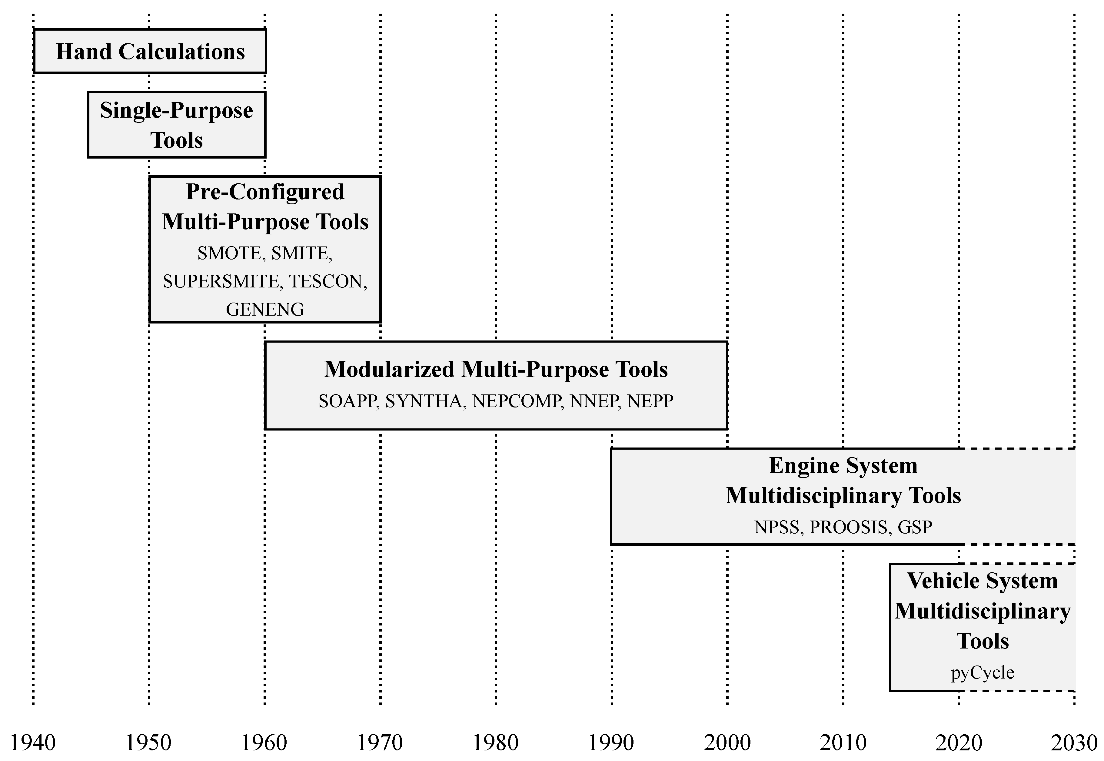
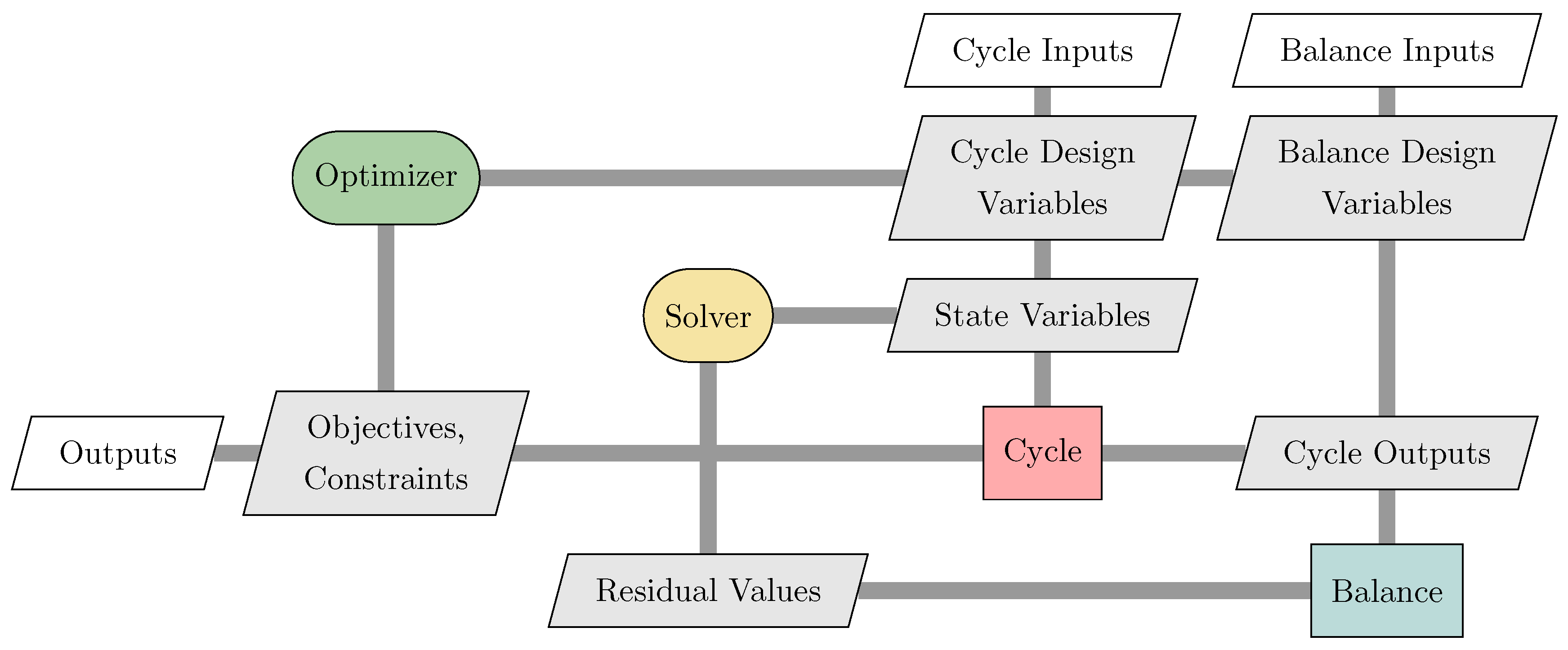
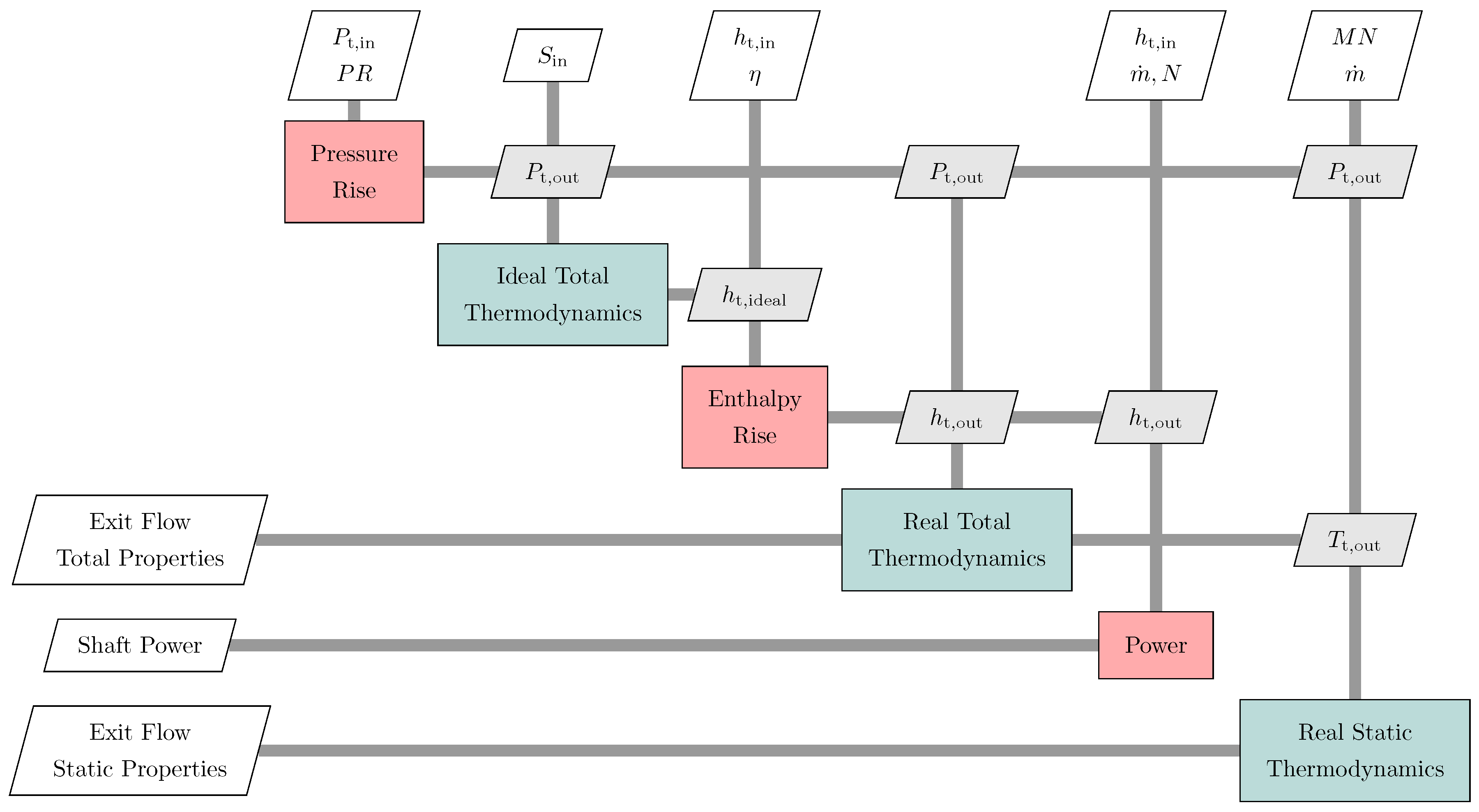
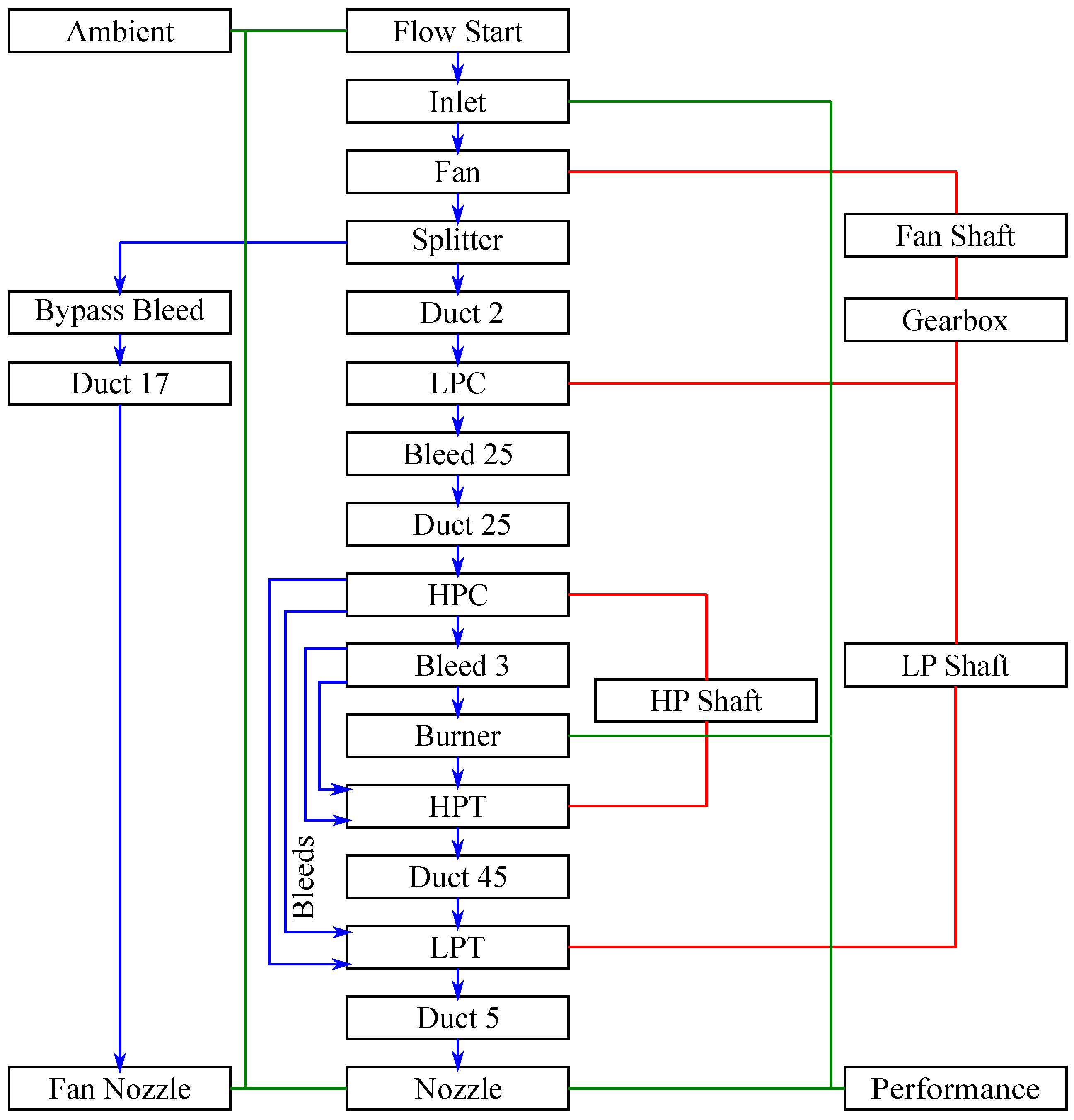
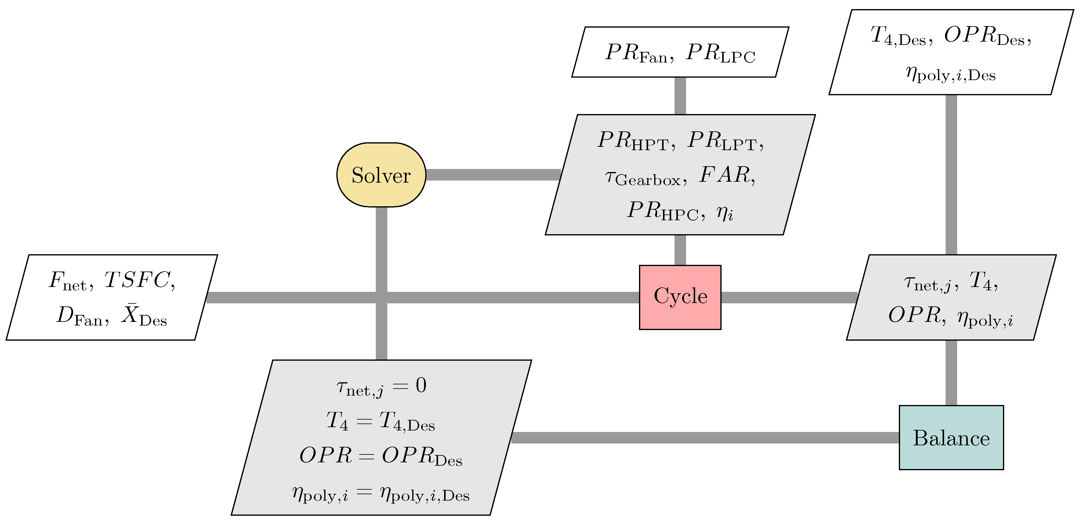
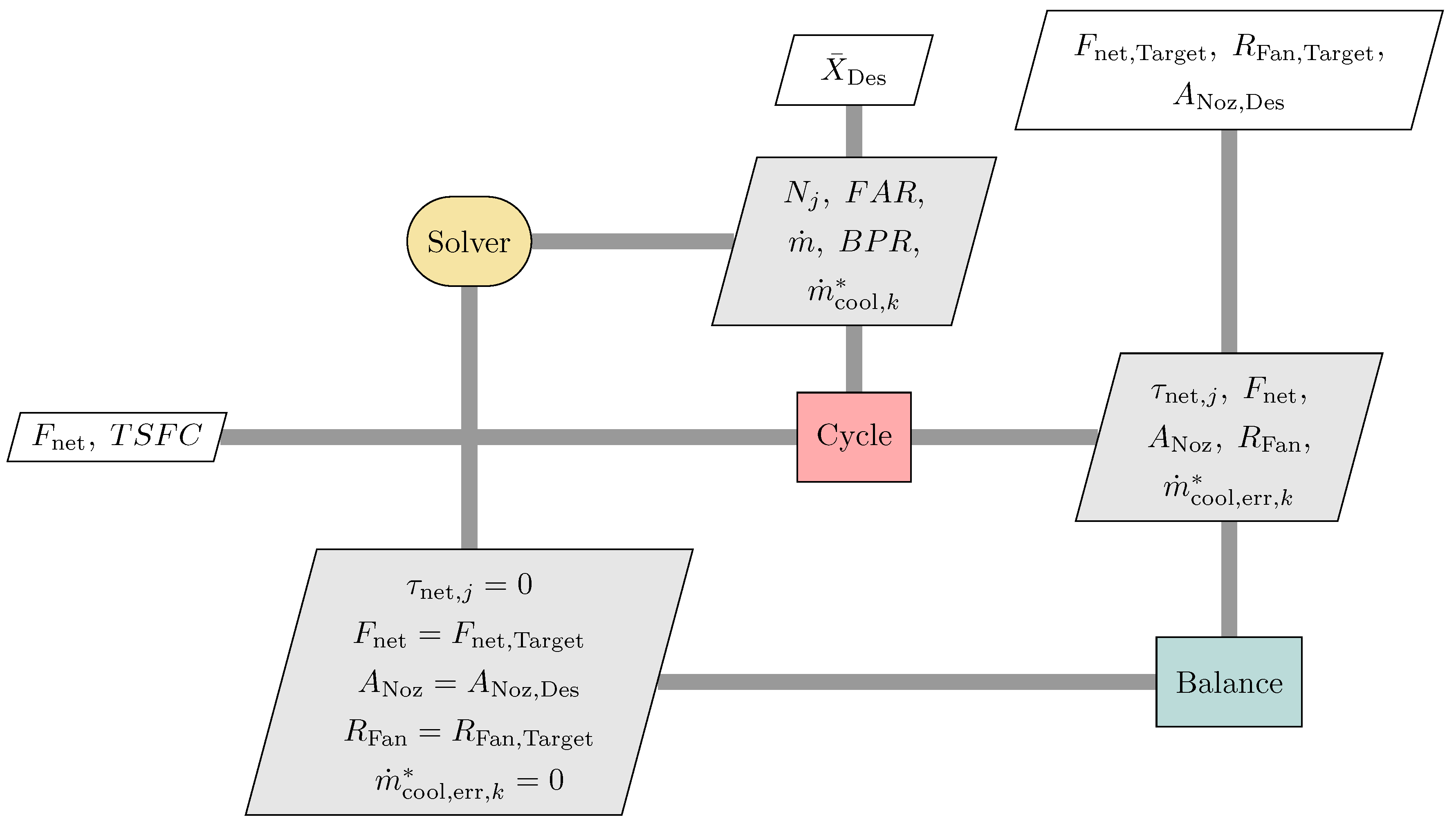
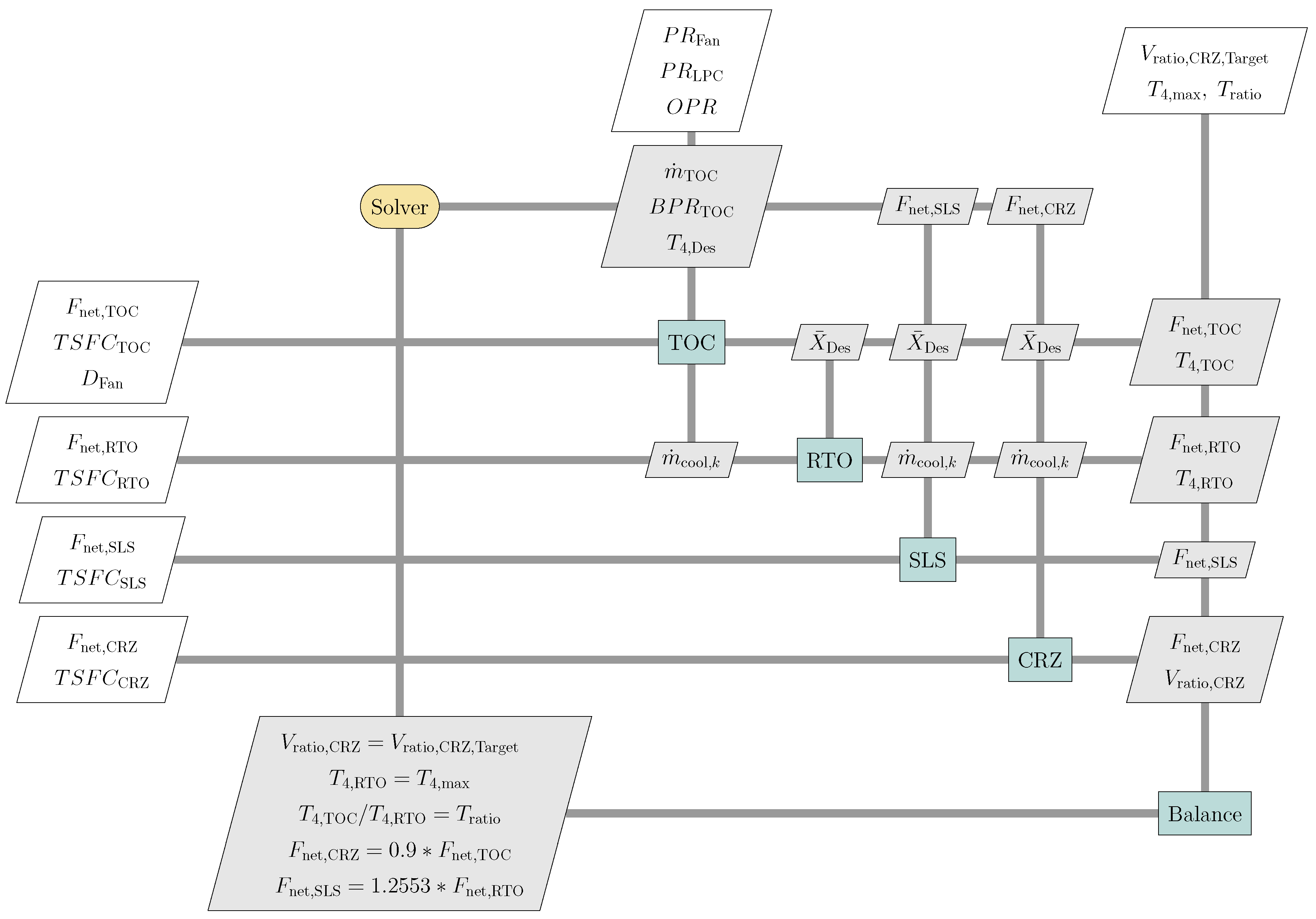
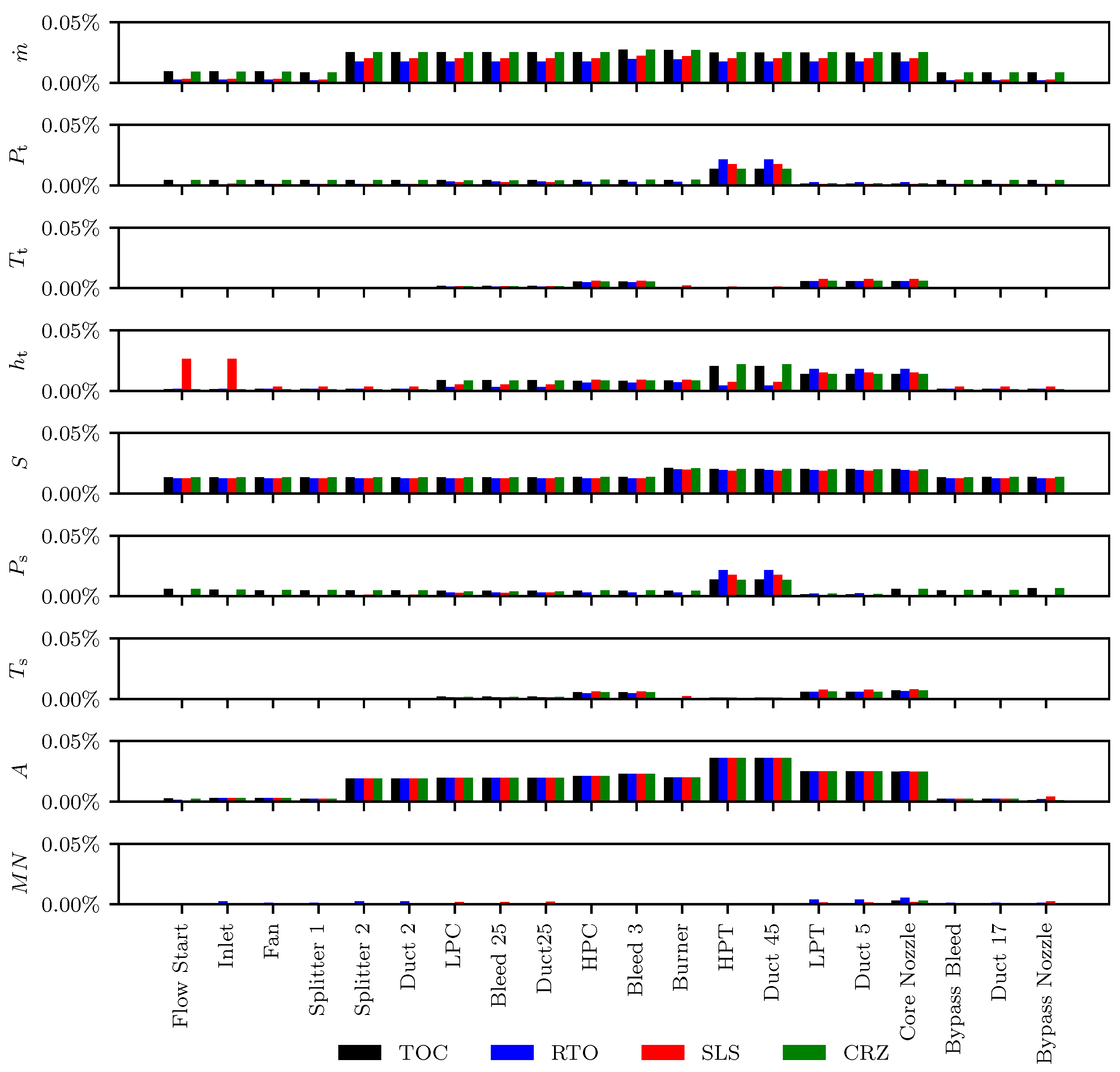
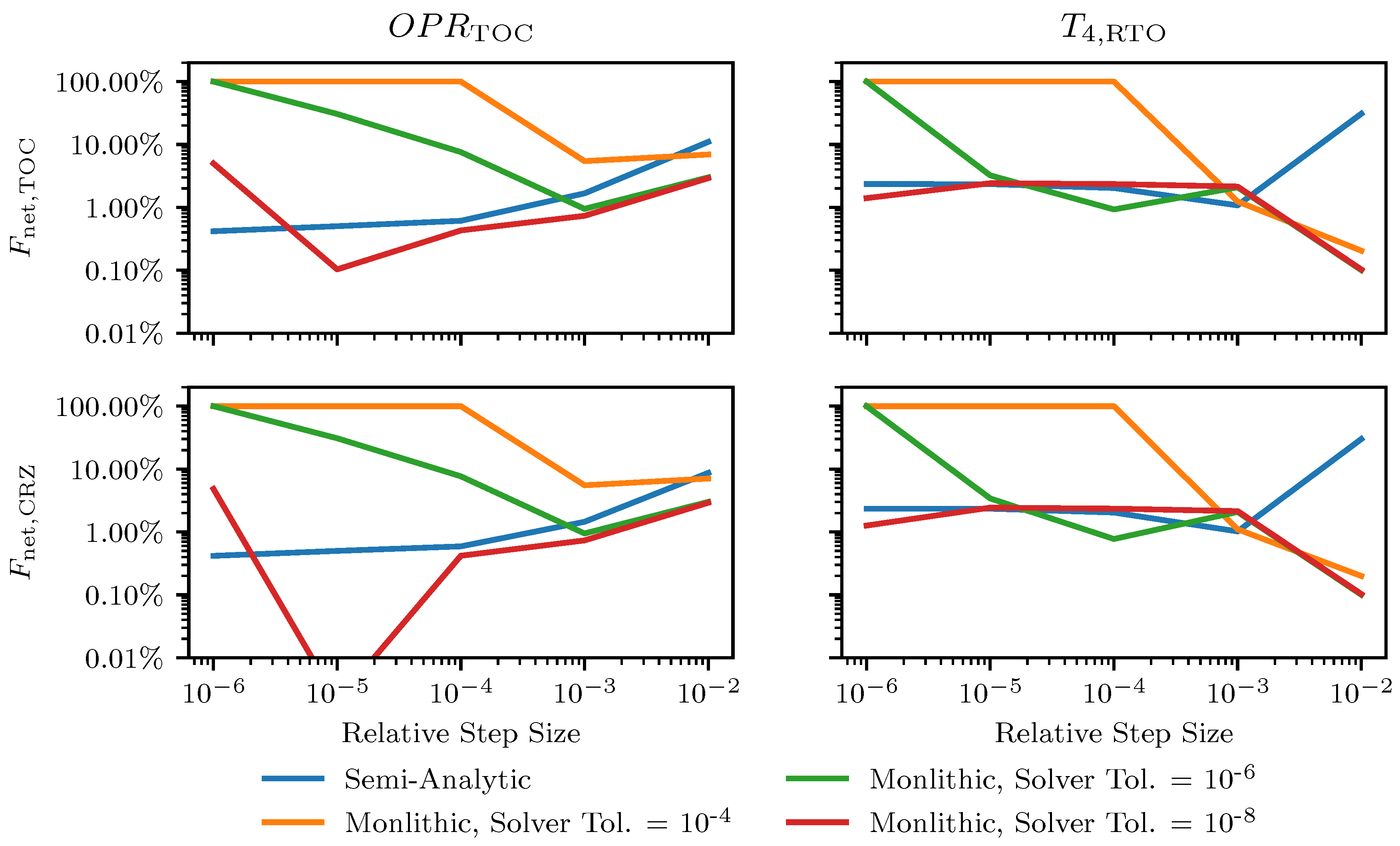
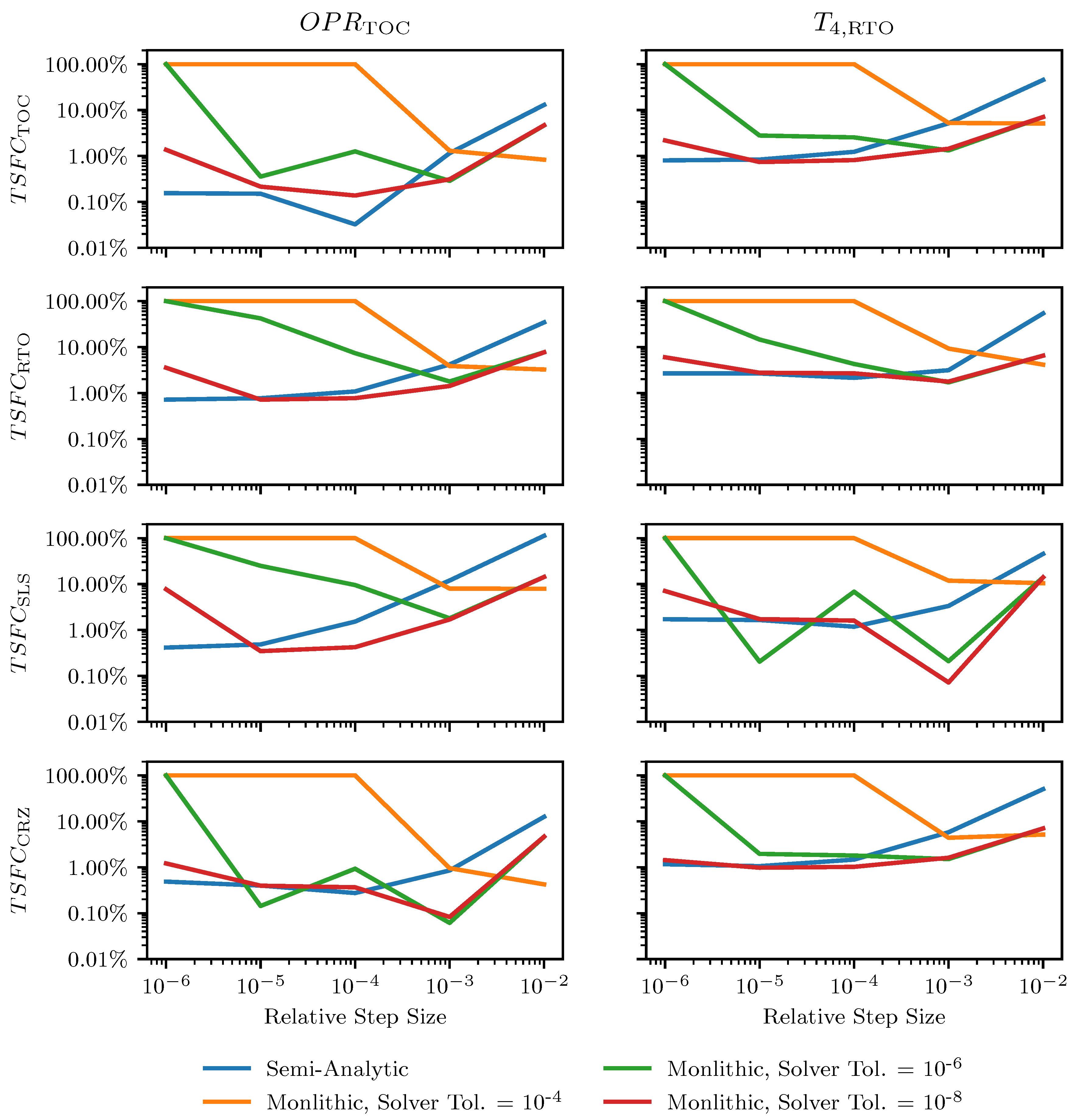
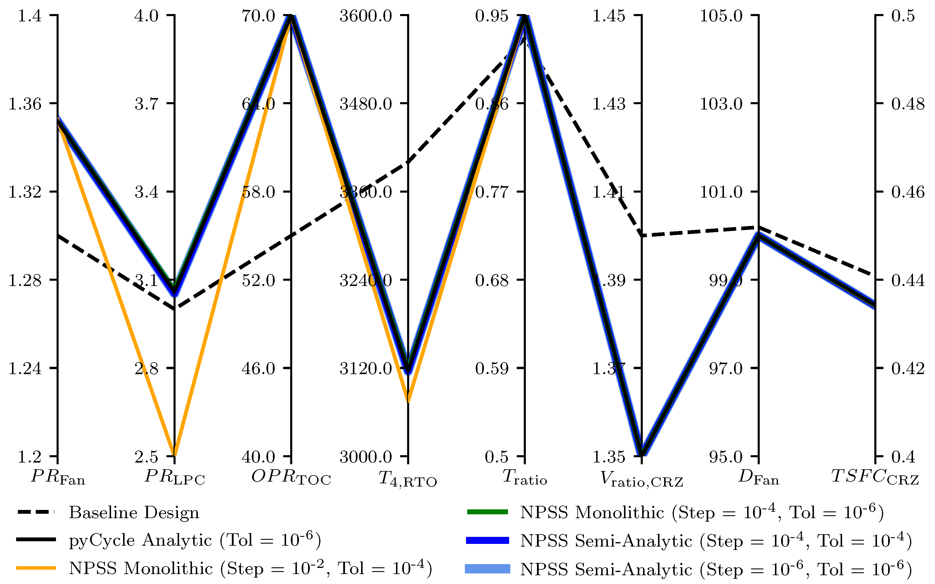
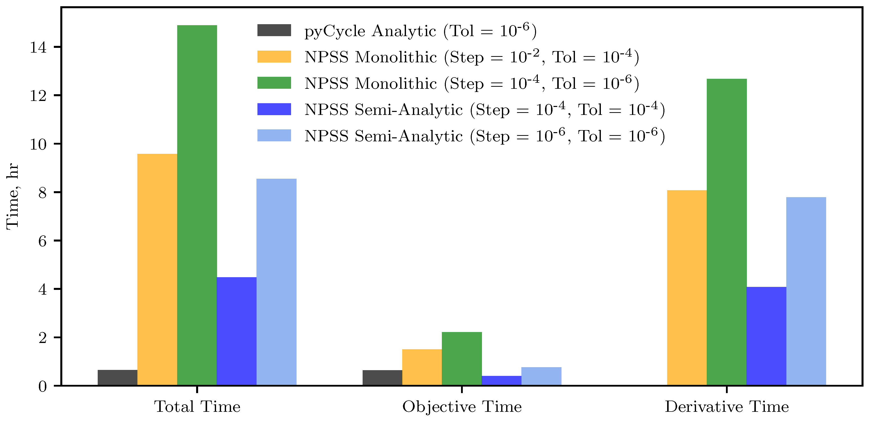
Table 1.
General mathematical problem formulation for the optimization of a turbine engine cycle.
| Variable/Function | Description | |
|---|---|---|
| minimize | f | objective (e.g., Thrust specific fuel consumption (TSFC)) |
| with respect to | x | design variables |
| state variables for physical governing equations | ||
| state variables for conservation laws | ||
| state variables for design rules | ||
| subject to | physical governing equations (e.g., thermodynamic equilibrium) | |
| conservation laws (e.g., conservation of energy) | ||
| design rules (e.g., thrust requirements, stall margin) | ||
| design constraints (e.g., temperature or rotational speed limits) |
Table 2.
Solver problem formulation.
| Variable/Function | Description | |
|---|---|---|
| given | x | design variables |
| find | y | implicit state variables |
| such that | residual equations |
Table 3.
Reduced-space optimization problem formulation.
| Variable/Function | Description | |
|---|---|---|
| minimize | f | objective |
| with respect to | x | design variables |
| subject to | design limits |
Table 4.
Relative difference between pyCycle and NPSS performance properties for the MDP N + 3 reference engine model.
Table 4.
Relative difference between pyCycle and NPSS performance properties for the MDP N + 3 reference engine model.
| Point | Parameter | NPSS | pyCycle | Rel. Diff. |
|---|---|---|---|---|
| TSFC, lbm/hr/lbf | 0.43856 | 0.43860 | 0.00868% | |
| Net Thrust, lbf | 6125.95 | 6126.66 | 0.01171% | |
| TOC | Ram Drag, lbf | 19,865.04 | 19,866.48 | 0.00726% |
| Gross Thrust, lbf | 25,990.99 | 25,993.15 | 0.00831% | |
| Bypass Ratio | 23.74639 | 23.74246 | 0.01656% | |
| TSFC, lbm/hr/lbf | 0.27364 | 0.27368 | 0.01303% | |
| Net Thrust, lbf | 22,800.00 | 22,800.00 | 0.00001% | |
| RTO | Ram Drag, lbf | 17,047.28 | 17,047.53 | 0.00148% |
| Gross Thrust, lbf | 39,847.28 | 39,847.53 | 0.00063% | |
| Bypass Ratio | 25.58064 | 25.57669 | 0.01546% | |
| TSFC, lbm/hr/lbf | 0.16632 | 0.16635 | 0.01910% | |
| Net Thrust, lbf | 28,620.84 | 28,620.84 | 0.00000% | |
| SLS | Ram Drag, lbf | 61.67 | 61.77 | 0.14949% |
| Gross Thrust, lbf | 28,682.52 | 28,682.61 | 0.00032% | |
| Bypass Ratio | 27.34323 | 27.33845 | 0.01745% | |
| TSFC, lbm/hr/lbf | 0.44075 | 0.44079 | 0.00883% | |
| Net Thrust, lbf | 5513.35 | 5514.00 | 0.01171% | |
| CRZ | Ram Drag, lbf | 19,425.68 | 19,427.05 | 0.00703% |
| Gross Thrust, lbf | 24,939.03 | 24,941.05 | 0.00807% | |
| Bypass Ratio | 24.34212 | 24.33803 | 0.01681% |
Table 5.
Total derivative calculation times.
| Method | Time, Seconds |
|---|---|
| pyCycle Analytic | 1.995 |
| NPSS Monolithic (Step = 10−2, Tol = 10−4) | 1863.86 |
| NPSS Monolithic (Step = 10−4, Tol = 10−6) | 1870.90 |
| NPSS Semi-Analytic (Step = 10−4) | 1269.89 |
| NPSS Semi-Analytic (Step = 10−6) | 1225.90 |
Table 6.
Optimization problem statement.
| Variable/Function | Description | |
|---|---|---|
| minimize | CRZ TSFC, lbm/s/lbf | |
| with respect to | TOC fan pressure ratio | |
| TOC LPC pressure ratio | ||
| TOC overall pressure ratio | ||
| RTO combustor exit temperature, R | ||
| Throttle ratio () | ||
| CRZ jet velocity ratio () | ||
| subject to | Fan diameter, in | |
| Top-of-climb thrust, lbf |
Table 7.
Optimization results for the N + 3 reference engine.
| Parameter | Baseline | pyCycle Analytic | NPSS Monolithic | NPSS Semi-Analytic | ||
|---|---|---|---|---|---|---|
| Relative Step Size | - | - | 10−2 | 10−4 | 10−4 | 10−6 |
| Solver Tolerance | - | 10−6 | 10−4 | 10−6 | 10−4 | 10−6 |
| Major Iterations | - | 8 | 12 | 10 | 7 | 7 |
| Total Time, sec | - | 2334.26 | 34,459.95 | 53,609.77 | 16125.09 | 30,767.89 |
| Objective Time, sec | - | 2289.03 | 5397.51 | 7956.92 | 1434.73 | 2730.60 |
| Sensitivity Time, sec | - | 44.79 | 29,061.89 | 45,652.28 | 14,690.11 | 28,036.97 |
| 1.3000 | 1.3519 | 1.3526 | 1.3518 | 1.3519 | 1.3519 | |
| 3.0000 | 3.0590 | 2.5 | 3.0646 | 3.0532 | 3.0534 | |
| 55.0 | 70.0 | 70.0 | 70.0 | 70.0 | 70.0 | |
| , R | 3400.00 | 3115.76 | 3074.84 | 3118.06 | 3115.77 | 3115.55 |
| 0.9265 | 0.9500 | 0.9500 | 0.9500 | 0.9500 | 0.9500 | |
| 1.40 | 1.35 | 1.35 | 1.35 | 1.35 | 1.35 | |
| , in | 100.1907 | 99.9984 | 100.0000 | 100.0000 | 100.0000 | 100.0000 |
| , lbm/hr/lbf | 0.44079 | 0.434154 | 0.434088 | 0.434104 | 0.434104 | 0.434104 |
© 2019 by the authors. Licensee MDPI, Basel, Switzerland. This article is an open access article distributed under the terms and conditions of the Creative Commons Attribution (CC BY) license (http://creativecommons.org/licenses/by/4.0/).
Share and Cite
MDPI and ACS Style
Hendricks, E.S.; Gray, J.S. pyCycle: A Tool for Efficient Optimization of Gas Turbine Engine Cycles. Aerospace 2019, 6, 87. https://doi.org/10.3390/aerospace6080087
AMA Style
Hendricks ES, Gray JS. pyCycle: A Tool for Efficient Optimization of Gas Turbine Engine Cycles. Aerospace. 2019; 6(8):87. https://doi.org/10.3390/aerospace6080087
Chicago/Turabian StyleHendricks, Eric S., and Justin S. Gray. 2019. "pyCycle: A Tool for Efficient Optimization of Gas Turbine Engine Cycles" Aerospace 6, no. 8: 87. https://doi.org/10.3390/aerospace6080087
Note that from the first issue of 2016, this journal uses article numbers instead of page numbers. See further details here.