
Comparing Different Resonant Control Approaches for Torque Ripple Minimisation in Electric Machines

1
Department for Aeronautical and Automotive Engineering, Loughborough University, Loughborough LE11 3TU, UK
2
Wolfson School of Mechanical, Electrical and Manufacturing Engineering, Loughborough University, Loughborough LE11 3TU, UK
3
School of Mechanical and Manufacturing Engineering, University of New South Wales, Sydney, NSW 2052, Australia
*
Author to whom correspondence should be addressed.
Actuators 2022, 11(12), 349; https://doi.org/10.3390/act11120349
Submission received: 31 October 2022
/
Revised: 23 November 2022
/
Accepted: 25 November 2022
/
Published: 27 November 2022
(This article belongs to the Special Issue 10th Anniversary of Actuators)
Abstract
:Electric machines are highly efficient and highly controllable actuators, but they do still suffer from a number of imperfections. One of them is torque ripple, which introduces high frequency harmonics into the motion. One (cost- and performance-neutral) countermeasure is to apply control that counters the torque ripple. This paper compares several single-input single-output (SISO) control approaches for feedback control of torque ripple of a Permanent Magnet Synchronous Machine (PMSM). The baseline is PI (proportional-integral) control, which does not suppress torque ripple, and the most popular control approach is proportional-integral resonant (PIR) control. Both are compared to an advanced PIR controller (PIRA), frequency modulation, a mixed sensitivity design, and an iterative learning controller (ILC). The analysis demonstrates that PIR control, mixed sensitivity state feedback, and the modulating controller achieve identical behaviour. The choice between these three options is therefore dependent on preferences for the design methodology, or on implementation factors. The PIRA and the ILC on the other hand show more sophisticated behaviour that may be advantageous for certain applications, at the expense of higher complexity.
1. Introduction
This paper deals with problem of suppressing torque ripple in electric machines using feedback control. Torque ripple is a serious problem with electric machines, and it can come from a variety of sources, from cogging torque with stator teeth over harmonics in the back-EMF curve to defficiencies in the control scheme [1,2].
Different methods have been proposed to deal with this problem. Constructive measures are able to reduce torque ripple, but they often have a financial cost and a performance impact [3]. Feedforward control is commonly used in industry, where either a back-EMF curve different from a sinusoid is assumed [4], or a current is added based on the rotor position [5]. Any open loop approach will require extensive callibration work to be effective, and it is sensitive to product-to-product variaton [6,7].
For this reason, this paper follows a closed-loop control approach. It starts with a simplified control challenge of suppressing the torque ripple using a closed loop approach by controlling the voltage of the motor based on the speed measurement. In addition to a baseline proportional integral (PI) controller that is not able to address this challenge, four control laws are considered. The first is a conventional proportional-integral resonant controller (PIR), the second is a similar structure using a Mixed Sensitivity Loop Shaping approach. Then, a resonant controller is tested based on a demodulation and remodulation stage. Finally, an Interative Learning Controller (ILC) with a delay block is considered.
This covers the most common feedback controllers for torque ripple, but is limited by choice to linear approaches. Self-optimising controllers are excluded from consideration, because they always contain a non-linear element for the adaptation, and thus show more complex behaviour.
This work is novel in that for the first time it compares these different approaches to torque ripple minimisation starting from first principles. It is the first paper to prove that the resonant controller is exactly identical to a modulating controller. Furthermore, the detailed analytical and simulated comparison of controller simulations has not been seen before in the literature.
2. Materials and Methods
The aim of this paper is to compare different control approaches for reducing torque ripple in an electric machine algebraically, and then to compare their performance using simluations.
To keep the problem simple, a very basic model of the permanent magnet synchronous machine (PMSM) is used, which abstracts from the phase voltages and the inner control, instead focusing on the speed control loop. [8] A list of the symbols used can be found in Appendix A.
The plant is defined as a first order low pass filter capturing the key mechanical dynamics of the rotor:
The input is the driving voltage for the motor (), and the output is the shaft speed. In the interest of simplicity, time delays and the electrical time constant are ignored, but they could be added easily (and they may be relevant for the loop response at resonant frequency). The time constant of the first order low pass (PT1) is the result of the damping effect of the winding resistance acting on the inertia of the rotor. This model ignores the electrical time constant caused by the motor inductance in the interest of simplicity, but the same approach can be applied to more complex plant models.
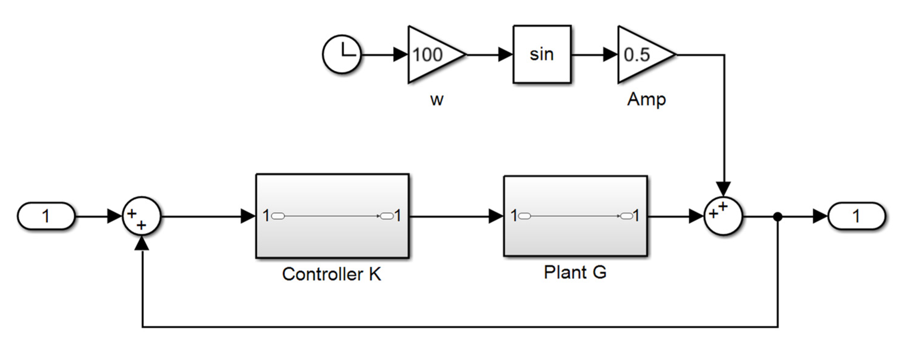
The torque ripple is modelled as an external disturbance at a known frequency, acting onto the plant. This enables to stay within a linear framework, while a speed/position dependent model of the ripple would require a non-linear analysis. For constant speed operation or for moderately slow speed changes, this approach is perfectly sufficient. It leads to a structure as shown in Figure 1.
The disturbance could also be generated by a resonator without damping, with equal results. It is worth noting that this resonance is not connected to the control input, which means it does not become part of the feedback loop. This makes resonant control fundamentally different from the control of resonant plants, as discussed in [9].
This simple structure allows to compare different controllers for their ability to deal with the ripple torque, without making too many assumptions about the specific motor behaviour.
3. Methodology
3.1. Baseline Control
Single-input single-output (SISO) control design typically starts with a PI controller for a low pass plant, and we will follow this approach here.
Additionally, the corresponding PI controller is
Conventional tuning would be based on cancellation of the dominant pole, which means that and therefore the open loop chain is
The bandwidth is set via , and a typical choice would be , leading to a closed-loop time constant of 0.1 s (and a control bandwidth of rad/s). This would not be enough to make any difference to the ripple frequency.
It is possible to push the control bandwidth higher to achieve decent attenuation of the ripple frequency, but this would require a very high control gain. This may reduce the robustness of the controller, and it may introduce significant sensor noise into the control loop and therefore the system output. More targeted approaches to suppress the ripple will be presented below.
3.2. Resonant Control
The conventional approach to eliminating torque ripple is resonant control [10,11], which is based on a resonant second-order filter of the form
As long as there is clear separation between the operating frequencies of the PI branch and the resonant branch, both options produce very similar results for a single resonant frequency, with only some higher order differences that are typically negligible. However, if several ripple frequencies have to be eleminated, the parallel form has a distinct advantage, because they are treated independently. Although the problem considered here concerns only one frequency, the parallel form is used here for its easy of extension to several frequencies.
Note that the phase at resonance is adjusted via the proportion of a and b, and unfortunately this has an impact on the amplitude response. This connection between phase and amplitude is the main complication when designing a PIR controller.
The operating principle of this filter is to bring up the loop gain above one at the resonance frequency to reduce the loop sensitivity function at this frequency. The structure satisfies the internal model principle, which states that an effective controller has to include a model of the disturbance it is targeting, which the resonator in the PIR controller achieves. Unlike a normal controller, which has a limited bandwidth denoted by the unity open loop gain , a resonant controller intersects this limit several times, leading to several discontinuous frequency ranges of operation. In other words, the resonant controller operates at low frequencies and at the resonant frequency, but not in the frequency range in between, where it has a very low gain.
The design of the resonant filters differs slightly between the parallel and series configuration. The parallel design usually follows two independent design processes for the two branches, where the other branch is treated as a small disturbance. This requires clear separation between the control bandwidth of both controllers, specifically .
If the separation is not as clear, a serial design process is indicated, where one controller is designed first, and the second controller is designed for an extended plant including the first controller. This approach works for the series connection of the resonant controller, which can be interpreted as a second order phase lag filter.
One of the challenges of designing a resonant controller is to get the phase of the control action right. In theory, this can be tuned via the nominator coefficients and , but these also have an impact on the magnitude response.
Alternatively, an all-pass filter or a phase lead compensator can be added to delay the phase without affecting amplitude, while keeping . This leads to the following form, which has more consistent amplitude behaviour at the expense of another state:
This controller will be called PIRA (PIR with phase Advance). It presents significantly different behaviour from the basic PIR controller.
3.3. Mixed Sensitivity Design
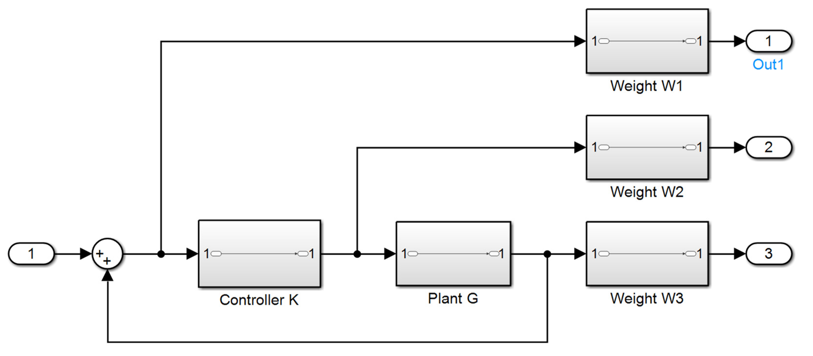
Mixed Sensitivity Loop Shaping is an optimal controller design approach coming out of robust multiple input multiple output (MIMO) control. It is based on an extended plant model that contains both the plant model and weights to tune the optimisation problem for specific areas. Three weights are used: shapes the sensitivity function, reduces the control energy, and shapes the co-sensitivity function. The full structure is shown in Figure 3.
It is standard to use an integral weight in to force reference tracking, possibly in connection with a constant weight.
and to start with a constant weight on the input
For the suppression of torque ripple, an additional weight based on is added to to respond to this ripple frequency:
Together with the original plant, this leads to the following state space model for the extended plant (the bold symbols denote matrices and vectors):
with
The first state is the state of the original plant. The second state is the integral weight , and the last two states belong to .
Typical loop shaping designs are robust and therefore based on the norm. However, for simplicity reasons, we will use the norm here, because it leads to a convex optimisation problem and a low order controller. A state feedback controller is designed following a standard LQR approach, with a control law of the structure
Since the weights are not physical, they have to be copied into the controller to complete the transfer function. In this example, all states are known (measured or simulated), and therefore no state observer is required. The resulting transfer function of the controller is
which shows exactly the same structure as the PIR controller. This means it will produce the same potential performance, just via a different design approach. The inclusion of the resonator from the weight in the extended plant into the controller again satisfies the internal model principle.
The advantages of the mixed sensitivity design are shared with most optimal control approaches: the user only has to specify the control objectives, and the optimal design process will synthesis a controller to achieve these. Stability is guaranteed, as is robustness (within limits).
3.4. Modulating Controller
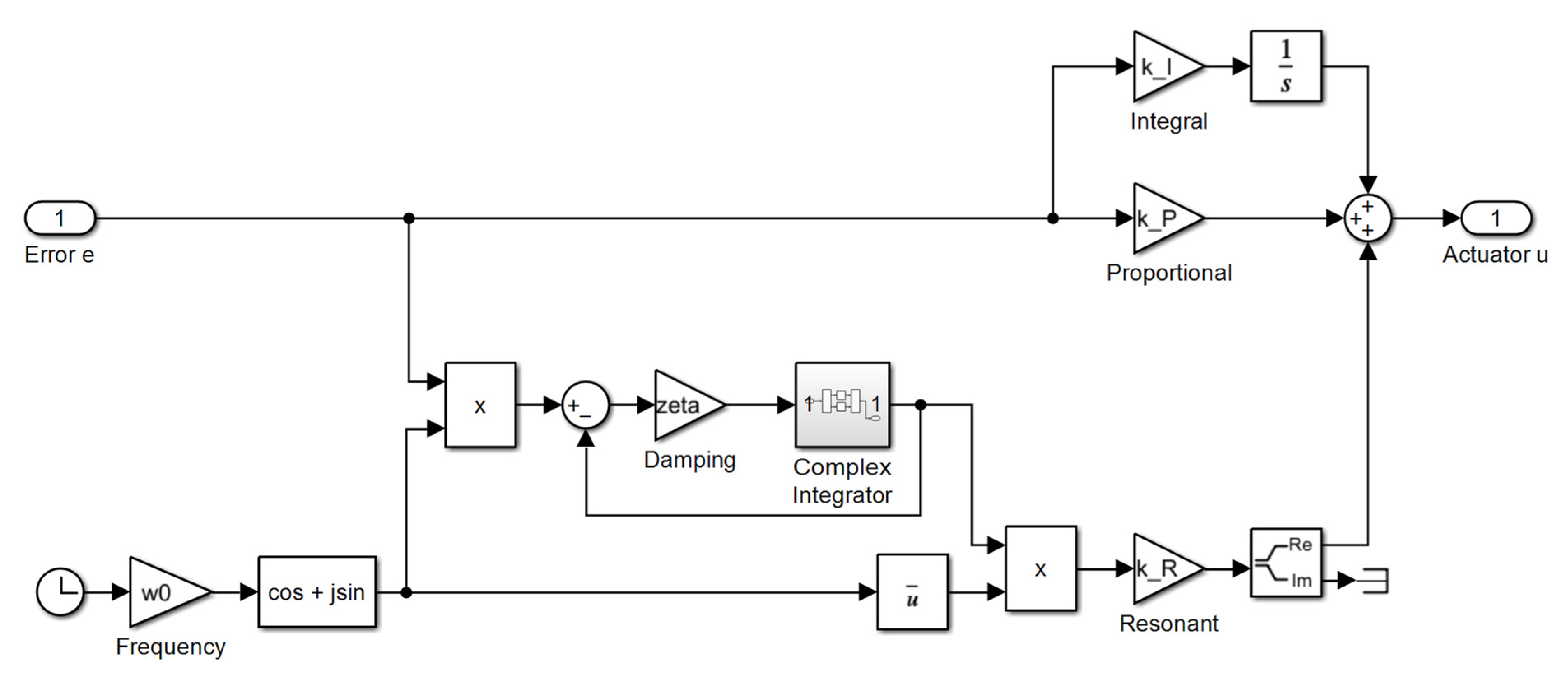
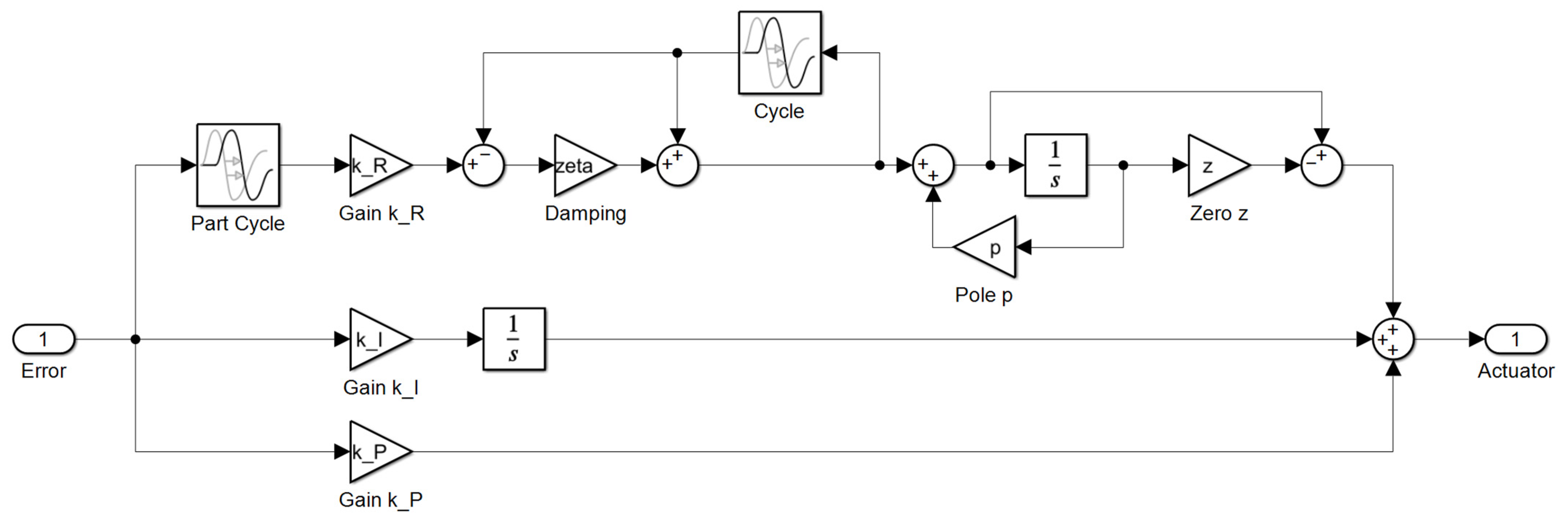
A different approach found in the literature is to use modulation with a carrier frequency to inject a precisely designed signal to cancel out the torque. This approach originates from open-loop approaches of torque ripple compensation [12], and it adds an integral controller to make the cancellation signal adaptive [13]. A typical block diagram is shown in Figure 4.
Note that the integrator operates on a complex signal, and the standard integrator in Simulink does not support this, so it has to be replaced with a custom-made integrator block. It is possible to separate the sine and cosine and run them through separate integrators, but the complex signals make for a much easier analysis.
The transfer function of a modulating controller can be calculated using careful algebraic manipulation. We start with an input signal of
where is the input phasor, and its conjugate. The modulation with the carrier
leads to
Note that this is a complex signal. For practical purposes, it may be split into a real and imaginary component, but this is not necessary for the analysis. A first order low pass filter is applied with the transfer function
This has to be done separately for the two frequencies, leading to
This signal is modulated back into the desired frequency by dividing by the carrier (or multiplying with its conjugate):
This signal has imaginary components, and we are not interested in that. Instead, we only use the real part:
This establishes the transfer function of the modulating controller to be
Again, this transfer function is identical to the structure of the PIR controller, which means that the same control performance can be achieved. By matching the specific parameters, it can be matched exactly to the transfer of the resonant controller by adjusting and accordingly. Note that the phase can be adjusted using , and this has exactly the same effect as and in the PIR.
What may be remarkable is that there are no modulation artefacts, no harmonics, no cross-modulation: the output is again a pure sinusoid. This is because the second modulation is a division, and not a multiplication, and therefore the harmonics of the carrier do not appear in the output.
Despite being identical to the PIR in behaviour, there are three distinct advantages to this implementation of the modulating controller. The first one is that the actual controller works on a low bandwidth signal, so it could have lower sampling rate. The second is that the frequency is easy to adjust. For a variable speed motor, the modulating controller only needs the rotor position, which is always known for a synchronous machine. Finally, the compensation of phase lag in the plant is easy by just tuning the complex gain . This phasor can be frequency dependent, based on a simplified model of the transfer function of the plant.
3.5. Iterative Learning Control
Iterative Learning Control (ILC) is a control approach developed for cyclical reference signals, exploiting the fact that the cycles are always the same. By knowing the response to the previous cycle, the response to the next cycle can be planned without the causality constraints usually in effect. This approach can also be used to deal with cyclical disturbances, as long as the frequency is known [14,15].
The key element of an Iterative Learning Controller is a delay block that delays the signal by the duration of one period . This allows the controller to respond to deviations during the previous cycle. It is often used in an iterative way such as
which adds the new input signal to the output from the previous cycle, which creates a basic linear adaptation or learning capability.
A key advantage is that can be adjusted either up or down to account for phase differences when going through the plant. An important feature of ILC is that it shows the typical “comb” pattern of the delay block in the amplitude plot of a closed loop, which means that it works for a fundamental frequency and all its harmonics. This can be an advantage, especially for electric machines that can show a range of harmonics (and DC or low frequency signals). At the same time, it can also be a concern, because the response at these frequencies cannot be tuned separately, and this can lead to unwanted interaction with high frequency plant dynamics.
Just as with the resonant filter, adjusting the phase of the ILC is not easy. It may be tempting to add a time delay to control the phase, but this tends to lead to large phase lags that affect the stability of the loop, especially given that the ILC has a significant steady state gain. A typical control structure would be as shown in Figure 5, and the resulting control law is
Note that this control law has essentially the same parameters as the advanced resonant controller, but the parametrisation may have to be different. This is because the resonant controller operates at all multiples of the resonant frequency, including the frequency 0. Thus it replaces the proportional action of the PI controller, but not the integral branch. This is mostly a consequence of this controller being significantly more powerful than the previous examples.
Especially with complex plant models, further filtering and compensation will be required to guarantee stability at all resonant frequencies. In this sense, the ILC controller is very similar to a high bandwidth PI controller, but it has the advantage of acting only at the relevant frequencies, keeping the magnification of sensor noise to a minimum.
4. Numerical Results
Unfortunately, an experimental rig was not available to the authors for real-world validation of the above analysis. However, work is progressing in this direction. Therefore, Simulink simulations are presented to give an initial and fair comparison between the different controllers, highlighting key features and demonstrating the correctness of the derivations above. The application of these controllers to an experimental rig is planned for a future paper. All files used to produce these results are available at https://github.com/LU-Centre-for-Autonomous-Systems/resonant_control/, version 1.0, published 27 November 2022.
4.1. Plant
All controllers are applied to the same plant, which is a simplified model of an electric motor, with the structure given in (1). The transfer function is a PT1 low pass filter with a time constant of 1 s, a gain of 1, and a ripple frequency of 100 rad/s.
A sinusoidal disturbance with a frequency of 100 rad/s and an amplitude of 1 is added to the output, this represents the effect of the ripple torque:
More complex plant models can be used, and they will impact on the design of the PI controller, but the impact on the resonant controller is mostly limited to the plant behaviour at the resonant frequency.
4.2. Controller Design
To keep the different control structures comparable, the same parameters are used, based on a mixed sensitivity design. The weights are defined as
These weights already contain some important information about the controller. They reflect the ripple frequency of rad/s, and they have a defined damping of , which means that response to the ripple frequency is expected to be very focused, and it will take many periods for the controller to settle. The numerical gains 10 and 50 determine the importance of reference following and resonance suppression. Note that these gains are a lot more sensitive than and in the LQ design, so it would not be appropriate to move in steps of factors of ten. Instead, changes by a factor of 2 were used to determine appropriate gains with an appropriate balance between integral and resonant action.
The mixed sensitivity H2 design leads to a state feedback controller law with
and a transfer function for the resulting controller of
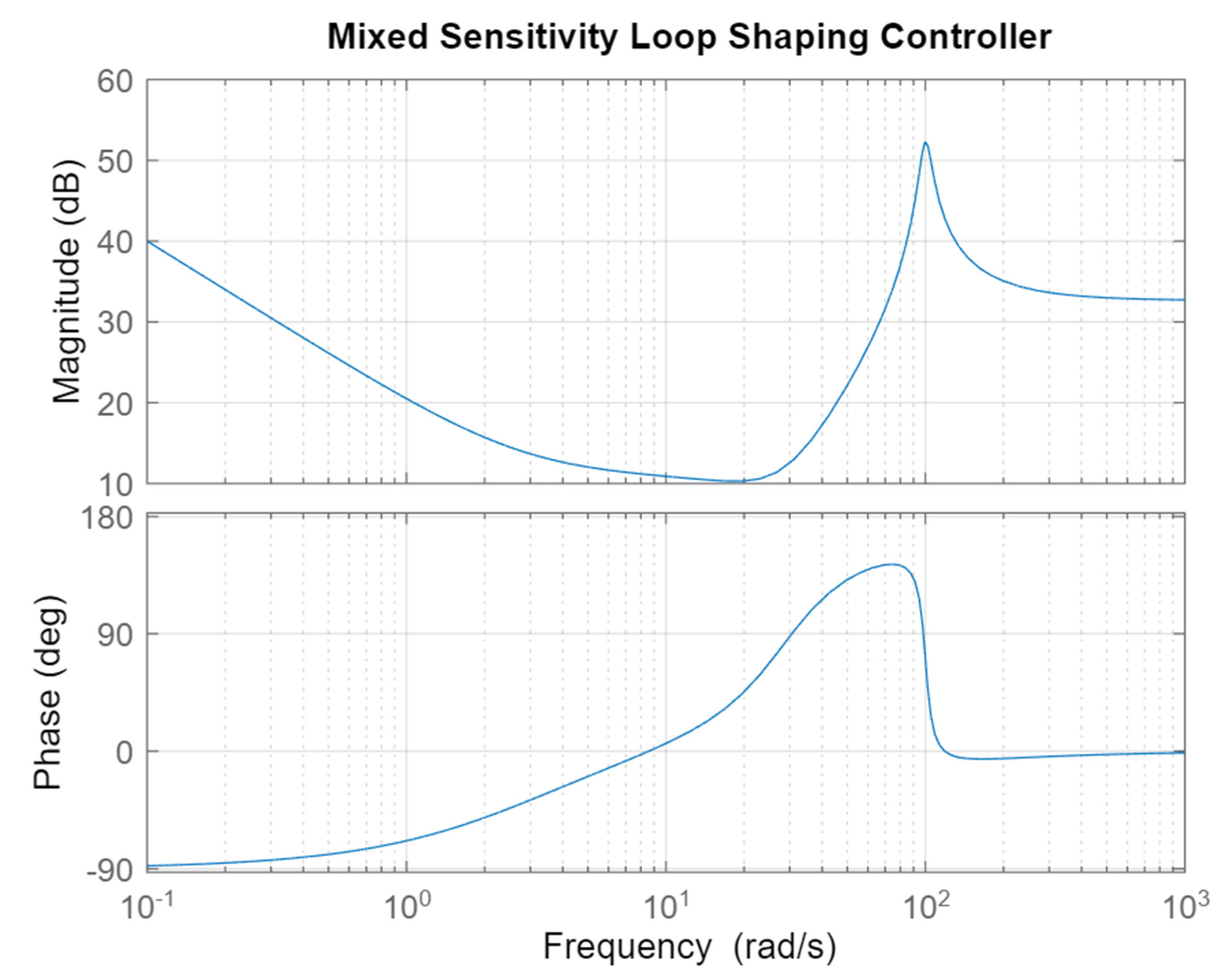
The Bode Plot of this transfer function is shown in Figure 6. From this transfer function, all the controller parameters can be determined:
and all five controller laws can then be calculated to be as similar in effect as possible:
The compensator parameters and the gains for , and are chosen such that the behaviour at the resonant frequency is identical, matching amplitude and phase. The ILC required a slightly different compensator to achieve stability, because the ILC branch has significant steady state gain. Note that the ILC does not have a proportional branch, because it already has proprotional action at low frequencies.
4.3. Open Loop Behaviour
Note that Simulink is unable to derive correct transfer functions for the modulating controller or the ILC, so all diagrams have been numerically derived using a FFT of an impulse response. Through careful choice of the excitation signal, the result should be accurate and free from noise. The phase is not unrolled, so discontinuities are to be expected.
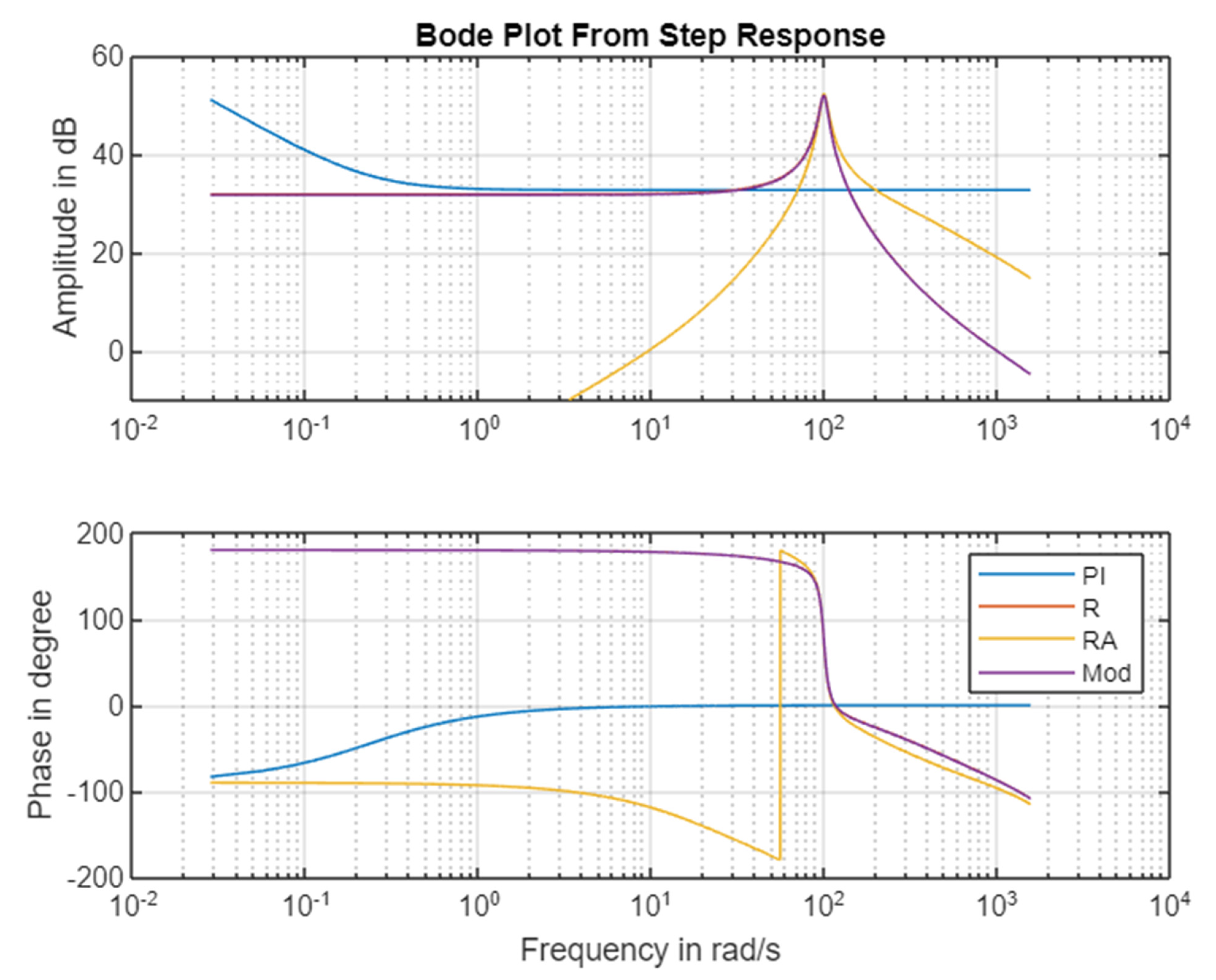
The first observation is that despite different design approaches and different control structures, the PIR controller, the Mixed Sensitivity controller, and the modulating controller have exactly the same transfer function, and therefore the same effect. This is not surprising, given that they have the same structure of the control law, as demonstrated in the previous section, and the parameters were chosen specifically to match the behaviour. Obviously, it would be unsusual to find exactly the same parameters using different design methods, but this paper is about comparison of the potential of different control structures, not design methodologies, so in this case, the matched parameters are appropriate. The resulting behaviour is identical, and this is confirmed on the open loop Bode plot of the different resonant branches of the controllers in Figure 7. The PI branch is drawn out and plotted separately to focus on the behaviour of the resonant branch. Only one line is shown for both the resonant controller and the mixed sensitivity design, because the implementation is in fact idential, while the modulation controller has a completely different implementation, but with the same behaviour.
This plot also shows how different the PIRA controller is with a phase advance compensator. It shows a much stronger roll-off below the resonant frequency, which means that it interfers much less with the low frequency behaviour of the PI branch—but it does have slighty higher gains at higher frequencies, which could potentially affect the robustness.
Because the PIR, MS and modulating controller are indentical, only the PIR controller is considered further, and compared with the PIRA and ILC design. In terms of the design approach, the Mixed Sensitivity design has the advantage that it deals with phase and stability automatically, while these have to be considered as additional complications during the turning of the PIR controller.
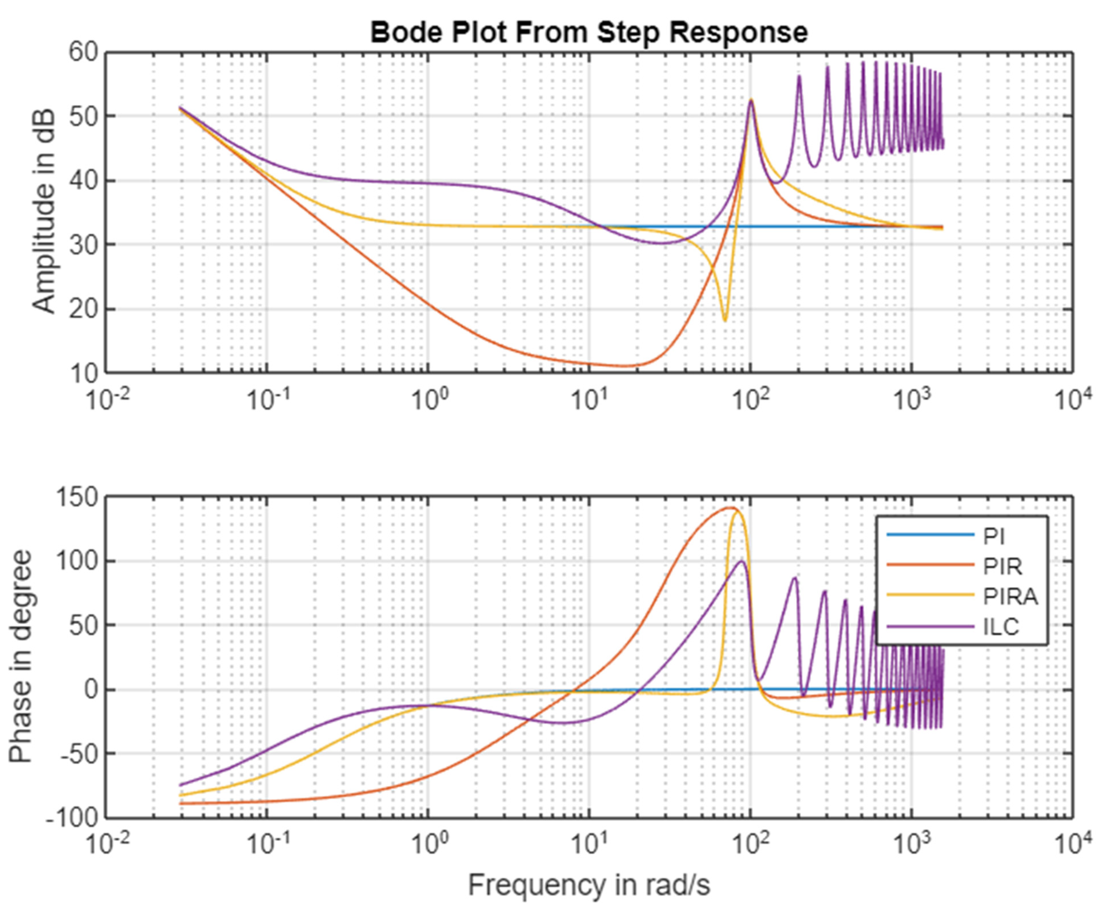
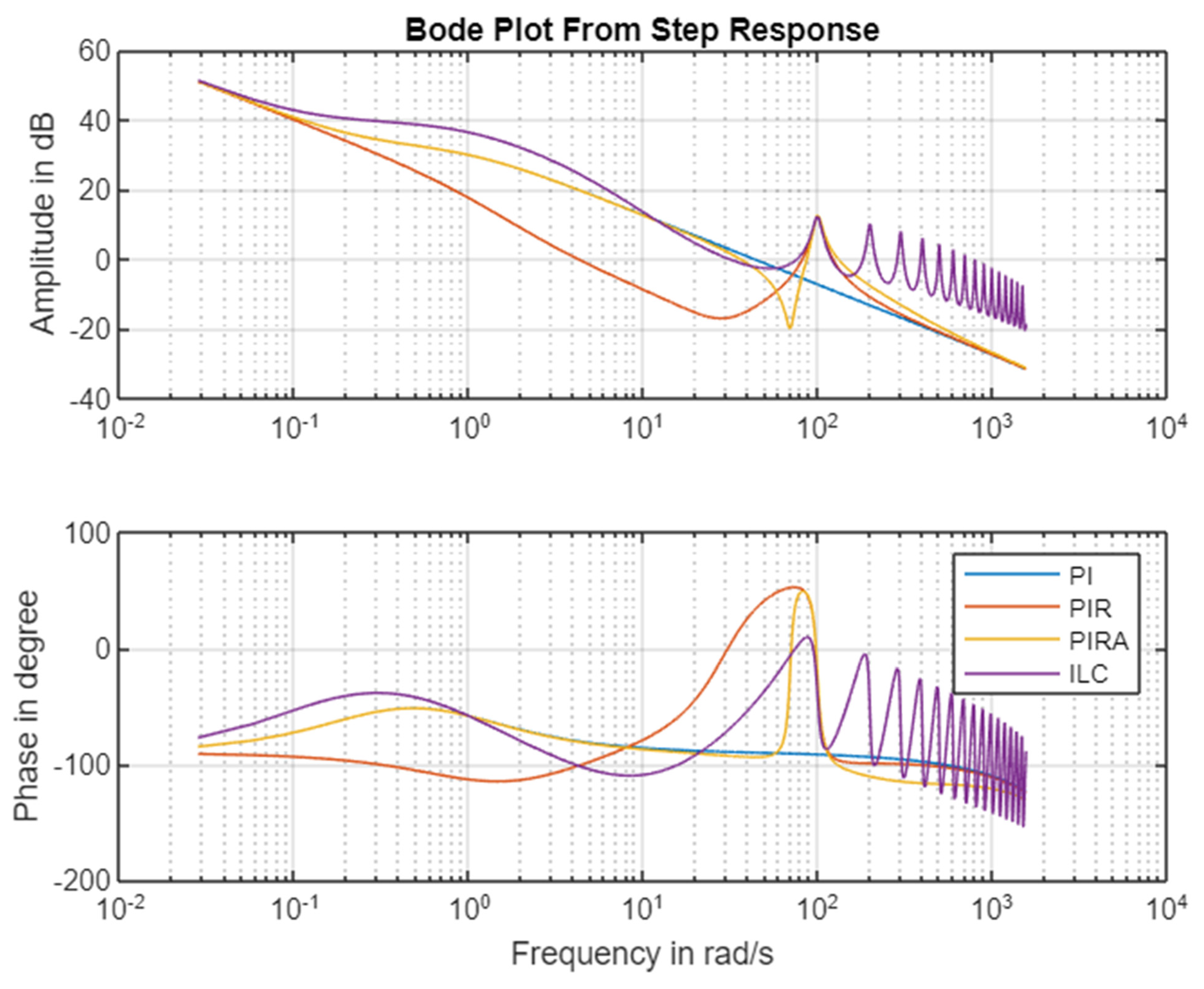
Finally, Figure 8 and Figure 9 shows a comparison of the four different controllers (PI, PIR, PIRA and ILC) for the controller only and for the open loop chain. By including the plant model, this Bode Plot of the open loop chain allows an analysis of the stability and robustness of the different controllers.
The plots highlights both key similarities and differences between the approaches. The PI controller obviously does not address the ripple frequency, this is expected. All other controllers show how the loop gain goes above one (0 dB) again around the ripple frequency, and how the phase is well controlled in this second critical region. The PIR controller achieves the objective, but there is a very significant impact on the operation of the PI controller for low speed operation, which means that the PI controller may have to be retuned after adding the resonant branch. The PIRA avoids this, and preserves the correct operation of the PI branch while also achieving good suppression of the ripple frequency. The ILC finally is very similar to the PIR controller around the resonant frequency, but it deviates from all other controllers both at low frequencies and at harmonics of the ripple frequency, as expected from the theoretical analysis.
The main conclusion is that apart from the PIRA approach, all controllers have interferences between the PI controller and the resonant part, despite the significant frequency separation. The PIRA is the only resonant controller that avoids this interference.
4.4. Closed Loop Behaviour
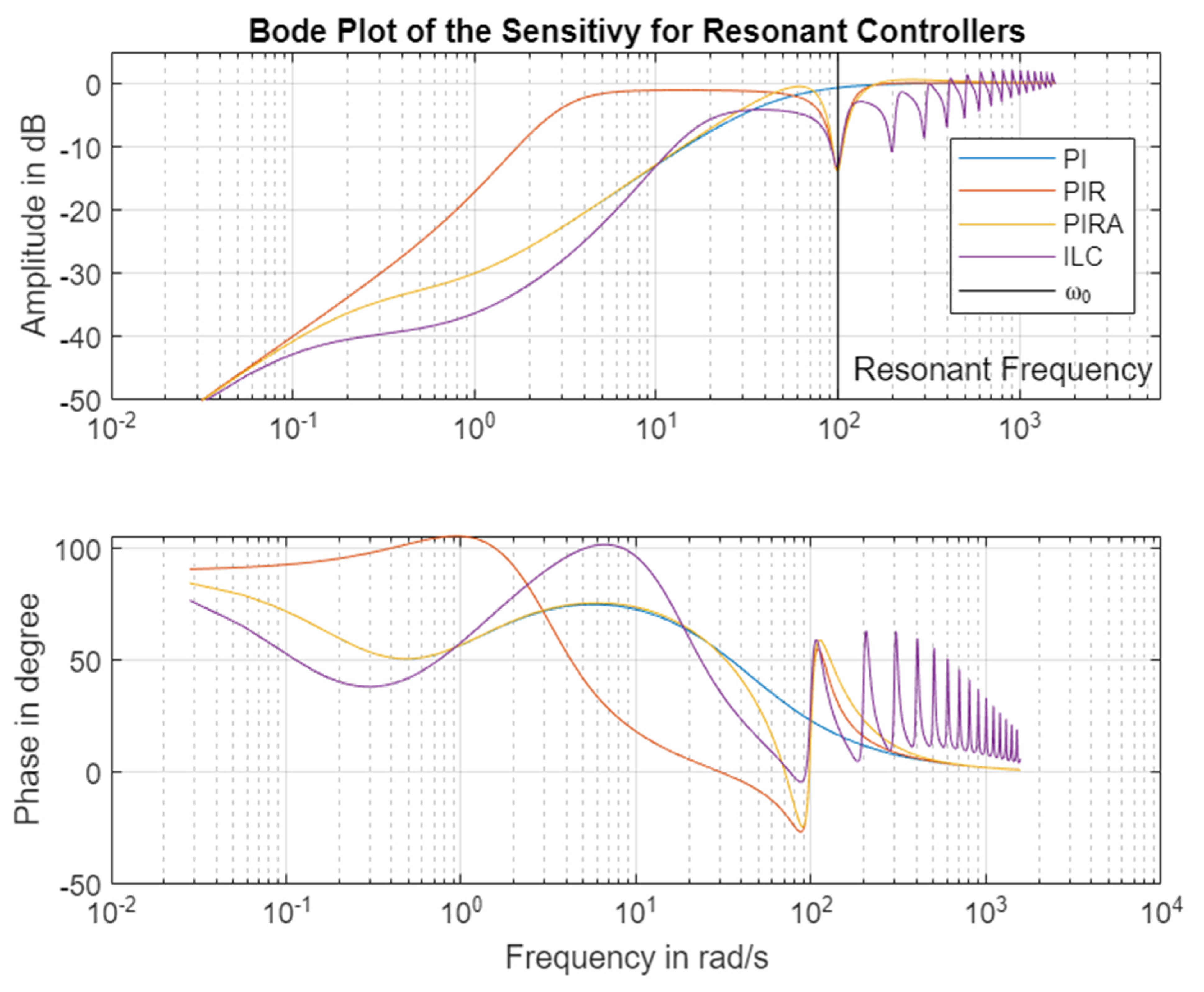
The closed loop behaviour is studied both in the frequency domain and in the time domain. The frequency domain is shown in the Bode plots of the complementary sensitivity function in Figure 10. This shows the transfer of disturbances of the reference on the error signal. The goal is to have a gain as low as possible for low frequencies (reference tracking), and at the ripple frequency, as this would be an indication of successful control. This view again demonstrates how similar the different controllers act around the ripple frequency, and how the resulting loop behaviour is very similar.
All controllers achieve this objective, with the expected exception of the PI controller, which does not address the ripple frequency. The plot also highlights how much influence the resonant controller (PIR) has at low frequencies—so the notion that it can be designed separately from the PI controller is not applicable here. The ILC performs reasonably well, but it is clearly quite different at low frequencies from the other controllers.
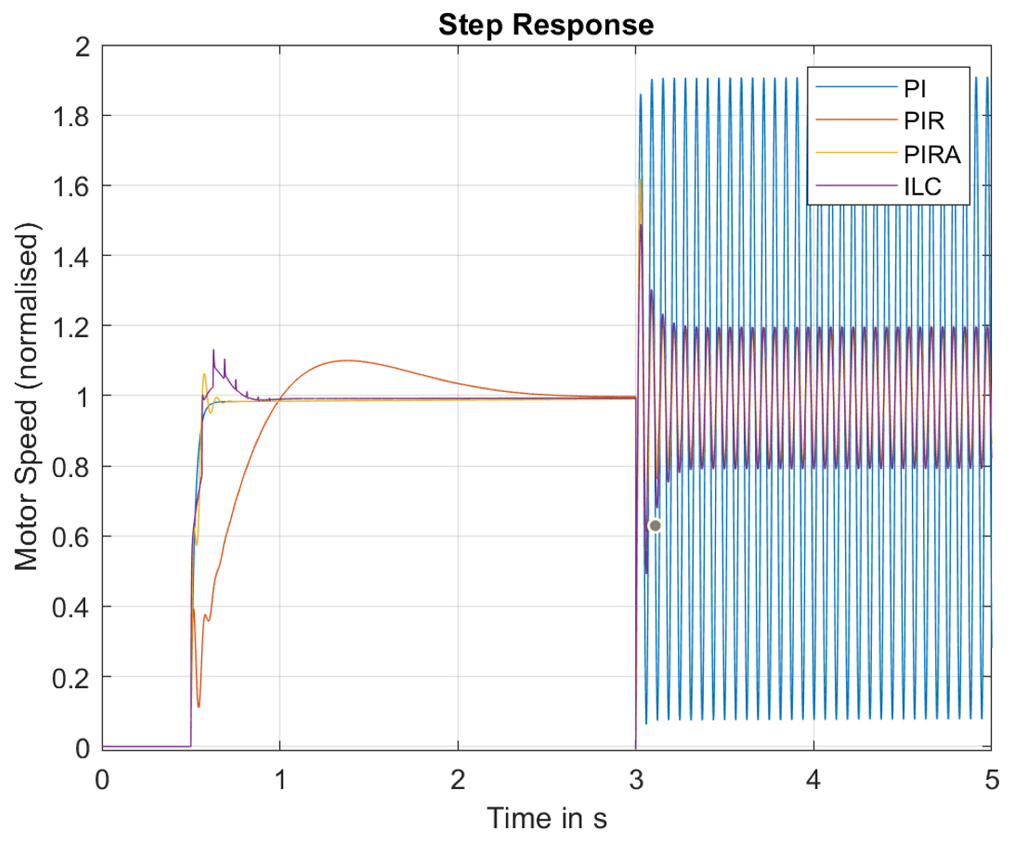
The time domain response is shown in Figure 11. This simulation is subject both to a reference jump at 0.5 s and to a sudden sinusoidal disturbance at 3 s, so it shows a combination of how the system deals with both. This diagrams shows very clearly that the resonant controllers affect the step response. The high frequency content in the step excites the resonance—leading both to some eratic movements and possibly some overshoot not present in the original pure PI controller. Both the PIRA and ILC at least maintain most of the low frequency step response, but it is still not as clean as the PI controller, and they all have some overshoot.
To avoid this, it may be appropriate to apply a low pass filter to the reference input that limits high frequency content. Since that is a feed-forward filter, it does not affect stability, and it can be tuned seperately from the loop.
All controllers except the PI controller achieve good ripple suppression. The time domain view shows very nicely that the ripple suppression needs some time to settle and take effects. This is because the ripple suppression only applies to a very narrow frequency range, and the sudden onset of the ripple disturbance contains a much wider frequency range initially. Stationary behaviour is achieved after about 0.3 s, which means it is a bit slower than the settling time of the PI controller. Usually, fast settling is not required, and this would be considered more than acceptable.
5. Discussion
The paper has compared three very different controllers for the control of torque ripple in an electric machine using a simplified plant model, as well as a baseline controller without this capability.
The most common controller is the resonant controller (PIR). It can be implemented in two very different ways, either using a resonanting branch, or using amplitude modulation with the resonant frequency—both show the same behaviour. While it is successful in addressing the problem, the design of this filter with its four parameters is not straightforward, because there is a very close interaction between the low frequency behaviour of the resonant branch and the PI branch. An open question in the literature is how to find and adjust the phase of the resonant branch.
The use of a Mixed Sensitivity Loop Shaping can help to find the right parameters of the resonant controller, based on a plant model and well chosen weighting function. This approach still has three parameters: the frequency, damping, and the desired suppression, but the phase is chosen implicitly to achieve the best results. The structure of the resulting controller is identical to the resonant controller, although more complex structures with additional filters can be used easily.
This interference can be avoided by adding an additional pass filter to shift the phase around the resonant frequency, as demonstrated in the PIRA. The phase needs to compensate the phase of the plant around the resonant frequency to achieve a stable sufficient of the torque ripple. The PIRA controller seems clearly superior for this application.
Finally, ILC is clearly a more powerful control structure, which is able to address several ripple frequencies at once, without designing a part of the control for each frequency to be targeted. However, stability needs to be achieved at each of those frequencies, and despite the inclusion of a generic filter, the form used here does not quite offer enough tuning parameters to be generally applicable to any plant model. This could be addressed by adding additional compensators or an approximated plant model inverse.
The modulating controller and the ILC later two structures also have the advantage that they could be run in a synchoronous fashion based on an angle measurement of the electric machine. That would make it easier to apply the same general solution at different motor speeds. However, the challenge is to achieve stability at all speeds, and thus further consideration of the plant dynamics is again necessary.
An overview of all the observations is shown in Table 1.
6. Conclusions
For controlling torque ripple in electric machines, the standard approach is a proportional-integral resonant (PIR) controller. Four extensions have been considered here, that all offer notable advantages. The model-based Mixed Sensitivity Loop Shaping approach turns out to be a very convenient way of tuning the PIR controller, and it addresses the difficult question of how to best find the right phase. The modulating controller shows identical behaviour, but it allows direct tuning with a complex gain. Adding a filter leads to the PIRA controller, which provides much better separation between the PI branch and the resonant branch. Additionally, the Iterative Learning Controller (ILC) shows great promise, but requires further work to compensate plant dynamics at all relevant frequencies. The ILC and the modulating controller also lend themselves to synchronous operation based on a rotor angle position sensor.
This paper logically leads to three areas of further research. The first one is how to achieve ripple suppression at variable speed [16,17]. There are two obvious options: gain scheduling over frequency, or compensation of the plant dynamics (both based on an approximation of the plant transfer function). Both would lead to very different design approaches for the same problem. The second big question is how to measure the ripple, because the speed sensor is often not sufficiently accurate. A MIMO control approach may be indicated, using a microphone or an accelerometer to pick up the ripple. The final question is how to translate the design into the discrete-time domain, and how to apply it practically, because the implementation would typically be on a computer system, and the execution is time critical. A time-discrete design thus offers potentially superiour performance at frequencies close to the Nyquist limit.
Author Contributions
M.S.R. performed the initial research that gave the idea to this article. The conception of the comparison as well as the writing of the document and the simulations were predominantly performed by T.S., the first author. W.M. has contributed in an advisory role, providing feedback and hints for presentation. All authors have read and agreed to the published version of the manuscript.
Funding
This research was funded by the Advanced Propulsion Centre (APC) via UKRI Innovate UK under project ViVID, grant number 113210.
Institutional Review Board Statement
Not applicable.
Informed Consent Statement
Not applicable.
Data Availability Statement
All data is the result of simulation, and available on githib. No personal data has been used.
Conflicts of Interest
The authors declare no conflict of interest. The funders had no role in the design of the study; in the collection, analyses, or interpretation of data; in the writing of the manuscript; or in the decision to publish the results.
Appendix A. Abbreviations and Symbols
ILC—Iterative Learning Controller; MS—Mixed Sensitivity (loop shaping); PI—Proportional Integral (controller); PIR—Proportional Integral Resonant (controller); PIRA—Proportional Integral Resonant controller with phase Advance; PMSM—Permanent Magnet Synchronous Machine; —Imaginary Unit ; —Transfer Function; —Time in seconds; —Input; —Output; —Angular Frequency in rad/s.
References
- Liu, C. Emerging Electric Machines and Drives—An Overview. IEEE Trans. Energy Convers. 2018, 33, 2270–2280. [Google Scholar] [CrossRef]
- Lopez, C.A.; Jensen, W.R.; Hayslett, S.; Foster, S.N.; Strangas, E.G. A Review of Control Methods for PMSM Torque Ripple Reduction. In Proceedings of the 2018 23rd International Conference on Electrical Machines, ICEM 2018, Alexandroupoli, Greece, 3–6 September 2018; pp. 521–526. [Google Scholar] [CrossRef]
- Petrov, I.; Ponomarev, P.; Alexandrova, Y.; Pyrhonen, J. Unequal Teeth Widths for Torque Ripple Reduction in Permanent Magnet Synchronous Machines With Fractional-Slot Non-Overlapping Windings. IEEE Trans. Magn. 2014, 51, 1–9. [Google Scholar] [CrossRef] [Green Version]
- Holtz, J.; Springob, L. Identification and compensation of torque ripple in high-precision permanent magnet motor drives. IEEE Trans. Ind. Electron. 1996, 43, 309–320. [Google Scholar] [CrossRef] [Green Version]
- Cho, H.-J.; Kwon, Y.-C.; Sul, S.-K. Torque Ripple-Minimizing Control of IPMSM With Optimized Current Trajectory. IEEE Trans. Ind. Appl. 2021, 57, 3852–3862. [Google Scholar] [CrossRef]
- Khan, M.A.; Husain, I.; Islam, M.R.; Klass, J.T. Design of Experiments to Address Manufacturing Tolerances and Process Variations Influencing Cogging Torque and Back EMF in the Mass Production of the Permanent-Magnet Synchronous Motors. IEEE Trans. Ind. Appl. 2013, 50, 346–355. [Google Scholar] [CrossRef]
- Dai, M.; Keyhani, A.; Sebastian, T. Torque ripple analysis of a permanent magnet brushless DC motor using finite element method. In Proceedings of the IEMDC 2001—IEEE International Electric Machines and Drives Conference, Cambridge, MA, USA, 17–20 June 2001; pp. 241–245. [Google Scholar] [CrossRef]
- Gebregergis, A.; Chowdhury, M.H.; Islam, M.S.; Sebastian, T. Modeling of Permanent-Magnet Synchronous Machine Including Torque Ripple Effects. IEEE Trans. Ind. Appl. 2014, 51, 232–239. [Google Scholar] [CrossRef]
- Pugi, L.; Reatti, A.; Corti, F. Application of modal analysis methods to the design of wireless power transfer systems. Meccanica 2019, 54, 321–331. [Google Scholar] [CrossRef]
- Chuan, H.; Fazeli, S.M.; Wu, Z.; Burke, R. Mitigating the Torque Ripple in Electric Traction Using Proportional Integral Resonant Controller. IEEE Trans. Veh. Technol. 2020, 69, 10820–10831. [Google Scholar] [CrossRef]
- Huang, M.; Deng, Y.; Li, H.; Wang, J. Torque Ripple Suppression of PMSM Using Fractional-Order Vector Resonant and Robust Internal Model Control. IEEE Trans. Transp. Electrif. 2021, 7, 1437–1453. [Google Scholar] [CrossRef]
- Huang, C.L.; Yang, S.C. Torque Ripple Reduction for BLDC Permanent Magnet Motor Drive using DC-link Voltage and Current Modulation. In Proceedings of the 2021 IEEE International Future Energy Electronics Conference, IFEEC 2021, Taipei, Taiwan, 16–19 November 2021. [Google Scholar] [CrossRef]
- Feng, G.; Lai, C.; Kar, N.C. A Closed-Loop Fuzzy-Logic-Based Current Controller for PMSM Torque Ripple Minimization Using the Magnitude of Speed Harmonic as the Feedback Control Signal. IEEE Trans. Ind. Electron. 2016, 64, 2642–2653. [Google Scholar] [CrossRef]
- Liu, J.; Li, H.; Deng, Y. Torque Ripple Minimization of PMSM Based on Robust ILC Via Adaptive Sliding Mode Control. IEEE Trans. Power Electron. 2017, 33, 3655–3671. [Google Scholar] [CrossRef]
- Qian, W.; Panda, S.; Xu, J. Speed Ripple Minimization in PM Synchronous Motor Using Iterative Learning Control. IEEE Trans. Energy Convers. 2005, 20, 53–61. [Google Scholar] [CrossRef]
- Yansong, H.; Dejun, Y.; Yunhao, P. Research on Torque Ripple Suppression Strategy of PMSM under Variable Speed Condition. In Proceedings of the 2021 6th Asia Conference on Power and Electrical Engineering, ACPEE 2021, Chongqing, China, 8–11 April 2021; pp. 898–904. [Google Scholar] [CrossRef]
- Tang, M.; Gaeta, A.; Formentini, A.; Zanchetta, P. A Fractional Delay Variable Frequency Repetitive Control for Torque Ripple Reduction in PMSMs. IEEE Trans. Ind. Appl. 2017, 53, 5553–5562. [Google Scholar] [CrossRef]
Figure 1.
Basic Control Structure with Disturbance.

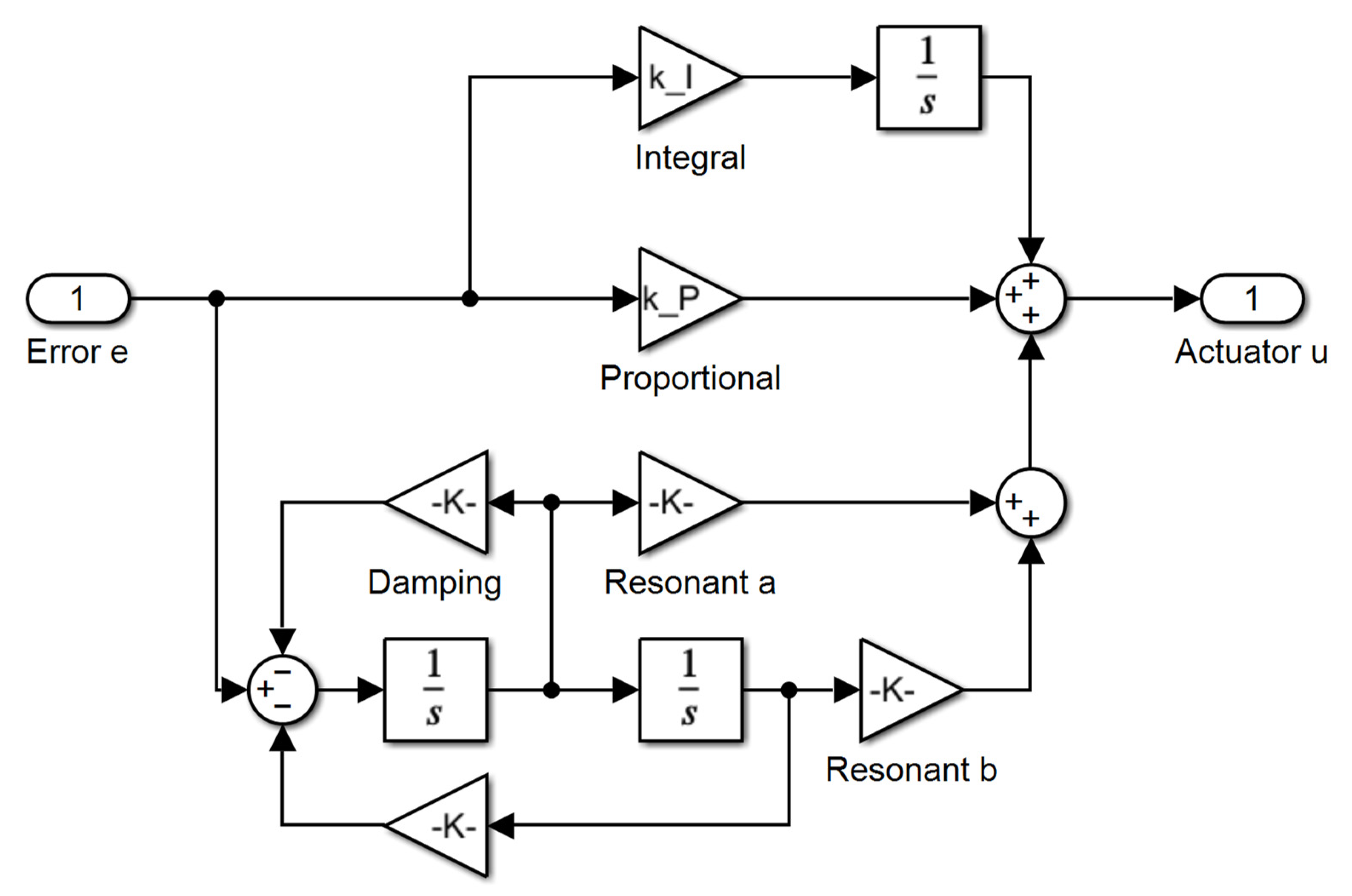
Figure 2.
Structure of a PIR Controller.

Figure 3.
The Control Problem for Mixed Sensitivity Loop Shaping.

Figure 4.
A Modulating Integral Controller.

Figure 5.
The Iterative Learning Control structure.

Figure 6.
Bode Plot of the Mixed Sensitivity Design controller.

Figure 7.
Bode Plot of PIR, PIRA and modulating controller.

Figure 8.
Comparing the Bode Plot of the four controllers.

Figure 9.
Comparing the Bode Plot of the open loop chain for the three controllers.

Figure 10.
Bode Plot of the Closed Loop Sensitivity comparing all three controllers.

Figure 11.
Closed Loop Step Response comparing all three controllers.


Table 1.
Comparison between the different control approaches.
| Control Method | Tuning | Implementation | Stability | Reference Tracking | Ripple Suppression |
|---|---|---|---|---|---|
| PI | Easy | Easy | Excellent | Excellent | None |
| PIR | Hard | Easy | Good | ||
| Mixed Sensitivity | Automated | Easy | Guaranteed | Marginal | Good (adjustable) |
| Modulating | Hard | Medium | Good | ||
| PIRA | Medium | Easy | Excellent | Very Good | Good |
| ILC | TBD | Medium | Tricky | Good | Good |
Publisher’s Note: MDPI stays neutral with regard to jurisdictional claims in published maps and institutional affiliations. |
© 2022 by the authors. Licensee MDPI, Basel, Switzerland. This article is an open access article distributed under the terms and conditions of the Creative Commons Attribution (CC BY) license (https://creativecommons.org/licenses/by/4.0/).
Share and Cite
MDPI and ACS Style
Steffen, T.; Rafaq, M.S.; Midgley, W. Comparing Different Resonant Control Approaches for Torque Ripple Minimisation in Electric Machines. Actuators 2022, 11, 349. https://doi.org/10.3390/act11120349
AMA Style
Steffen T, Rafaq MS, Midgley W. Comparing Different Resonant Control Approaches for Torque Ripple Minimisation in Electric Machines. Actuators. 2022; 11(12):349. https://doi.org/10.3390/act11120349
Chicago/Turabian StyleSteffen, Thomas, Muhammad Saad Rafaq, and Will Midgley. 2022. "Comparing Different Resonant Control Approaches for Torque Ripple Minimisation in Electric Machines" Actuators 11, no. 12: 349. https://doi.org/10.3390/act11120349
Note that from the first issue of 2016, this journal uses article numbers instead of page numbers. See further details here.