Article

Comparative Study of AI-Based Methods—Application of Analyzing Inflow and Infiltration in Sanitary Sewer Subcatchments

1
Department of Geography, Texas A&M University, 3147 TAMU, College Station, TX 77843, USA
2
Department of Built Environment, Aalto University, Otakari 4, 00076 Espoo, Finland
3
Department of Electrical & Computer Engineering, Texas A&M University, 3127 TAMU, College Station, TX 77843, USA
4
Finnish Meteorological Institute, Erik Palménin aukio 1, 00560 Helsinki, Finland
5
Hydraulic Engineering Institute, Dalian University of Technology, No.2 Linggong Road, Ganjingzi District, Dalian 116024, China
6
Department of Civil and Environmental Engineering, University of Illinois at Urbana-Champaign, 205 N Mathews Ave, Urbana, IL 61801, USA
7
Texas A&M AgriLife Center at El Paso, Texas A&M University, 1380 A&M Circle, El Paso, TX 79927, USA
*
Author to whom correspondence should be addressed.
Sustainability 2020, 12(15), 6254; https://doi.org/10.3390/su12156254
Submission received: 7 June 2020 / Revised: 26 July 2020 / Accepted: 31 July 2020 / Published: 3 August 2020

Abstract

:
Inflow and infiltration (I/I) is a common problem in sanitary sewer systems. The I/I rate is also considered to be an important indicator of the operational and structural condition of the sewer system. Situation awareness in sanitary sewer systems requires accurate wastewater-flow information at a fine spatiotemporal scale. This study aims to develop artificial intelligence (AI)-based models (adaptive neurofuzzy inference system (ANFIS) and multilayer perceptron neural network (MLPNN)) and to compare their performance for identifying the potential inflow and infiltration of the sanitary sewer subcatchment of two pumping stations. We tested the performance of these AI models by using data gathered from two pumping stations through a supervisory control and data acquisition (SCADA) system. As a result, these two AI models produced similar inflow and infiltration patterns—both subcatchments experienced inflow and infiltration. On the other hand, the ANFIS had overall higher performance than that of the MLPNN model for modelling the I/I situation for the catchments. The results of the research can be used to support spatial decision making in sewer system maintenance.

1. Introduction

Sewer systems are used to collect sewage from water consumers and convey it to wastewater-treatment plants, forming part of society’s critical infrastructure. In theory, sanitary sewers should only carry sewage originating from water consumption. Dry weather flow should follow the same pattern as water consumption in a physically undamaged, watertight network. Typically, this pattern reaches its minimum at night and has two peaks during the day [1]. In sewer networks, pumping stations divide the network into subcatchments. In modern installations, pumping stations are connected to a control-room environment through the supervisory control and data acquisition (SCADA) system that automatically transfers flow data to the database system. However, extraneous flow resulting from inflow and infiltration (I/I) is a commonly experienced problem in sewer systems. A high I/I level can be an important indicator of the operational and structural condition of a sewer network [2,3]. Infiltration indicates that pipes and manholes have structural deficiencies, whereas inflow implies inadequate runoff management or deficient manhole covers. The identification of I/I sources requires costly and laborious inspections and measurement campaigns, and results are subject to uncertainty.
I/I problems were intensively discussed in the literature [3,4,5]. For instance, the use of synthetic unit hydrographs is a common method for I/I quantification [4,6,7]. Unit hydrography is a popular method to show the temporal change in flow, or discharge, per unit of runoff. It is used to model how the flow of a stream will be affected over time by the addition of one unit of runoff [4,6,7]. A simple synthetic unit hydrograph can be built from one to three triangles that approximate a flow response to rainfall. Many of these methods focused on comparing differences between areas, which were useful for defining them reliably but gave different results in estimating total infiltration volumes [3,4]. Authors in [8] used multilinear modelling and dry weather flows for the quantification of groundwater infiltration and surface-water inflow from dry weather flows. The results of network simulations with interpolated groundwater levels, wastewater-treatment-plant inflow, and river-surface-water levels were combined into a hydrodynamic model. Their methods could differentiate between inflow and infiltration with moderate costs. Moreover, authors in [9] developed a nonlinear regression model that allowed detailed physically based infiltration modelling. Authors in [10] applied a nonlinear base-flow-separation algorithm to estimate the proportion of infiltration in daily inflow to wastewater-treatment plants. Authors in [11] applied partial least squares regression to model sewer flow, where flow data were derived from the wastewater-billing system, and rainfall data were collected from rain gauges. Authors in [12] statistically assessed the performance of rehabilitation measures to reduce inflow and infiltration.
An AI-based approach has not been extensively used in modelling I/I problems. Shehab and Moselhi introduced the automated detection and classification of infiltration in sewer pipes [13]. An AI-based approach was also used in predicting flow to wastewater-treatment plants [14,15] and river-flow prediction [16,17]. The unit-hydrograph method can be applied to estimate the flow response to individual rainfall events, which typically last for minutes rather than hours. However, those methods are hard to implement to predict the I/I rate in real-time. Often, hourly flow data are collected using a SCADA system that contains outliers and systematic errors. The uncertainties of wastewater-flow data cause difficulties in using traditional mathematical approaches, e.g., the partial least squares regression of authors in [11], which demands high degrees of precision and accuracy.
This research aims to develop an AI-based approach for analyzing time-series wastewater-flow data that are collected automatically from the SCADA system in order to predict the I/I rate in real-time. The results of the work can be used to support spatial decision making in sewer system maintenance. Two AI-based models (adaptive neuro-fuzzy inference system (ANFIS) and multilayer perceptron neural network (MLPNN)) were developed for identifying the I/I for the subcatchments of sanitary sewer networks. We tested the performance of these AI models by using data gathered from two pumping stations of the city of Espoo in Finland. The ANFIS uses hybrid learning algorithms to map an input space to an output space, which captures the nonlinear and uncertain relationships of the dataset [18]. The ANFIS represents one of the AI models that was used in predicting river-water levels and discharge, groundwater-inflow rate, rainfall runoff, and water-piping networks [19,20,21,22]. The ANFIS has also been used for real-time data analysis and data fusion [23]. Artificial neural networks are the most well-known approach for building robust nonlinear models and has advantages, including the ability to capture the nonlinear structure of a process, adaptation capability, and rapid learning capacity [24]. In the present investigation, we used the MLPNN algorithm that has a standard structure: input, one hidden, and one output layer, and was reported in the literature as a universal approximator [25,26,27]. There are several advantages of using MLPNN artificial neural networks [25,26,27]. It is data-driven that do not require any restrictive assumptions on the form of the model. On the other hand, the model has the ability to generalize, thus the neural networks will respond to new data that has not been used in the training phase. The MLPNN is able to detect complex nonlinear relationships between variables. The ANFIS model has often been compared with the MLPNN algorithm in the application areas of modelling river temperature and water-quality management [28,29]. Compared to artificial neural networks (ANNs), the ANFIS model is more transparent to the user and causes fewer memorization errors [28,29].
The rest of the article is organized as follows: Section 2 gives an overview of the study area, datasets, and theoretical background that is relevant to the development of the AI-based models. Section 3 illustrates the results and validation of both models. The discussion and conclusion are presented in Section 4 and Section 5, respectively.

2. Materials and Methods
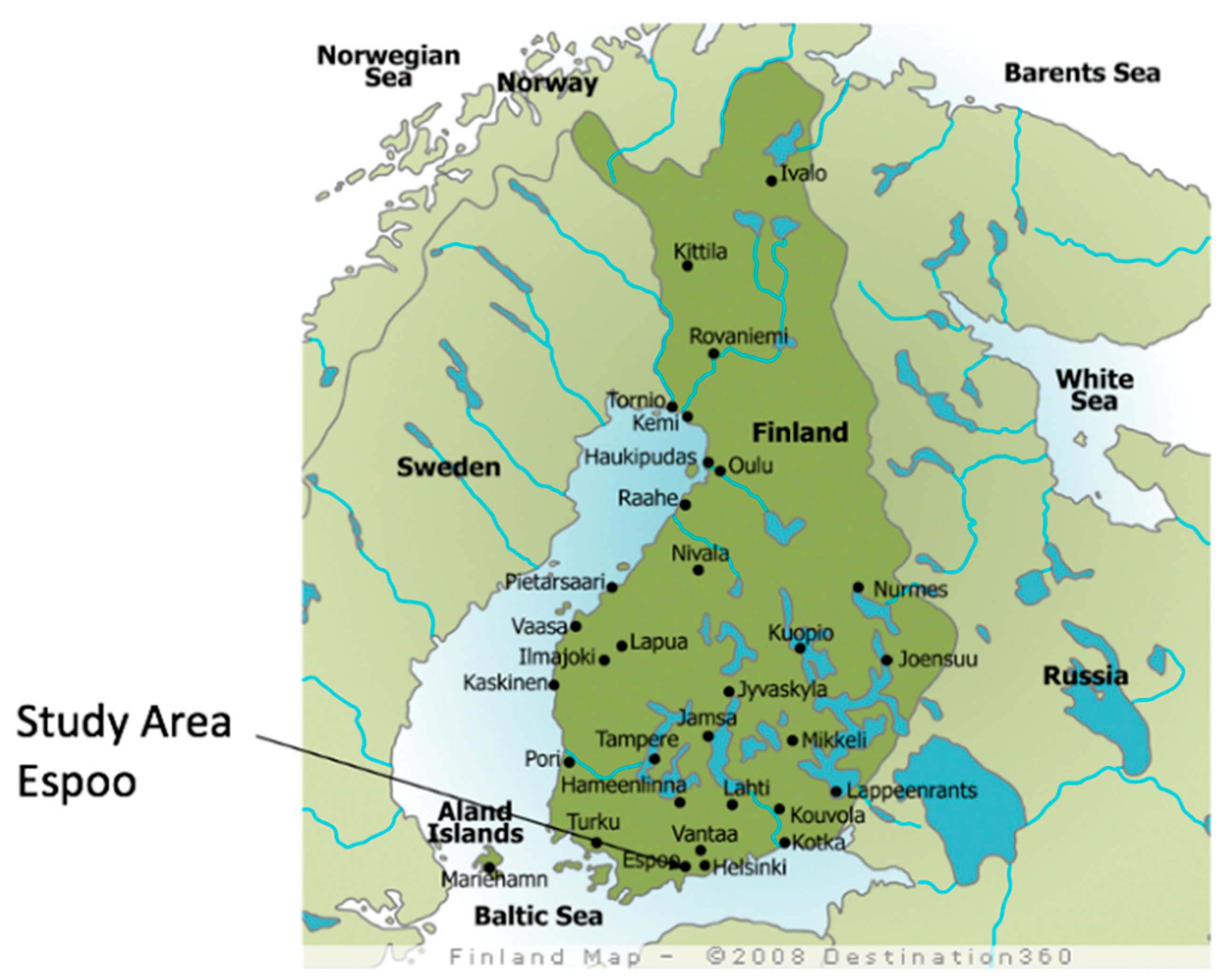
2.1. Study Area

The study area was in the city of Espoo, Finland (Figure 1). The Espoo sanitary sewer network is more than 900 km long and contains approximately 200 pumping stations. A subcatchment is defined as a surface area that potentially contributes rainfall-induced runoff to the flow at a pumping station. Subcatchments were delineated by using a watershed algorithm. The flow-direction raster was generated by using the eight-direction flow model and the 2 × 2 m digital elevation model (DEM) provided by the National Land Survey of Finland. The sewer network was burnt into the elevation model so that the direction of flow in a sewer was correct and rainfall could flow into a sewer system. After that, each subcatchment that contributes the surface runoff to another pumping station was excluded. All network pipes located upstream of a pumping station were rasterized and used as pour point cells in the watershed algorithm. The first subcatchment has an area of 1.1 km2, and the second subcatchment has an area of 0.7 km2.

2.2. Data Collection and Processing

We used radar-based rainfall measurement in this study since the Espoo area has only two rain gauge sites, but radar measurements cover all study catchments. Rainfall data were obtained from the Vantaa C-band dual-polarization radar operated by the Finnish Meteorological Institute (FMI) [30,31]. Weather-radar data had high spatial (100 × 100 m) and temporal (five minutes between each scan) resolution. Two preprocessing steps were carried out to avoid contamination of radar measurements by the ground clutter, which was a considerable issue at close range (<30 km from the radar). For each elevation angle, the radar data was first resampled to a 100 × 100 m horizontal grid using inverse distance-weighted interpolation. The resulting grids were vertically interpolated to a constant altitude level of 500 m in the second stage. This was done by linear interpolation between the two radar scans nearest to the 500 m level.
The removal of non-meteorological echoes and filling the resulting gaps in the radar data were performed by using the AnDRe software package, which is in operational use at the FMI [32]. Reflectivity measurements from six elevation angles were combined by interpolating them to a constant altitude level of 500 m. For the conversion of radar reflectivity (Z) into rainfall intensities (R), the Z–R relationship adapted to the Finnish climate was used, where Z is in units of millimeters to the sixth power per cubic meter, and R is in millimeters per hour [33].
Z = 223 × R 1.53
Rainfall intensities were interpolated into a 100 × 100 m grid enclosing each catchment. The final rainfall data were available in an hourly scale. Hourly rainfall accumulations were then obtained by averaging intensities measured every five minutes. Finally, rainfall accumulations were bias corrected by using two rain gauges located in the Espoo area. The correction factors were separately estimated for each year in the dataset.
Wastewater-flow data were collected from four to seven snowless months for each year from 2012 to 2014, altogether covering 17 months of time-series wastewater-flow data. The data-collection period was selected to make sure that frost and snowmelt did not falsify the results. Hourly follow data received from two pumping stations were used for analysis, and SCAD- based flow data quality was found to be adequate. At the pumping stations, flow data were estimated by using the registered number of times that a pump well was emptied in an hour multiplied by the well volume. After that, the SCADA system sent this information to a control room. In the data pre-processing phase, obvious errors of the dataset were removed. These two subcatchments did not experience sewer overflows within the data-collection period, which ensured the flow dataset that captures a typical inflow and infiltration response to a rainfall event.
In this study, three rainfall-threshold values were defined. According to the definition provided by FMI, a dry day is a day in which the amount of rainfall is less than 0.3 mm/day, and a rainy (wet) day refers to a day in which the total amount of rainfall varies from 1 to 4.4 mm/day [30]. According to the definition, three rainfall-threshold values, 0.3, 1, and 2 mm/day, were defined. After that, the amount of rainfall-threshold value was further divided by 24 h to obtain the estimated hourly rainfall value. For each pumping station, the flow dataset was divided into dry- and wet-day datasets according to three rainfall-threshold values. The data that had a lower value than the threshold value formulated a dry-weather dataset, and the rest were considered as the wet-weather dataset. After that, each dataset was normalized and used for both AI-based models. Table 1 illustrate the input and output variables for the ANFIS and MLPNN models.

2.3. Water Consumption in Study Areas

Water-consumption variations need to be considered when studying I/I since water consumption becomes the main component in sewer base flow. In this research, water-consumption data are available for both subcatchment areas for each quarter of the year from 2012 to 2014 and were estimated on the basis of water-consumption billing information. The water consumption of Subcatchments 1 and 2 was 36,000 and 62,000 m3/year, respectively. Analysis results showed that, from April to June and from July to September, water consumption was approximately 1.2% and 0.4%, respectively, less than the whole-year average, which indicated that annual variation in water consumption has little effect on the sewer base flow.

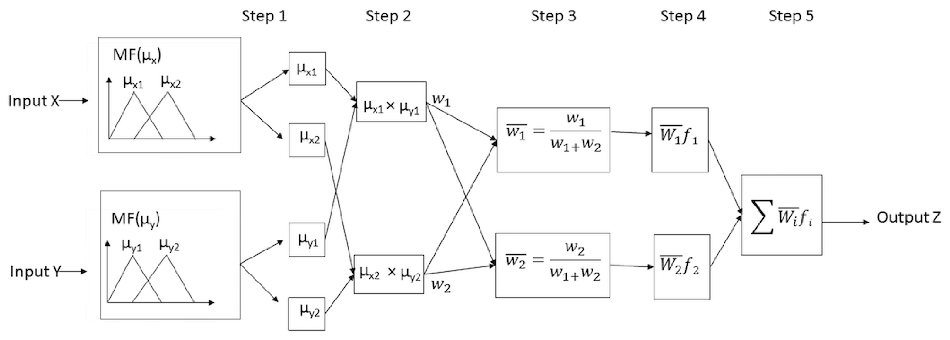
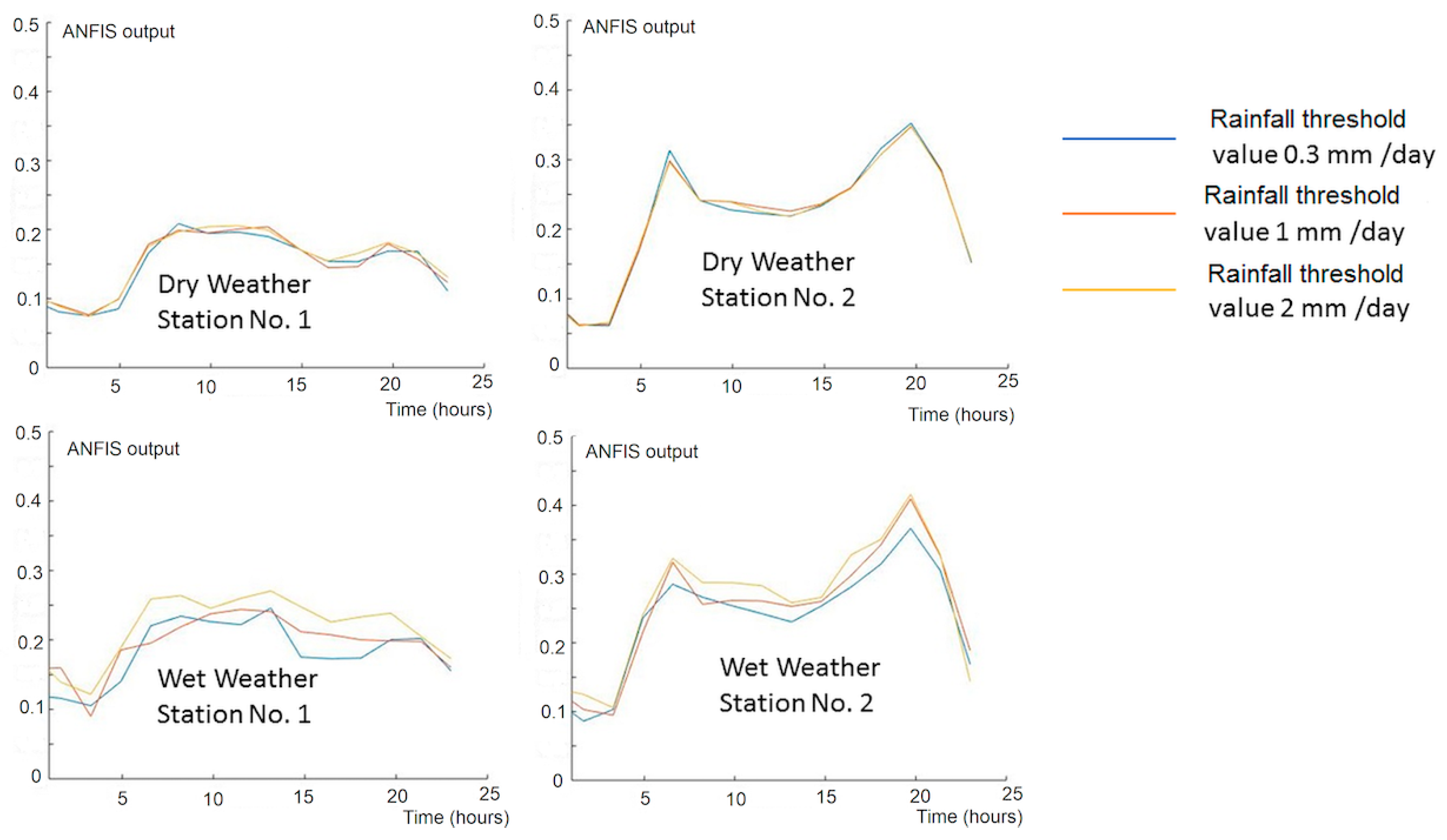
2.4. Adaptive Neurofuzzy Inference System (ANFIS)

Fuzzy-set theory was first introduced by Zadeh as a mathematical theory of vagueness [34]. If X is the universe of discourse, and its elements are denoted by x, then fuzzy set A in X is defined as a set of ordered pairs called the membership functions (MFs) of x in A. The fuzzy set maps each element of X to an MF value between 0 and 1. The degree of membership function µx is used to measure the degree to which the input variable belongs to different MFs. For instance, input value x more likely belongs to a low MF than a medium MF if the value of µx(low) is greater than that of µx(middle). Fuzzy rules, such as “if input X is low and input Y is medium, then output Z is low,” are then used to obtain the relationship between input and output. Fuzzy operators OR, AND, and NOT in the fuzzy rule can be used to describe a fuzzy union, intersect, or complement operations of the input MFs. For instance, a Gaussian function depends on two parameters, σ and c, as given by
f ( x ;   σ , c ) = e ( x c ) 2 2 σ 2
The author in [35] introduced the ANFIS principles. Figure 2 illustrates a general ANFIS architecture using five steps [35]. In the first step, input variables X and Y are specified, and each input variable is described by using two MFs. In this case, two fuzzy rules are created for two input variables, where {ai, bi, ri} is the parameter set (consequent parameters):
Rule 1: If input X is µx1 and input Y is µy1,
then f1 = a1 µx1+b1 µy1+r1
Rule 2: If input X is µx2 and input Y is µy2,
then f2 = a2 µx2+b2 µy2+r2.
In the second step, two elements are created by multiplying the input MFs, and they are used to represent the strength of the rule. In the third step, the strength of the rule is normalized by calculating the ratio of the strength of the ith rule to the sum of the strengths of all the rules. After that, normalized rule strength w i   _ is multiplied by the consequent part of the rule (function f). In the last step, overall output Z is computed by using the sum of all incoming elements.
ANFIS is an adaptive network that consists of nodes and directional links through which nodes are connected. The outputs depend on the parameter(s) pertaining to these nodes, and a learning rule specifies how these parameters should be changed to minimize a prescribed error measure [35]. The ANFIS uses a hybrid learning algorithm [35]. Let us assume that the adaptive network under consideration has only one output.
o u t p u t = F ( I , S ) ,
where I is the set of input variables, and S is the set of parameters. If there is a composite function HF and it is linear in the elements of S, the elements can be identified by using the least squares method [29]. For instance, S can be decomposed into the direct sum of two sets S 1 and S 2 , and function HF is linear in the elements of S 2 .
H ( o u t p u t ) = H     F   ( I , S ) .
Training data P can be plugged into Equation (7). It obtains matrix equation AX = B, where X is an unknown vector whose elements are the parameters in S 2 . A least square estimation (LSE) of X, X * is sought to minimize squared error | | A X B | | 2 , where X * uses a pseudoinverse of X. As a result, sequential formulas are employed to compute the LSE of X. Let the ith element of B be b i T ; then, X can be iteratively calculated using sequential formulas.
X i + 1 = X i + S i + 1 a i + 1 ( b i + 1 T a i + 1 T X i )
S i + 1 = S i S i a i + 1 a i + 1 T S i 1 + a i + 1 T S i a i + 1 ,   i = 0 , 1 , , P 1 ,
where S i is often called the covariance matrix, and least squares estimation X * is equal to X P . For the multioutput adaptive network, b i T is the ith rows of matrix B.
In the ANFIS, each epoch of this hybrid learning procedure is composed of a forward and backward pass. In a forward pass, input data and functional signals go forward to calculate each node output until matrix AX = B is obtained, and parameter S 2 is identified by the sequential least squares formulas (Equations (7) and (8)). After that, functional signals keep going forward until error measures are calculated. In a back pass, error rates propagate from the output end towards the input end, and the parameters in S 1 are updated. Error tolerance is used to create a training stopping criterion that is related to error size. The training stops after the training-data error remains within this tolerance.

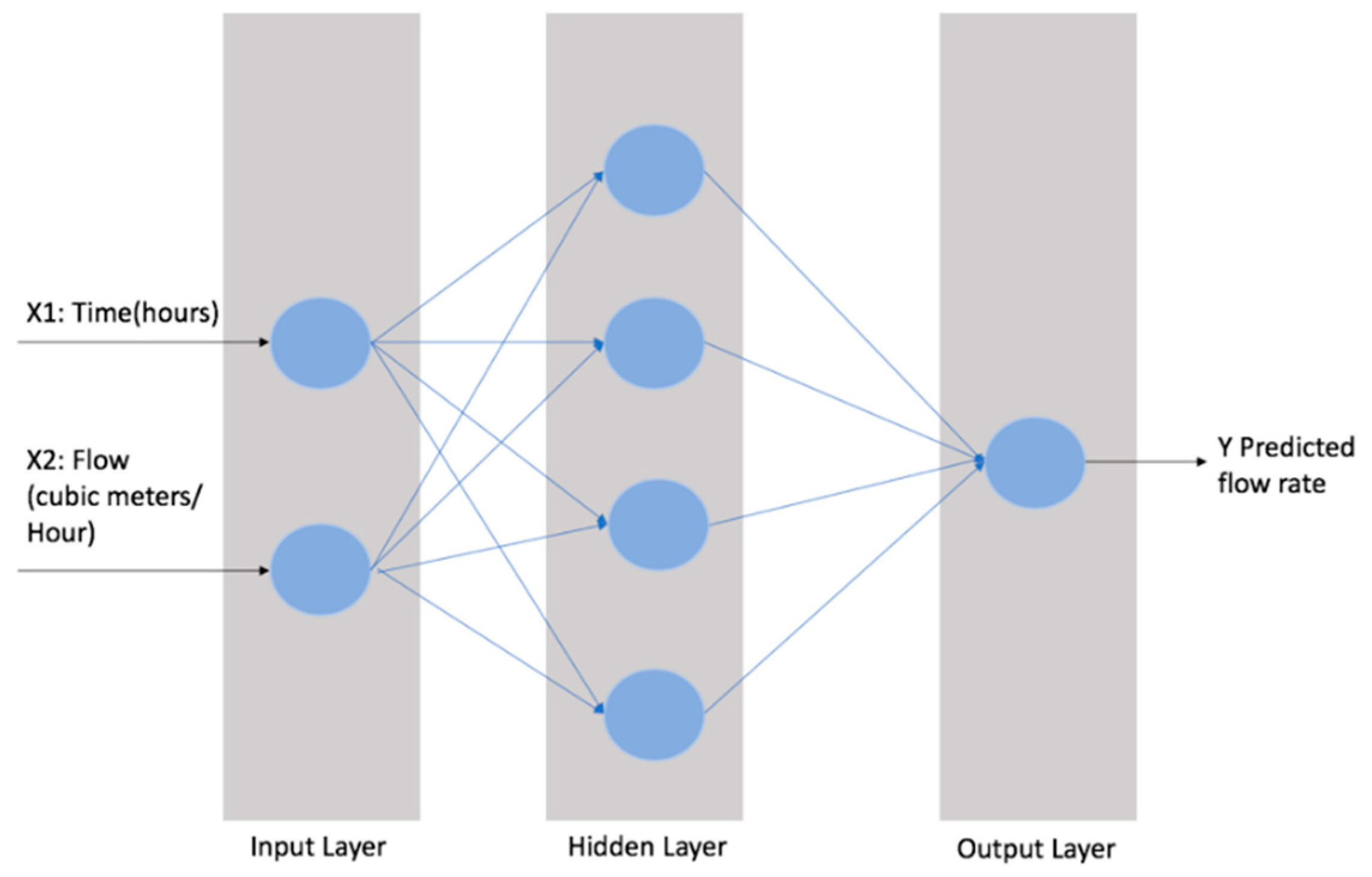
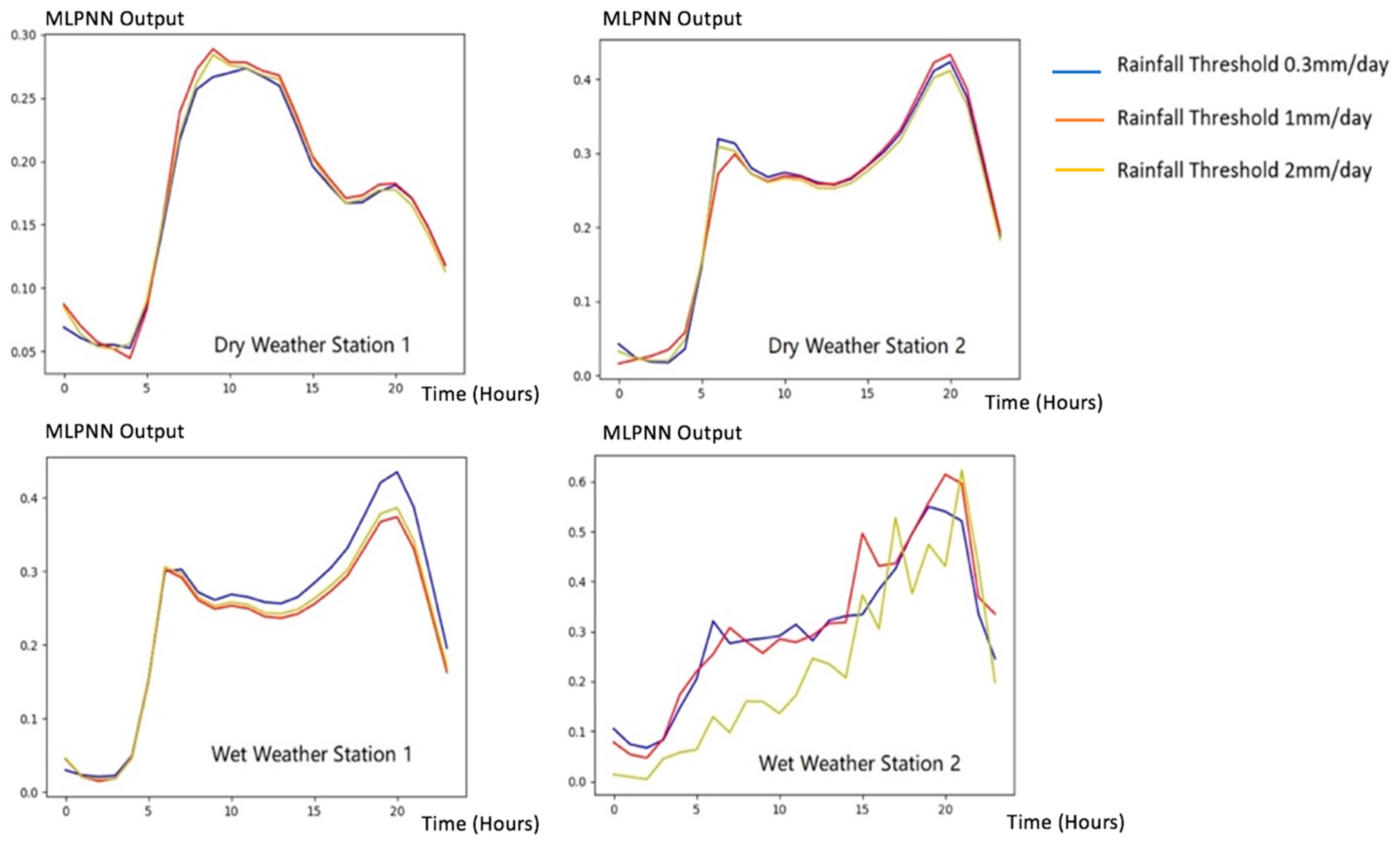
2.5. Multilayer Perceptron Neural Network

Artificial neural networks (ANNs) are a first-order mathematical approximation to the human nervous system that have been widely used for modelling nonlinear models [24]. ANN models are organized in three parallel layers: input, hidden, and output layers. The input layer contains the input variables, and the hidden layer contains several neurons determined using trial and error. In the beginning, neurons in the hidden layer receive input variables multiplied by the corresponding weights to perform a summation. In the second stage, the result is passed to the second layer through a nonlinear activation function, generally the sigmoid. In the output layer, we have only one neuron that corresponds to the dependent variables. Equation (9) illustrates the mathematical formula of the MLPNN, with one hidden layer containing n neurons and one output layer with only one neuron.
Y = f 2 [ j = 1 n w j k [ f 1 ( j = 1 n x i w i j + δ j ) ] + δ 0 ]
where xi is the input variable, wij is the weight between input i and hidden neuron j, δj is the bias of the hidden neuron j, f1 is the activation sigmoid function, wjk is the weight of connection of neuron j in the hidden layer to unique neuron k in the output layer, δ0 is the bias of the output neuron k, and f2 is a linear activation function for the neuron in the output layer. We choose the MLPNN as a comparison because it is common in supervised learning and has been compared with ANFIS in many other applications [28,29]. In this study, the proposed MLPNN has three layers: one input layer, one hidden layer, and one output layer. The general structure of the MLPNN is illustrated in Figure 3. The input layer has two variables: the flow value and its corresponding time in hours, and the output layer value is the predicted wastewater-flow value at its corresponding time in hours.

2.6. Model Evaluation
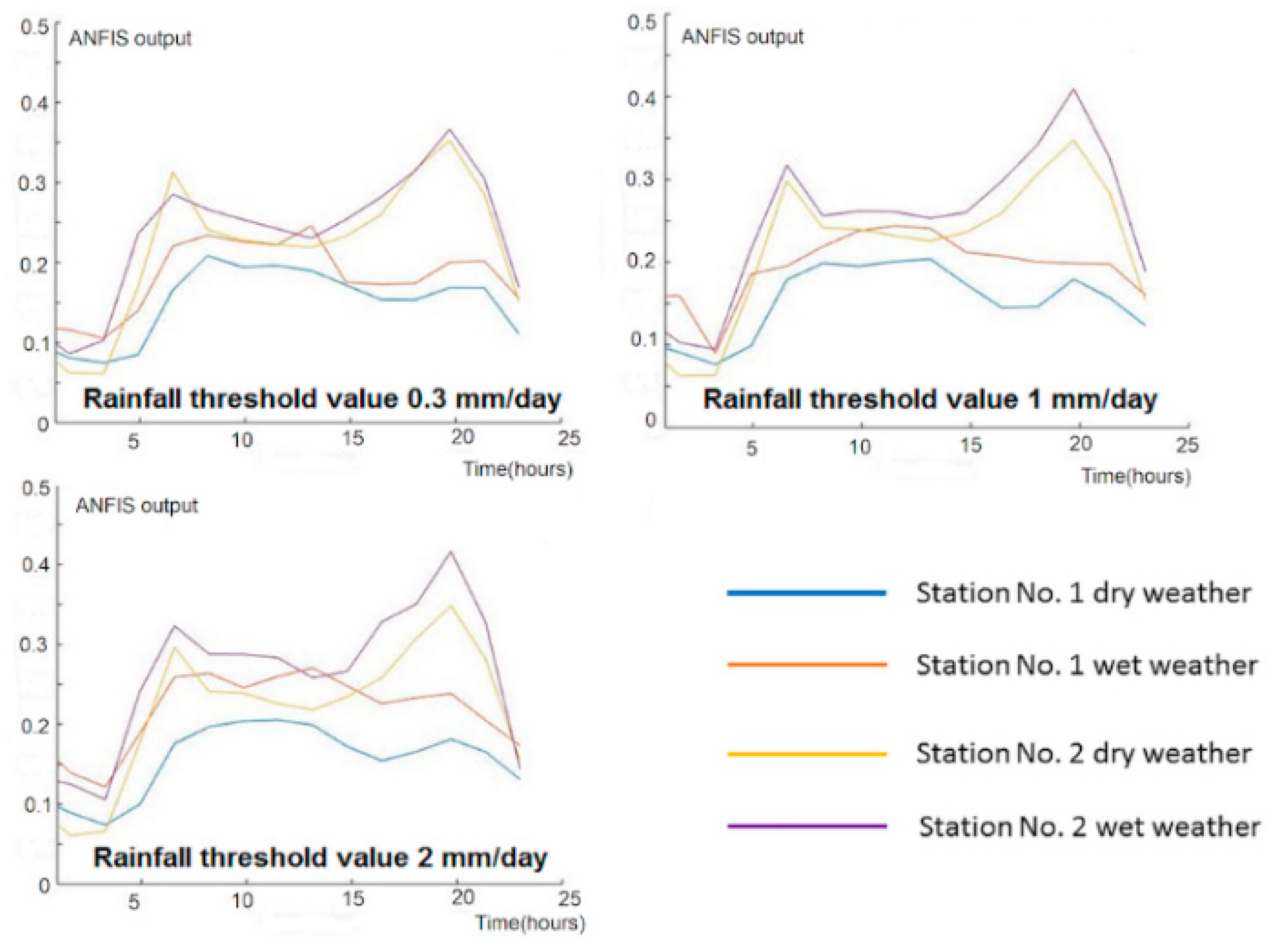
In this study, ANFIS and MLPNN model performance was evaluated using the root mean square error (RMSE) [36] and coefficient of determination (R2). RMSE describes the average difference between experiment values and estimated values, as expressed by Equation (10):
R M S E = 1 N j = 1 N ( y j   y j ^ ) 2 ,
where N is the total number of data pairs, y j is the experiment value, and y j ^ is the estimated value. In the ANFIS, the RMSE method is used to estimate training and checking errors. The training (or checking) error is the difference between a training (or checking)-data output value, and the output of the ANFIS corresponding to the same training (or checking) input value [18]. The training (or checking) error records the RMSE for the training (or checking) data at each epoch. R2 is the coefficient of determination, which is the proportion of the variance in the dependent variable that is predictable from the independent variable (see Equation (11)).
R 2 =   1   i ( y i y ^ j ) 2 i ( y i y ¯ ) 2
In the MLPNN model, RMSE is often used to define the network error. The weights (wij) and bias levels (δ0) (see Equation (9)) are free parameters that can be adjusted when the structure of the neural network is defined. They need to be adjusted in order to minimize the RMSE. Data normalization is an important step in modelling the I/I rate with the MLPNN model. It removes dimensional differences in the data and improves the prediction ability of the MLPNN model. In this study, all variables were normalized using min–max feature scaling, which bring all values into the range from zero to one [37].

3. Results

In the ANFIS model, a parameterized model structure of membership functions and rules were generated, and eight Gaussian MFs were created for each training process. The number of MFs were chosen in such a way that training and checking error could be obtained to an adequate limit. The grid-partition method was used to generate the fuzzy-inference system. In the grid-partition method, a dataset is divided into rectangular subspaces using axis-paralleled partition based on a predefined number of MFs and their corresponding types in each dimension. The number of fuzzy rules increases exponentially when the number of input variables increases; therefore, a grid-partition method is especially suitable for a case with small numbers of input variables. A hybrid learning algorithm was used to train the fuzzy-inference-system (FIS) model, and zero error tolerance was used as a criterion for stopping the training. The training process stops whenever the maximal epoch number is reached, and the training error goal is achieved. In the next step, we trained the MLPNN regressor and fit the model with existing datasets. Finally, the ANFIS and MLPNN models were validated by computing RMSE and R2. The model-evaluation results are illustrated in Table 2 and Table 3. ANFIS had much better RMSE value than the MLPNN model for almost all input datasets except for the wet-weather scenario of the Station 2. For the ANFIS model, the RMSE value is within the range of 0.07 to 0.1199, which is reasonably good. Table 3 also indicates similar results. The ANFIS has better R2 performance than the MLPNN model except for Station 2 dry-weather scenario with a threshold value of 2 mml.
The results of the trained ANFIS and MLPNN models for Subcatchments 1 and 2 are illustrated in Figure 4 and Figure 5. The time in hours is presented on the x-axis and the corresponding models’ output on the y-axis. Models for dry weather flow for pumping Stations 1 and 2 are presented with blue and yellow curves and those for wet weather flow with red and purple curves. Areas between red and blue curves represent the amount of inflow within Subcatchment 1. The area between purple and yellow curves represents the amount of inflow within Subcatchment 2. The curves for different subcatchments were plotted together in Figure 4 and Figure 5, which allowed the inflow levels of the two stations to be compared. Later, the curves of each pumping station for three rainfall-threshold values were plotted to observe the sensitivity of the model towards a change of rainfall-threshold values.
According to Figure 4, both subcatchments experienced inflow, since the wet-weather curve was above the dry-weather curve for most of the time. Subcatchment 1 experienced higher levels of inflow than those of Subcatchment 2. Some exceptions occurred between 15:00 and 20:00, with a rainfall-threshold value of 0.3 and 1 mm/day for the ANFIS model. In addition, inflow value increased for both subcatchments when rainfall-threshold value rose. For instance, Subcatchment 1 suffered from inflow even under mild rainfall with a threshold of 0.3 mm/day, and the two curves were further apart from each other. With a threshold value of 2 mm/day, the difference was even more evident, which indicated that the amount of flow inside the sewer network increased significantly under heavy rainfall.
In addition to inflow, the effect of infiltration can also be identified by studying the minimal night-time flow levels of the subcatchments. For each ANFIS model, input-flow values were normalized; therefore, minimal night-time flow should be the same (normalized value of zero) for both dry- and wet-weather scenarios in an ideal case without infiltration. Night-time minimal flow represents a period of minimal sanitary flow. A high percentage of night-time minimal flow may be attributed to groundwater infiltration [31]. However, for both subcatchments, the flow is always above the zero level, which indicated that the flow is typically above the minimal flow value. If hourly flow data covered only a short period, elevated minimal night-time flows could be caused by atypical water consumption occurring by chance during the studied period. However, the period of data used in the study was relatively long, 17 months in total. Therefore, frequent night-time flow values above the minimum could not be caused by unusual water consumption but by infiltration since these two subcatchment areas are mainly residential areas without big industrial consumers. The ANFIS output values for minimal night-time flow were around 0.07 and 0.06 for Subcatchments 1 and 2, respectively. The infiltration ratio during maximal flow conditions could be calculated by dividing the maximal dry weather flow value by the minimal dry weather night-time flow value. Using the 1 mm/day threshold value, Subcatchments 1 and 2 had infiltration ratios of approximately 40% and 17%, respectively.
Figure 5 illustrates the results of the MLPNN model. The MLPNN model produced a similar pattern as that of the ANFIS model. There were peak values identified in the morning and in the evening. The wet curves were mostly above the dry curves for both stations, which indicated the possibility of having inflow and infiltration. However, curves produced by the MLPNN model seemed to fluctuate since the initial curve of the perceptron model was random, and it needed a larger dataset to teach itself to come to a convergence. If there were no existing data points to calibrate the random value, the value in the results could be far from the expected value, which would generate excessive fluctuation.
In this research work, flow data for typical weekdays were used to ensure that water-consumption behavior in the study area was always similar. According to Figure 4 (rainfall-threshold value 0.3 mm/day), minimal flow occurred around 03:00, flow started to increase rapidly and reached its peak value at around 07:00, and another peak value appeared at around 20:00. This indicates that most people living inside the catchment area use more water around 7:00 before leaving to work or school, and 20:00 before going to sleep. Subcatchments of both pumping stations were relatively small, therefore the time needed for flow to reach the pumping station from the farthest reaches of the network was in the order of minutes. Therefore, flow delay would not affect the results.
Figure 6 and Figure 7 illustrate sensitivity analysis of the ANFIS and MLPNN models to a change of rainfall-threshold values. Results showed that both models were not sensitive to a change of the threshold value in the dry-weather scenario but sensitive in the wet-weather scenario. The reason is that the wet-weather dataset contained much fewer data compared to the dry-weather dataset. When the threshold value increased, the amount of rain data decreased rapidly, which caused the model to be sensitive to the results. Compared to the ANFIS model, the MLPNN model was more sensitive to a change of threshold value for the wet-weather scenario in Station 2. That means that the change of threshold value could make the curve vary more than the ANFIS model. This is because the perceptron model was using random mapping that could exaggerate the difference.

4. Discussion

This article introduced an AI-driven approach to estimate the I/I of two subcatchments. The proposed AI-based models have several advantages in estimating I/I values. A subcatchment is defined as a surface area that potentially contributes to rainfall-induced runoff to the flow at a pumping station. It enables a spatial-thinking approach of the I/I problem and helps to identify locations where sewer maintenance is needed. Therefore, the results of the study can be used to support spatial decision-making for sewer system maintenance. The ANFIS brings better performance than ANN model in predicting the inflow and infiltration of subcatchments. For instance, it is possible to use hourly flow data that include outliers and uncertainties since the ANFIS captures the typical pattern of the majority of data values. On the other hand, the ANFIS cannot be used to estimate inflow and infiltration under extreme conditions since extremely high- and low-flow data points were relatively few and not captured in the ANFIS model.
We used radar-based rainfall measurements in this study to define the sewer subcatchments. There are two types of uncertainty in radar-based rainfall measurements. Systematic biases can happen due to radar calibration issues, wet random attenuation, or a reflectivity-rain rate conversion that is not appropriate to the present weather situation. These can lead to over/underestimation of rainfall over the whole catchment area. If the radar data is gauge-corrected, the systematic biases are not expected to last for a long time period. Random errors can occur at individual locations inside the catchment grid. These can be, for instance, due to ground clutter, beam blockage or attenuation of the radar beam. In addition, note that the bias correction of radar data by rain gauges is not guaranteed to remove all errors. A yearly correction factor using two rain gauges might not be sufficient for correcting transient errors, errors that occur on a very small scale, or errors that occur far from the gauge sites.
In this research, the studied subcatchments were relatively small, thus the time that the flow took from the farthest reaches of the network to reach the pumping station was short (within an hour). In the future, maximal flow delay (e.g., more than an hour) should be incorporated into the model process to make this data-driven approach suitable for different subcatchment sizes. Furthermore, groundwater infiltration was not considered in this research due to the lack of a groundwater-level dataset. If a subcatchment experiences constant groundwater infiltration, e.g., pipes being continuously below the groundwater table, this data-driven approach cannot differentiate between actual sewage flow and groundwater infiltration. In the future, this problem can be solved, e.g., by comparing the groundwater level to pipe locations and finding locations that have a high probability of groundwater infiltration.
We also applied a perceptron neural network model. However, we found that this model had lower performance than the ANFIS, and several problems may exist. First, the perceptron model needs randomly generated datasets, and this can much increase fluctuations. The result was not stable when comparing while calculating multiple times. This would have significantly larger fluctuations when using a small dataset. In the future, other types of machine learning models such as long short-term memory (LSTM) can also be used to conduct time-series analysis of the wastewater-flow data.
One of the objectives of this research work was to use flow data that were automatically collected from pumping stations to analyze the I/I. This entire analysis could be automated in the future since installations that are needed for collecting flow data at pumping stations are already in place. Flow estimation was originally meant to serve automation at pumping stations; therefore, the quality is not yet sufficient for the quantification of I/I in all situations. In the future, after the quality of the flow data has improved, there will be better chances of also estimating the response of the network to individual rainfall events.

5. Conclusions

In this article, two AI-based methods (ANFIS and MLPNN) were developed to incorporate an hourly flow dataset derived from sanitary sewer pumping stations to aid in I/I estimation and sanitary-sewer-system maintenance. Results were validated by computing the RSME and R2 value for each model’s results. The fuzzy model had an overall higher performance than that of the MLPNN model. In this research, three rainfall-threshold values were used to analyze the sensitivity of the model. Using a different threshold value only slightly affected dry-weather curves but significantly affected wet-weather curves. Results indicated that both subcatchments suffered from both inflow and infiltration, and Subcatchment 1 had a higher inflow level than that of Subcatchment 2.
The effect of infiltration could be identified by studying the minimal dry weather flow levels of each subcatchment. The normalized minimal dry weather flows were above zero, which indicated that minimal dry weather flow is typically higher than the flow that is caused by water consumption alone. Therefore, both subcatchments experienced infiltration, and Subcatchment 1 to a higher degree. According to the results, it is recommended that additional studies should be carried out for Subcatchment 1 to further identify the causes for the high levels of both inflow and infiltration.

Author Contributions

Z.Z.; conceptualization, data curation, investigation, methodology, project administration, software development, supervision, visualization, writing original draft, and reviewing and editing; T.L.: data curation, writing original draft, and reviewing and editing; Z.W.: software development, writing original draft, and reviewing and editing; S.P.: data curation, writing original draft, and reviewing and editing; S.A.: data curation, reviewing and editing; K.V.; supervision, reviewing and editing; Y.L.; supervision, reviewing and editing; C.Z.: supervision, reviewing and editing; R.V.: supervision, reviewing and editing; Z.S.: supervision, reviewing and editing; X.C.: reviewing and editing. All authors have read and agreed to the published version of the manuscript.

Funding

This research received no external funding.

Conflicts of Interest

The authors declare no conflict of interest.

References

  1. Tan, P.; Zhou, Y.; Zhang, Y.; Zhu, D.Z.; Zhang, T. Assessment and pathway determination for rainfall-derived inflow and infiltration in sanitary systems: A case study. Urban Water J. 2019, 16, 1–8. [Google Scholar] [CrossRef]
  2. Zhang, Z. Flow data, Inflow/Infiltration Ratio, and Autoregressive Error Models. J. Environ. Eng. 2005, 131, 343–349. [Google Scholar] [CrossRef] [Green Version]
  3. Zhang, M.; Liu, Y.; Cheng, X.; Zhu, D.Z.; Shi, H.; Yuan, Z. Quantifying rainfall-derived inflow and infiltration in sanitary sewer systems based on conductivity monitoring. J. Hydrol. 2018, 558, 174–183. [Google Scholar] [CrossRef] [Green Version]
  4. Yap, H.T.; Ngien, S.K.; Othman, N.; Ghani, A.A.; Abd, N. Preliminary inflow and infiltration study of sewerage systems from two residential areas in Kuantan, Pahang. ESTEEM Acad. J. 2017, 13, 98–106. [Google Scholar]
  5. Wang, X.; Yao, Y.; Zhou, W.; You, L.; Zeng, S. Quantification of Inflow and Infiltration in Urban Sewer Systems Based on Triangle Method. Water Pollut. Treat. 2019, 7, 152–159. [Google Scholar] [CrossRef]
  6. Nasrin, T.; Sharma, A.K.; Muttil, N. Impact of short duration intense rainfall events on sanitary sewer network performance. Water 2017, 9, 225. [Google Scholar] [CrossRef] [Green Version]
  7. Bénédittis, J.D.; Bertrand-Krajewski, J.L. Infiltration in sewer systems: Comparison of measurement methods. Water Sci. Technol. 2005, 52, 219–228. [Google Scholar] [CrossRef] [PubMed]
  8. Karpf, C.; Krebs, P. Quantification of groundwater infiltration and surface water inflows in urban sewer networks based on a multiple model approach. Water Res. 2011, 45, 3129–3136. [Google Scholar] [PubMed]
  9. Karpf, C.; Krebs, P. Modelling of groundwater infiltration into sewer systems. Urban Water J. 2013, 10, 221–229. [Google Scholar] [CrossRef]
  10. Wittenberg, H.; Aksoy, H. Groundwater intrusion into leaky sewer systems. Water Sci. Technol. 2010, 62, 92–98. [Google Scholar] [CrossRef]
  11. Brito, R.S.; Almeida, M.C.; Matos, J.S. Estimating flow data in urban drainage using partial least squares regression. Urban. Water J. 2016, 14, 467–474. [Google Scholar] [CrossRef]
  12. Staufer, P.; Scheidegger, A.; Rieckermann, J. Assessing the performance of sewer rehabilitation on the reduction of infiltration and inflow. Water Res. 2012, 46, 5185–5196. [Google Scholar] [PubMed]
  13. Shehab, T.; Moselhi, O. Automated detection and classification of infiltration in sewer pipes. J. Infrastruct. Syst. 2005, 11, 165–171. [Google Scholar] [CrossRef]
  14. Fernandez, F.J.; Seco, A.; Ferrer, J.; Rodrigo, M.A. Use of neurofuzzy networks to improve wastewater flow-rate forecasting. Environ. Model. Softw. 2009, 24, 686–693. [Google Scholar] [CrossRef]
  15. Haimi, H.; Mulas, M.; Corona, F.; Vahala, R. Data-derived soft-sensors for biological wastewater treatment plants: An overview. Environ. Model. Softw. 2013, 47, 88–107. [Google Scholar] [CrossRef]
  16. Imrie, C.E.; Durucan, S.; Korre, A. River flow prediction using artificial neural networks: Generalisation beyond the calibration range. J. Hydrol. 2000, 233, 138–153. [Google Scholar] [CrossRef]
  17. Fathian, F.; Mehdizadeh, S.; Sales, A.K.; Safari, M.J.S. Hybrid models to improve the monthly river flow prediction: Integrating artificial intelligence and non-linear time series models. J. Hydrol. 2019, 575, 1200–1213. [Google Scholar] [CrossRef]
  18. Zadeh, L.A. Fuzzy Logic Toolbox, for Use with Matlab. Available online: https://www.mathworks.com/help/pdf_doc/fuzzy/fuzzy.pdf (accessed on 6 June 2020).
  19. Alvisi, S.; Franchini, M. Fuzzy neural networks for water level and discharge forecasting with uncertainty. Environ. Model. Softw. 2011, 26, 523–537. [Google Scholar] [CrossRef]
  20. Moghaddasi, M.; Bazzazi, A.A.; Aalianvari, A. Prediction of ground water inflow rate using non-linear multiple regression and ANFIS models: A case study of Amirkabir tunnel in Iran. In Proceedings of the International Black Sea Mining&Tunnelling Symposium, Trabzon, Turkey, 2–4 November 2016. [Google Scholar]
  21. Tsai, M.; Abrahart, R.J.; Mount, N.; Chang, F.J. Including spatial distribution in a data-driven rainfall runoff model to improve reservoir inflow forecasting in Taiwan. Hydrol. Process. 2012, 28, 1055–1070. [Google Scholar] [CrossRef] [Green Version]
  22. Christodoulou, S.; Deligianni, A.; Aslani, P.; Agathokleous, A. Risk-based asset management of water piping networks using neurofuzzy systems. Comput. Environ. Urban Syst. 2009, 33, 138–149. [Google Scholar] [CrossRef]
  23. Kaloop, M.; EI-Diasty, M.; Hu, J. Real-time prediction of water level change using adaptive neuro-fuzzy inference system. Geomat. Nat. Hazards Risk 2017, 8, 1320–1322. [Google Scholar] [CrossRef]
  24. Haykin, S. Neural Networks a Comprehensive Foundation, 2nd ed.; Prentice Hall: Upper Saddle River, NJ, USA, 1994. [Google Scholar]
  25. Zounemat-Kermani, M.; Stephan, D.; Barjenbruch, M.; Hinkelmann, R. Ensemble data mining modeling in corrosion of concrete sewer: A comparative study of network-based (MLPNN & RBFNN) and tree-based (RF, CHAID, & CART) models. Adv. Engin. Inform. 2020, 43, 101030. [Google Scholar]
  26. Hornik, K.; Stinchcombe, M.; White, H. Multilayer feedforward networks are universal approximators. Neural Netw. 1989, 2, 359–366. [Google Scholar] [CrossRef]
  27. Hornik, K. Approximation capabilities of multilayer feedforward networks. Neural Netw. 1991, 4, 251–257. [Google Scholar] [CrossRef]
  28. Zhu, S.; Heddam, S.; Nyarko, E.K.; Hadzima-Nyarko, M.; Piccolroaz, S.; Wu, S. Modeling daily water temperature for rivers: Comparison between adaptive neuro-fuzzy inference systems and artificial neural networks models. Environ. Sci. Pollution Res. 2019, 26, 402–420. [Google Scholar] [CrossRef]
  29. Heddam, S.; Kisi, O.; Sebbar, A.; Houichi, L.; Djemili, L. Predicting water quality indicators from conventional and nonconventional water resources in Algeria country: Adaptive neuro-fuzzy inference systems versus artificial neural networks. In The Handbook of Environmental Chemistry; Springer: Berlin/Hidelberg, Germany, 2019; pp. 1–22. [Google Scholar]
  30. FMI Finnish Meteorological Institute. Sadetta Ja Poutaa. Available online: http://ilmatieteenlaitos.fi/sade (accessed on 6 June 2020).
  31. Saltikoff, E.; Nevvonen, L. First experiences of the operational use of a dual-polarisation weather radar in Finland. Meteorol. Z. 2011, 20, 323–333. [Google Scholar] [CrossRef]
  32. Peura, M. Rack-a program for anomaly detection, product generation, and compositing. In Proceedings of the 7th European Conference on Radar in Meteorology and Hydrology (ERAD 2012), Toulouse, France, 25–29 June 2012. [Google Scholar]
  33. Leinonen, J.; Moisseev, D.; Leskinen, M.; Petersen, W.A.A. Climatology of disdrometer measurements of rainfall in Finland over five years with implications for global radar observations. J. Appl. Meteorol. Climatol. 2014, 51, 392–404. [Google Scholar] [CrossRef] [Green Version]
  34. Zadeh, L.A. Fuzzy sets. Inf. Control. 1965, 8, 338–353. [Google Scholar] [CrossRef] [Green Version]
  35. Jang, J.-S.R. ANFIS: Adaptive-network-based fuzzy inference system. IEEE Trans. Syst. Manag. Cybern. 1993, 23, 665–685. [Google Scholar] [CrossRef]
  36. Chai, T.; Draxler, R.R. Root mean square error (RMSE) or mean absolute error (MAE)?–Arguments against avoiding RMSE in the literature. Geosci. Model Dev. 2014, 7, 1247–1250. [Google Scholar] [CrossRef] [Green Version]
  37. Normalization. Available online: https://en.wikipedia.org/wiki/Normalization_(statistics) (accessed on 6 June 2020).
Figure 1. Illustration of the study area and two subcatchments of pumping stations.
Sustainability 12 06254 g001
Figure 2. General architecture of adaptive neuro-fuzzy inference system (ANFIS) [35].
Sustainability 12 06254 g002
Figure 3. A general framework of the MLPNN model.
Sustainability 12 06254 g003
Figure 4. Trained ANFIS model results by using three rainfall-threshold values.
Sustainability 12 06254 g004
Figure 5. Trained MLPNN model results by using three rainfall-threshold values.
Sustainability 12 06254 g005
Figure 6. Sensitivity analysis of the ANFIS model’s results.
Sustainability 12 06254 g006
Figure 7. Sensitivity analysis of the MLPNN model’s results.
Sustainability 12 06254 g007
Table 1. Input and output variables for the adaptive neurofuzzy inference system (ANFIS) and multilayer perceptron neural network (MLPNN) models.
Input VariablesTime (hours); Wastewater flow rate (cubic meters)
Output VariablePredicted wastewater flow at the corresponding time in hours
Table 2. Illustration of calculated root mean square error (RMSE) for the ANFIS and MLPNN models.
StationsRainfall-Threshold ValuesRMSE ANFISRMSE MLPNN
Station 10.30.0962 (dry weather), 0.1199 (wet weather)0.5328 (dry weather), 0.4272 (wet weather)
10.106 (dry weather), 0.138 (wet weather)0.5247 (dry weather), 0.3334 (wet weather)
20.1035 (dry weather), 0.1492 (wet weather)0.5228 (dry weather), 0.2084 (wet weather)
Station 20.30.076 (dry weather), 0.097 (wet weather)0.3932 (dry weather), 0.3566 (wet weather)
10.0774 (dry weather), 0.1035 (wet weather)0.3932 (dry weather), 0.2495 (wet weather)
20.0775 (dry weather), 0.112 (wet weather)0.3938 (dry weather), 0.1072 (wet weather)
Table 3. Illustration of the calculated coefficient of determination (R2) for the ANFIS and MLPNN models.
StationsRainfall-Threshold ValuesR2 ANFISR2 MLPNN
Station 10.30.8661 (dry weather),
0.8351 (wet weather)
0.6103 (dry weather), 0.6139 (wet weather)
10.8622 (dry weather),
0.8034 (wet weather)
0.5247 (dry weather), 0.4731 (wet weather)
20.8501 (dry weather), 0.6701 (wet weather)0.6092 (dry weather), 0.4565 (wet weather)
Station 20.30.9146 (dry weather), 0.6218 (wet weather)0.7341 (dry weather), 0.5972 (wet weather)
10.9443 (dry weather), 0.5881 (wet weather)0.7273 (dry weather), 0.4472 (wet weather)
20.6678 (dry weather), 0.8765 (wet weather)0.7256 (dry weather), 0.6381 (wet weather)

