Classification of Plant Leaf Diseases Based on Improved Convolutional Neural Network


1
School of Electrical Engineering and Automation, Anhui University, Hefei 230601, China
2
Institutes of Physical Science and Information Technology, Anhui University, Hefei 230601, China
3
School of Electrical and Information Engineering, Anhui University of Technology, Ma’anshan 243032, China
*
Authors to whom correspondence should be addressed.
Sensors 2019, 19(19), 4161; https://doi.org/10.3390/s19194161
Submission received: 28 July 2019
/
Revised: 18 September 2019
/
Accepted: 19 September 2019
/
Published: 25 September 2019
(This article belongs to the Special Issue Advanced Sensors in Agriculture)
Abstract
:Plant leaf diseases are closely related to people’s daily life. Due to the wide variety of diseases, it is not only time-consuming and labor-intensive to identify and classify diseases by artificial eyes, but also easy to be misidentified with having a high error rate. Therefore, we proposed a deep learning-based method to identify and classify plant leaf diseases. The proposed method can take the advantages of the neural network to extract the characteristics of diseased parts, and thus to classify target disease areas. To address the issues of long training convergence time and too-large model parameters, the traditional convolutional neural network was improved by combining a structure of inception module, a squeeze-and-excitation (SE) module and a global pooling layer to identify diseases. Through the Inception structure, the feature data of the convolutional layer were fused in multi-scales to improve the accuracy on the leaf disease dataset. Finally, the global average pooling layer was used instead of the fully connected layer to reduce the number of model parameters. Compared with some traditional convolutional neural networks, our model yielded better performance and achieved an accuracy of 91.7% on the test data set. At the same time, the number of model parameters and training time have also been greatly reduced. The experimental classification on plant leaf diseases indicated that our method is feasible and effective.
1. Introduction
With the rapid development of computer technology, traditional machine learning methods have been applied in plant diseases prediction more and more widely. With the popularity of machine learning algorithms in computer vision, in order to improve the accuracy and speed of diagnostic results, researchers have studied automated plant disease diagnosis based on traditional machine learning algorithms, such as random forest, k-nearest neighbor and support vector machine (SVM) [1,2,3]. Tan et al. established a multi-layer BP neural network model to realize the disease identification of soybean leaves, by calculating the chromaticity values of the leaves [4]. By extracting the color and texture characteristics of grape disease leaves, Tian et al. used a support vector machine (SVM) recognition method which achieved better results than the neural network [5]. Wang et al. developed a discriminant analysis method to identify cucumber lesions, by extracting the color, shape and texture features of leaf lesions, as well as combining with environmental information [6]. Zhang et al. also extracted the color, shape and texture features of lesion after lesion segmentation, and then used them to identify five types of corn leaves by K-nearest neighbor (KNN) classifier [7].
Spraying pesticides is a key step in plant growing. Ron et al. developed a robotic sprayer platform with the collaboration of remote operators for detecting targets and completing spraying tasks. They reported that it can prevent 30% to 35% of crop losses [8]. Autonomous selectivity for spraying pesticides can be used to reduce production costs in agriculture, using an auto-driving robot to detect plants in the crop area and to perform selective injection [9]. Moreover, plant disease detection can be based on spectroscopy and imaging processes. Xie et al. proposed an automatic classifier with multi-level learning features for field crop pests [10]. Sindhuja developed a ground-based sensor system to help monitor the status of plant health and diseases in field conditions [11].
Li et al. proposed an improved deep learning pipeline for automatic localization and count of agricultural crop pests, which integrates a convolutional neural network (CNN) of ZF (Zeiler and Fergus model) and a region proposal network (RPN) with Non-Maximum Suppression (NMS) [12]. Yang et al. proposed a new identification method for rice diseases based on deep convolutional neural networks [13]. The model was trained to identify 10 common rice diseases and tested on a dataset containing 500 natural images of diseased and healthy rice leaves and stems captured from rice fields. Under the 10-fold cross-validation strategy, the CNN-based model achieved an accuracy of 95.48%. Xia et al. proposed a convolutional neural network model to solve the problem of multi-classification of crop insects and achieved a heightened accuracy [14]. Sun et al. proposed an improved convolutional neural network which achieved an accuracy of 99.35% on a test dataset containing 54,306 images, which is composed of 26 diseases in 14 different plants [15]. Moreover, the Pascal VOC (Visual Object Classes) Challenge [16] and the recent ImageNet Large Scale Visual Recognition Challenge (ILSVRC) [17] based on the ImageNet dataset [18], have been widely used as benchmarks for many visualization issues in computer vision, including object classification. In 2012, a convolutional neural network, called AlexNet (Alex’s Network) [19], reduced the top5 error rate of the 1000 categories of classified images to 16.4% on ImageNet.
This work focused on five different convolutional neural network architectures, AlexNet, VGGNet (Visual Geometry Group’s Network) [20], GoogLeNet (Google’s Network) [21], ResNet (Residual Network) [22] and SENet (Squeeze-and-Excitation Network) [23], which participated in ILSVRC from 2012 to 2017, and achieved good classification results. There are still some challenges in plant leaf disease classification, which are as follows:
- (1)
- Limited by experimental conditions, such as current platform and hardware, a large CNN network will cost a long training time and have a slow convergence rate;
- (2)
- Long training convergence time will cause the final classification accuracy to decrease.
To shorten long training convergence time, decrease enormous parameters of most current network models, and increase recognizing accuracy, this paper proposes an integrated method. It adopts the inception structure to fuse the extracted high-level features, the Squeeze-and-Excitation module to perform feature re-calibration for weighting the features in the channel of CNN, and global average pooling instead of the fully connected layer. The experimental results show that our method is effective in the classification and identification of plant leaf diseases. Compared with other traditional convolutional neural networks, our model achieved the highest classification accuracy rate of 91.7% on our plant leaf disease dataset.
2. Materials and Methods
2.1. Data Preprocessing and Augmentation
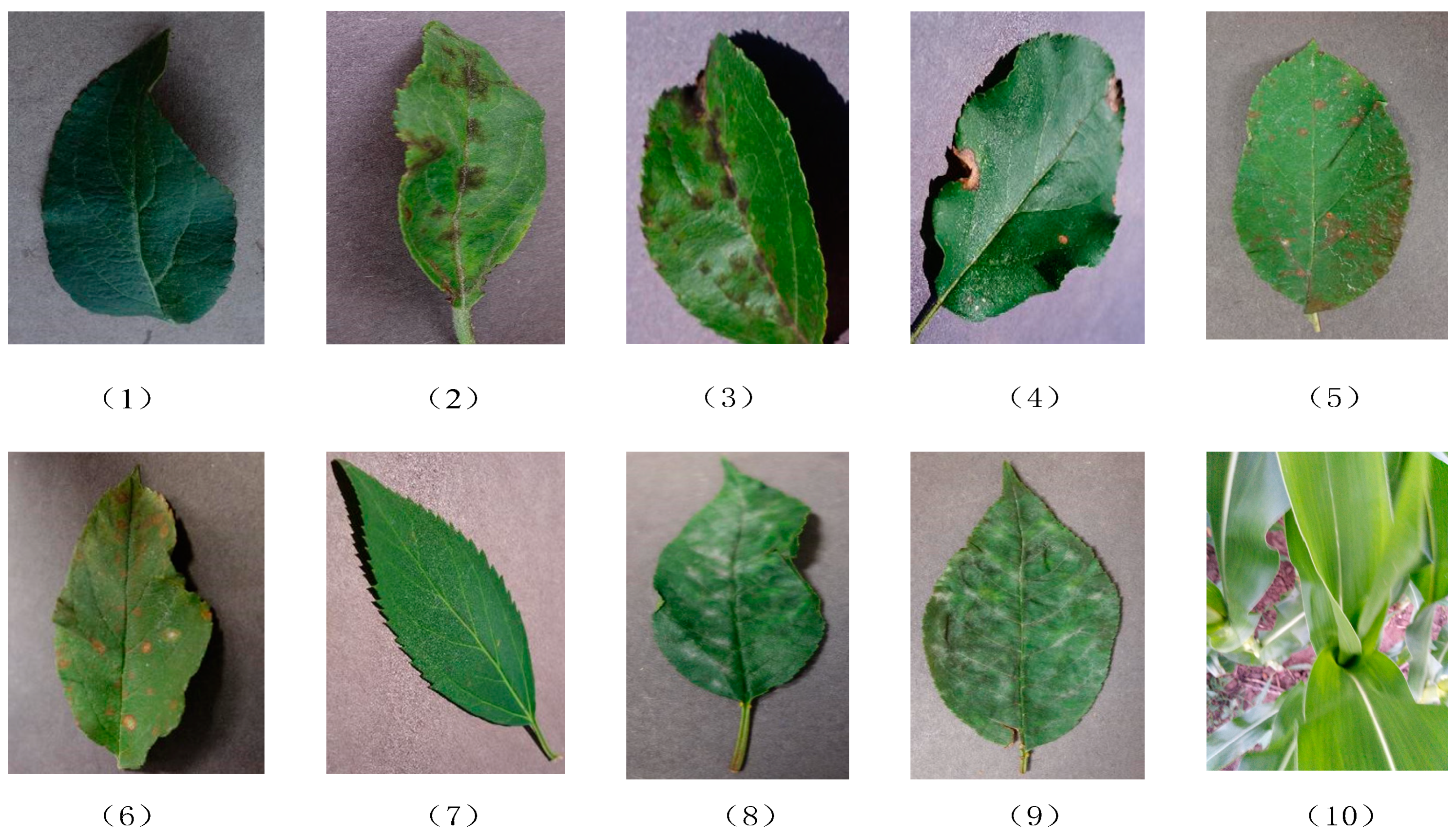
We collected 10 kinds of disease leaf images from a library of plant leaf diseases (https://challenger.ai/), where digital color cameras were used for capturing diseased blade images with a resolution width of 256 and an unfixed length, as shown in Figure 1. Because some types of leaf diseases are confusing and unidentifiable, only 10 types of blade data were selected for our research. As for the images of plant corn, we tried to adopt the image class to verify the identification and showed the generalization ability of different CNN network structures for different types of leaf diseases. The diseased parts of apple and cherry leaves are similar, and the degrees of leaf diseases in different disease levels are also similar. It is more practical for our research. Compared with other types of leaf diseases, these diseased leaves can better reflect the distinguishing ability of disease areas for different CNN structures, and can better compare the ability of different CNN structures in leaf classification.
First, all leaf disease images were adjusted so that the length and width of the image were the same, which were resized to 224 × 224. Resizing images to 224 × 224 before inputting images into different networks is done to adapt different pre-training CNN structures. Then, because some leaf disease types contains less images than others and the collection of leaf disease images are random, images of these disease types were horizontally and vertically flipped. The leaf diseases are Cedar Apple Rust—serious, Cherry Powdery Mildew—general, and Cherry Powdery Mildew—serious. Thus, the leaf disease data set was expanded to prevent redundancy of the data set, ensure the validity of image data, and make the classifier balanced. After the data augmentation, the plant leaf disease dataset contained 6108 images, of which 5588 were for the training set and 520 were for the test set. Table 1 lists the number of images for each disease class.
2.2. Convolutional Neural Network (CNN)-Based Method
2.2.1. CNN Overall Architecture
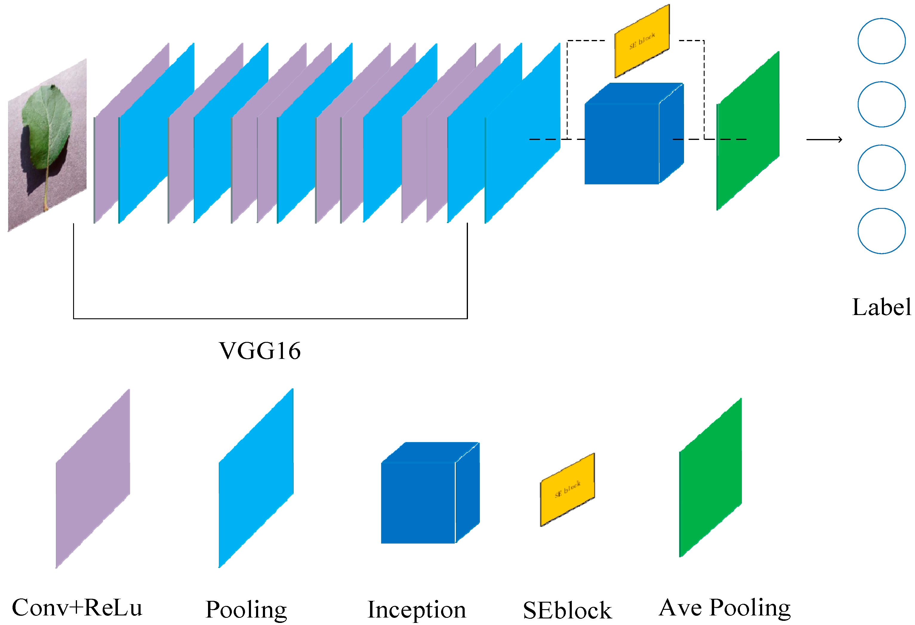
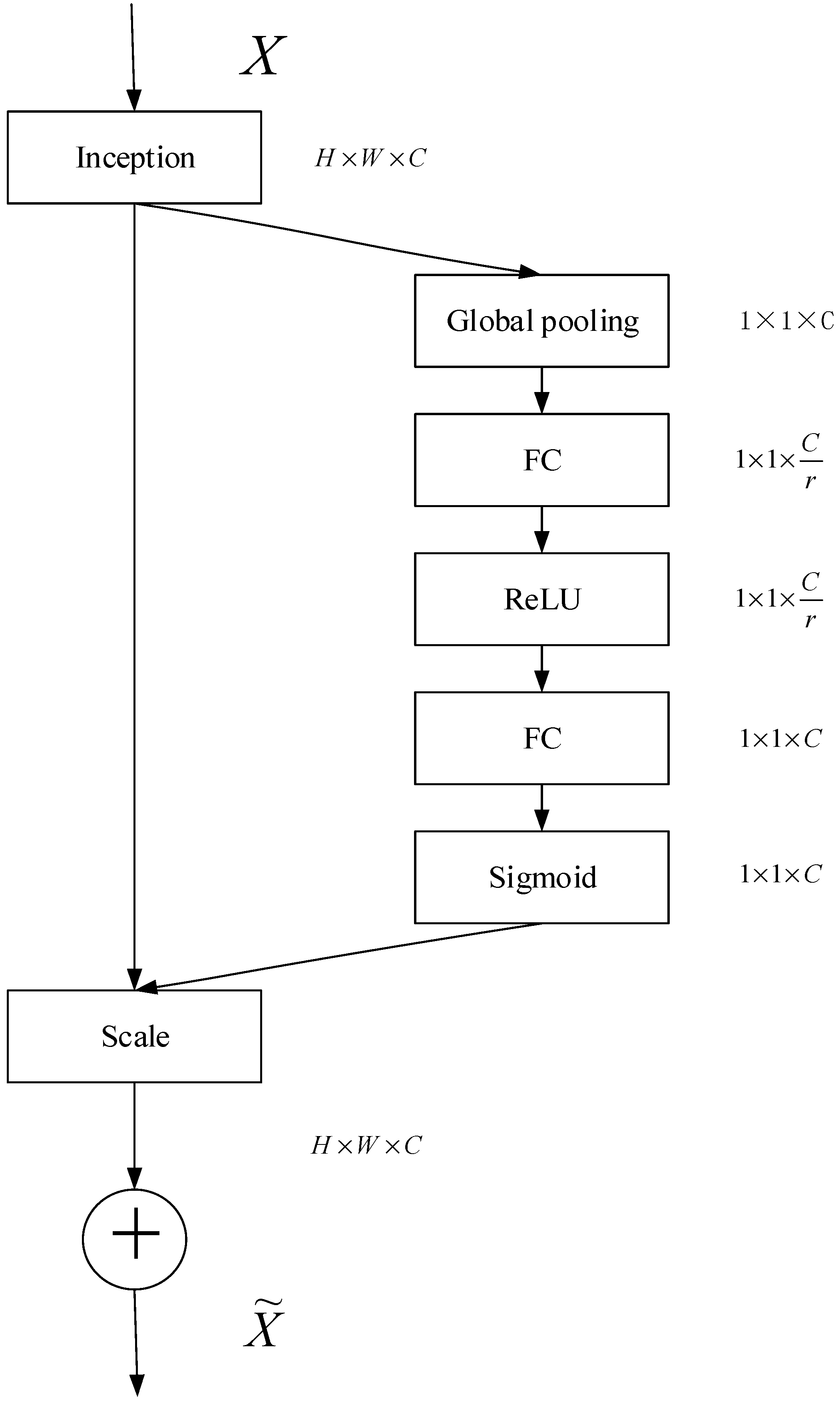
Our deep learning-based network consists of VGG16 convolutional layers as well as the combination of Squeeze-and-Excitation (SE) module and Inception structure. The first five convolutional layers are based on the VGG16 model for self-learning low-to-high features of training images, where deeper convolutional layers reduce more resolution of feature maps, and extract more abstract high-level features. Then, the max pooling layer is used to filter the noise of the feature maps generated by the previous convolutional layer. Inception structure performs feature fusion, broadens the ability of acquiring features on feature maps, and extracts the best distinguishing features based on multi-dimensional analysis. The embedded SE module, re-calibrating the original features in the channel dimension, is used to replace the fully connected layer with the largest average pooling layer, reduce the training parameters as well as quickening the convergence of the model, and thus improving the classification accuracy of the model. The network structure of the improved model and related parameters are shown in Figure 2 and Table 2, respectively.
The five convolutional layers are based on VGG16 pre-training model, which determines which layers of the original network have to be frozen during the pre-training phase, and which layers are allowed to continue learning at a certain learning rate. Usually, the first several layers are frozen because the low-level features can better adapt to various problems. This work used a stochastic gradient descent optimization method to train the model on our own data set. The initial learning rate was set to 0.001, while momentum and weight attenuation were set to 0.0005 and 0.9, respectively. The Dropout layer [24] was used in our experiments to prevent over-fitting in training and make the model more effective.
2.2.2. GoogLeNet’s Inception
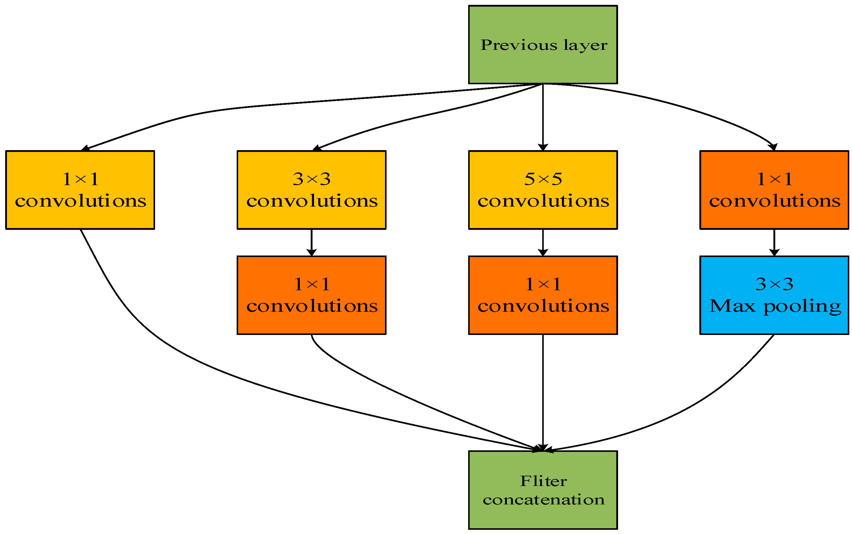
Inception module is the main component of GoogLeNet network. The Inception structure embeds multi-scale information and gathers features from different receptive fields to improve identification performance. It maintains the sparse structure, increases the depth and broadens the width of the network, therefore it reduces not only over-fitting but also free parameters. Figure 3 shows that the Inception module uses three different convolution kernels, 1 × 1 convolution, 3 × 3 convolution, 5 × 5 convolution as well as a 3 × 3 max pooling layer. It extracts three different scale features to increase the diversity of features, involving both macroscopic features and microscopic features. The purpose of the pooling layer is to preserve the primitive input information. The module splices the extracted features in the channel dimension and outputs a multi-scale feature map by concatenating these convolutional and pooling layers together.
2.2.3. Global Average Pooling (GAP)
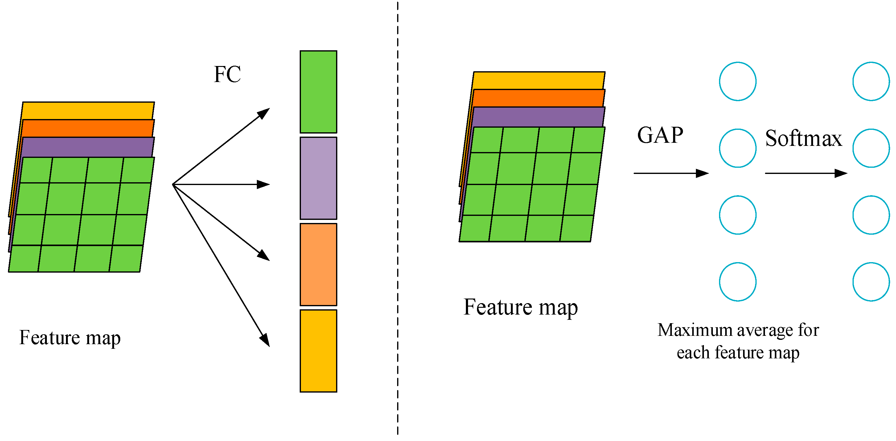
The fully connected network has always been the standard configuration of the CNN network. However, too many parameters in the fully connected layer slows down the training speed of the network and makes it easy to be overfitting. The idea of global average pooling (GAP) [25] is to globally average the entire pixels of each feature map, and get an output for each feature map. The vector that is composed of these output features will be directly sent to softmax for classification. Figure 4 shows the comparison of the fully connected layer and the global averaged pooled layer.
2.2.4. Squeeze-and-Excitation Module
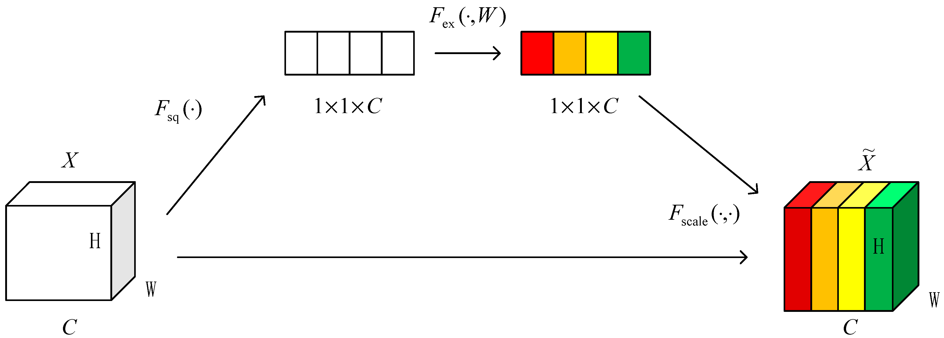
Figure 5 is a schematic diagram of the SE module, which omits the previous series of convolutions in the original SE module. Given an input X, the number of feature channels is C. Unlike the traditional CNN, three operations are taken to recalibrate previously obtained features.
The first one is Squeeze operation. Suppose that the inputs are X = (X1, X2, …, XC), XC ∈ RH×W. Formally, a statistic z ∈ RC is generated by shrinking X through its spatial dimensions H × W. The c-th element of Z is calculated by:
Therefore, the Squeeze operation converts the input of into an output of , corresponding to the Fsq operation in Figure 5. The result of this step is equivalent to the numerical distribution of the C feature maps of the layer, or global information. The output Zc can be thought of as the description of a set of local descriptors for the entire channel map.
The second operation is the Excitation operation. It can represent the convolution and activation operations, which employ a simple gating mechanism with a sigmoid activation:
where, δ refers to the ReLu function, and the output Z can be thought of as a set of local descriptors for the entire channel map, and . In order to control the complexity and generalization of the model, the embedding mechanism of the model is parameterized by two nonlinear fully connected layers.
Finally, a reweight operation regards the weight of the output of Excitation as the importance of each feature channel after feature selection, and then weights previous features by channel weighting to complete the pair in the channel dimension. The output of the block is obtained by rescaling X with the activations s:
where, refers to channel-wise multiplication between the scalar sC and the feature map xC ∈ RH×W, and .
3. Experiments and Results
The experiments were performed on an Ubuntu workstation with CPU i7-8700k and RAM 32G, accelerated by two NVIDIA GTX 1080TI GPUs. All of our experiments were implemented by Caffe, a deep learning open source framework [26]. Moreover, accuracy rate was used to evaluate the performance of network models. The accuracy rate refers to the proportion of the number of corrected positive predictions to that of the whole positive predictions. It can be expressed as:
where, NTP is the number of corrected positive predictions, and NFP is the number of wrongly positive predictions.
3.1. Effects of the Feature Extraction Network
The most important metric we considered is the average accuracy of the test set. Table 3 lists the experimental accuracy, model size and training time for several commonly used deep learning CNN architectures, as well as the results of our method.
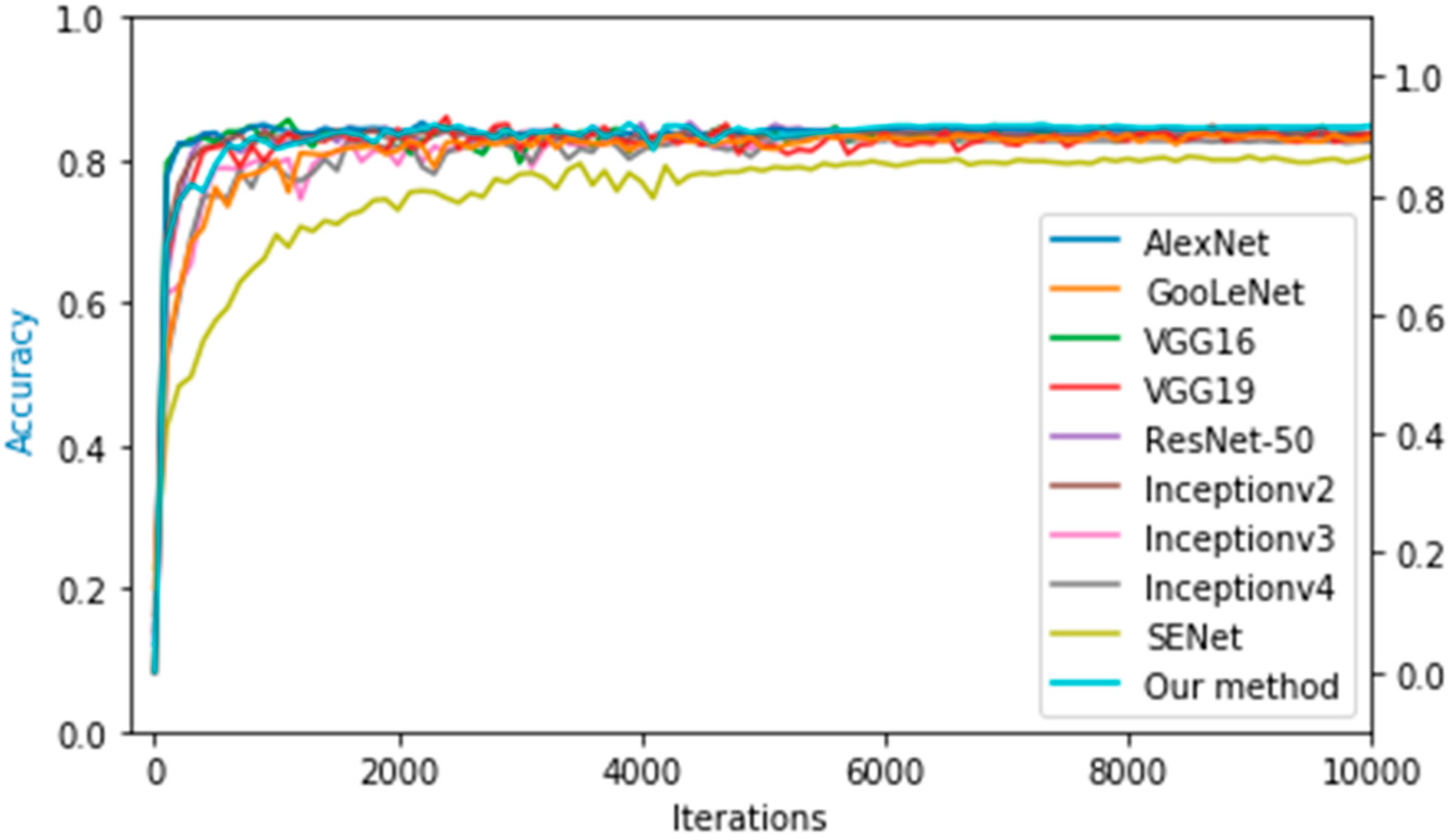
The first observation from Table 3 is that different convolution depths make the trained model produce different classification results on the test set. In general, more convolutional layers can learn more complex features from original images. Shallow CNNs such as AlexNet achieved an accuracy of 0.894 on the test set, while the deep networks VGG16, VGG19, ResNet-50, and Inceptionv2 yielded accuracies of 0.905, 0.903, 0.901 and 0.903 on the test set, respectively. Compared to other networks, our network is relatively shallow, but achieves higher accuracy on the test set. One possible reason is in that shallow network has a relatively good generalization compared to deep ones. The other reason is because of the use of the Inception module to broaden the network and combine the multi-scale feature information, as well as the use of the SE module to merge the feature channel into the Inception module and thus weighted and recalibrated features. As a result, our network achieved a maximum accuracy of 91.7% on the test set. Figure 7 shows the trends of accuracy of different CNN models on the test set.
3.2. Comparison of Model Size for Different Network Models
From the comparison of model size of different models in Table 2, we can get an intuitive observation that the larger the size of the CNN model, the more parameters the CNN had, and the longer the training time. The size of the AlexNet, VGG16, and VGG19 training models were 217 MB, 537.2 MB, and 558.4 MB, respectively. The large model size is because the last three layers of these network structures are all fully connected, which causes the number of the trained network model size to be larger than that of other deep learning models. On the contrary, GoogLeNet, Inceptionv2, and Inceptionv3 with Inception structure greatly reduce the size amount to 47.1 MB, 45.1 MB, and 87.3 MB, respectively. The size of our model is 57.3 MB, which is greatly reduced compared with VGG16 and VGG19. The reason is that our model used the Inception structure and the global average pooling instead of the last three-layer fully connected layer. This structure can avoid the requirement of a large number of weight parameters, reduce the size of the CNN model and solve the problem of large memory occupancy and slow convergence in the training CNN model.
3.3. Comparison of Training Time for Different Network Models
The general CNN model linearly converts all extracted feature maps into 4096-dimensional feature vectors after convolutional and pooled layers, and classifies leaf diseases by softmax layer. Table 4 shows the training time of the forward propagation and backpropagation processes for different CNN models and improved models. As can be seen from Table 4, our model performs a forward propagation rate of 0.038 s, which means that the time required to test a picture is 0.038 s. Compared with other CNN models, our model has a faster advantage in the forward propagation time.
3.4. Loss Function and Confusion Matrix of Our Network
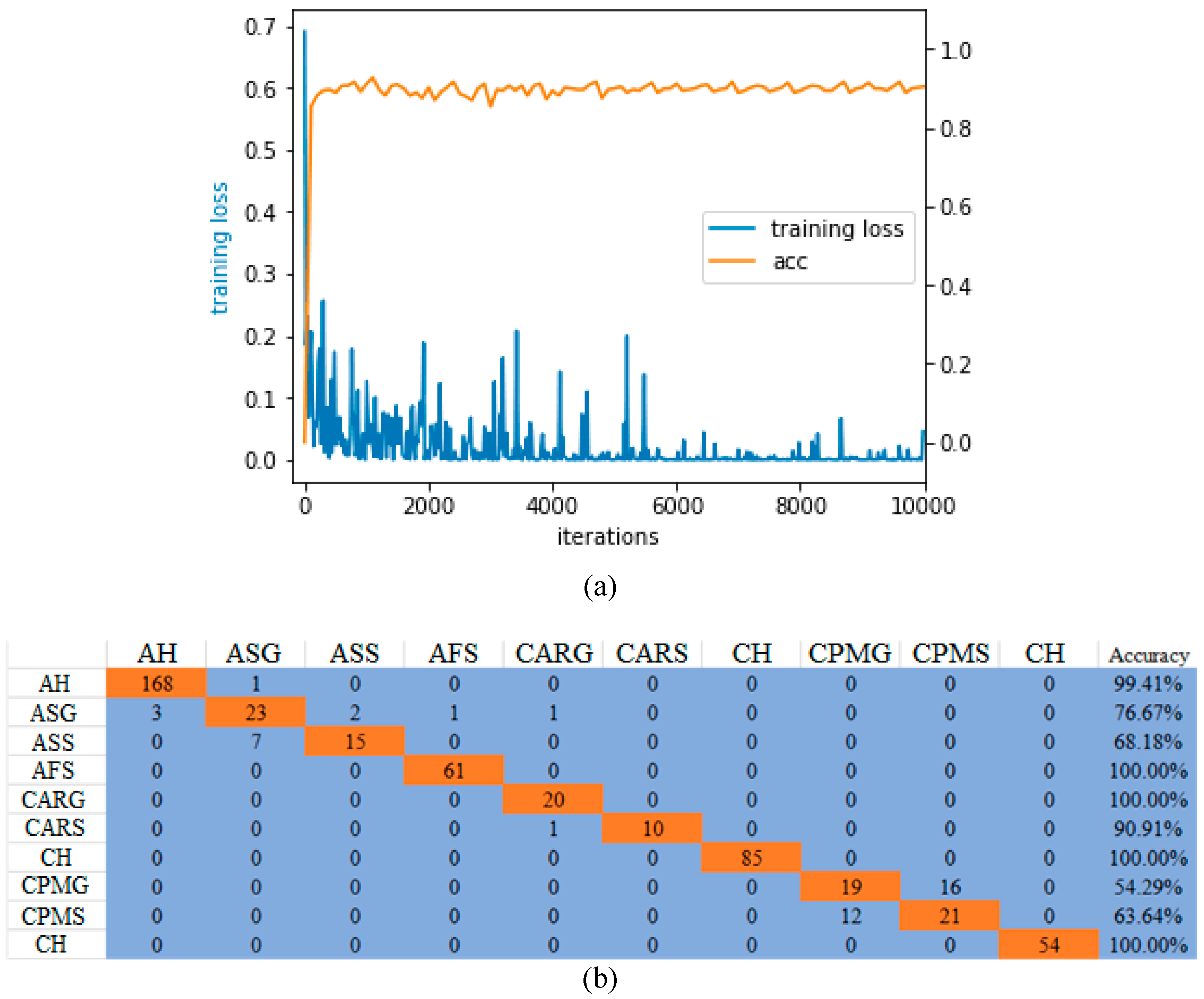
From Figure 8a, it can be concluded that our model tends to converge (blue curve), and the final accuracy rate is stable at 91.7% (orange curve), achieving a better classification result. Accuracy is an unreliable performance metric for evaluating the classification model because it can produce misleading results when the sample numbers of different classes in the data set are unevenly distributed. Moreover, the average accuracy of all categories is an accurate indicator for the model on the test set. In other words, the categories that are difficult to classify will be improved by the easily classified categories. The confusion matrix is the degree to which a classification model is accurate for each classification category. From the confusion matrix in Figure 9b, we can conclude that for some difficult-to-classify plant leaf diseases, the classification accuracy of such single-category on the test set is low, because the diseased region in each leaf is too small and the number of different grades of leaf disease is different. Therefore, it is difficult to be classified and identified by model. For instance, leaves of “Cherry Powdery Mildew – general” and those of “Cherry Powdery Mildew – serious” are difficult to be classified, because most of the regions in these leaves are very similar. The confusion matrix of the last experiment showed that the accuracy of disease recognition for corn is 100%, which did not interfere with other types of leaf diseases in classification.
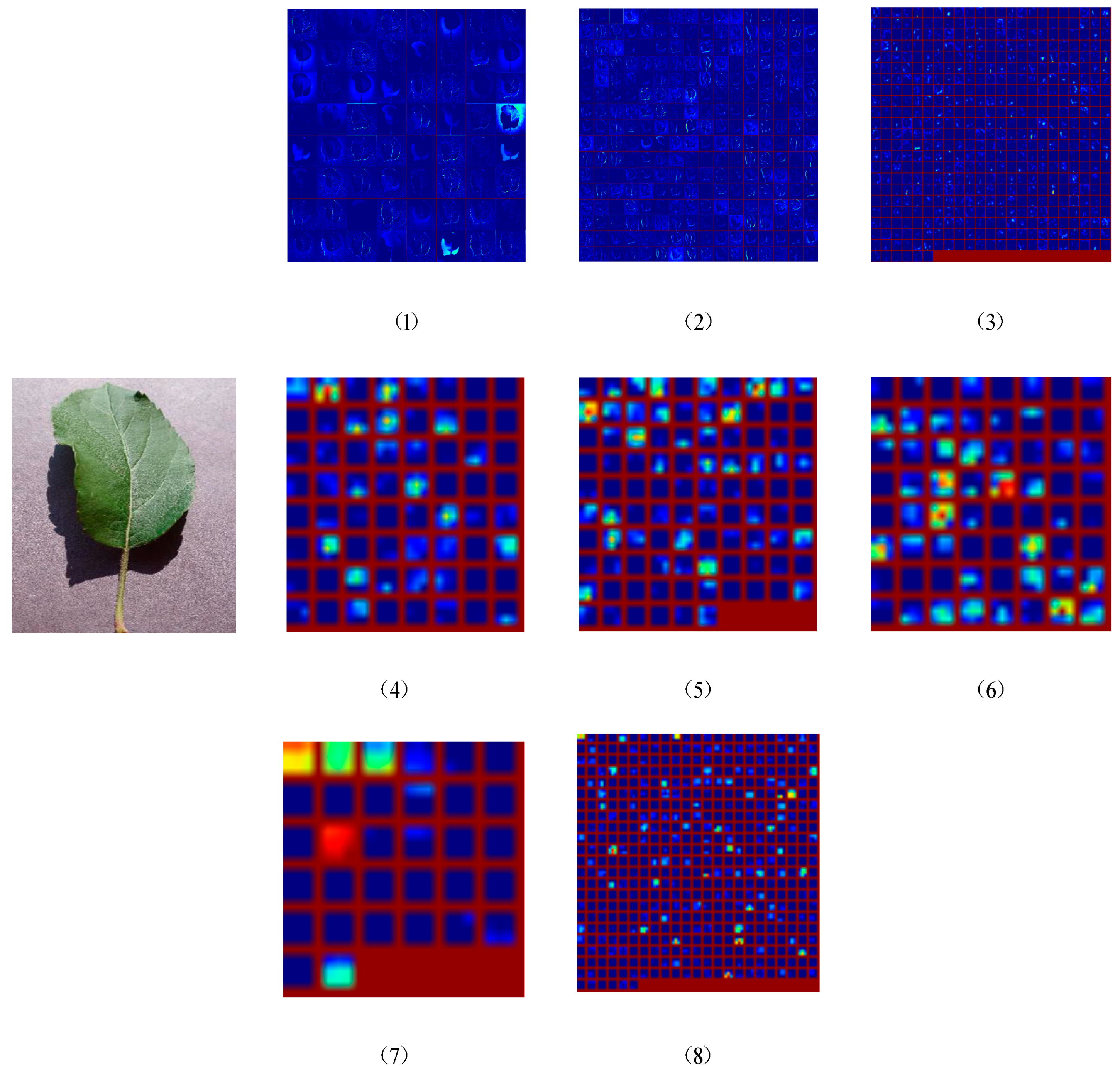
3.5. Visualization of Feature Extraction
Figure 9 visualizes a list of feature extractions after different layers of our network. The visualization of the network model can help us to intuitively understand the classification model. The ideal feature map of CNN should be sparse and contain typical local information. Through the visualization of the model, we can understand what features each layer of CNN learns, which can be used to adjust network parameters to improve the accuracy of the model. As a result, it provides a better understanding of how the CNN network learns the characteristics of the input image by visualizing various convolutional layers. We found that the features learned by CNN are hierarchical. The higher the level is, the more the specific features are presented. Moreover, the higher the dimensional feature maps correctly classify the images, the greater the effect presents. Specifically, the deep layer (Figure 9(7) or (8)) presents some edge corners and abstract features of colors, and the shallow feature map (Figure 9(1) or (2)) responds to the color information of the corners and other edges. The feature map of the middle layer (Figure 9(3), (4), (5), or (6)) has more complex invariance, captures similar textures, and has more layers for feature extraction. The high-level feature map shows the salient pose of the entire image after the extraction of the high-level abstract features.
4. Conclusions
This paper proposed an improved structure of convolutional neural networks for the identification and classification of a large dataset of different plant leaf diseases. Based on the traditional five-layer convolutional model of VGG16, the final, fully connected layer of VGG16 was replaced with Inception and SE modules, which can improve the classification accuracy of the model on the plant leaf disease dataset. Moreover, the global pooling layer can shorten the training time and parameter memory requirements, and also improve the generalization ability of the model. As a result, our method achieved the highest classification accuracy of 91.7% on the test set of plant leaf diseases. Compared with some other CNN methods, it has better adaptability to the change of image spatial position, showing better robustness to identify different diseases of various plant leaves, not limited to different diseases of the same plant.
Author Contributions
Conceptualization, P.C.; Data curation, J.H. and D.Z.; Funding acquisition, P.C.; Investigation, B.W.; Methodology, J.Z.; Project administration, P.C.; Software, J.Z. and D.Z.; Supervision, P.C. and D.Z.; Validation, B.W.; Writing–original draft, J.H.; Writing–review and editing, D.Z., P.C., B.W. and J.Z.
Funding
This work was supported by the National Natural Science Foundation of China (Nos. 61672035, 61472282, and 61872004), Educational Commission of Anhui Province (No. KJ2019ZD05), Anhui Province Funds for Excellent Youth Scholars in Colleges (gxyqZD2016068), the fund of Co-Innovation Center for Information Supply and Assurance Technology in AHU (ADXXBZ201705), and Anhui Scientific Research Foundation for Returness.
Conflicts of Interest
The authors declare no conflict of interest.
References
- Es-Saady, Y.; Massi, I.E.; Yassa, M.E.; Mammass, D.; Benazoun, A. Automatic Recognition of Plant Leaves Diseases Based on Serial Combination of Two SVM Classifiers. In Proceedings of the 2nd International Conference on Electrical and Information Technologies, Xi’an, China, 2–4 December 2016; pp. 561–566. [Google Scholar]
- Gavhale, M.K.R.; Gawande, U. An Overview of the Research on Plant Leaves Disease Detection Using Image Processing Techniques. IOSR J. Comput. Eng. 2014, 16, 10–16. [Google Scholar] [CrossRef]
- Wang, G.; Sun, Y.; Wang, J.X. Automatic Image Based Plant Disease Severity Estimation Using Deep Learning. Comput. Intell. Neurosci. 2017, 1–8. [Google Scholar] [CrossRef] [PubMed]
- Tan, F.; Ma, X.D. The Method of Recognition of Damage by Disease and Insect Based on Laminae. J. Agric. Mech. Res. 2009, 6, 41–43. [Google Scholar]
- Tian, Y.W.; Li, T.L.; Li, C.H. Method for Recognition of Grape Disease Based on Support Vector Machine. Trans. Chin. Soc. Agric. Eng. 2007, 23, 175–180. [Google Scholar]
- Wang, X.F.; Zhang, S.W.; Wang, Z. Recognition of Cucumber Diseases Based on Leaf Image and Environmental Information. Trans. Chin. Soc. Agric. Eng. 2014, 30, 148–153. [Google Scholar]
- Zhang, S.W.; Shang, Y.J.; Wang, L. Plant Disease Recognition Based on Plant Leaf Image. J. Anim. Plant Sci. 2015, 25, 42–45. [Google Scholar]
- Ron, B.; Yael, E. Human-robot collaborative site-specific sprayer. J. Field Robot. 2017, 34, 1519–1530. [Google Scholar]
- David, R.; Javier, M.M.; Emir, M. 3D Imaging with a Sonar Sensor and an Automated 3-Axes Frame for Selective Spraying in Controlled Conditions. J. Imaging 2017, 3, 9. [Google Scholar] [Green Version]
- Xie, C.; Wang, R.; Zhang, J.; Chen, P.; Dong, W.; Li, R.; Chen, T.; Chen, H. Multi-level learning features for automatic classification of field crop insects. Comput. Electron. Agric. 2018, 152, 233–241. [Google Scholar] [CrossRef]
- Sindhuja, S.; Ashish, M.; Reza, E. A review of advanced techniques for detecting plant diseases. Comput. Electron. Agric. 2010, 72, 1–13. [Google Scholar]
- Li, W.; Chen, P.; Wang, B.; Xie, C. Automatic Localization and Count of Agricultural Crop Pests Based on an Improved Deep Learning Pipeline. Sci. Rep. 2019, 9, 7024. [Google Scholar] [CrossRef] [PubMed]
- Yang, L.; Shu, J.Y.; Nian, Y.Z.; Yu, R.L.; Yong, Z. Identification of Rice Diseases Using Deep Convolutional Neural Networks. Neurocomputing 2017, 267, 378–384. [Google Scholar]
- Xia, D.; Chen, P.; Wang, B.; Zhang, J.; Xie, C. Insect detection and classification based on improved convolutional neural network. Sensors 2018, 18, 4169. [Google Scholar] [CrossRef] [PubMed]
- Sun, J.; Tan, W.J.; Mao, H.P.; Wu, X.H.; Chen, Y.; Wang, L. Identification of Leaf Diseases of Various Plants Based on Improved Convolutional Neural Network. Agric. Eng. Newsp. 2017, 19, 209–215. [Google Scholar]
- Mark, E.; Luc, V.G.; Christopher, K.I.; Williams, J.; Winn, A.Z. The Pascal Visual Object Classes (VOC) Challenge. Int. J. Comput. Vis. 2010, 88, 303–338. [Google Scholar]
- Deng, J.; Dong, W.; Socher, R.; Li, L.J.; Li, K.; Fei-Fei, L. Imagenet: A Large Scale Hierarchical Image Database. In Proceedings of the 2009 IEEE Conference on Computer Vision and Pattern Recognition, Miami, FL, USA, 20–25 June 2009; pp. 248–255. [Google Scholar]
- Russakovsky, O.; Deng, J.; Su, H.; Krause, J.; Satheesh, S.; Ma, S.; Huang, Z.; Karpathy, A.; Khosla, A.; Bernstein, M.; et al. ImageNet Large Scale Visual Recognition Challenge. Int. J. Comput. Vis. 2012, 115, 211–252. [Google Scholar] [CrossRef]
- Krizhevsky, A.; Sutskever, I.; Hinton, G.E. Imagenet Classification with Deep Convolutional Neural Networks. Available online: http://papers.nips.cc/paper/4824-imagenet-classification-with-deep-convolutional-neural-networks.pdf (accessed on 25 September 2019).
- Simonyan, K.; Zisserman, A.; Bengio, Y.; LeCun, Y. (Eds.) Very Deep Convolutional Networks for Large-Scale Image Recognition. In Proceedings of the 3rd International Conference on Learning Representations, San Diego, CA, USA, 7–9 May 2015. [Google Scholar]
- Szegedy, C.; Liu, W.; Jia, Y.; Sermanet, P.; Reed, S.E.; Anguelov, D.; Erhan, D.; Vanhoucke, V.; Rabinovich, A. Going Deeper with Convolutions. In Proceedings of the 28th IEEE Conference on Computer Vision and Pattern Recognition, Boston, MA, USA, 7–12 June 2015. [Google Scholar]
- He, K.; Zhang, X.; Ren, S.; Sun, J. Deep Residual Learning for Image Recognition. In Proceedings of the IEEE Conference on Computer Vision and Pattern Recognition, Boston, MA, USA, 7–12 June 2015; pp. 770–778. [Google Scholar]
- Hu, J.; Shen, L.; Sun, G. Squeeze-and-Excitation Networks. arXiv 2017, arXiv:1709.01507. [Google Scholar]
- Srivastava, N.; Hinton, G.E.; Krizhevsky, A.; Sutskever, I.; Salakhutdinov, R. Dropout: A simple way to prevent neural networks from overfitting. J. Mach. Learn. Res. 2014, 15, 1929–1958. [Google Scholar]
- Lin, M.; Chen, Q.; Yan, S. Network in network. arXiv 2013, arXiv:1312.4400. [Google Scholar]
- Jia, Y.; Shelhamer, E.; Donahue, J.; Karayev, S.; Long, J.; Girshick, R.; Guadarrama, S.; Darrell, T. Caffe: Convolutional Architecture for Fast Feature Embedding; Cornell University: Ithaca, NY, USA, 2014. [Google Scholar]
Figure 1.
Sample images of 10 leaf diseases. (1) Apple healthy (AH); (2) Apple Scab general (ASG); (3) Apple Scab serious (ASS); (4) Apple Frogeye Spot (AFS); (5) Cedar Apple Rust genera (CARG)l; (6) Cedar Apple Rust serious (CARS); (7) Cherry healthy (CH); (8) Cherry Powdery Mildew general (CPMG); (9) Cherry Powdery Mildew serious (CPMS); (10) Corn healthy (CH).

Figure 2.
The structure of the proposed convolutional neural network (CNN).

Figure 3.
Inception structure model.

Figure 4.
Comparison of the fully connected layer and the global averaged pooled layer.

Figure 5.
Squeeze-and-Excitation (SE) module.

Figure 6.
The combined structure of the SE module and the Inception structure.

Figure 7.
Trends in the accuracy of different CNN models on the test set.

Figure 8.
Trend graph of the loss function (a) and confusion matrix (b). (1) Apple healthy (AH); (2) Apple Scab general (ASG); (3) Apple Scab serious (ASS); (4) Apple Frogeye Spot (AFS); (5) Cedar Apple Rust genera (CARG)l; (6) Cedar Apple Rust serious (CARS); (7) Cherry healthy (CH); (8) Cherry Powdery Mildew general (CPMG); (9) Cherry Powdery Mildew serious (CPMS); (10) Corn healthy (CH).

Figure 9.
Visualization of feature map from each layer for a sample leaf. (1) conv1_1 (see Table 2), (2) conv3_1, (3) conv5_1, (4) inception_ 1 × 1, (5) inception_ 3 × 3, (6) inception_ 5 × 5, (7) inception_ pool, (8) pool7.
Figure 9.
Visualization of feature map from each layer for a sample leaf. (1) conv1_1 (see Table 2), (2) conv3_1, (3) conv5_1, (4) inception_ 1 × 1, (5) inception_ 3 × 3, (6) inception_ 5 × 5, (7) inception_ pool, (8) pool7.


Table 1.
Statistics of the plant leaf disease dataset.
| Class | Number of Training Images (Before Data Augmentation) | Number of Training Images (After Data Augmentation) | Number of Testing Images |
|---|---|---|---|
| Apple healthy | 1185 | 1185 | 169 |
| Apple Scab general | 844 | 844 | 30 |
| Apple Scab serious | 596 | 596 | 22 |
| Apple Frogeye Spot | 427 | 427 | 61 |
| Cedar Apple Rust general | 142 | 142 | 20 |
| Cedar Apple Rust serious | 40 | 160 | 11 |
| Cherry healthy | 598 | 598 | 85 |
| Cherry Powdery Mildew general | 162 | 648 | 35 |
| Cherry Powdery Mildew serious | 153 | 612 | 33 |
| Corn healthy | 376 | 376 | 54 |
| Total | 4523 | 5588 | 520 |
Table 2.
Related parameters of the convolutional neural network (CNN)-based model.
| Type | Size/Stride | Output Size |
|---|---|---|
| Conv1 (Convolutional layer 1) | 3 × 3/1 | 64 × 224 × 224 |
| Pool1/max | 3 × 3/1 | 64 × 112 × 112 |
| Conv2 | 3 × 3/1 | 128 × 112 × 112 |
| Pool2/max | 3 × 3/1 | 128 × 56 × 56 |
| Conv3 | 3 × 3/1 | 256 × 56 × 56 |
| Pool3/max | 3 × 3/1 | 256 × 28 × 28 |
| Conv4 | 3 × 3/1 | 512 × 28 × 28 |
| Pool4/max | 3 × 3/1 | 512 × 14 × 14 |
| Conv5 | 3 × 3/1 | 512 × 14 × 14 |
| Pool5/max | 3 × 3/1 | 512 × 7 × 7 |
| Pool6/max | 3 × 3/1 | 512 × 3 × 3 |
| Inception | - | 256 × 3 × 3 |
| Pool7/ave | 3 × 3/1 | 256 × 1 × 1 |
| Dropout | - | 256 × 1 × 1 |
| Linear | - | 10 × 1 × 1 |
| Softmax | - | 10 |
Table 3.
Classification accuracy (in percent) comparison of CNN-Based models.
| CNN | Accuracy | Model Size | Training Time |
|---|---|---|---|
| AlexNet | 0.894 | 217 MB | 1140.15 s |
| GoogLeNet | 0.898 | 47.1 MB | 332.228 s |
| VGG16 | 0.905 | 537.2 MB | 1960.2 s |
| VGG19 | 0.903 | 558.4 MB | 5411.31 s |
| ResNet-50 | 0.901 | 94.3 MB | 2101.19 s |
| Inceptionv2 | 0.903 | 45.1 MB | 2187.3 s |
| Inceptionv3 | 0.901 | 87.4 MB | 6438.72 s |
| Inceptionv4 | 0.89 | 165 MB | 5787.9 s |
| SENet | 0.875 | 220.8 MB | 1794.78 s |
| Our method | 0.917 | 57.3 MB | 961.1 s |
Table 4.
Comparison of training time for different CNN models.
| CNN | Forward Pass | Backward Pass | Total Time |
|---|---|---|---|
| AlexNet | 0.052 s | 0.061 s | 1140.15 s |
| GoogLeNet | 0.013 s | 0.019 s | 332.228 s |
| VGG16 | 0.047 s | 0.014 s | 1960.2 s |
| VGG19 | 0.167 s | 0.371 s | 5411.31 s |
| ResNet-50 | 0.096 s | 0.114 s | 2101.19 s |
| Inceptionv2 | 0.102 s | 0.117 s | 2187.3 s |
| Inceptionv3 | 0.301 s | 0.342 s | 6438.72 s |
| Inceptionv4 | 0.258 s | 0.321 s | 5787.9 s |
| SENet | 0.116 s | 0.179 s | 1794.78 s |
| Our method | 0.038 s | 0.053 s | 961.1 s |
© 2019 by the authors. Licensee MDPI, Basel, Switzerland. This article is an open access article distributed under the terms and conditions of the Creative Commons Attribution (CC BY) license (http://creativecommons.org/licenses/by/4.0/).
Share and Cite
MDPI and ACS Style
Hang, J.; Zhang, D.; Chen, P.; Zhang, J.; Wang, B. Classification of Plant Leaf Diseases Based on Improved Convolutional Neural Network. Sensors 2019, 19, 4161. https://doi.org/10.3390/s19194161
AMA Style
Hang J, Zhang D, Chen P, Zhang J, Wang B. Classification of Plant Leaf Diseases Based on Improved Convolutional Neural Network. Sensors. 2019; 19(19):4161. https://doi.org/10.3390/s19194161
Chicago/Turabian StyleHang, Jie, Dexiang Zhang, Peng Chen, Jun Zhang, and Bing Wang. 2019. "Classification of Plant Leaf Diseases Based on Improved Convolutional Neural Network" Sensors 19, no. 19: 4161. https://doi.org/10.3390/s19194161
Note that from the first issue of 2016, this journal uses article numbers instead of page numbers. See further details here.