Spatial and Temporal Distribution of PM2.5 Pollution over Northeastern Mexico: Application of MERRA-2 Reanalysis Datasets

 , ,
, , 

Abstract
:1. Introduction
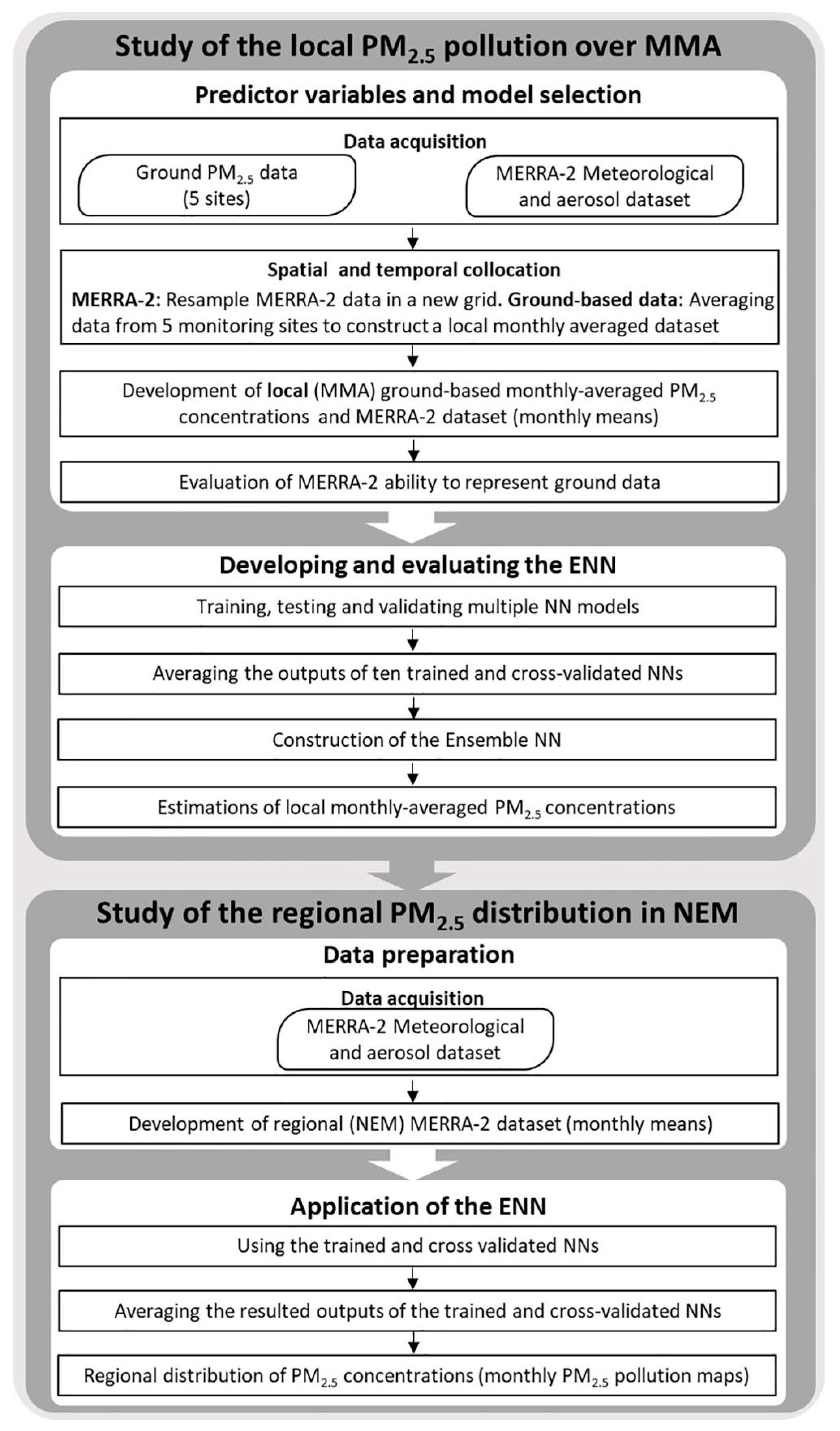
2. Data and Methods
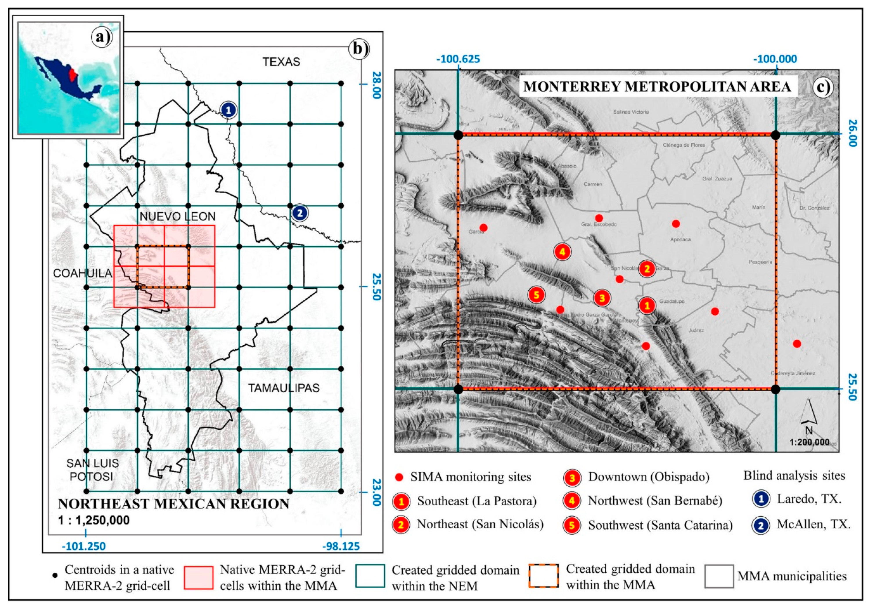
2.1. Study Area
2.2. Ground-Based PM2.5 and Meteorological Data
2.3. PM2.5 and Meteorological Data from MERRA-2
2.4. Spatial and Temporal Collocation
2.5. Evaluation of MERRA-2’s Ability to Represent Ground Data and Model Selection
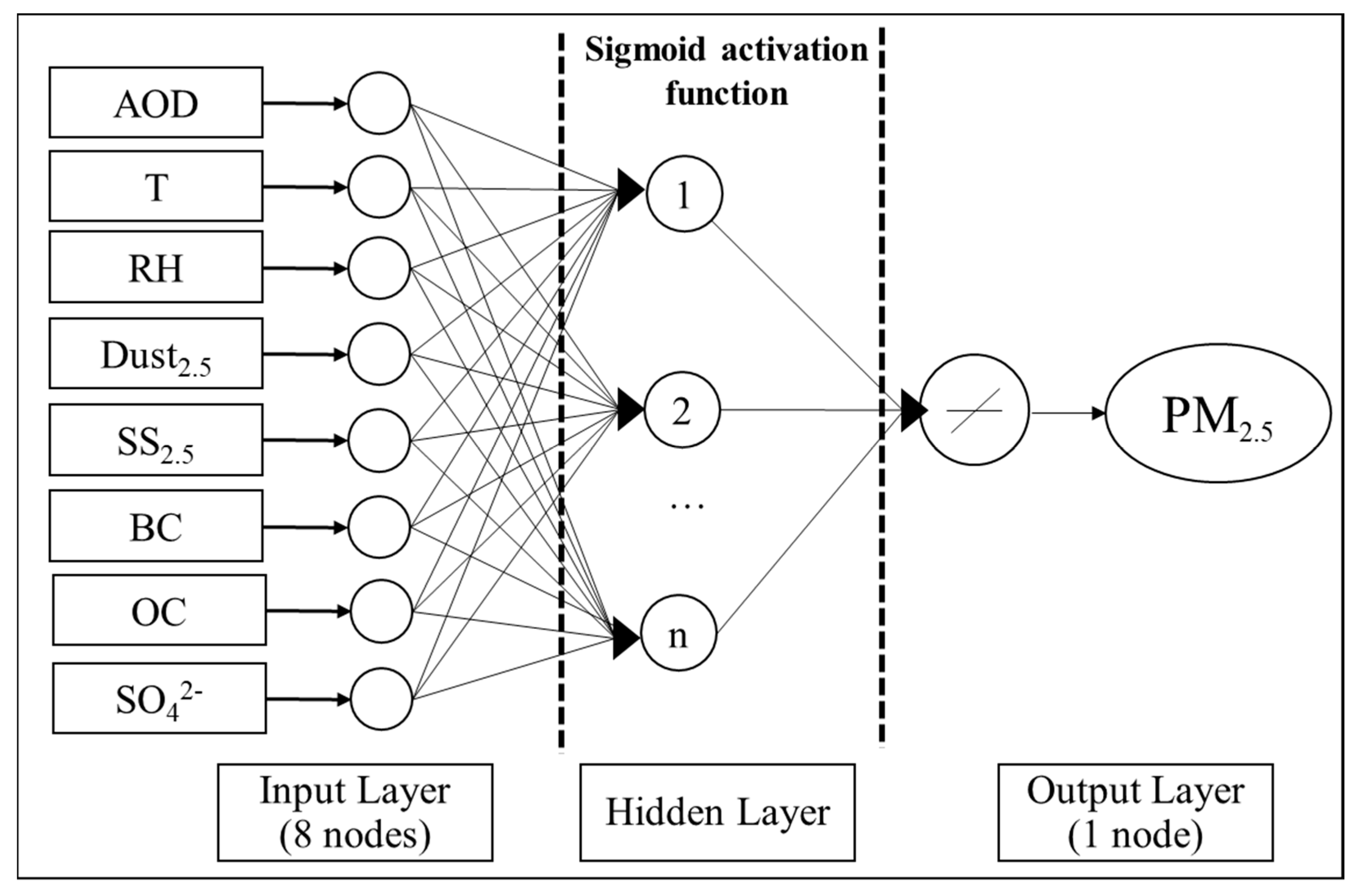
2.6. Model Development
3. Results
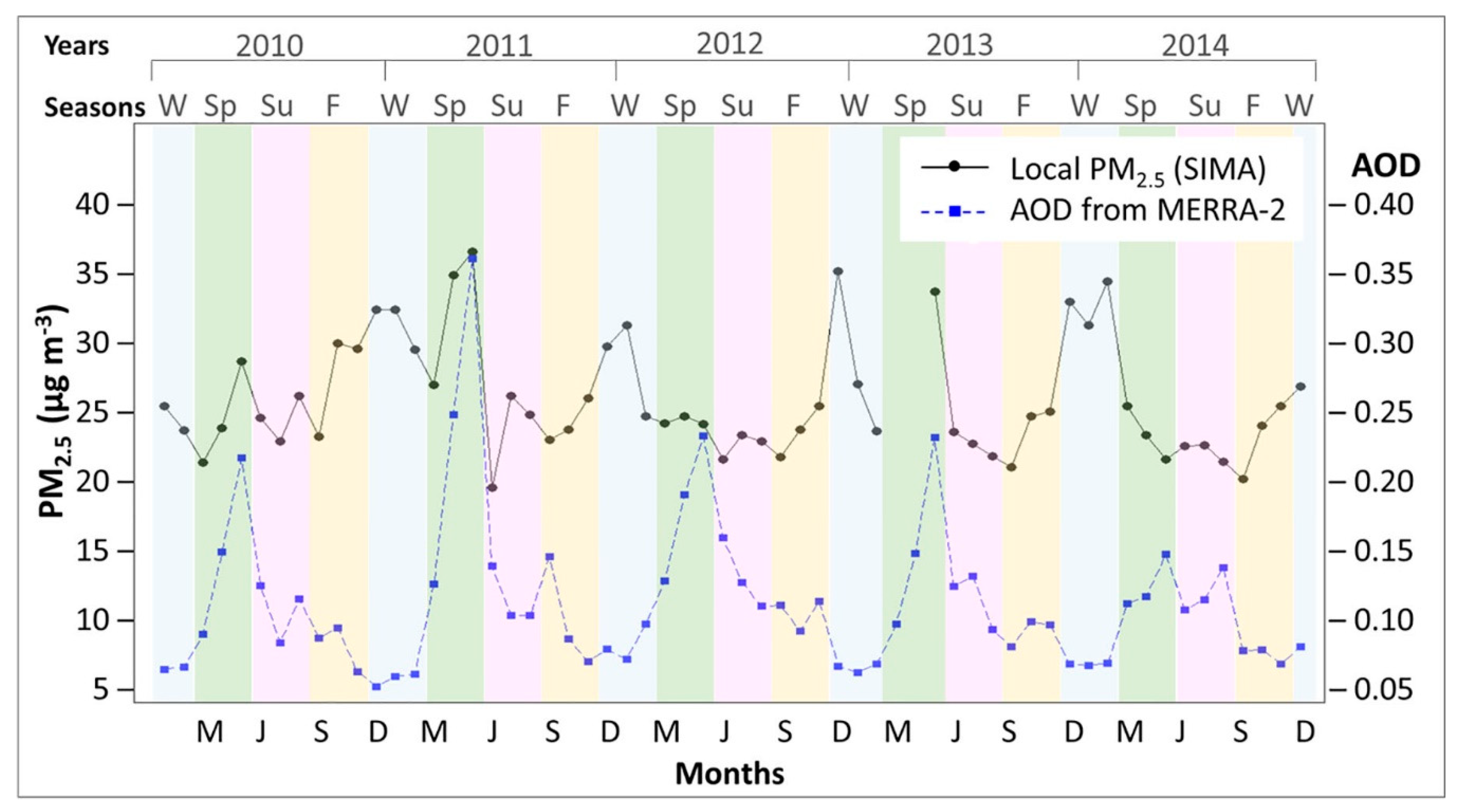
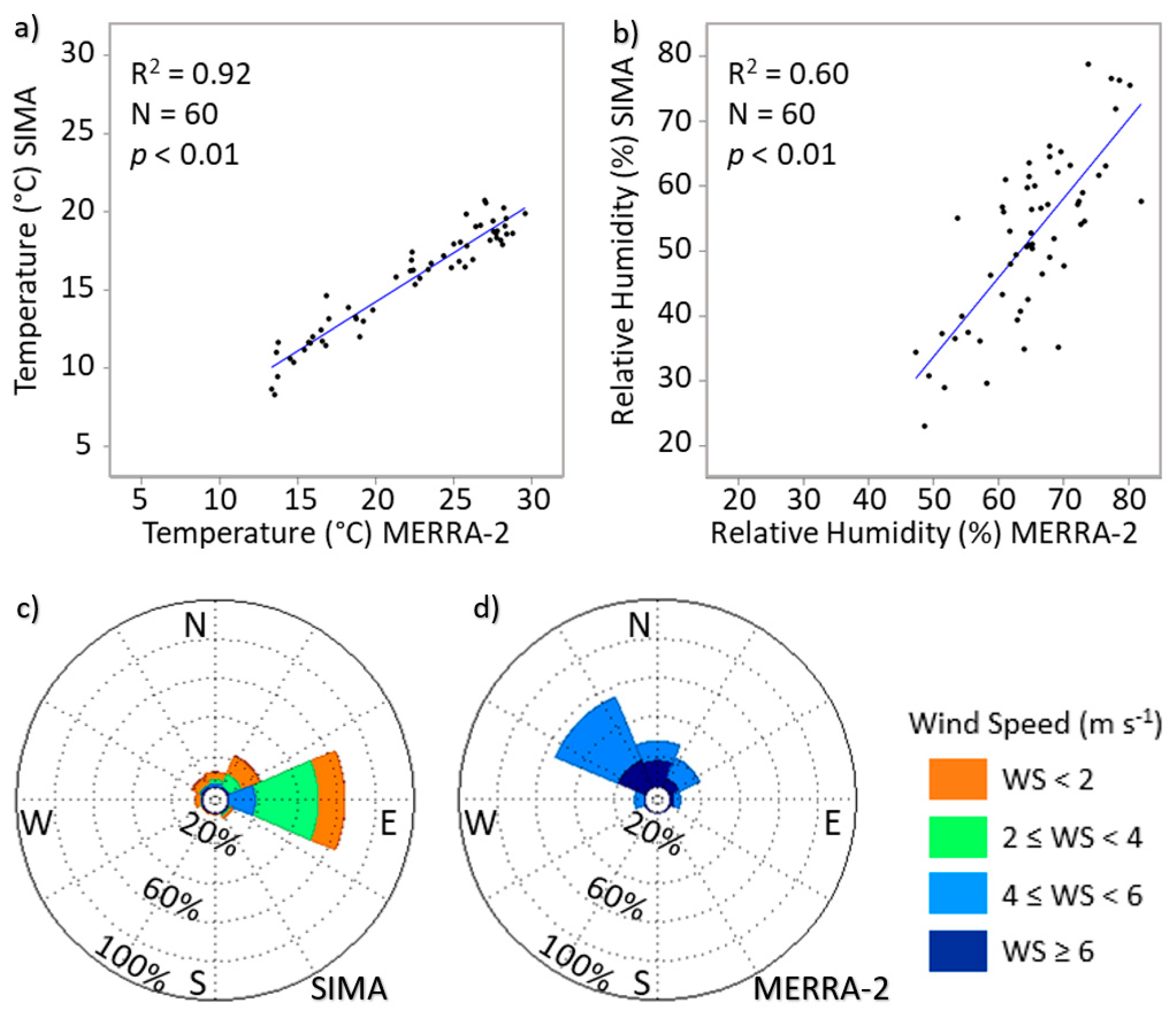
3.1. MERRA-2 and Ground-Based Data: Comparisons
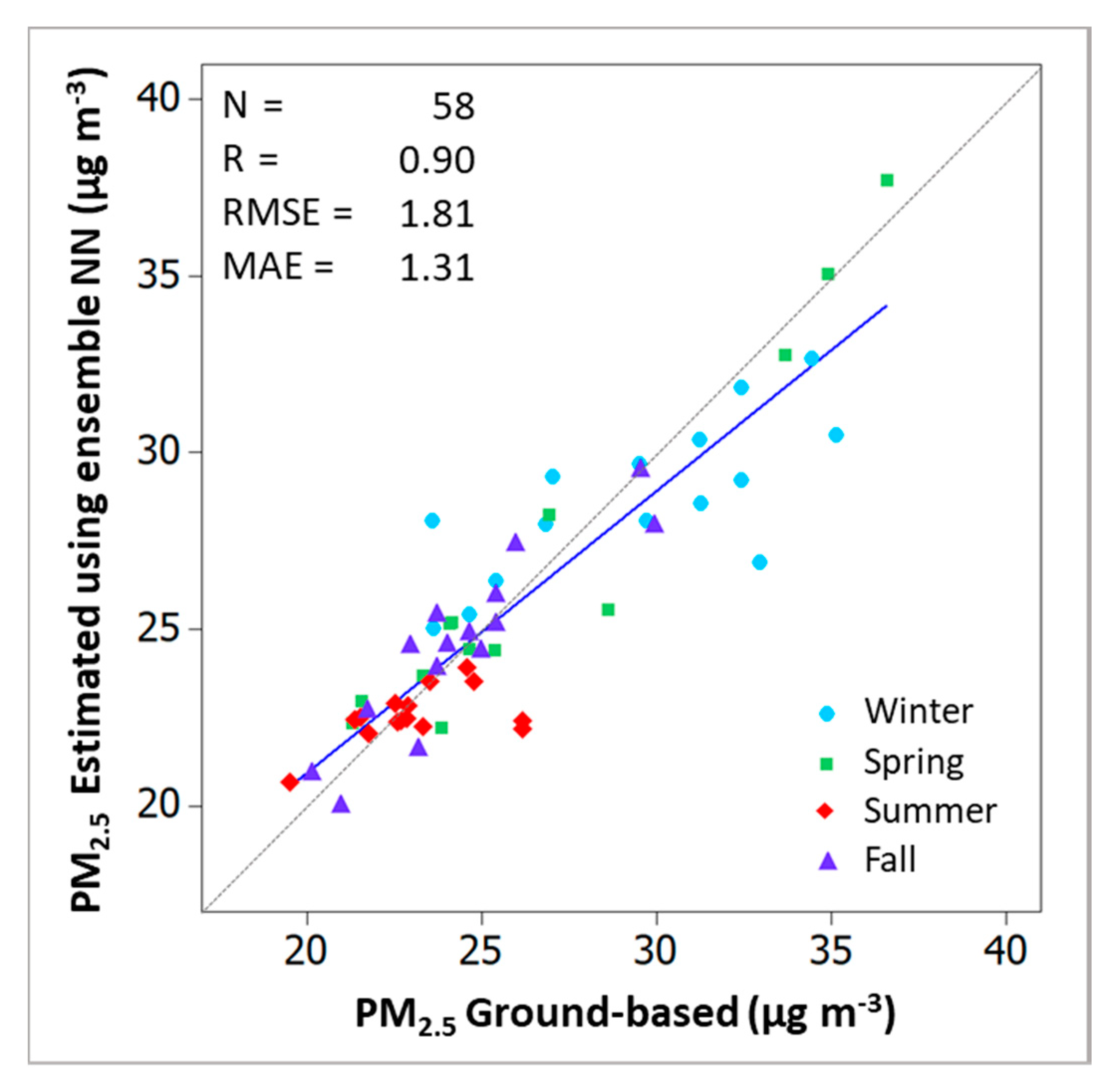
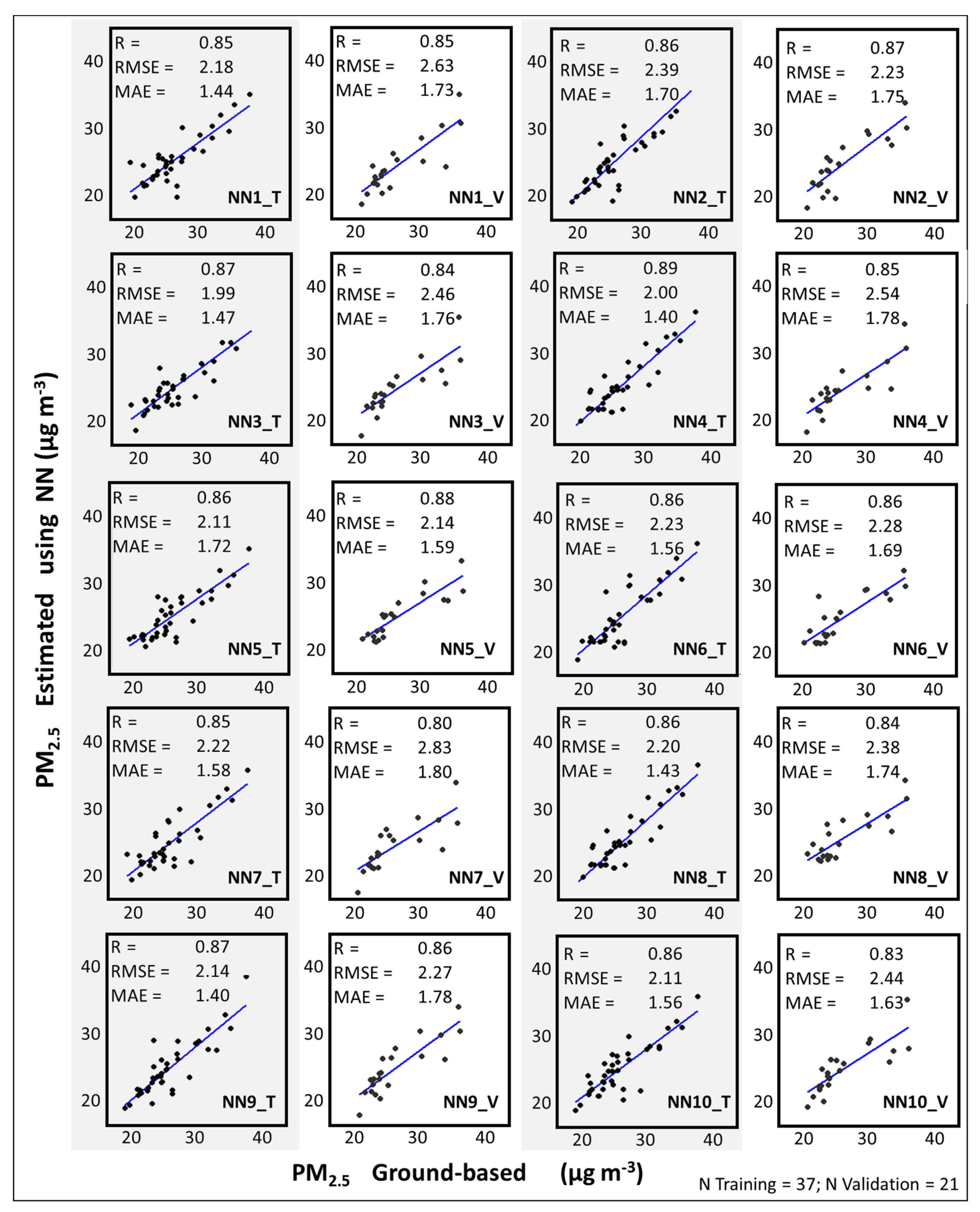
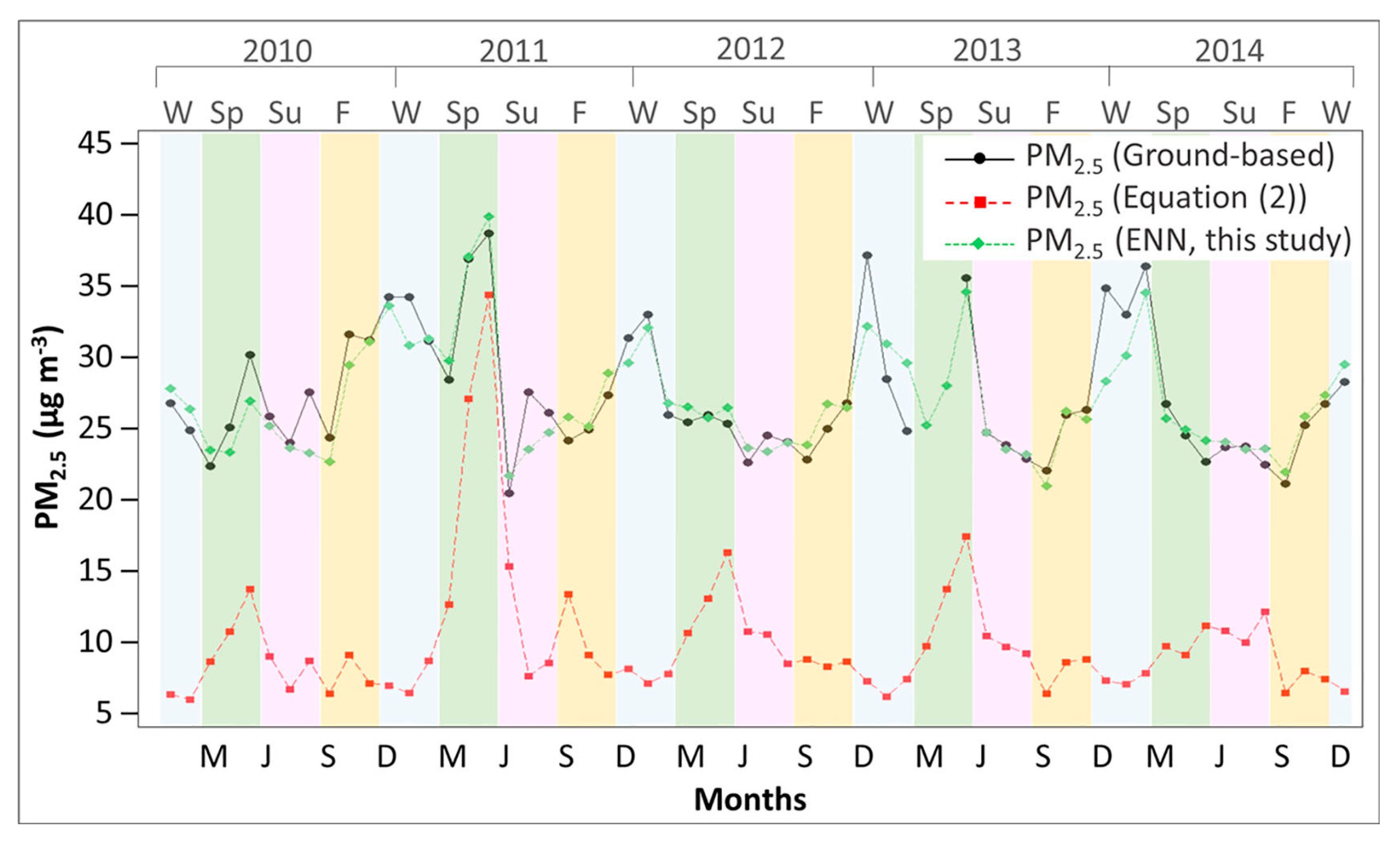
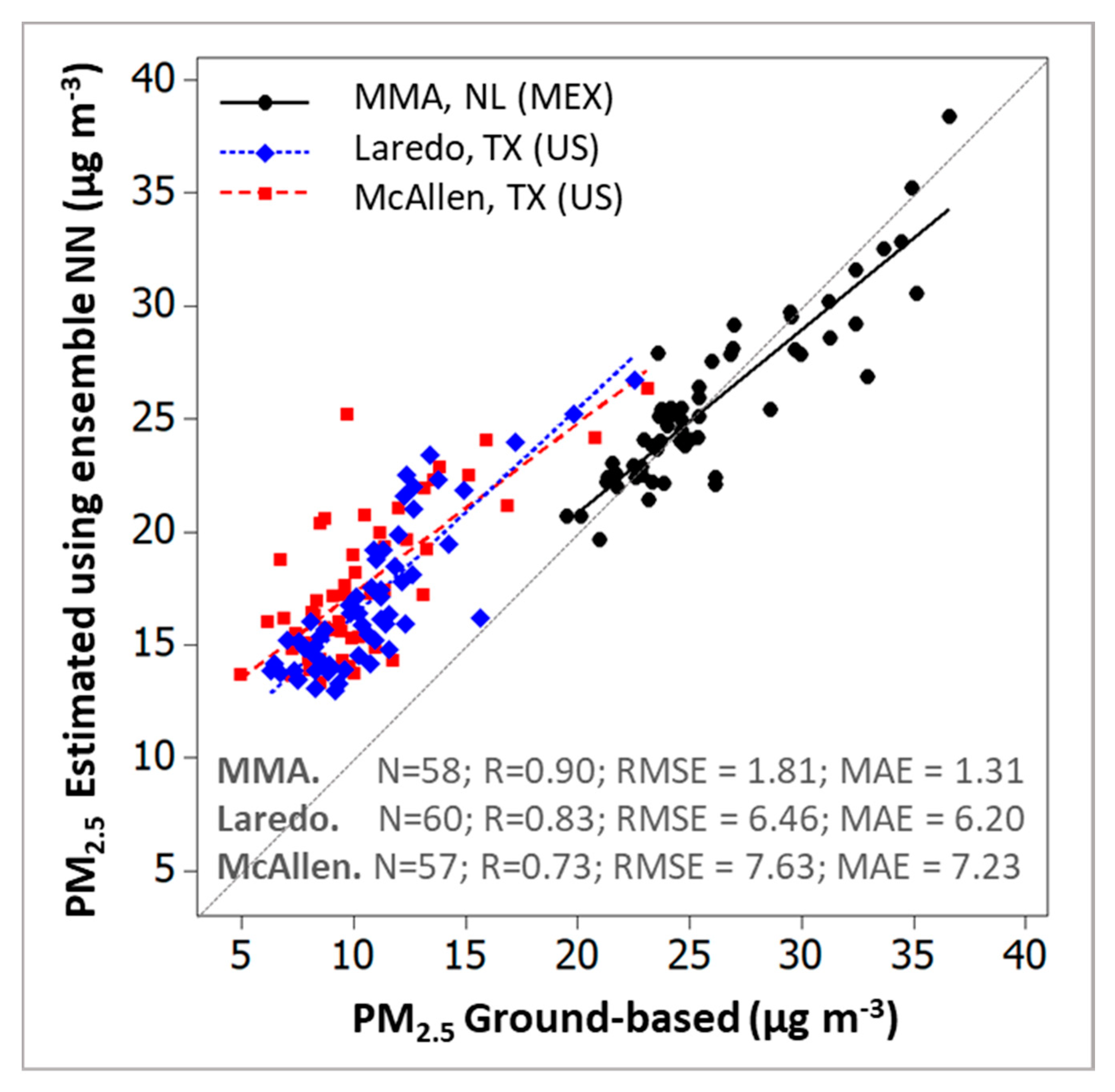
3.2. Model Performance
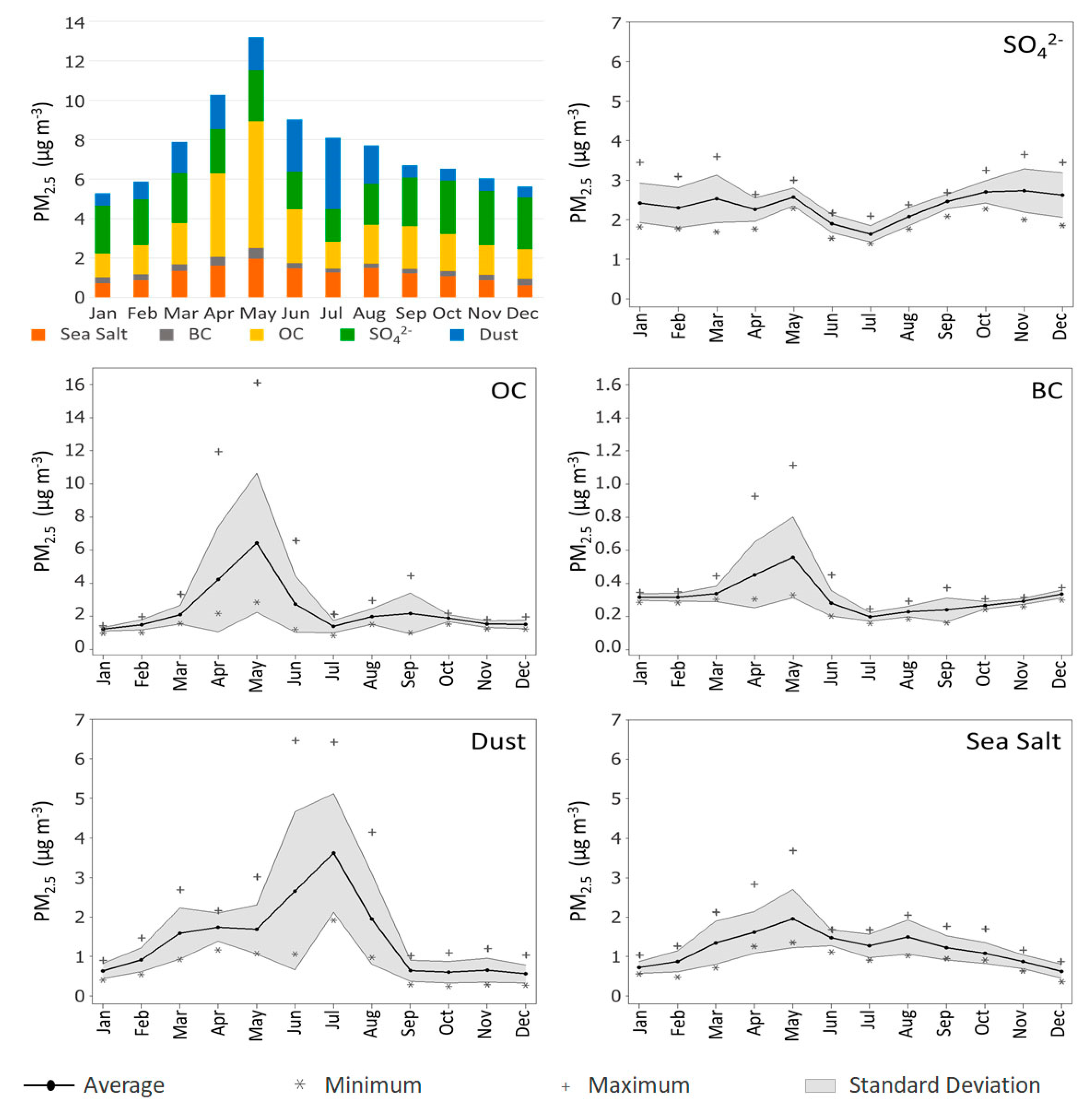
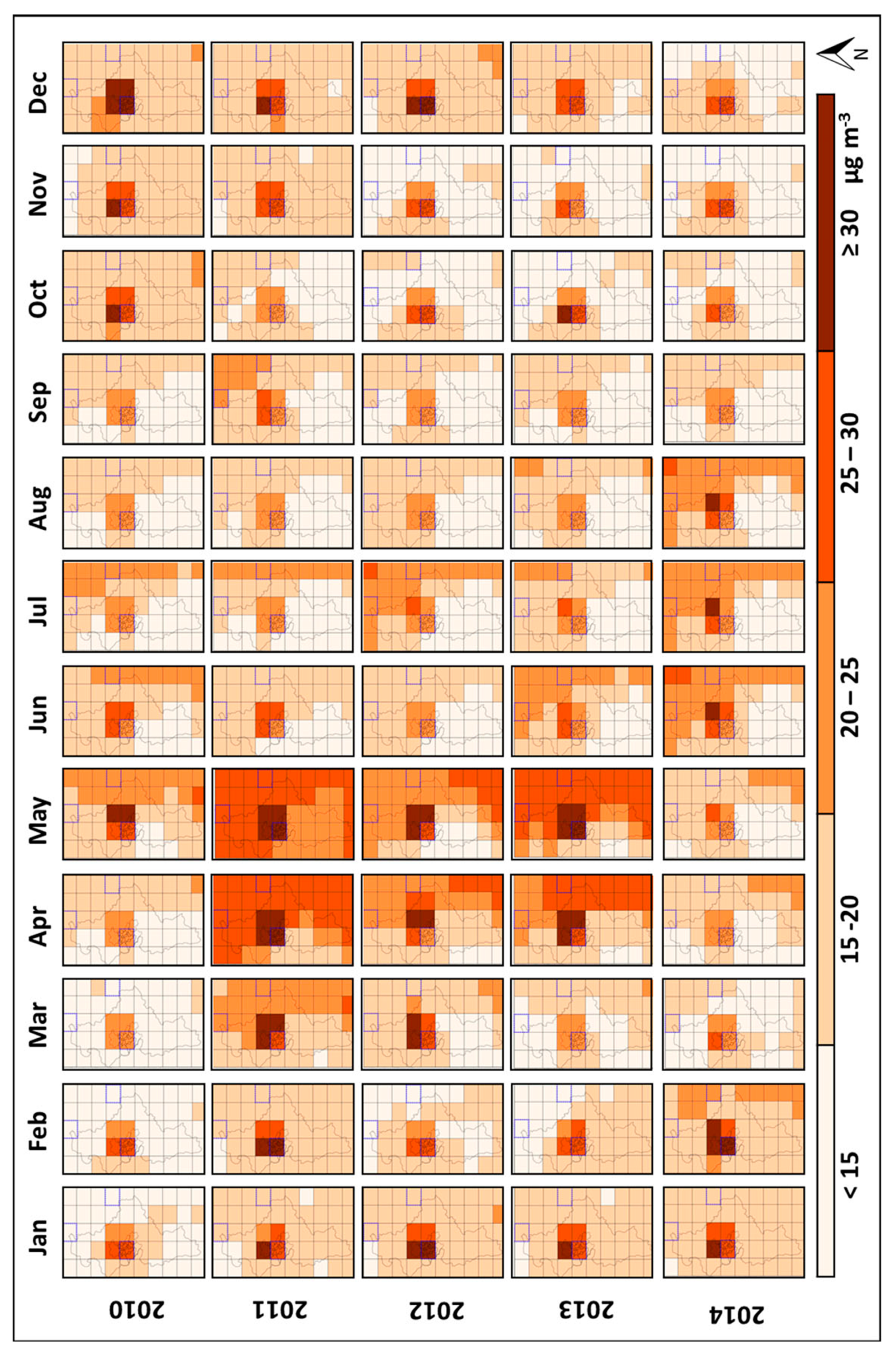
3.3. Regional PM2.5 Distribution
4. Discussion
5. Conclusions
Author Contributions
Acknowledgments
Conflicts of Interest
References
- Cheng, Z.; Luo, L.; Wang, S.; Wang, Y.; Sharma, S.; Shimadera, H.; Wang, X.; Bressi, M.; Miranda, R.; Jiang, J.; et al. Status and characteristics of ambient PM2.5 pollution in global megacities. Environ. Int. 2016, 89–90. [Google Scholar] [CrossRef] [PubMed]
- Fu, P.; Guo, X.; Cheung, F.M.H.; Yung, K.K.L. The association between PM2.5 exposure and neurological disorders: A systematic review and meta-analysis. Sci. Total Environ. 2019, 655, 1240–1248. [Google Scholar] [CrossRef]
- Gutiérrez-Avila, I.; Rojas-Bracho, L.; Riojas-Rodríguez, H.; Kloog, I.; Just, A.C.; Rothenberg, S.J. Cardiovascular and cerebrovascular mortality associated with acute exposure to PM2.5 in Mexico City. Stroke 2018, 49, 1734–1736. [Google Scholar] [CrossRef] [PubMed]
- Fajersztajn, L.; Saldiva, P.; Pereira, L.A.A.; Leite, V.F.; Buehler, A.M. Short-term effects of fine particulate matter pollution on daily health events in Latin America: A systematic review and meta-analysis. Int. J. Public Health 2017, 62, 729–738. [Google Scholar] [CrossRef] [PubMed]
- Yang, S.; Lee, S.-P.; Park, J.-B.; Lee, H.; Kang, S.-H.; Lee, S.-E.; Kim, J.B.; Choi, S.-Y.; Kim, Y.-J.; Chang, H.-J. PM2.5 concentration in the ambient air is a risk factor for the development of high-risk coronary plaques. Eur. Heart J. Cardiovasc. Imaging 2019, 20, 1355–1364. [Google Scholar] [CrossRef] [Green Version]
- Gao, M.; Cao, J.; Seto, E. A distributed network of low-cost continuous reading sensors to measure spatiotemporal variations of PM2.5 in Xi’an, China. Environ. Pollut. 2015, 199, 56–65. [Google Scholar] [CrossRef] [PubMed] [Green Version]
- Song, Z.; Fu, D.; Zhang, X.; Wu, Y.; Xia, X.; He, J. Diurnal and seasonal variability of PM2.5 and AOD in North China plain: Comparison of MERRA-2 products and ground measurements. Atmos. Environ. 2018, 191, 70–78. [Google Scholar] [CrossRef]
- Idrees, Z.; Zheng, L. Low cost air pollution monitoring systems: A review of protocols and enabling technologies. J. Ind. Inf. Integr. 2020, 17, 100123. [Google Scholar] [CrossRef]
- Riojas-Rodriguez, H.; Soares da Silva, A.; Texcalac Sangrador, J.L.; Moreno-Banda, G. Air pollution management and control in Latin America and the Caribbean: Implications for climate change. Rev. Panam. De Salud Pública 2016, 40, 150–159. [Google Scholar]
- PurpleAir. PurpleAir Map. Available online: https://www.purpleair.com/map?opt=1/mAQI/a10/cC0#11/25.6414/-100.2937 (accessed on 16 March 2020).
- Gupta, P.; Doraiswamy, P.; Levy, R.; Pikelnaya, O.; Maibach, J.; Feenstra, B.; Polidori, A.; Kiros, F.; Mills, K.C. Impact of California fires on local and regional air quality: The role of a low-cost sensor network and satellite observations. GeoHealth 2018, 2, 172–181. [Google Scholar] [CrossRef]
- Rogulski, M. Using low-cost PM monitors to detect local changes of air quality. Pol. J. Environ. Stud. 2018, 27. [Google Scholar] [CrossRef]
- Chu, D.A.; Kaufman, Y.J.; Zibordi, G.; Chern, J.D.; Mao, J.; Li, C.; Holben, B.N. Global monitoring of air pollution over land from the earth observing system-terra moderate resolution imaging spectroradiometer (MODIS). J. Geophys. Res. D Atmos. 2003, 108, 1–18. [Google Scholar] [CrossRef]
- van Donkelaar, A.; Martin, R.V.; Park, R.J. Estimating ground-level PM2.5 using aerosol optical depth determined from satellite remote sensing. J. Geophys. Res. Atmos. 2006, 111, 1–10. [Google Scholar] [CrossRef]
- Levy, R.C.; Mattoo, S.; Munchak, L.A.; Remer, L.A.; Sayer, A.M.; Patadia, F.; Hsu, N.C. The collection 6 MODIS aerosol products over land and ocean. Atmos. Meas. Tech. 2013, 6, 2989–3034. [Google Scholar] [CrossRef] [Green Version]
- Shin, S.-K.; Tesche, M.; Müller, D.; Noh, Y. Technical note: Absorption aerosol optical depth components from AERONET observations of mixed dust plumes. Atmos. Meas. Tech. 2019, 12, 607–618. [Google Scholar] [CrossRef] [Green Version]
- Randles, C.A.; da Silva, A.M.; Buchard, V.; Colarco, P.R.; Darmenov, A.; Govindaraju, R.; Smirnov, A.; Holben, B.; Ferrare, R.; Hair, J.; et al. The MERRA-2 aerosol reanalysis, 1980 onward. Part I: System description and data assimilation evaluation. J. Clim. 2017, 30, 6823–6850. [Google Scholar] [CrossRef]
- Provençal, S.; Kishcha, P.; da Silva, A.M.; Elhacham, E.; Alpert, P. AOD distributions and trends of major aerosol species over a selection of the world’s most populated cities based on the 1st version of NASA’s MERRA aerosol reanalysis. Urban Clim. 2017, 20, 168–191. [Google Scholar] [CrossRef]
- Qin, W.; Zhang, Y.; Chen, J.; Yu, Q.; Cheng, S.; Li, W.; Liu, X.; Tian, H. Variation, sources and historical trend of black carbon in Beijing, China based on ground observation and MERRA-2 reanalysis data. Environ. Pollut. 2019, 245, 853–863. [Google Scholar] [CrossRef]
- Xu, X.; Yang, X.; Zhu, B.; Tang, Z.; Wu, H.; Xie, L. Characteristics of MERRA-2 black carbon variation in east China during 2000–2016. Atmos. Environ. 2020, 222, 117140. [Google Scholar] [CrossRef]
- Sitnov, S.A.; Mokhov, I.I.; Likhosherstova, A.A. Exploring large-scale black-carbon air pollution over Northern Eurasia in summer 2016 using MERRA-2 reanalysis data. Atmos. Res. 2020, 235, 104763. [Google Scholar] [CrossRef]
- Mukkavilli, S.K.; Prasad, A.A.; Taylor, R.A.; Huang, J.; Mitchell, R.M.; Troccoli, A.; Kay, M.J. Assessment of atmospheric aerosols from two reanalysis products over Australia. Atmos. Res. 2019, 215, 149–164. [Google Scholar] [CrossRef] [Green Version]
- García-Franco, J.L. Air quality in Mexico City during the fuel shortage of January 2019. Atmos. Environ. 2020, 222. [Google Scholar] [CrossRef]
- Gardner, M.W.; Dorling, S.R. Artificial neural networks (the multilayer perceptron)—A review of applications in the atmospheric sciences. Atmos. Environ. 1998, 32, 2627–2636. [Google Scholar] [CrossRef]
- Karimian, H.; Li, Q.; Wu, C.; Qi, Y.; Mo, Y.; Chen, G.; Zhang, X.; Sachdeva, S. Evaluation of different machine learning approaches to forecasting PM2.5 mass concentrations. Aerosol Air Qual. Res. 2019, 19, 1400–1410. [Google Scholar] [CrossRef] [Green Version]
- Sadorsky, P. Modeling and forecasting petroleum futures volatility. Energy Econ. 2006, 28, 467–488. [Google Scholar] [CrossRef]
- Bai, Y.; Li, Y.; Wang, X.; Xie, J.; Li, C. Air pollutants concentrations forecasting using back propagation neural network based on wavelet decomposition with meteorological conditions. Atmos. Pollut. Res. 2016, 7, 557–566. [Google Scholar] [CrossRef]
- Chen, L.; Pai, T.Y. Comparisons of GM (1,1), and BPNN for predicting hourly particulate matter in Dali area of Taichung city, Taiwan. Atmos. Pollut. Res. 2015, 6, 572–580. [Google Scholar] [CrossRef] [Green Version]
- Durão, R.M.; Mendes, M.T.; João Pereira, M. Forecasting O3 levels in industrial area surroundings up to 24 h in advance, combining classification trees and MLP models. Atmos. Pollut. Res. 2016, 7, 961–970. [Google Scholar] [CrossRef] [Green Version]
- Wang, D.; Wei-Zhen, L. Forecasting of ozone level in time series using MLP model with a novel hybrid training algorithm. Atmos. Environ. 2006, 40, 913–924. [Google Scholar] [CrossRef]
- Iliyas, S.A.; Elshafei, M.; Habib, M.A.; Adeniran, A.A. RBF neural network inferential sensor for process emission monitoring. Control Eng. Pract. 2013, 21, 962–970. [Google Scholar] [CrossRef]
- Lu, W.Z.; Wang, W.J.; Wang, X.K.; Yan, S.H.; Lam, J.C. Potential assessment of a neural network model with PCA/RBF approach for forecasting pollutant trends in Mong Kok urban air, Hong Kong. Environ. Res. 2004, 96, 79–87. [Google Scholar] [CrossRef] [PubMed]
- Maleki, H.; Sorooshian, A.; Goudarzi, G.; Baboli, Z.; Tahmasebi Birgani, Y.; Rahmati, M. Air pollution prediction by using an artificial neural network model. Clean Technol. Environ. Policy 2019, 21, 1341–1352. [Google Scholar] [CrossRef]
- Prasad, K.; Gorai, A.K.; Goyal, P. Development of ANFIS models for air quality forecasting and input optimization for reducing the computational cost and time. Atmos. Environ. 2016, 128, 246–262. [Google Scholar] [CrossRef]
- Taheri Shahraiyni, H.; Sodoudi, S.; Kerschbaumer, A.; Cubasch, U. A new structure identification scheme for ANFIS and its application for the simulation of virtual air pollution monitoring stations in urban areas. Eng. Appl. Artif. Intell. 2015, 41, 175–182. [Google Scholar] [CrossRef] [Green Version]
- Cabaneros, S.M.; Calautit, J.K.; Hughes, B.R. A review of artificial neural network models for ambient air pollution prediction. Environ. Model. Softw. 2019, 119, 285–304. [Google Scholar] [CrossRef]
- Liu, Y. New directions: Satellite driven PM2.5 exposure models to support targeted particle pollution health effects research. Atmos. Environ. 2013, 68, 52–53. [Google Scholar] [CrossRef]
- Secretaría de Desarrollo Agrario, Territorial y Urbano, Consejo Nacional de Población and Instituto Nacional de Estadística y Geografía. In Delimitación de las Zonas Metropolitanas de México 2015; Secretaría de Gobernación: Mexico City, Mexico, 2018.
- González-Santiago, O.; Badillo-Castañeda, C.T.; Kahl, J.D.W.; Ramírez-Lara, E.; Balderas-Renteria, I. Temporal analysis of PM10 in metropolitan Monterrey, México. J. Air Waste Manag. Assoc. 2011, 61, 573–579. [Google Scholar] [CrossRef] [PubMed]
- Menchaca-Torre, H.L.; Mercado-Hernández, R.; Rodríguez-Rodríguez, J.; Mendoza-Domínguez, A. Diurnal and seasonal variations of carbonyls and their effect on ozone concentrations in the atmosphere of Monterrey, Mexico. J. Air Waste Manag. Assoc. 2015, 65, 500–510. [Google Scholar] [CrossRef] [Green Version]
- Mancilla, Y.; Mendoza, A. A tunnel study to characterize PM2.5 emissions from gasoline-powered vehicles in Monterrey, Mexico. Atmos. Environ. 2012, 59, 449–460. [Google Scholar] [CrossRef]
- Secretaría de Medio Ambiente y Recursos Naturales. Inventario Nacional de Emisiones de Contaminantes Criterio (INEM 2016). Available online: https://www.gob.mx/semarnat/documentos/documentos-del-inventario-nacional-de-emisiones (accessed on 22 February 2020).
- Mancilla, Y.; Herckes, P.; Fraser, M.P.; Mendoza, A. Secondary organic aerosol contributions to PM2.5 in Monterrey, Mexico: Temporal and seasonal variation. Atmos. Res. 2015, 153, 348–359. [Google Scholar] [CrossRef]
- Martinez, M.A.; Caballero, P.; Carrillo, O.; Mendoza, A.; Mejia, G.M. Chemical characterization and factor analysis of PM2.5 in two sites of Monterrey, Mexico. J. Air Waste Manag. Assoc. 2012, 62, 817–827. [Google Scholar] [CrossRef] [PubMed]
- Mancilla, Y.; Mendoza, A.; Fraser, M.P.; Herckes, P. Organic composition and source apportionment of fine aerosol at Monterrey, Mexico, based on organic markers. Atmos. Chem. Phys. 2016, 16, 953–970. [Google Scholar] [CrossRef] [Green Version]
- Medina, G. Desarrollo de perfiles de emisión de la fracción orgánica del PM2.5 en el Área Metropolitana de Monterrey. Master’s Thesis, Instituto Tecnológico y de Estudios Superiores de Monterrey, Monterrey, Mexico, December 2015. [Google Scholar]
- Trejo-González, A.G.; Riojas-Rodriguez, H.; Texcalac-Sangrador, J.L.; Guerrero-López, C.M.; Cervantes-Martínez, K.; Hurtado-Díaz, M.; de la Sierra-de la Vega, L.A.; Zuñiga-Bello, P.E. Quantifying health impacts and economic costs of PM2.5 exposure in Mexican cities of the national urban system. Int. J. Public Health 2019, 64, 561–572. [Google Scholar] [CrossRef] [PubMed]
- Mancilla, Y.; Hernandez Paniagua, I.Y.; Mendoza, A. Spatial differences in ambient coarse and fine particles in the Monterrey metropolitan area, Mexico: Implications for source contribution. J. Air Waste Manag. Assoc. 2019, 69, 548–564. [Google Scholar] [CrossRef] [Green Version]
- Blanco-Jiménez, S.; Altúzar, F.; Jiménez, B.; Aguilar, G.; Pablo, M.; Benítez, M.A. Evaluación de las Partículas Suspendidas PM2.5 en el Área Metropolitana de Monterrey; Instituto Nacional de Ecología y Cambio Climático (INECC): Mexico City, Mexico, 2015. [Google Scholar]
- Secretaría de Medio Ambiente y Recursos Naturales. Norma Oficial Mexicana NOM-035-SEMARNAT-1993. In Métodos de Medición para Determinar la Concentración de Partículas Suspendidas Totales en el Aire Ambiente y los Procedimientos para la Calibración de los Equipos de Medición; Diario Oficial de la Federación: Mexico City, Mexico, 1993. [Google Scholar]
- Secretaría de Medio Ambiente y Recursos Naturales Norma Oficial Mexicana NOM-156-SEMARNAT-2012, Establecimiento y Operación de Sistemas de Monitoreo de la Calidad del Aire; Diario Oficial de la Federación: Mexico City, Mexico, 2012.
- Rienecker, M.M.; Suarez, M.J.; Gelaro, R.; Todling, R.; Bacmeister, J.; Liu, E.; Bosilovich, M.G.; Schubert, S.D.; Takacs, L.; Kim, G.K.; et al. MERRA: NASA’s modern-era retrospective analysis for research and applications. J. Clim. 2011, 24, 3624–3648. [Google Scholar] [CrossRef]
- Buchard, V.; Randles, C.A.; da Silva, A.M.; Darmenov, A.; Colarco, P.R.; Govindaraju, R.; Ferrare, R.; Hair, J.; Beyersdorf, A.J.; Ziemba, L.D.; et al. The MERRA-2 aerosol reanalysis, 1980 onward. Part II: Evaluation and case studies. J. Clim. 2017, 30, 6851–6872. [Google Scholar] [CrossRef]
- Mahesh, B.; Rama, B.V.; Spandana, B.; Sarma, M.S.S.R.K.N.; Niranjan, K.; Sreekanth, V. Evaluation of MERRAero PM2.5 over Indian cities. Adv. Space Res. 2019, 64, 328–334. [Google Scholar] [CrossRef]
- Gelaro, R.; McCarty, W.; Suárez, M.J.; Todling, R.; Molod, A.; Takacs, L.; Randles, C.A.; Darmenov, A.; Bosilovich, M.G.; Reichle, R.; et al. The modern-era retrospective analysis for research and applications, version 2 (MERRA-2). J. Clim. 2017, 30, 5419–5454. [Google Scholar] [CrossRef]
- Global Modeling and Assimilation Office (GMAO). M2IMNPASM—MERRA-2 instM_3d_asm_Np: 3d, Monthly Mean, Time-Averaged, Pressure-Level, Assimilated Meteorological Fields V5.12.4; Goddard Earth Sciences Data and Information Services Center (GES DISC): Greenbelt, MD, USA, 2015. [Google Scholar] [CrossRef]
- Global Modeling and Assimilation Office (GMAO). M2TMNXFLX—MERRA-2 tavgM_2d_flx_Nx: 2d, Monthly Mean, Time-Averaged, Single-Level, Assimilation, Surface Flux Diagnostics V5.12.4; Goddard Earth Sciences Data and Information Services Center (GES DISC): Greenbelt, MD, USA, 2015. [Google Scholar] [CrossRef]
- Global Modeling and Assimilation Office (GMAO). M2TMNXAER—MERRA-2 tavgM_2d_aer_Nx: 2d, Monthly Mean, Time-Averaged, Single-Level, Assimilation, Aerosol Diagnostics V5.12.4; Goddard Earth Sciences Data and Information Services Center (GES DISC): Greenbelt, MD, USA, 2015. [Google Scholar] [CrossRef]
- Secretaría de Salud. Norma Oficial Mexicana NOM-025-SSA1-2014. Salud Ambiental. Valores Límite Permisibles para la Concentración de Partículas Suspendidas PM10 y PM2.5 en el Aire Ambiente y Criterios para su Evaluación; Diario Oficial de la Federación: Mexico City, Mexico, 2014. [Google Scholar]
- Chu, Y.; Liu, Y.; Li, X.; Liu, Z.; Lu, H.; Lu, Y.; Mao, Z.; Chen, X.; Li, N.; Ren, M.; et al. A review on predicting ground PM2.5 concentration using satellite aerosol optical depth. Atmosphere 2016, 7, 129. [Google Scholar] [CrossRef] [Green Version]
- Hoff, R.M.; Christopher, S.A. Remote sensing of particulate pollution from space: Have we reached the promised land? J. Air Waste Manag. Assoc. 2009, 59, 645–675. [Google Scholar] [CrossRef]
- Gupta, P.; Christopher, S.A. Particulate matter air quality assessment using integrated surface, satellite, and meteorological products: Multiple regression approach. J. Geophys. Res. 2009, 114, D14205. [Google Scholar] [CrossRef] [Green Version]
- Shepherd, A.J. Second-Order Methods for Neural Networks: Fast and Reliable Training Methods for Multi-Layer Perceptrons; Springer: London, UK, 1997; p. 145. ISBN 978-1-4471-0953-2. [Google Scholar]
- Prechelt, L. Automatic early stopping using cross validation: Quantifying the criteria. Neural Netw. 1998, 11, 761–767. [Google Scholar] [CrossRef] [Green Version]
- Malhotra, R. Empirical Research in Software Engineering: Concepts, Analysis, and Applications; CRC Press: London, UK, 2016; ISBN 978-1-4987-1973-5. [Google Scholar]
- Koul, A.; Becchio, C.; Cavallo, A. Cross-validation approaches for replicability in psychology. Front. Psychol. 2018, 9. [Google Scholar] [CrossRef] [PubMed]
- Chen, S.H.; Jakeman, A.J.; Norton, J.P. Artificial intelligence techniques: An introduction to their use for modelling environmental systems. Math. Comput. Simul. 2008, 78, 379–400. [Google Scholar] [CrossRef]
- Jiang, D.; Zhang, Y.; Hu, X.; Zeng, Y.; Tan, J.; Shao, D. Progress in developing an ANN model for air pollution index forecast. Atmos. Environ. 2004, 38, 7055–7064. [Google Scholar] [CrossRef]
- Sarle, W.S. Stopped training and other remedies for overfitting. In Proceedings of the 27th Symposium on the Interface of Computing Science and Statistics, Pittsburgh, PA, USA, 21–24 June 1995; pp. 352–360. [Google Scholar]
- Mao, X.; Shen, T.; Feng, X. Prediction of hourly ground-level PM2.5 concentrations 3 days in advance using neural networks with satellite data in eastern China. Atmos. Pollut. Res. 2017. [Google Scholar] [CrossRef]
- Shao, Y.; Taff, G.N.; Walsh, S.J. Comparison of early stopping criteria for neural-network-based subpixel classification. IEEE Geosci. Remote Sens. Lett. 2011, 8, 113–117. [Google Scholar] [CrossRef]
- NOAA. National Oceanic and Atmospheric Administration Aerosol Optical Depth. Available online: http://www.esrl.noaa.gov/gmd/grad/surfrad/aod/ (accessed on 20 February 2020).
- Guo, Y.; Tang, Q.; Gong, D.Y.; Zhang, Z. Estimating ground-level PM2.5 concentrations in Beijing using a satellite-based geographically and temporally weighted regression model. Remote Sens. Environ. 2017, 198, 140–149. [Google Scholar] [CrossRef]
- Li, T.; Shen, H.; Zeng, C.; Yuan, Q.; Zhang, L. Point-surface fusion of station measurements and satellite observations for mapping PM2.5 distribution in China: Methods and assessment. Atmos. Environ. 2017, 152, 477–489. [Google Scholar] [CrossRef] [Green Version]
- Liu, Y.; Franklin, M.; Kahn, R.; Koutrakis, P. Using aerosol optical thickness to predict ground-level PM2.5 concentrations in the St. Louis area: A comparison between MISR and MODIS. Remote Sens. Environ. 2007, 107, 33–44. [Google Scholar] [CrossRef]
- Ma, X.; Yu, F. Seasonal variability of aerosol vertical profiles over east US and west Europe: GEOS-Chem/APM simulation and comparison with CALIPSO observations. Atmos. Res. 2014, 140–141, 28–37. [Google Scholar] [CrossRef]
- Song, W.; Jia, H.; Huang, J.; Zhang, Y. A satellite-based geographically weighted regression model for regional PM2.5 estimation over the Pearl River Delta region in China. Remote Sens. Environ. 2014, 154, 1–7. [Google Scholar] [CrossRef]
- You, W.; Zang, Z.; Zhang, L.; Li, Y.; Pan, X.; Wang, W. National-scale estimates of ground-level PM2.5 concentration in China using geographically weighted regression based on 3 km resolution MODIS AOD. Remote Sens. 2016, 8, 184. [Google Scholar] [CrossRef] [Green Version]
- Kong, L.; Xin, J.; Liu, Z.; Zhang, K.; Zhang, W.; Wang, Y. The PM2.5 threshold for aerosol extinction in the Beijing megacity. Atmos. Environ. 2017, 167. [Google Scholar] [CrossRef]
- Carrillo-Torres, E.R.; Hernández-Paniagua, I.Y.; Mendoza, A. Use of combined observational- and model-derived photochemical indicators to assess the O3-NOx-VOC system sensitivity in urban areas. Atmosphere 2017, 8, 22. [Google Scholar] [CrossRef] [Green Version]
- Martínez-Cinco, M.; Santos-Guzmán, J.; Mejía-Velázquez, G. Source apportionment of PM2.5 for supporting control strategies in the Monterrey Metropolitan Area, Mexico. J. Air Waste Manag. Assoc. 2016, 66, 631–642. [Google Scholar] [CrossRef] [Green Version]
- González, L.T.; Longoria-Rodríguez, F.E.; Sánchez-Domínguez, M.; Leyva-Porras, C.; Acuña-Askar, K.; Kharissov, B.I.; Arizpe-Zapata, A.; Alfaro-Barbosa, J.M. Seasonal variation and chemical composition of particulate matter: A study by XPS, ICP-AES and sequential microanalysis using Raman with SEM/EDS. J. Environ. Sci. 2018, 74, 32–49. [Google Scholar] [CrossRef]
- Wang, F.; Zhang, Z.; Chambers, S.; Tian, X.; Zhu, R.; Mei, M.; Huang, Z.; Allegrini, I. Quantifying influences of nocturnal mixing on air quality using atmospheric radon measurement-case study in Jinhua city, China. Aerosol Air Qual. Res. 2020. [Google Scholar] [CrossRef]
- Fernando, H.J.S.; Lee, S.M.; Anderson, J.; Princevac, M.; Pardyjak, E.; Grossman-Clarke, S. Urban fluid mechanics: Air circulation and contaminant dispersion in cities. Environ. Fluid Mech. 2001, 1, 107–164. [Google Scholar] [CrossRef]
- Peralta, O.; Ortínez-Alvarez, A.; Basaldud, R.; Santiago, N.; Alvarez-Ospina, H.; de la Cruz, K.; Barrera, V.; de la Luz Espinosa, M.; Saavedra, I.; Castro, T.; et al. Atmospheric black carbon concentrations in Mexico. Atmos. Res. 2019, 230, 104626. [Google Scholar] [CrossRef]
- Hernández Paniagua, I.Y.; Clemitshaw, K.C.; Mendoza, A. Observed trends in ground-level O3 in Monterrey, Mexico, during 1993–2014: Comparison with Mexico City and Guadalajara. Atmos. Chem. Phys. 2017, 17, 9163–9185. [Google Scholar] [CrossRef] [Green Version]
- Cao, J.J.; Wu, F.; Chow, J.C.; Lee, S.C.; Li, Y.; Chen, S.W.; An, Z.S.; Fung, K.K.; Watson, J.G.; Zhu, C.S.; et al. Characterization and source apportionment of atmospheric organic and elemental carbon during fall and winter of 2003 in Xi’an, China. Atmos. Chem. Phys. 2005, 5, 3127–3137. [Google Scholar] [CrossRef] [Green Version]
- Cabada, J.C.; Pandis, S.N.; Subramanian, R.; Robinson, A.L.; Polidori, A.; Turpin, B. Estimating the secondary organic aerosol contribution to PM2.5 using the EC tracer method special issue of aerosol science and technology on findings from the fine particulate matter supersites program. Aerosol Sci. Technol. 2004, 38, 140–155. [Google Scholar] [CrossRef] [Green Version]
- Su, T.; Li, J.; Li, C.; Lau, A.K.H.; Yang, D.; Shen, C. An intercomparison of AOD-converted PM2.5 concentrations using different approaches for estimating aerosol vertical distribution. Atmos. Environ. 2017, 166, 531–542. [Google Scholar] [CrossRef]
- Alvarado, M.J.; McVey, A.E.; Hegarty, J.D.; Cross, E.S.; Hasenkopf, C.A.; Lynch, R.; Kennelly, E.J.; Onasch, T.B.; Awe, Y.; Sanchez-Triana, E.; et al. Evaluating the use of satellite observations to supplement ground-level air quality data in selected cities in low- and middle-income countries. Atmos. Environ. 2019, 218, 117016. [Google Scholar] [CrossRef]
- He, L.; Lin, A.; Chen, X.; Zhou, H.; Zhou, Z.; He, P. Assessment of MERRA-2 Surface PM2.5 over the Yangtze River Basin: Ground-based verification, spatiotemporal distribution and meteorological dependence. Remote Sens. 2019, 11, 460. [Google Scholar] [CrossRef] [Green Version]
- Wang, S.; Zhou, C.; Wang, Z.; Feng, K.; Hubacek, K. The characteristics and drivers of fine particulate matter (PM2.5) distribution in China. J. Clean. Prod. 2017, 142, 1800–1809. [Google Scholar] [CrossRef]
- Hu, H.; Hu, Z.; Zhong, K.; Xu, J.; Zhang, F.; Zhao, Y.; Wu, P. Satellite-based high-resolution mapping of ground-level PM2.5 concentrations over East China using a spatiotemporal regression kriging model. Sci. Total Environ. 2019, 672, 479–490. [Google Scholar] [CrossRef]
- Buchard, V.; da Silva, A.M.; Randles, C.A.; Colarco, P.; Ferrare, R.; Hair, J.; Hostetler, C.; Tackett, J.; Winker, D. Evaluation of the surface PM2.5 in version 1 of the NASA MERRA aerosol reanalysis over the United States. Atmos. Environ. 2016, 125, 100–111. [Google Scholar] [CrossRef]
- Malm, W.C.; Sisler, J.F.; Huffman, D.; Eldred, R.A.; Cahill, T.A. Spatial and seasonal trends in particle concentration and optical extinction in the United States. J. Geophys. Res. 1994, 99, 1347. [Google Scholar] [CrossRef]
- Malm, W.C.; Schichtel, B.A.; Pitchford, M.L. Uncertainties in PM2.5 gravimetric and speciation measurements and what we can learn from them. J. Air Waste Manag. Assoc. 2011, 61, 1131–1149. [Google Scholar] [CrossRef] [PubMed] [Green Version]


| Type | Name | Long Name | Units |
|---|---|---|---|
| Meteorology | T | “air_temperature” | °C |
| RH | “relative_humidity_after_moist” | % | |
| U | “eastward_wind” | m s−1 | |
| V | “northward_wind” | m s−1 | |
| SPEED | “Surface_wind_speed” | m s−1 | |
| Aerosol | BCSMASS | “Black_Carbon_Surface_Mass_Concentration” | μg m−3 |
| DUSMASS25 | “Dust_Surface_Mass_Concentration_PM_2.5” | μg m−3 | |
| OCSMASS | “Organic_Carbon_Surface_Mass_Concentration_ENSEMBLE” | μg m−3 | |
| SO4SMASS | “SO4_Surface_Mass_Concentration_ENSEMBLE” | μg m−3 | |
| SSSMASS25 | “Sea_Salt_Surface_Mass_Concentration_PM_2.5” | μg m−3 | |
| TOTEXTTAU | “Total_Aerosol_Extinction_AOT_[550_nm]” | unitless |
| Period | Nov–Dec 2007 | Dec 2014–Mar 2015 | Jun–Jul 2015 | ||||||
|---|---|---|---|---|---|---|---|---|---|
| Component | (1) | M-2 | Ratio | (2) | M-2 | Ratio | (3) | M-2 | Ratio |
| BC | 2.74 | 0.27 | 10.15 | 2.07 | 0.33 | 6.27 | 0.35 | 0.20 | 1.75 |
| OC | 13.6 | 1.18 | 11.53 | 4.92 | 1.30 | 3.78 | 1.89 | 1.33 | 1.42 |
| Dust | 4.67 | 0.55 | 8.49 | 7.67 | 0.52 | 14.75 | 0.53 | 6.43 | 0.08 |
| SO42– | 6.4 | 2.92 | 2.19 | 6.79 | 3.23 | 2.10 | 3.39 | 1.47 | 2.31 |
| Sea Salt | 1.4 | 0.94 | 1.49 | 0.59 | 0.60 | 0.98 | 0.09 | 1.67 | 0.05 |
| OC/BC | 4.96 | 4.37 | 1.13 | 2.38 | 3.94 | 0.60 | 5.40 | 6.65 | 0.80 |
| Study | Region and Period * | Model or Method * | Seasonal Performance |
|---|---|---|---|
| (1) | Pearl River Delta, Hong Kong, China. (2010–2013) | where and are determined by non-linear least square fitting. | Worst performance in spring, best in winter |
| (2) | China Country (2013–2014) | Geographically weighted regression (GWR), Back-propagation NN (BPNN), Generalized regression neural network (GRNN) model. MERRA-2 Variables: PBL, T, RH, wind speed, surface pressure | Best performance in summer; worst in winter |
| (3) | North China Plain, China (2014–2017) | Best performance in summer; worst in winter | |
| (4) | Delhi, India (2016–2017) | Chemical Transport Model (CTM) MERRA-2 Variables: AOD, PBL, T, U and V wind components, PM2.5 components | Best performance in spring; worst in winter and fall |
| (5) | Yangtze River Basin, China (2015–2016) | Best performance in summer, worst in winter | |
| (6) | This study MMA, Mexico (2010–2014) | ENN | Best performance in spring, worst in winter |
© 2020 by the authors. Licensee MDPI, Basel, Switzerland. This article is an open access article distributed under the terms and conditions of the Creative Commons Attribution (CC BY) license (http://creativecommons.org/licenses/by/4.0/).
Share and Cite
Carmona, J.M.; Gupta, P.; Lozano-García, D.F.; Vanoye, A.Y.; Yépez, F.D.; Mendoza, A. Spatial and Temporal Distribution of PM2.5 Pollution over Northeastern Mexico: Application of MERRA-2 Reanalysis Datasets. Remote Sens. 2020, 12, 2286. https://doi.org/10.3390/rs12142286
Carmona JM, Gupta P, Lozano-García DF, Vanoye AY, Yépez FD, Mendoza A. Spatial and Temporal Distribution of PM2.5 Pollution over Northeastern Mexico: Application of MERRA-2 Reanalysis Datasets. Remote Sensing. 2020; 12(14):2286. https://doi.org/10.3390/rs12142286
Chicago/Turabian StyleCarmona, Johana M., Pawan Gupta, Diego F. Lozano-García, Ana Y. Vanoye, Fabiola D. Yépez, and Alberto Mendoza. 2020. "Spatial and Temporal Distribution of PM2.5 Pollution over Northeastern Mexico: Application of MERRA-2 Reanalysis Datasets" Remote Sensing 12, no. 14: 2286. https://doi.org/10.3390/rs12142286