Assessment of Fire Fuel Load Dynamics in Shrubland Ecosystems in the Western United States Using MODIS Products


Abstract
:
1. Introduction
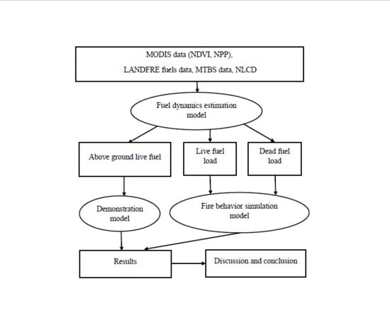
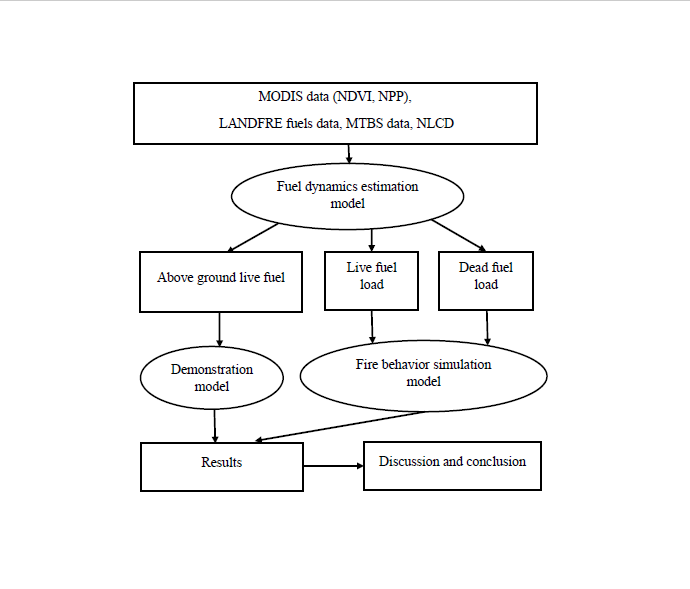
2. Methods
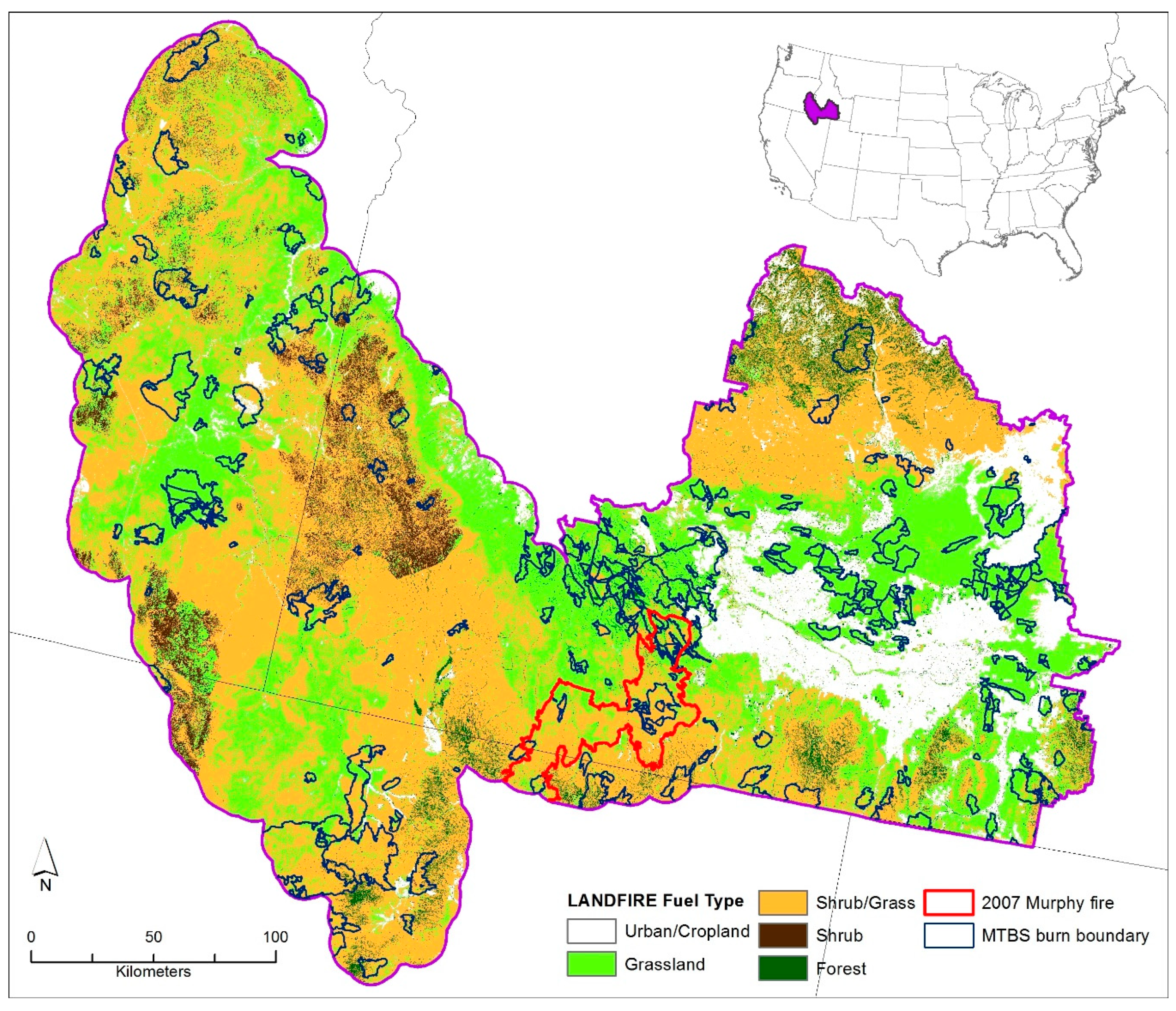
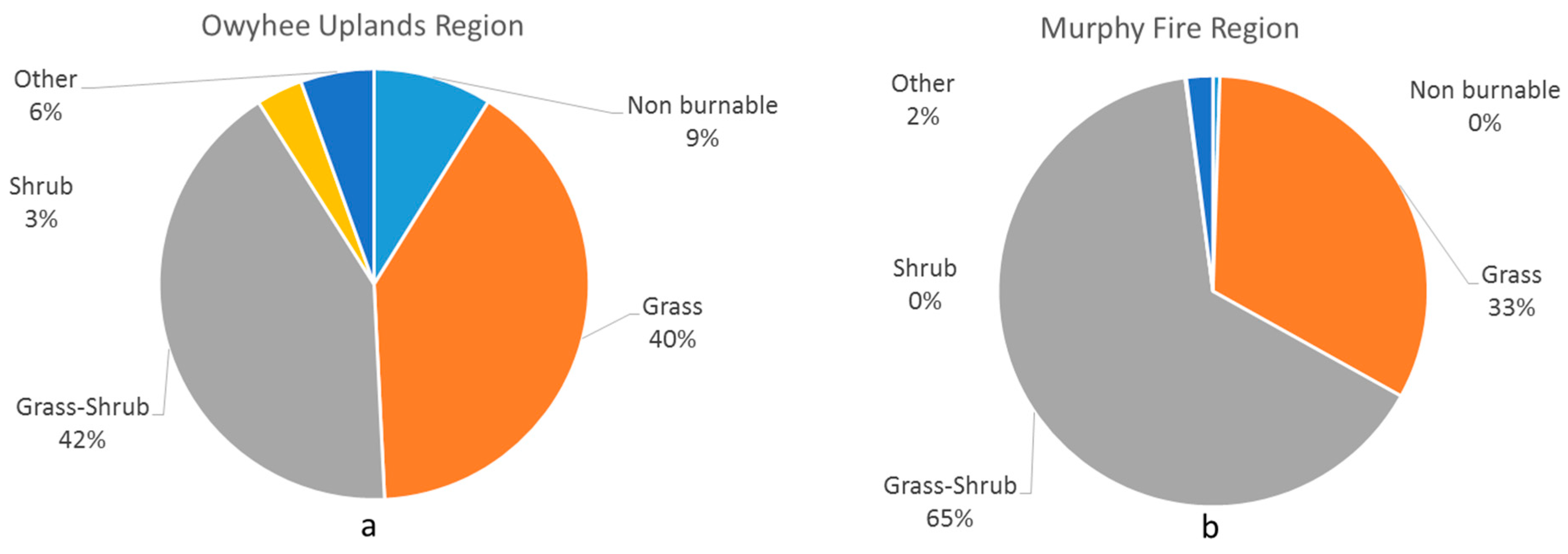
2.1. Study Area
2.2. Fuel Dynamics Estimated from MODIS Products
2.3. Fire Behavior Simulation
- High: fuel parameters were set as the year with high live fuel load (2005)
- Low: fuel parameters were set as the year with low live fuel load (2008)
- Moderate: fuel parameters were set as the year of the Murphy fire (2007)
- Default: fuel parameters were set as the default values from LANDFIRE
3. Results
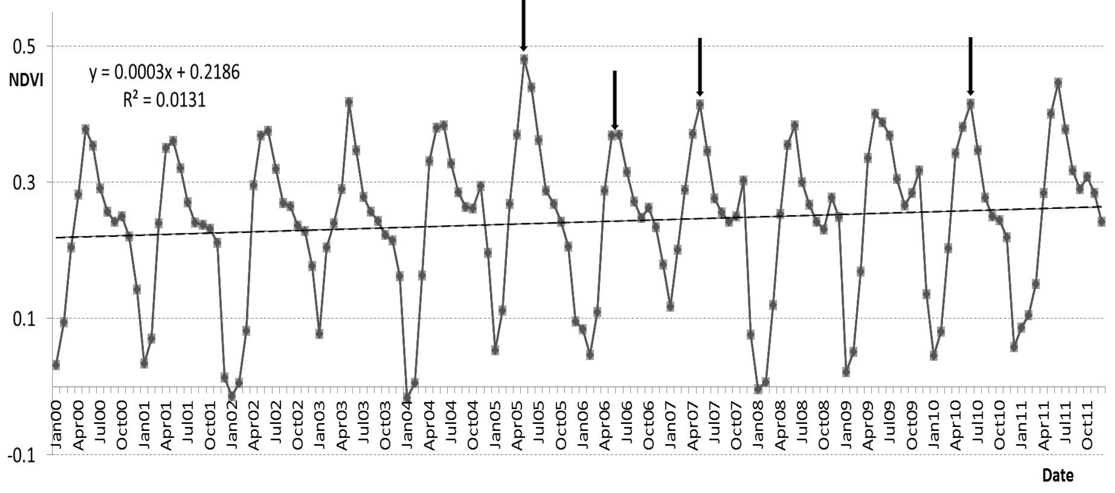
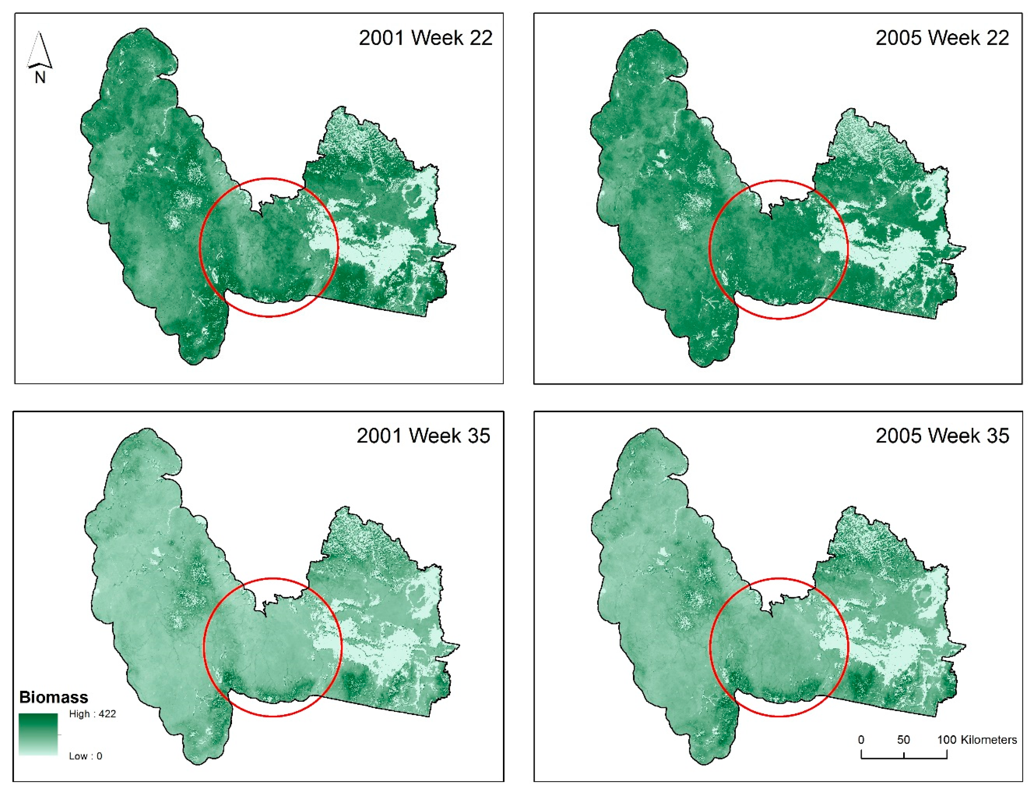
3.1. Fuel Dynamics Estimated from MODIS NDVI Products
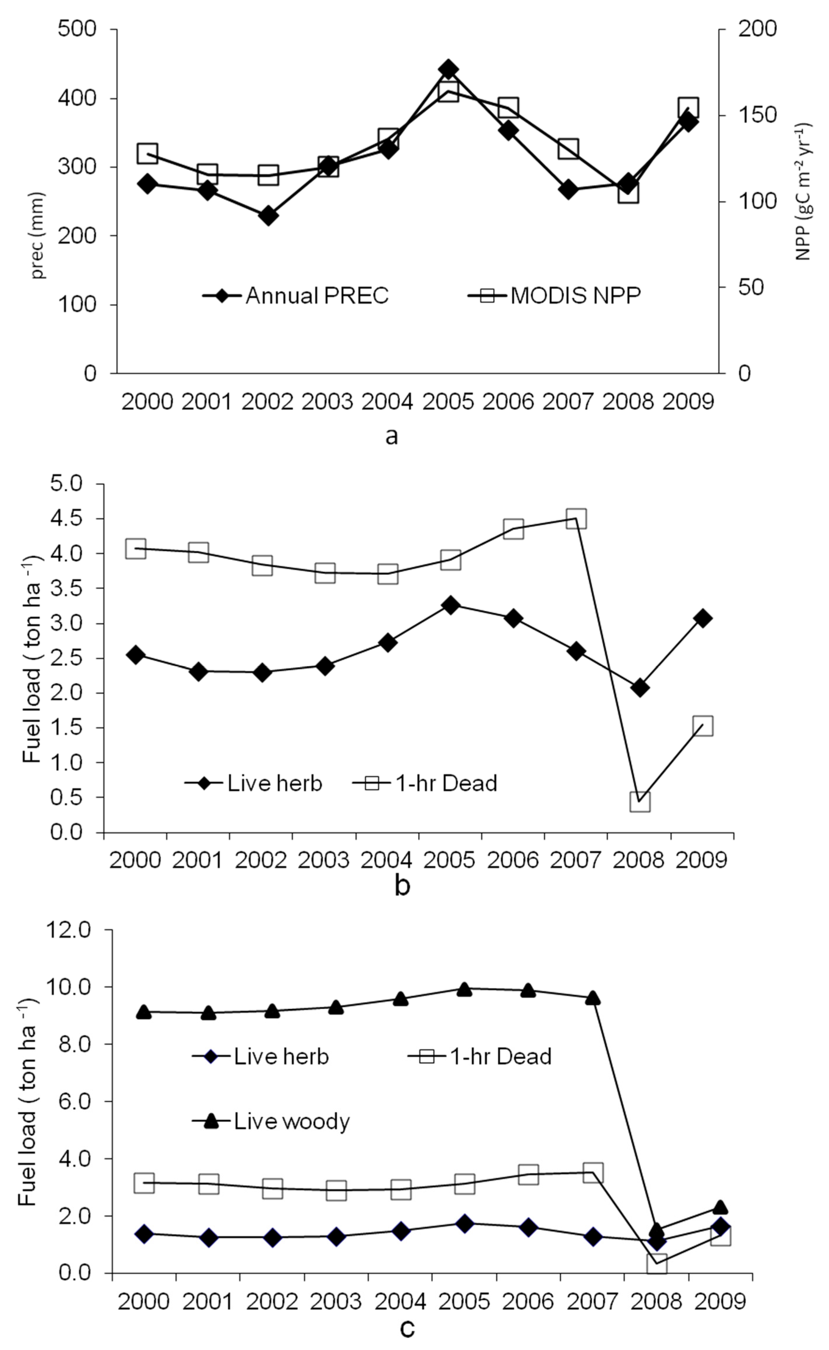
3.2. Fuel Dynamics Estimated from MODIS NPP
3.3. Fire Behavior Simulation
4. Discussion
4.1. Climate Impacts on Shrubland/Grassland Fuel Load Changes
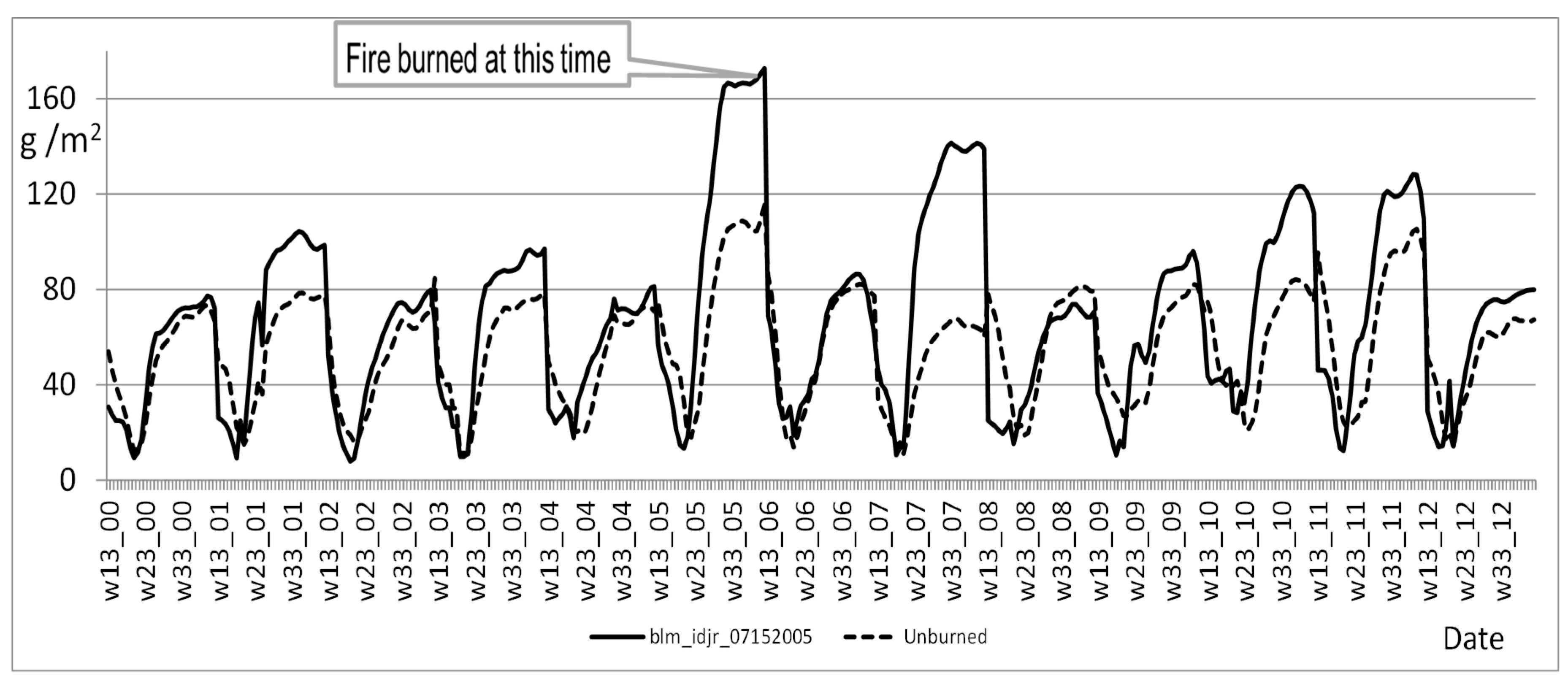
4.2. Fire History Impacts on Shrubland/Grassland Fuel Load
4.3. Using MODIS Products in Fuel Studies
5. Summary
Author Contributions
Funding
Acknowledgments
Conflicts of Interest
References
- Stephens, S.L.; Ruth, L.W. Federal forest-fire policy in the United States. Ecol. Appl. 2005, 15, 532–542. [Google Scholar] [CrossRef] [Green Version]
- Westerling, A.L.; Hidalgo, H.G.; Cayan, D.R.; Swetnam, T.W. Warming and earlier spring increase western U.S. Forest wildfire activity. Science 2006, 313, 940–943. [Google Scholar] [CrossRef] [PubMed] [Green Version]
- Eidenshink, J.; Schwind, B.; Brewer, K.; Zhu, Z.-L.; Quayle, B.; Howard, S. A project for monitoring trends in burn severity. Fire Ecol. 2007, 3, 3–21. [Google Scholar] [CrossRef]
- Program, J.F.S. Joint Fire Science Program. Available online: https://www.firescience.gov/ (accessed on 1 March 2017).
- Rollins, M.G. L: A nationally consistent vegetation, wildland fire, and fuel assessment. Inter. J. Wildland Fire 2009, 18, 235–249. [Google Scholar] [CrossRef] [Green Version]
- LANDFIRE. LANDFIRE Program. Available online: https://www.landfire.gov/ (accessed on 26 April 2017).
- Vogelmann, J.E.; Howard, S.; Rollins, M.G.; Kost, J.R.; Tolk, B.; Short, K.; Chen, X.; Pabst, K.; Huang, C. Monitoring landscape change for landfire using multi-temporal satellite imagery and ancillary data. IEEE J. Sel. Top. Appl. Earth Obs. Remote Sens. 2011, 4, 252–264. [Google Scholar] [CrossRef]
- Burgan, R.E.; Klaver, R.W.; Klarer, J.M. Fuel models and fire potential from satellite and surface observations. Inter. J. Wildland Fire 1998, 8, 159–170. [Google Scholar] [CrossRef]
- Justice, C.O.; Townshend, J.R.G.; Vermote, E.F.; Masuoka, E.; Wolfe, R.E.; Saleous, N.; Roy, D.P.; Morisette, J.T. An overview of MODIS land data processing and product status. Remote Sens. Environ. 2002, 83, 3–15. [Google Scholar] [CrossRef]
- Qi, Y.; Dennison, P.E.; Spencer, J.; Riaño, D. Monitoring live fuel moisture using soil moisture and remote sensing proxies. Fire Ecol. 2012, 8, 71–87. [Google Scholar] [CrossRef]
- Reeves, M.C.; Zhao, M.; Running, S.W. Applying improved estimates of MODIS productivity to characterize grassland vegetation dynamics. Rangel. Ecol. Manag. 2006, 59, 1–10. [Google Scholar] [CrossRef]
- Yebra, M.; Chuvieco, E.; Riaño, D. Estimation of live fuel moisture content from MODIS images for fire risk assessment. Agric. Forest Meteorol. 2008, 148, 523–536. [Google Scholar] [CrossRef]
- Yebra, M.; Dennison, P.E.; Chuvieco, E.; Riaño, D.; Zylstra, P.; Hunt, E.R.; Danson, F.M.; Qi, Y.; Jurdao, S. A global review of remote sensing of live fuel moisture content for fire danger assessment: Moving towards operational products. Remote Sens. Environ. 2013, 136, 455–468. [Google Scholar] [CrossRef]
- Zhang, X.; Friedl, M.A.; Schaaf, C.B.; Strahler, A.H.; Hodges, J.C.F.; Gao, F.; Reed, B.C.; Huete, A. Monitoring vegetation phenology using MODIS. Remote Sens. Environ. 2003, 84, 471–475. [Google Scholar] [CrossRef]
- Roberts, G.; Wooster, M.J.; Xu, W.; He, J. Fire activity and fuel consumption dynamics in sub-saharan Africa. Remote Sens. 2018, 10, 1591. [Google Scholar] [CrossRef] [Green Version]
- Bajocco, S.; Dragozi, E.; Gitas, I.; Smiraglia, D.; Salvati, L.; Ricotta, C. Mapping fuels through vegetation phenology: The role of coarse-resolution satellite time-series. PLoS ONE 2015, 10, e0119811. [Google Scholar] [CrossRef] [PubMed] [Green Version]
- Duff, T.J.; Keane, R.E.; Penman, T.D.; Tolhurst, K.G. Revisiting Wildland Fire Fuel Quantification Methods: The Challenge of Understanding a Dynamic, Biotic Entity. Forests 2017, 8, 351. [Google Scholar] [CrossRef]
- Brown, J.F.; Howard, D.M.; Wylie, B.K.; Friesz, A.M.; Ji, L.; Gacke, C. Application-ready expedited modis data for operational land surface monitoring of vegetation condition. Remote Sens. 2015, 7, 16226–16240. [Google Scholar] [CrossRef] [Green Version]
- USDA. Major Land Resource Regions Custom Report (USDA Agriculture Handbook 296). Available online: https://www.nrcs.usda.gov/wps/portal/nrcs/main/soils/survey/ (accessed on 22 October 2017).
- MTBS. Monitoring Trends in Burn Severity. Available online: https://www.mtbs.gov/ (accessed on 1 August 2017).
- Launchbaugh, K.; Brammer, B.; Brooks, M.; Bunting, S.; Clark, P.; Davison, J.; Fleming, M.; Kay, R.; Pellant, M.; Pyke, D.; et al. Interactions among Livestock Grazing, Vegetation Type, and Fire Behavior in the Murphy Wildland Fire Complex in Idaho and Nevada; U.S. Geological Survey: Fort Collins, CO, USA, 2008.
- Scott, J.; Burgan, R.; Robert, E. Standard Fire Behavior Fuel Models: A Comprehensive Set for Use with Rothermel’s Surface Fire Spread Model; U.S. Department of Agriculture, Forest Service, Rocky Mountain Research Station: Fort Collins, CO, USA, 2005.
- Cleary, M.B.; Pendall, E.; Ewers, B.E. Aboveground and belowground carbon pools after fire in mountain big sagebrush steppe. Rangel. Ecol. Manag. 2010, 63, 187–196. [Google Scholar] [CrossRef]
- Davies, K.W.; Bates, J.D.; Miller, R.F. Short-term effects of burning Wyoming big sagebrush steppe in southeast Oregon. Rangel. Ecol. Manag. 2007, 60, 515–522. [Google Scholar] [CrossRef]
- Wright, C.; Prichard, S. Biomass Consumption during Prescribed Fires in Big Sagebrush Ecosystems; U.S. Department of Agriculture, Forest Service: Washington, DC, USA, 2006; pp. 489–500.
- Gamon, J.A.; Field, C.B.; Goulden, M.L.; Griffin, K.L.; Hartley, A.E.; Joel, G.; Penuelas, J.; Valentini, R. Relationships between NDVI, canopy structure, and photosynthesis in three Californian vegetation types. Ecol. Appl. 1995, 5, 28–41. [Google Scholar] [CrossRef] [Green Version]
- Chapin III, F.S.; Woodwell, G.M.; Randerson, J.T.; Rastetter, E.B.; Lovett, G.M.; Baldocchi, D.D.; Clark, D.A.; Harmon, M.E.; Schimel, D.S.; Valentini, R.; et al. Reconciling carbon-cycle concepts, terminology, and methods. Ecosyst. 2006, 9, 1041–1050. [Google Scholar] [CrossRef] [Green Version]
- Scurlock, J.M.O.; Johnson, K.; Olson, R.J. Estimating net primary productivity from grassland biomass dynamics measurements. Glob. Change Biol. 2002, 8, 736–753. [Google Scholar] [CrossRef] [Green Version]
- Running, S.W.; Nemani, R.R.; Heinsch, F.A.; Zhao, M.; Reeves, M.; Hashimoto, H. A continuous satellite-derived measure of global terrestrial primary production. BioSci. 2004, 54, 547–560. [Google Scholar] [CrossRef]
- Prince, S.D.; Goward, S.N. Global primary production: A remote sensing approach. J. Biogeogr. 1995, 22, 815–835. [Google Scholar] [CrossRef]
- Heinsch, F.; Reeves, M.; Votava, P.; Kang, S.; Milesi, C.; Zhao, M.; Glassy, J.; Jolly, W.; Loehman, R.; Bowker, C.; et al. User’s Guide on GPP and NPP (mod17a2/a3) Products NASA MODIS Land Algorithm. Version 2.0; University of Montana: Missoula, MT, USA, 2003. [Google Scholar]
- Zhao, M.; Heinsch, F.A.; Nemani, R.R.; Running, S.W. Improvements of the MODIS terrestrial gross and net primary production global data set. Remote Sens. Environ. 2005, 95, 164–176. [Google Scholar] [CrossRef]
- NTSG. Numerical Terradynamic Simulation Group (NTSG). Available online: ftp://ftp.ntsg.umt.edu/pub/MODIS/NTSG_Products/ (accessed on 1 August 2013).
- Zhao, M.; Running, S.W. Drought-induced reduction in global terrestrial net primary production from 2000 through 2009. Science 2011, 334, 1496. [Google Scholar] [CrossRef] [Green Version]
- Running, S.W.; Coughlan, J.C. A general model of forest ecosystem processes for regional applications i. Hydrologic balance, canopy gas exchange and primary production processes. Ecol. Model. 1988, 42, 125–154. [Google Scholar] [CrossRef]
- Thornton, P.E.; Law, B.E.; Gholz, H.L.; Clark, K.L.; Falge, E.; Ellsworth, D.S.; Goldstein, A.H.; Monson, R.K.; Hollinger, D.; Falk, M.; et al. Modeling and measuring the effects of disturbance history and climate on carbon and water budgets in evergreen needleleaf forests. Agric. Forest Meteorol. 2002, 113, 185–222. [Google Scholar] [CrossRef]
- White, M.; Thornton, P.; Running, S.; Nemani, R. Parameterization and sensitivity analysis of the biome-BGC terrestrial ecosystem model: Net primary production controls. Earth Interact. 2000, 4, 1–85. [Google Scholar] [CrossRef]
- Miller, R.F.; Schultz, L.M. Development and longevity of ephemeral and perennial leaves on Artemisia tridentata Nutt. ssp. wyomingensis. Great Basin Nat. 1987, 47, 227–230. [Google Scholar]
- Perfors, T.; Harte, J.; Alter, S.E. Enhanced growth of sagebrush (Artemisia tridentata) in response to manipulated ecosystem warming. Glob. Change Biol. 2003, 9, 736–742. [Google Scholar] [CrossRef]
- Kemp, P.R.; Reynolds, J.F.; Virginia, R.A.; Whitford, W.G. Decomposition of leaf and root litter of Chihuahuan desert shrubs: Effects of three years of summer drought. J. Arid Environ. 2003, 53, 21–39. [Google Scholar] [CrossRef]
- Knorr, M.; Frey, S.D.; Curtis, P.S. Nitrogen additions and litter decomposition: A meta-analysis. Ecology 2005, 86, 3252–3257. [Google Scholar] [CrossRef]
- Shaw, M.R.; Harte, J. Control of litter decomposition in a subalpine meadow-sagebrush steppe ecotone under climate change. Ecol. Appl. 2001, 11, 1206–1223. [Google Scholar]
- Throop, H.L.; Archer, S.R. Interrelationships among shrub encroachment, land management, and litter decomposition in a semidesert grassland. Ecol. Appl. 2007, 17, 1809–1823. [Google Scholar] [CrossRef] [PubMed]
- Zhu, Z.; Bergamaschi, B.; Bernknopf, R.; Clow, D.; Dye, D.; Faulkner, S.; Forney, W.; Gleason, R.; Hawbaker, T.; Liu, J.; et al. A Method for Assessing Carbon Stocks, Carbon Sequestration, and Greenhouse-Gas Fluxes in Ecosystems of the United States under Present Conditions and Future Scenarios; U.S. Geological Survey: Washington, DC, USA, 2010.
- Andrews, P.; Bevins, C.; Seli, R. BehavePlus Fire Modeling System, Version 4.0: User’s Guide; U.S. Department of Agriculture, Forest Service, Rocky Mountain Research Station: Fort Collins, CO, USA, 2008.
- Bradshaw, L.; Deeming, J.; Burgan, R. The 1978 National Fire-Danger Rating System; U.S. Department of Agriculture Forest Service, Intermountain Forest and Range Experiment Station: Ogden, UT, USA, 1978.
- Burgan, R. 1988 Revisions to the 1978 National Fire-Danger Rating System; U.S. Department of Agriculture Forest Service, Southeastern Forest Experiment Station: Asheville, NC, USA, 1988.
- Deeming, J.; Burgan, R.; Cohen, J. The National Fire-Danger Rating System-1978; U.S. Department of Agriculture Forest Service, Intermountain Forest and Range Experiment Station: Ogden, UT, USA, 1977.
- Finney, M. FARSITE: Fire Area Simulator–Model Development and Evaluation; Department of Agriculture, Forest Service, Rocky Mountain Research Station: Ogden, UT, USA, 2004.
- DRI. Historical Fire Weather Data for FPA. Desert Research Institute. Available online: https://wrcc.dri.edu/fpa/ (accessed on 1 March 2015).
- IPCC. Climate Change 2013: The Physical Science Basis; Intergovernmental Panel on Climate Change, Cambridge University Press: Cambridge, UK; New York, NY, USA, 2013. [Google Scholar]
- Baeza, M.J.; De Luís, M.; Raventós, J.; Escarré, A. Factors influencing fire behaviour in shrublands of different stand ages and the implications for using prescribed burning to reduce wildfire risk. J. Environ. Manag. 2002, 65, 199–208. [Google Scholar] [CrossRef] [PubMed]
- Cooper, S.; Lesica, P.; Kudray, G. Post-Fire Recovery of Wyoming Big Sagebrush Shrub-Steppe in Central and Southeast Montana; The United States Department of the Interior, Bureau of Land Management, State Office: Helena, MT, USA, 2007.
- West, N.; Hassan, M. Recovery of sagebrush-grass vegetation following wildfire. Rangel. Ecol. Manag. 1985, 38, 131–134. [Google Scholar]
- Gao, F.; Masek, J.; Schwaller, M.; Hall, F. On the blending of the Landsat and MODIS surface reflectance: Predicting daily Landsat surface reflectance. IEEE Trans. Geosci. Remote Sens. 2006, 44, 2207–2218. [Google Scholar]
- Zhang, X.; Wang, J.; Henebry, G.M.; Gao, F. Development and evaluation of a new algorithm for detecting 30 m land surface phenology from VIIRS and HLS time series. ISPRS J. Photogramm. Remote Sens. 2020, 161, 37–51. [Google Scholar] [CrossRef]
- Zhu, X.; Chen, J.; Gao, F.; Chen, X.; Masek, J.G. An enhanced spatial and temporal adaptive reflectance fusion model for complex heterogeneous regions. Remote Sens. Environ. 2010, 114, 2610–2623. [Google Scholar] [CrossRef]
- Gao, F. Integrating Landsat with MODIS products for vegetation monitoring. In Satellite-Based Applications on Climate Change; Qu, J., Powell, A., Sivakumar, M.V.K., Eds.; Springer: Dordrecht, The Netherlands, 2013; pp. 247–261. [Google Scholar]
- Homer, C.; Dewitz, J.; Fry, J.; Coan, M.; Hossain, N.; Larson, C.; Herold, N.; McKerrow, A.; VanDriel, J.N.; Wickham, J. Completion of the 2001 national land cover database for the conterminous United States. Photogramm. Eng. Remote Sens. 2007, 73, 337–341. [Google Scholar]


| Fuel Type | Fuel LOAD | Fuel loads (ton ha−1) | ||||
|---|---|---|---|---|---|---|
| Live Herbaceous | Live Woody | 1-Hour Dead | ERC 1 (KJ m−2) | FL 2(m) | ||
| Grass | High (2005) | 3.27 | 0 | 3.92 | 10425 | 3.41 |
| Grass | Moderate (2007) | 2.6 | 0 | 4.5 | 10209 | 3.38 |
| Grass | Low (2008) | 2.08 | 0 | 0.45 | 3043 | 1.95 |
| Grass | Default (GR2) | 2.24 | 0 | 0.22 | 2953 | 1.92 |
| Shrub | High (2005) | 1.75 | 9.95 | 3.12 | 20043 | 3.23 |
| Shrub | Moderate (2007) | 1.3 | 9.64 | 3.52 | 19544 | 3.23 |
| Shrub | Low (2008) | 1.14 | 1.52 | 0.36 | 3770 | 1.58 |
| Shrub | Default (GS2) | 1.34 | 2.24 | 1.12 | 6348 | 2.16 |
| Live Fuel Load | Area Burned (ha) |
|---|---|
| High (2005) | 33,998 |
| Moderate (2007) | 35,386 |
| Low (2008) | 32,937 |
| Default | 48,593 |
© 2020 by the authors. Licensee MDPI, Basel, Switzerland. This article is an open access article distributed under the terms and conditions of the Creative Commons Attribution (CC BY) license (http://creativecommons.org/licenses/by/4.0/).
Share and Cite
Li, Z.; Shi, H.; Vogelmann, J.E.; Hawbaker, T.J.; Peterson, B. Assessment of Fire Fuel Load Dynamics in Shrubland Ecosystems in the Western United States Using MODIS Products. Remote Sens. 2020, 12, 1911. https://doi.org/10.3390/rs12121911
Li Z, Shi H, Vogelmann JE, Hawbaker TJ, Peterson B. Assessment of Fire Fuel Load Dynamics in Shrubland Ecosystems in the Western United States Using MODIS Products. Remote Sensing. 2020; 12(12):1911. https://doi.org/10.3390/rs12121911
Chicago/Turabian StyleLi, Zhengpeng, Hua Shi, James E. Vogelmann, Todd J. Hawbaker, and Birgit Peterson. 2020. "Assessment of Fire Fuel Load Dynamics in Shrubland Ecosystems in the Western United States Using MODIS Products" Remote Sensing 12, no. 12: 1911. https://doi.org/10.3390/rs12121911