Toward the Detection of Permafrost Using Land-Surface Temperature Mapping

Abstract

Permafrost is degrading under current warming conditions, disrupting infrastructure, releasing carbon from soils, and altering seasonal water availability. Therefore, it is important to quantitatively map the change in the extent and depth of permafrost. We used satellite images of land-surface temperature to recognize and map the zero curtain, i.e., the isothermal period of ground temperature during seasonal freeze and thaw, as a precursor for delineating permafrost boundaries from remotely sensed thermal-infrared data. The phase transition of moisture in the ground allows the zero curtain to occur when near-surface soil moisture thaws or freezes, and also when ice-rich permafrost thaws or freezes. We propose that mapping the zero curtain is a precursor to mapping permafrost at shallow depths. We used ASTER and a MODIS-Aqua daily afternoon land-surface temperature (LST) timeseries to recognize the zero curtain at the 1-km scale as a “proof of concept.” Our regional mapping of the zero curtain over an area around the 7000 m high volcano Ojos del Salado in Chile suggests that the zero curtain can be mapped over arid regions of the world. It also indicates that surface heterogeneity, snow cover, and cloud cover can hinder the effectiveness of our approach. To be of practical use in many areas, it may be helpful to reduce the topographic and compositional heterogeneity in order to increase the LST accuracy. The necessary finer spatial resolution to reduce these problems is provided by ASTER (90 m).

1. Introduction

Permafrost, defined as ground that stays below freezing for more than two years, is an integral part of the cryosphere that is predicted to rapidly degrade under current warming climatic conditions (e.g., [1,2]). A quarter of the land surface of the Earth is subject to permafrost-related processes [3] and 23–26% of the land area in the northern hemisphere is permafrost [4,5,6]. The loss of permafrost affects the regional water balance and changes landscapes and ecosystems in cold regions. Erosion of soil due to melting permafrost not only poses a significant uncertainty in infrastructure stability but may also accelerate the release of carbon from the permafrost into the atmosphere [1,7].

Traditional mapping and monitoring techniques of permafrost are accurate but are presently labor-intensive and rely on interpolating small numbers of locally measured data across large areas in order to study regional-scale processes. Remote sensing addresses this difficulty by making spatially dense measurements over vast regions. Previous remote sensing studies have inferred permafrost extent from the instantaneous zero isotherm at the land surface or from changes in the dielectric marking the phase transition of liquid water to ice [8,9,10].

We propose to use land-surface temperature (LST) measured from space-borne thermal-infrared (TIR) sensors to map patterns in the annual cycle of LST in order to ultimately detect freeze/thaw surface dynamics. Previous studies demonstrated that in autumn or spring, the LST of moist/frozen soils remains at ~0 °C while the phase transition between water and ice occurs. This period is a well-known phenomenon called the “zero curtain” in permafrost studies (e.g., [11]) and its presence can be used to distinguish seasonally freezing ground from freezing dry ground, in which there is no zero curtain. The premise of our approach is that if the zero curtain lasts for several days, its presence can potentially be recognized and mapped with time series of daily LST images.

Repetition of the zero curtain for two or more annual LST cycles can be used to identify candidate permafrost pixels, and seasonal asymmetry in the duration of the zero curtain can likely be used to distinguish seasonally frozen soil from permafrost. Putkonen [12] suggested from modeling, substantially confirmed by Yi et al. [13], that the zero curtain should be present over near-surface permafrost during freeze-up, but not during the thaw, and vice versa in seasonally frozen soil. Over deep permafrost (~130 cm), de Pablo et al. [14] reported zero curtains in both seasons but shorter at the end of the freezing season. Although the zero-curtain duration is affected by seasonal changes in soil moisture and by the onset date of snow cover [13], this asymmetry should allow further winnowing of candidate pixels.

This paper does not reach so far as to identify permafrost, but simply establishes that precursor maps of the zero curtain are feasible to make with satellite-borne TIR imagers. We tested our approach in an arid region of the Atacama Andes near the Ojos del Salado volcano, close to the border between Chile and Argentina, where previous studies had documented the presence of frozen ground and near-surface permafrost [15,16,17,18].

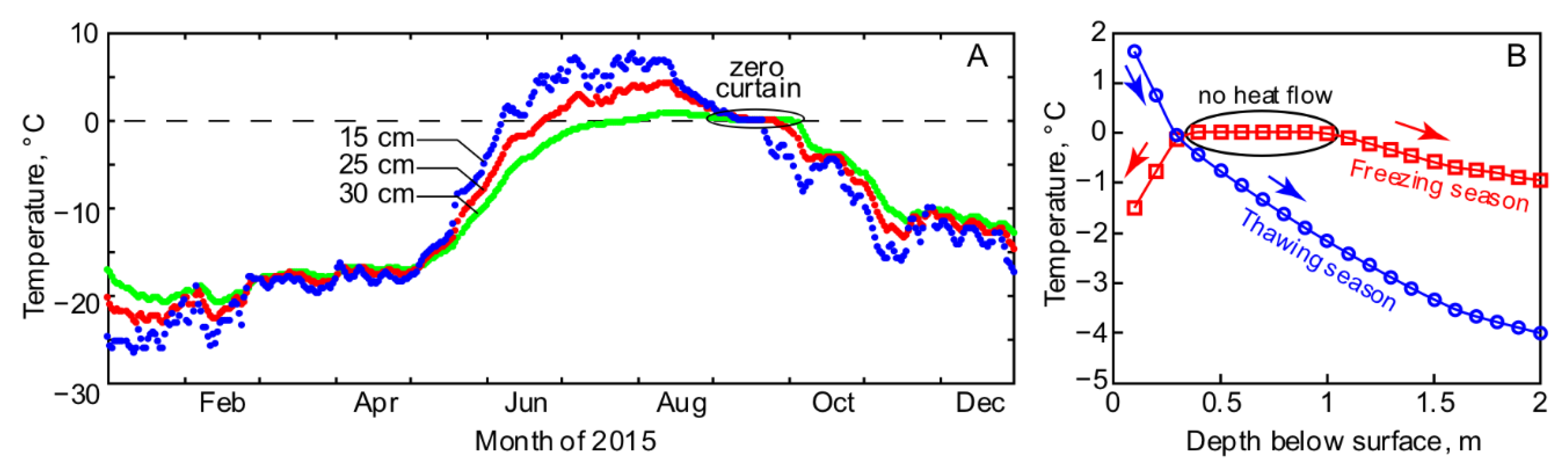
1.1. Zero Curtain in the Surface and Soil Temperatures

The occurrence of a zero curtain in the annual ground-temperature cycle is attributed to the phase change of moisture in the soil due to the release of excess latent heat during the freezing and thawing seasons (Figure 1). Because keeping soil near 0 °C for several days generally requires moisture in the soil, the detection of the zero curtain implies the presence of soil moisture. Soil moisture may be ephemeral or seasonal, but it may further imply the presence of buried ice-rich permafrost. Putkonen [12] proposed that, in addition to the presence of moisture in the soil, the thermal gradient in the soil must become 0 °C m⁻¹ above the base of the active layer (depth of the thaw) for the zero curtain to form. It follows that the timing of the zero curtain indicates the presence of permafrost. During the thaw season, a high thermal gradient between the warming surface and the cold permafrost effectively conducts heat through the soil without forming a zero curtain; during freeze-up, the cold ground surface and the cold permafrost create a low thermal gradient, ensuring a condition at some depth in the soil where the temperature is at or near 0 °C for a prolonged period (Figure 1B). In other words, seasonally frozen ground not overlying permafrost may exhibit a zero curtain during the thaw, whereas soil underlain by permafrost may exhibit a zero curtain only during freeze-up.

Yi et al. [13] observed that the duration of the zero curtain revealed information about the permafrost, specifically the depth of the active layer. The heat-flow plateau at ~0 °C shown schematically in Figure 1B (from Putkonen [12]) would persist longer over thicker active layers but would break down more rapidly over thin layers. Measuring and mapping the duration of the zero curtain, therefore, would supply important information about the weather conditions, their change with altitude and geographic position, and changes over time relevant to climate change.

Significant characteristics of the zero curtain may be measured by three parameters: (1) The starting date of the zero curtain; (2) the duration of the zero curtain; and (3) seasonal asymmetry in the duration. While the zero curtain itself indicates the presence of soil moisture, its starting date reveals the beginning of the annual thaw and/or freeze-up and its change over the years may indicate the changing nature of the climate and seasonal fluctuations of soil moisture. The duration of the zero curtain may respond to the thermal regime of the soil and the presence of underlying permafrost and the depth of the active layer.

The analysis of daily measurements of LST is less sensitive to measurement precision and cloud cover than a single measurement of LST. The occurrence of the zero curtain in LST, regardless of the seasons, strongly indicates the presence of moisture in the soil and provides an opportunity to distinguish between dry and wet soil and map at a regional scale. Therefore, such a remote-sensing approach may be appropriate for detecting and mapping ground ice at moderate (10²–10³ m) resolutions.

1.2. Remote Sensing and Numerical Modeling Studies of Permafrost

Most of the traditional permafrost studies rely on the recognition of landscape changes in the field and extrapolating over large regions (e.g., [19]). Such field expeditions can be expensive and prohibitive in remote regions. If the changes in the landscape are large enough to be seen with remotely sensed data, the permafrost-related landscapes and their changes can be mapped at a regional scale. For example, Nitze et al. [20] used visible/near-infrared Landsat imagery (30 m resolution) from 1999 to 2014 to quantify the expansion of thermokarst lakes and the increased slumping of frozen coastal areas due to melting of permafrost. Such studies are invaluable to document landscape changes in permafrost areas but are not sufficient to explain the changes in the thermal regime of the soil.

Microwave sensors are sensitive to soil moisture and temperature (e.g., [21]), and exploiting the fact that freezing changes the dielectric constant of moist soils, numerous studies of radar measurements have been used to map the state of freeze and thaw in the soils (e.g., [22,23]). Such regional-scale mapping approaches based on microwave sensors are useful to infer the changes in seasonally frozen grounds. However, the existence of permafrost underlying the seasonally frozen ground has not been inferred from just the dielectric constant or the state of freeze/thaw, and the resolution of the microwave sensors (~6–60 km) can be a limiting factor to detect small changes in lateral extent of permafrost areas. With the goal of mapping the depth of the active layer, Liu et al. [24] used interferometric synthetic aperture radar (InSAR) to monitor surface deformation over permafrost. Because ice and water have different densities, the ground surface settles during the thaw and the amount of surface subsidence can be used to estimate the thickness of the active layer if the vertical distribution of pore water within the soil is known. Wang et al. [25] used multi-temporal TerraSAR-X backscatter intensity and interferometric coherence along with the relationship between vegetation cover and the permafrost as the basis for classifying and mapping permafrost landscape features. Chen et al. [26] proposed a method to estimate the active layer thickness using time-series P-band polarimetric synthetic aperture radar (SAR) observations, achieving retrieval with errors <0.1 m in some cases. Yi et al. [13] combined field observations, active layer thickness, and soil moisture maps derived from low-frequency (L + P-band) airborne radar measurements, and global satellite environmental observations to investigate the sensitivity of the active layer to recent climate trends.

Thermal infrared (TIR) sensors provide direct measurements of skin temperatures of land surfaces. Widely used LST products are derived from the Advanced Spaceborne Thermal Emission and Reflection Radiometer (ASTER) onboard the Terra spacecraft, the Thematic Mapper (onboard Landsat), and from the Moderate Resolution Imaging Spectroradiometer (MODIS) onboard two satellites: Terra (with a morning overpass) and Aqua (with an afternoon overpass). Terra, Landsat, and Aqua share a common sun-synchronous orbit with different overpass times. Among the TIR imagers on these satellites, only MODIS provides daily measurements of LST. Numerical modeling studies based on the empirical relationship between the ground temperature and air temperature have taken advantage of the MODIS LST products (e.g., [27,28,29]) to derive static maps of the spatial distribution of permafrost. Recently, a numerical modeling study has combined the MODIS LST products with gridded air temperature data to derive time-series maps of permafrost extent [5]. These dynamic maps of changes in permafrost are important to assess the impact of a warming climate to the state of the permafrost. The approach proposed in this article is a contribution toward creating temporally and spatially dynamic maps of the quantified state of permafrost and seasonally frozen ground, complementary to the previous regional-scale studies.

2. Materials and Methods

2.1. Remotely Sensed and Climate Data

MODIS provides daily LST products (MOD11A1 and MYD11A1) at 1-km spatial resolution using TIR data measured from the Aqua and Terra platforms, respectively [30,31]. We used MYD11A1 (Aqua) daytime LST products from 2003 to 2017. The MODIS LST is estimated using the split-window algorithm [32] with an estimated uncertainty of ~4.5 °C [33]. We compiled the daily MODIS LST over the study area and converted the data for processing with MATLAB. Daily coverage is possible using oblique views from adjacent overpasses. The local time for MODIS measurements in the LST compilations, therefore, ranged from 1:10 to 2:50 PM.

We used an ASTER Surface Kinetic Temperature (AST_08; 90 m pixel⁻¹) and visible/near-infrared (VNIR) ASTER products (AST_L1B; 15 m pixel⁻¹) to assess the variability of the land surface and the related temperatures within a single MODIS pixel, and to check the distribution of snow. The ASTER products were derived from a scene acquired on 8 April, 21 August, 22 September, and 8 October of 2017 at 11:43 AM local time [34].

Air temperature variations over different altitudes were evaluated using the long-term (1981–2010) monthly mean air temperature data from the Global Historical Climatology Network and Climate Anomaly Monitoring System (GHCN CAMS; 0.5° pixel⁻¹ [35]). These low-resolution air temperature data were resampled at a 30 m pixel⁻¹ resolution using the SRTM 1 arc-second DEM [36] and the long-term (1981–2010) monthly mean lapse rate derived from the National Centers for Environmental Prediction and the National Center for Atmospheric Research reanalysis data (NCEP/NCAR; 2.5° pixel⁻¹ [37]). We followed the procedures described in [38] to resample the air temperature data to a higher spatial resolution to see the fine spatial variations of air temperature.

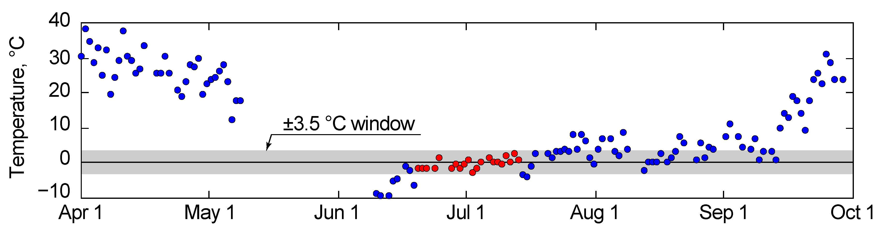
2.2. “Threshold Window” Filtering Algorithm

We developed an algorithm in the MATLAB environment that analyzes the daily MODIS LST during the first and second six months of the year at each pixel, and tests whether the daily LST satisfies the following rules indicating the occurrence of a zero curtain:

(1)

LST must be between −3.5 and 3.5 °C (defined below as the LST during a zero-curtain event, or “zero-curtain LST”);

(2)

The number of consecutive zero-curtain LSTs must be >3;

(3)

The number of days with missing data between two identified zero-curtain LSTs must be <3; and

(4)

The total number of zero-curtain LSTs must be >5.

In other words, we split the annual daily LST data into two halves, each containing the thaw or freeze-up period. In each half, we counted the number days during which the −3.5 < LST < 3.5 °C. We identified a zero curtain if the number of consecutive days with −3.5 < LST < 3.5 °C exceeded five. At the end of the counting iteration for a pixel, the starting and end date for the zero curtain were recorded, from which we calculated the difference, which we defined as the duration of the zero curtain. Currently, no correction is made for snow cover. Our algorithm returns as output for every pixel matrix for the zero-curtain duration and the starting dates for thawing and freezing seasons for each year. The output matrix was converted back to georeferenced raster files using the same gridding scheme and spatial resolution of MYD11A1 products. All maps and raster data produced from this study are available in georeferenced TIFF files, as well as the detailed descriptions of the data, in the online supplement to this article (Table S1).

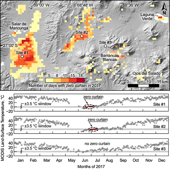
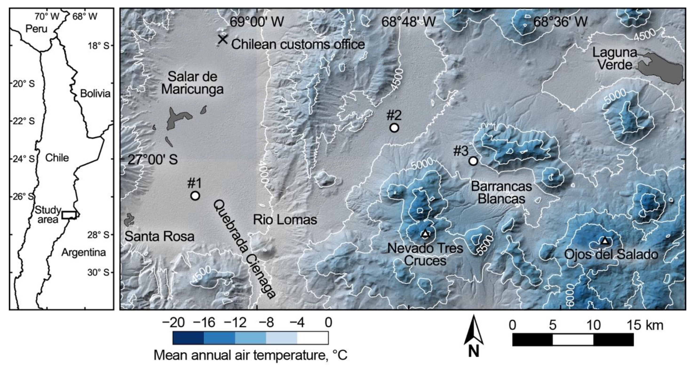
2.3. Validation Sites

We chose three validation sites near the Ojos del Salado volcano in the Andes east of the Atacama Desert in Chile (Figure 2). At least one 1-km² area surrounding each study site is homogeneous in terms of composition and small-scale roughness, topographically flat, and sparsely vegetated. Climate data are given in

Table 1. Validation sites, their locations, and local climate. Precipitation data are too low resolution to show differences among the sites.

Site	Location	Altitude, m asl	Mean Annual Climate Parameters
			Precipitation 1, mm w.e.	Air Temperature 2, °C	Lapse Rate 3, °C km−1
#1	27°02′54” S, 69°04′52″ W	3815	58	−0.8	5.5
#2	26°57′31” S, 68°49′09″ W	4415	58	−3.1	5.5
#3	27°00′09” S, 68°42′55″ W	4910	58	−5.0	6.3

¹ All sites show the same precipitation due to 0.5° resolution of GPCC V7 data [42]; ² [35]; ³ [37].

. Only ~1% of the total surface area over the whole region including the validation sites is covered with shrubs, grassland, water bodies, and permanent snowfields or glaciers (supplementary Table S2). Two of the sites were chosen in areas that were previously found to have periglacial features [39] and possibly permafrost [16,40]. However, intermittent or thin snow cover on Ojos del Salado implies complicating factors due to increased soil moisture during the melt season and the possibility of near-surface ground ice. The sites were chosen at different altitudes, ranging from 3815 to 4910 m asl, to assess the variability in the zero curtain at various altitudes. The lowest site lacked periglacial features and was intended to act as control for the higher ones.

Site #1 is located on one of the low-gradient (1°) alluvial fans (~140 km²) emanating from the rivers Quebrada Cienaga and Rio Lomas (Figure 2). These rivers form braided channels that lead to Salar de Maricunga, but the channels remain dry most of the time. The surface of the fan is paved with rhyodacitic/andesitic (cf. Baker et al. [41]) gravel 2–3 cm in diameter and 1 cm thick, overlying silty sand. A few of the clasts are 3–5 cm in diameter and <2 cm thick. Site #2 is located on an alluvial fan (~13 km²) below the volcanoes Nevado Tres Cruces. The surface of this fan is a low-gradient (~2°) rhyodacitic/andesitic/dacitic gravel pavement similar to Site #1, with gravel 2 cm in diameter and 1 cm thick. Site #3 (~1 km²) is on a steeper alluvial fan (~10%) in the Valle de Barrancas Blancas and has the most complex surface in terms of composition (pyroclastic, rhyolitic, dacitic) and topography. It is covered with gravel 3–5 cm in diameter and <3 cm thick. Some large wind-polished boulders are scattered on the surface. Almost-parallel, shallow, dry channels ~20 cm deep dissect the surface. Small grasses and flowers may cover the site in summer. At all three sites, the percent of the surface covered by gravel was >90%. Photos showing the surface features at the validation sites are provided in supplementary Figures S1–S7.

Surface features in the study region indicate periglacial processes and seasonal freeze and thaw. For example, in the Valle de Barrancas Blancas (Figure 2), sorted and unsorted patterned ground, surface extrusion due to cryoturbation, rock glaciers, cryoplanation surfaces, and slopes affected by gelifluction have been observed by Buchroithner and Trombotto Liaudat [43]. Nagy et al. [16] measured ground temperatures at six sites at different altitudes, ranging from 4200 to 6890 m asl, around Ojos del Salado during 2012–2016 to show that the seasonal freezing front reaches depths of at least 35–60 cm at these altitudes. Zero curtains were observed in both spring and autumn for two more weeks at all six sites, except for the two highest sites, at 6750 and 6890 m asl, where the ground temperatures remained below 0 °C for most of the year (see Section 2.4 below). On the basis of these measured ground temperatures, Nagy et al. [16] concluded that permafrost likely exists above 5250 m asl. The likelihood of permafrost at these altitudes is consistent with suggestions based on the mapping of permafrost and periglacial landforms [39,44] and numerical modeling of air temperatures [40]. Nagy et al. [16] concluded that it is unlikely for permafrost to exist below 4550 m asl.

2.4. In-Situ Measurements at Validation Sites

In November 2016, we installed TMC6-HC temperature sensors with an accuracy of ±0.25 °C at each site to measure subsurface ground temperatures every hour at depths of 2, 10, 20, and 40 cm (Figure 2; Table 1). The data from the thermometers were collected using HOBO^® H-8 4-channel data loggers. The near-surface sensor was for comparison to the MODIS LST data, averaged over 1 km². The deeper subsurface sensors were to evaluate the 2-cm temperature in terms of the diurnal cycle. When we removed the probes (March 2018), we examined the soils. See soil descriptions at Site #1 (Table S3), at Site #2 (Table S4), and at Site #3 (Table S5) in the online Supplementary Materials.

3. Results

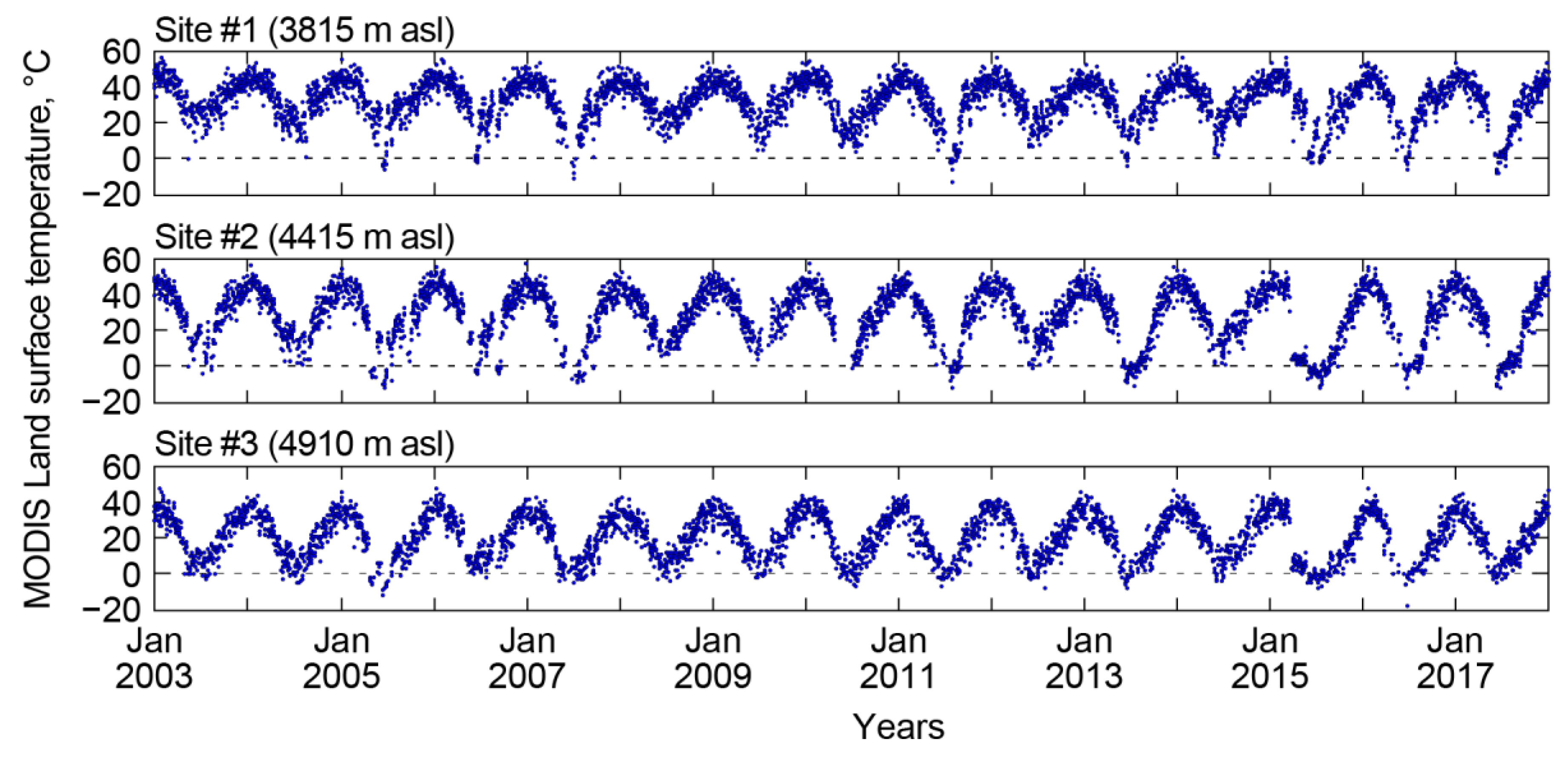
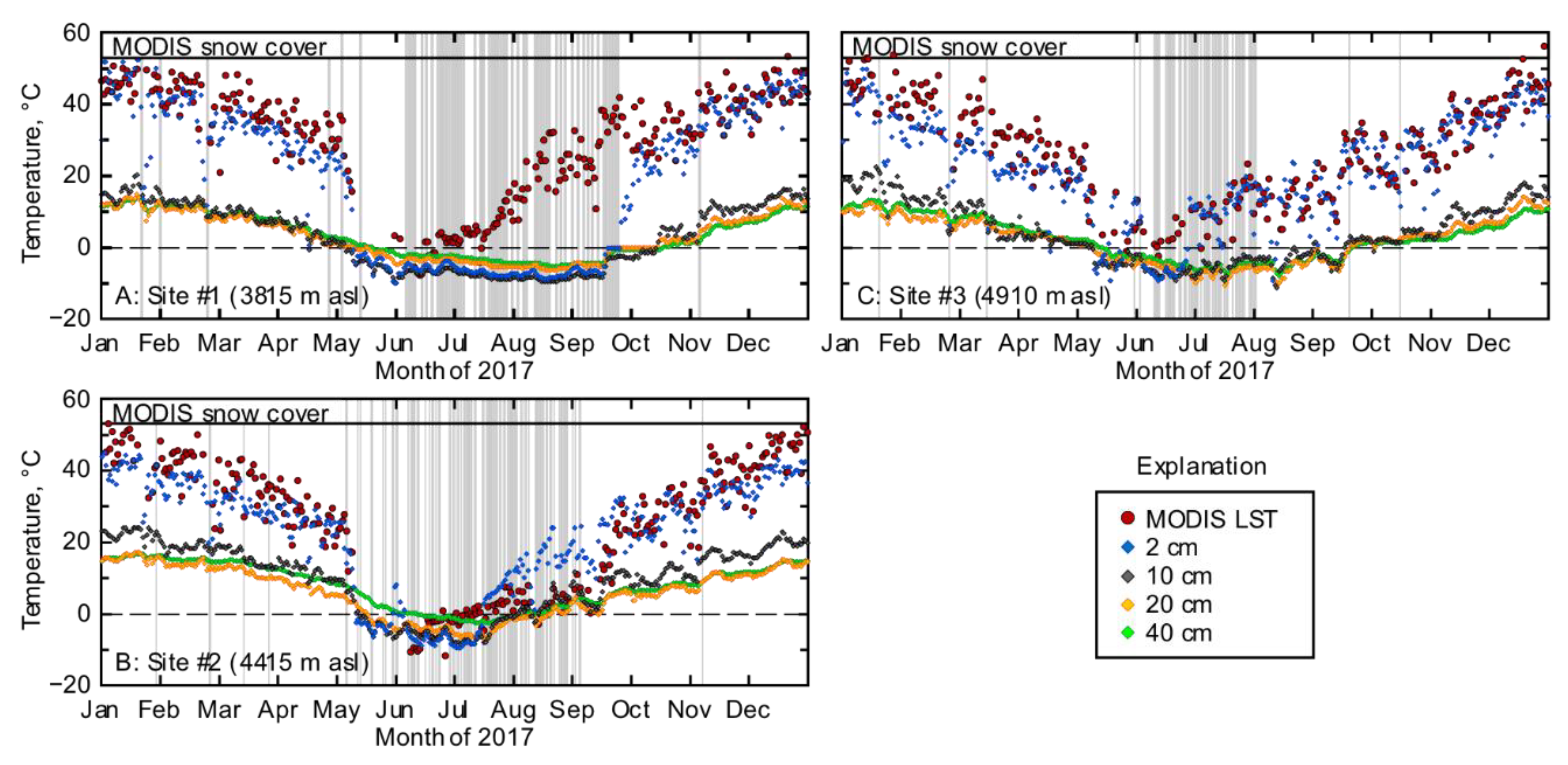
3.1. The Zero Curtain in the LST Data

The LST for the ~2 PM MODIS overflight of Ojos del Salado during the thawing season of 2017 is shown for Site #2 in Figure 3. The plateau near 0 °C between June 20 and July 14 is the zero curtain. 2 PM is near the peak of the diurnal temperature cycle, and thin ice films forming at night will likely not register then. The lack of LST records reflects the cloudy days.

MODIS LST images were consistently recorded for the three validation sites between 2003 and 2017. The seasonal temperature cycle is clearly visible in Figure 4, although the short zero curtains are not evident at this compressed temporal scale. The persistence of low winter temperatures was less at all three sites than the persistence of high summer temperatures. Gaps in the record are times when clouds obscured the ground. The maximum temperatures ranged among sites from ~50 °C at sites #1 and #2 to ~35 °C at Site #3. The minimum temperatures ranged much less, only rarely dipping below 0°C during the afternoon even at Site #3 (4910 m asl), 460 m above the altitude at permafrost was thought possible by Nagy et al. [16]. The LST at the lowest site, Site #1, consistently stayed above freezing for almost all years, consistent with the low probability of permafrost existence based on the surface mapping and numerical modeling of air temperatures [39,40,44]. The highest site, Site #3, near Barrancas Blancas shows consistent zero curtains during both freezing and thawing seasons.

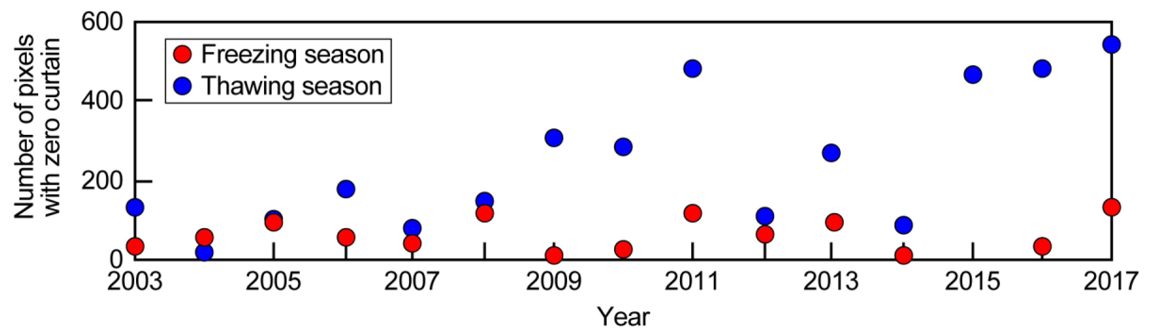
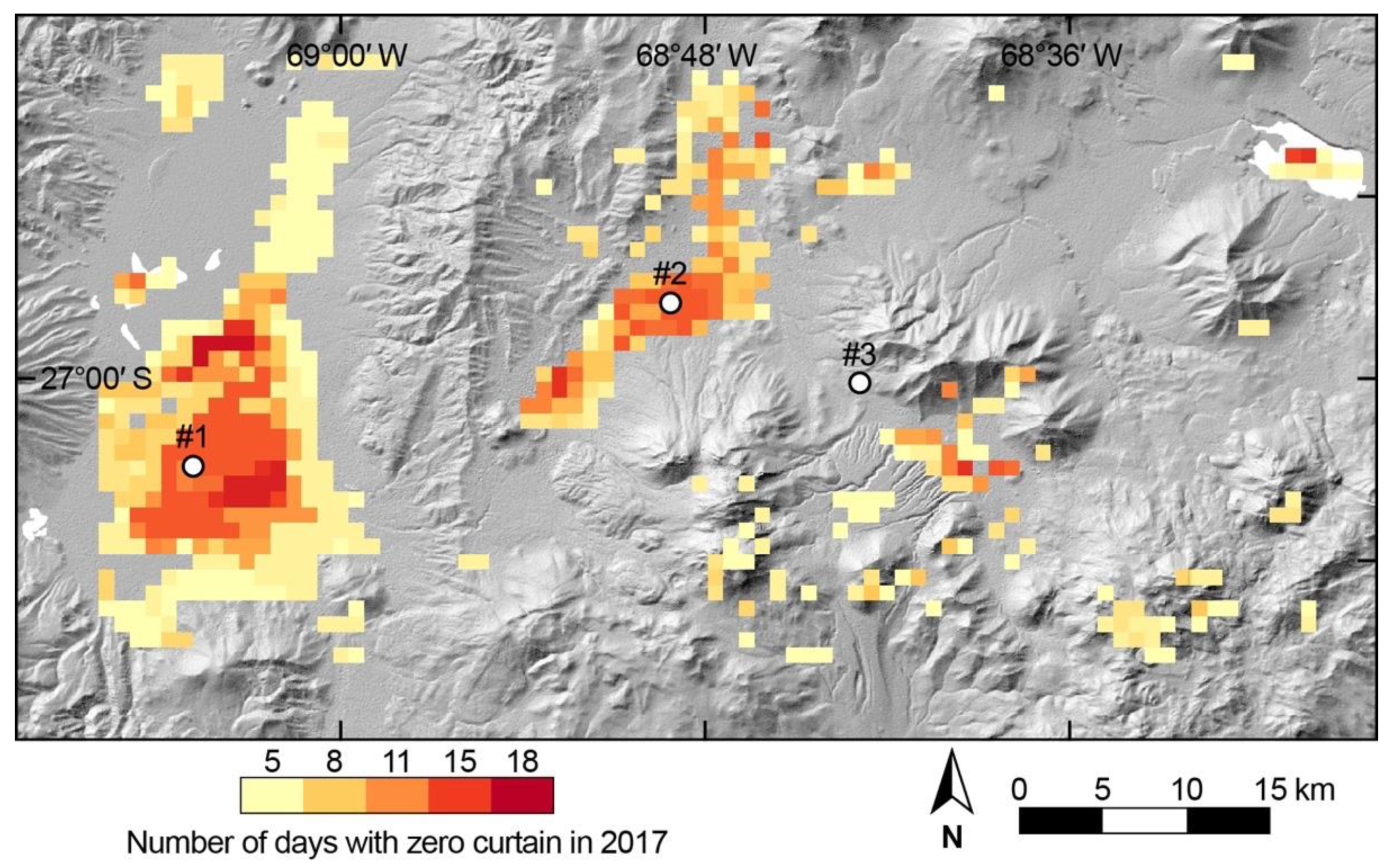
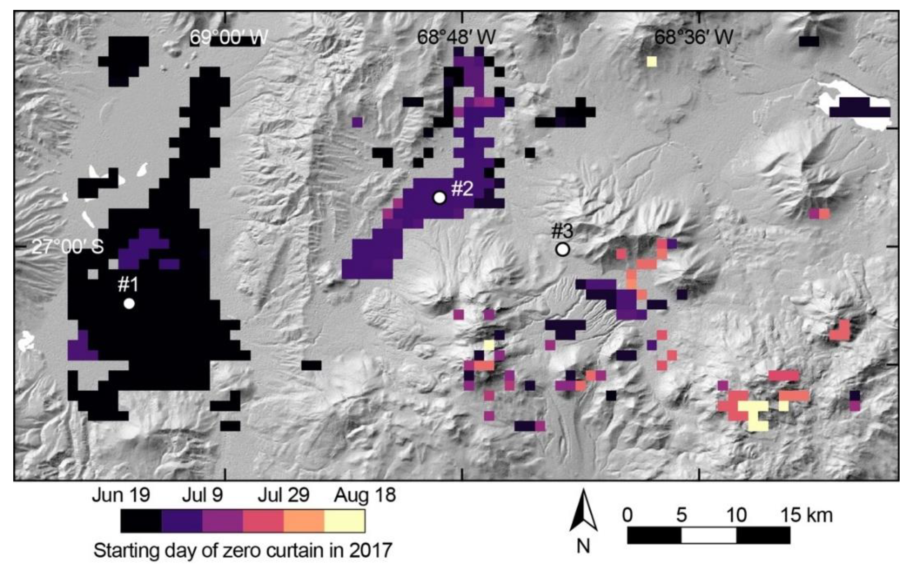
3.2. Occurrence of Zero Curtains in the Study Area

We analyzed 3393 pixels (87 × 39 km grid) with a 1-km spatial resolution in the study area for each of the 15 years (2003–2017). Approximately 60% of the study area is located above 4550 m asl, the altitude above which permafrost likely exists per Nagy et al. [16]. We produced two types of maps for thawing and freezing seasons of the years 2003–2017 using the Threshold Window algorithm: (a) Number of days with zero curtain (duration), and (b) starting date of the zero curtain. The number of pixels with detected zero curtains (Figure 5) shows significant differences between the thawing and freezing seasons. The area with zero curtains during the freezing season remained largely constant throughout the years. However, the area with zero curtain during the thaw has increased over the years. A notable exception was during 2015, where the number of pixels with zero curtain during the freezing season was anomalously high.

Zero curtains were observed in ~5% to 40% of areas above 4550 m asl between 2003 and 2017. In the majority of cases, the zero curtain was observed only during a single season. In each year, except 2015, less than 50 pixels showed zero curtains in both seasons. In other words, there was very little overlap between the areas with zero curtain detected only during freeze-up and the zero curtain detected only in the thaw (supplementary Figure S8). During the thaw, the zero curtain was detected largely in areas at low altitudes (e.g., Figure 6).

During freeze-up between 2003 and 2017, zero curtains were detected in late April to late May (supplementary Figure S9). In the higher altitude areas, the zero curtain started earlier than at lower altitudes, suggesting that the MODIS LST measurements reflect the temperature decrease with increasing altitude. During the thaw, zero curtains were detected between late June and early October. Zero curtains during the thaw of 2003–2010 were detected mostly in August. However, after 2010, zero curtains were detected earlier, during late June to the middle of July (e.g., Figure 7). These earlier starting dates during the thaw seasons may reflect the recent warming trends in the air temperatures over the Andes [45].

3.3. Comparison Between MODIS LST and In Situ Measured Ground Temperatures

The MODIS daytime LST is a measure of the ~2 PM skin temperature integrated over each 1 km² pixel. The skin temperatures are subject to short-term fluctuations caused by gusts of wind and the shadows of high-altitude clouds located over adjacent pixels. The km-scale skin temperature is weighted by the temperatures of the gravel of the pavements on the fans, whereas the subsurface temperature probes record the temperature of the soil beneath the pavement. Despite such different representations of ground temperatures, the measurements of daily MODIS LST and subsurface ground temperatures at the 2 cm depth in the three validation sites during 2017 agree well during the warm seasons (Figure 8), demonstrating the robustness of MODIS LST measurements for monitoring purposes. However, the correlation is less well established during the cold seasons. During 2017, the ground temperatures at the three validations sites were consistent at all depths (2–40 cm) during May–September, suggesting that the surface was covered with snow (see MODIS snow cover data, MYD10A1 [46], in Figure 8). Both MODIS snow cover data and the in situ measurements of ground temperatures at Site #3 show the fewest number of days with snow cover.

The MODIS LST at sites #1 and 2 show 15 days of sustained zero curtain during the thawing season of 2017. However, during this time at both sites, the subsurface temperatures measured at 2 cm were ~5–10 °C lower than the LST values. Only at Site #2 did the ground temperatures at the 40 cm depth show a persistent zero curtain, during which time the MODIS LST appear to agree (Figure 8B). We discuss in Section 4 below the complexities in the TIR remote sensing and their implications for the MODIS LST data.

4. Discussion

4.1. The MODIS LST Product

The basis for the detection of the zero curtain in this study is the MODIS LST product, of low (1 km) spatial but high (daily) temporal resolution. The MODIS LST is constructed from MODIS bands 31 and 32 (10.78–11.28 and 11.77–12.27 µm) using a split-window algorithm that corrects the data for atmospheric effects. Calculating LST from atmospherically corrected surface-emitted radiance is sensitive to the thermal emissivity: An error of 0.01 at 11 μm (MODIS band 31) corresponds to a temperature error of 0.6 K in the inversion of the Planck equation for the single wavelength. The default surface type (and emissivity in MODIS band 31) is soil (0.97: [47]). Although the MODIS LST algorithm assumes emissivity values for different surface types [48,49,50], only two are relevant in our validation sites on gravel pavements: Rock and snow (band 31: ε = 0.98). Coincidentally, the dacitic and volcanic pebbles composing the surfaces of the validation sites have the same emissivity at 11 μm used by the MODIS LST algorithm for soil. Therefore, the composition of the geological surface is unlikely to introduce temperature errors in the output images. MODIS snow-cover products (MOD10 and MYD10) are integrated into MODIS LST so that the calculation uses the proper emissivities, whether for the gravel surface or snow. Any discrepancy in LST due solely to the emissivities of the geologic surface and snow cover would be too small to detect readily in the time histories of LST for the three validation sites (Figure 4).

The cloud cover is detected and masked out in making the MODIS LST products [51] so that only the unobscured ground surface is represented. However, the lack of daily LST data during the seasonal thaw and freezing seasons may hinder the opportunities to detect the zero curtain occurrence. The percentage of data loss due to clouds over the study region from 2003 and 2017 ranged from ~20% to 60% in the mountainous areas. The percentage of data loss during March–September from 2003 to 2017 at the validation Site #1 ranged from 16% to 42% whereas at sites #2 and 3 it ranged from 27% to 56% (supplementary Table S6 and Figure S10).

The MODIS LST represents the dynamic balance between heating due to absorption of sunlight, diffusion of heat into the soil, and cooling due to emitted thermal-infrared radiance. The ‘true’ kinetic surface temperature, on the other hand, is susceptible to additional environmental changes, such as wind, evaporation, or condensation of water. These typically will make the LST more variable than the subsurface measurements, which are buffered by a large mass of adjacent soil. During the zero curtain times in 2017, the difference between the MODIS LST and the in situ ground temperatures at the 2 cm depth ranged between 1 and 6 °C at the validation sites (Figure 8). Considering the accuracy of the MODIS LST product of ~1 K [52] and the in situ ground temperatures, especially at the 2 cm depth, were comparable for much of the year. Exceptions to this rule evident in Figure 8 are discussed below.

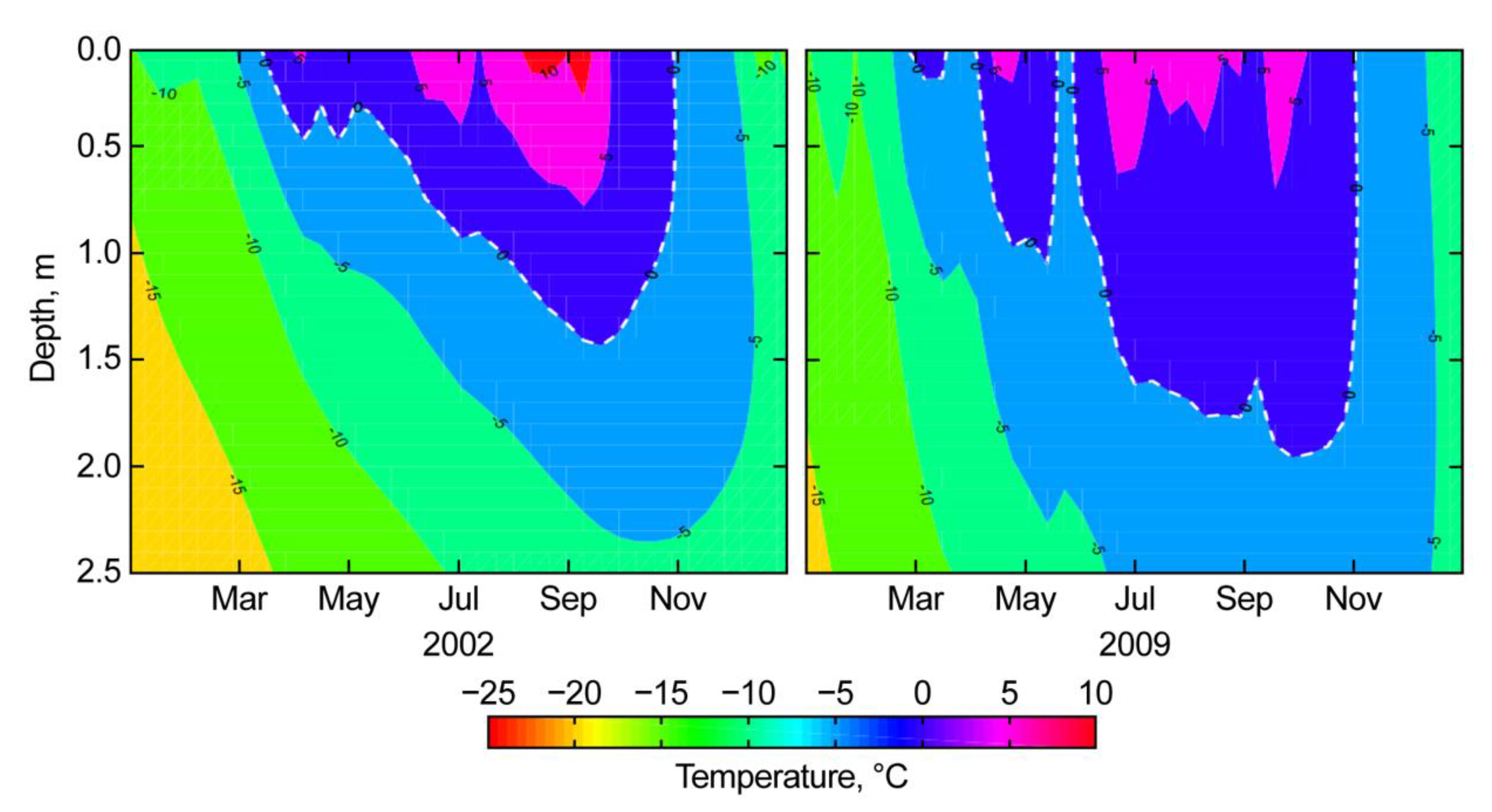
4.2. MODIS LST and Subsurface Temperature Profiles

Figure 8 compares the LST to the subsurface kinetic temperatures measured at the same time at the three validation sites. Although the LST and subsurface soil temperatures differ significantly depending on the type of vegetation covers (e.g., [22]), the surface at the validation sites remain barren most of the time (e.g., Table S2). As expected, the temperature at the 2 cm depth generally tracks the LST closely at all three sites, although it is lower by up to ~10 °C in summer. This may be due to the phase lag as the solar heating wave slowly penetrates the ground. In winter, the 2-cm temperature lowers to match the other subsurface values, but the afternoon LST rarely drops below zero.

Snow is highly reflective in the visible part of the spectrum (50–80%), yet 5% of the incoming solar energy is transmitted through cover 10–20 cm thick [53]. In contrast, snow absorbs efficiently in the thermal-infrared spectrum, such that the emitted radiation may originate only in the top 2 mm of the snow surfaces [54,55]. The nearly isothermal character of the subsurface as shown in Figure 8A is likely due to an insulating blanket of snow 10 cm or more in thickness, allowing the shallow subsurface to lose heat to deeper soil even as the snow surface is heated by the sun. In the limit, the LST of the snow cover could exceed the freezing point by at most a few °C, yet temperatures as high as 34 °C were recorded, even as the subsurface temperatures continued to decrease. This suggests that numerous large, sun-heated cobbles protruded from the thinning snowpack or that unresolved patches of snow-free ground had appeared but not over the subsurface sensors. By mid-October, the 2-cm temperature values have risen to match the LST, likely as the snow melted.

At Site #2 (Figure 8B) from mid-July until late September, the LST was lower than the temperature 2 cm down. The MODIS snow product indicates that there was snow cover during this time. This situation is the opposite of what occurred at the same season in Site #1. How could this happen, and what does it imply for the detection by MODIS of a zero curtain?

A likely explanation is that the snow cover was a thin veneer, thick enough so that the thermal infrared signal was radiated from its surface, unaffected by the ground beneath. On the other hand, the veneer was thin enough (i.e., <10–20 cm) that the ground was heated by irradiance from the sun at visible wavelengths. Thus, in mid-May, both the LST and the 2 cm temperature lowered to a few degrees below zero as the first snowfall was recorded.

During the time the ground was snow-covered or obscured by cloud, no meaningful zero curtain could be detected. This period included the likely freeze-up. By early June, the cloudiness cleared, and the surface of the snow rose from −10 °C to zero as the sun heated and thinned the snow cover. From mid-June to mid-July, the LST indicated a zero curtain. Thus, misleading zero curtains that pertain to thawing snow can be returned by the “Threshold Window” filtering algorithm.

At the high-altitude Site #3 (Figure 8C), subsurface zero curtains (10, 20, and 40 cm depth) occurred during both thaw (early May) and freeze-up (early October), but none occurred at the 2 cm depth or at the surface, both of which were 20 °C or warmer. Furthermore, except for the temperatures at 2 cm, the subsurface sites had similar temperatures throughout the winter, between the zero curtains. MODIS reported no snow cover before June or after August, so that snow has no role in explaining these relationships then. During the winter, however, on individual days, temperatures at both 2 cm and the immediate surface dropped ~12 °C to near zero, an occurrence likely associated with ephemeral snow cover. During the summer, temperatures at 20 and 40 cm remained close to each other while temperatures at 10 cm rose to intermediate values between the temperatures at the deeper sensors and the 2 cm depth. These observations likely resulted from solar warming of the surface. At Site #3, there was sufficient soil moisture to allow zero curtains at depth, but the circumstances precluded any at the surface.

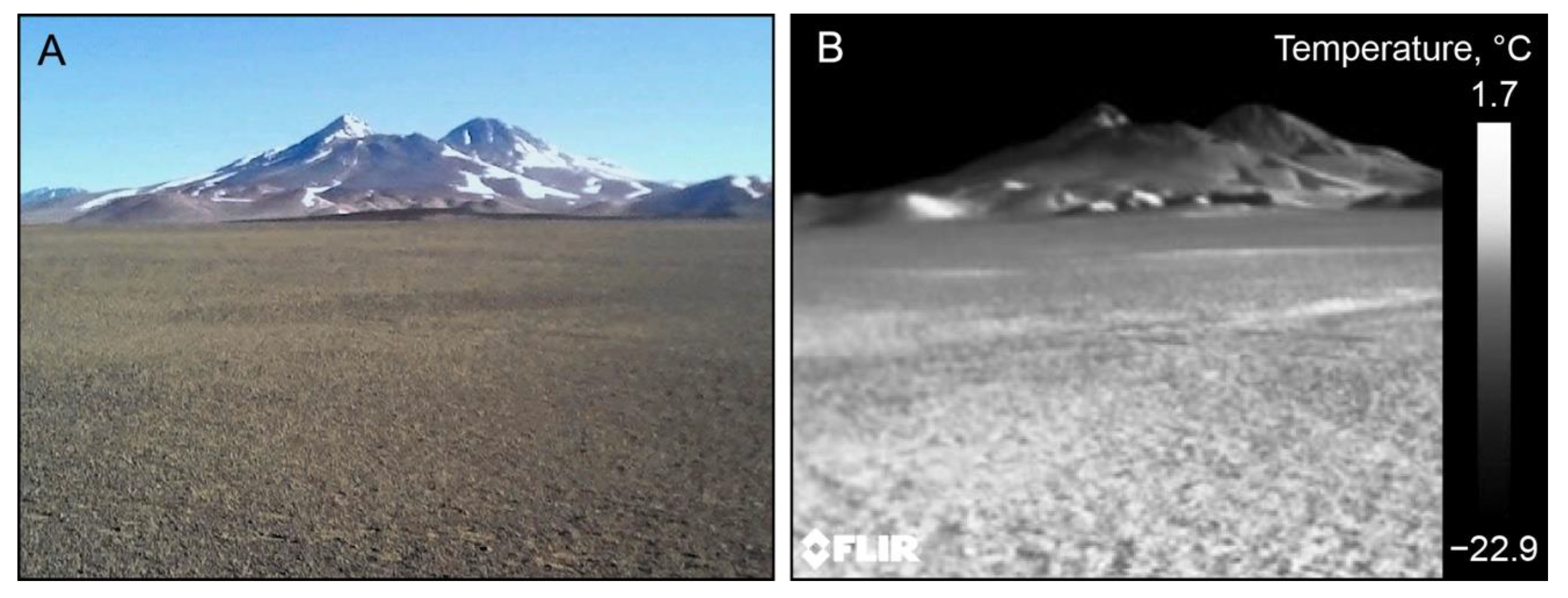
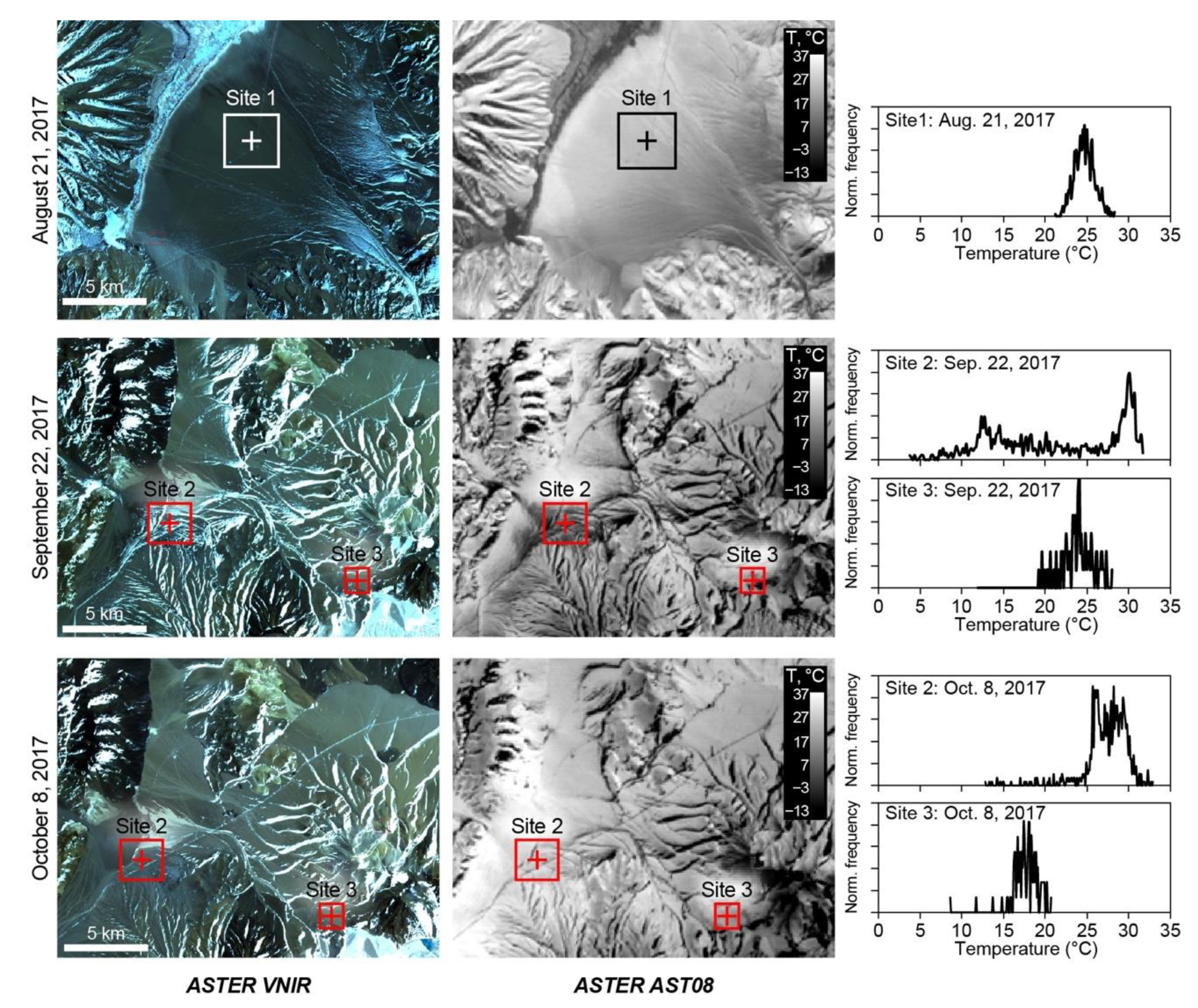
4.3. Effects of Scene Roughness

The alluvial fan surfaces at the validation sites were compositionally homogeneous and flat on a coarse km scale. However, we noticed that local fine-scale topography was variable, ranging from dry channels to small periglacial patterned grounds (supplementary Figures S1–S5). The manifestation of topographical variation in the emitted radiance at the thermal infrared spectrum can be seen in Figure 9, where subtle topographic features not discernible in the photograph can be resolved as bright pixels in the FLIR image. Inclusion of these features in low-resolution pixels causes the histogram of temperatures within those pixels to broaden. For example, the standard deviations within pixel aggregations simulating lower-resolution data in the plain in Figure 9 range from about 0.2 K at 2 m pixel⁻¹ to 2.5 K at 380 m pixel⁻¹. Topographic effects influencing the effective surface temperatures at the ASTER or MODIS scales are not large enough to affect the analysis in this study significantly. However, during the thaw, the radiance from unresolved patches of snow will mix with that from adjacent bare soil to lower the effective daytime LST.

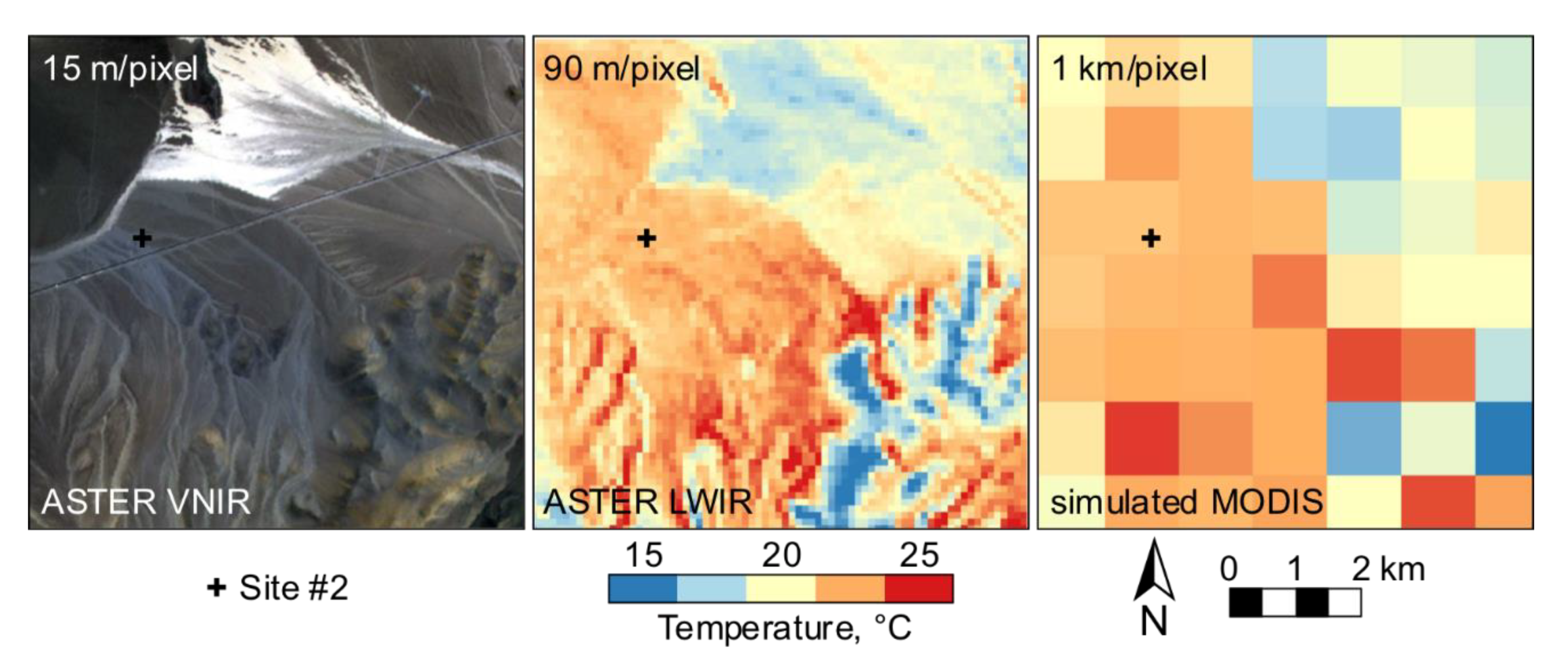
4.4. Spatial Resolution and Radiance Mixing

Although the validation sites appear to be homogeneous from the standpoint of the MODIS LST data, analysis of zero curtains elsewhere will encounter more complex surfaces and in any case there may be seasonal patches of snow unresolved by MODIS. ASTER, at 90 m pixel⁻¹, will produce more unmixed (“pure”) pixels in complex terrain, and thus will produce more pixels in which reliable assessments of the zero curtain can be made (Figure 10). Small seasonal snow patches provide one example, important in this study, of temperature mixing that may be reduced with improved resolution.

For this study, the temperature window in the Threshold Window filtering algorithm was set at ±3.5 °C to account for the MODIS LST accuracy of ~1 °C (1 σ), any variations in emissivity of different types of rocks, and effects of local topographic features that cannot be resolved at the spatial resolution of MODIS LST data. Many but not all mixed pixels of soil and snow will be filtered out with this setting.

Adjusting the size of the Threshold Window decreases or increases the number of data points to be counted as part of a zero curtain, decreasing or increasing false negatives or false positives, but a better approach might be to reduce the pixel size. For example, horizontal changes in the extent of permafrost in Tibet Plateau can be estimated to ~460–920 m in 30 years after accounting for the maximum vertical change of permafrost base during the same period (80 m [56,57]) and the average slope of the interior of the plateau (~5–10° [58]). The threshold window algorithm cannot capture changes at such a 100 m scale due to the relatively low resolution of the MODIS LST data. This limitation might be overcome by using ASTER data, with its higher spatial resolution than MODIS, but repeat acquisitions of ASTER images are too infrequent. A compromise may be possible with data fusion: Surface compositions can be mapped using the 15-m pixel−1 visible and 30-m pixel−1 near-infrared data while variations in the surface emissivity can be resolved from the 90-m pixel−1 ASTER products (Figure 11). With this information and the daily LST, it may be possible to generate the higher 90-m spatial resolution of the ASTER surface temperature product using the STARFM algorithm [59]. Data fusion might also be used with the high spatial but irregular and temporal resolution data of ECOSTRESS (

Table 2. Comparison of thermal-infrared sensors.

Sensor	Resolution		Launch Date
	Spatial	Temporal
GOES	Low (4 km)	High (3 h)	1981
AVHRR (NOAA)	Moderate (1 km)	High (daily)	1979
MODIS	Moderate (1 km)	High (daily)	2000
ASTER	High (90 m)	Low (16 days)	2000
Thematic Mapper	High (60 m)	Low (16 days)	1982
ECOSTRESS 1	High (38 × 69 m)	1 h of science data day−1	2019

¹ The ECOSTRESS products are in development and data are available only through “Early Adopters” program.

). However, to monitor subtle changes in permafrost extent in the future, we likely will need data with both high spatial and high temporal resolution.

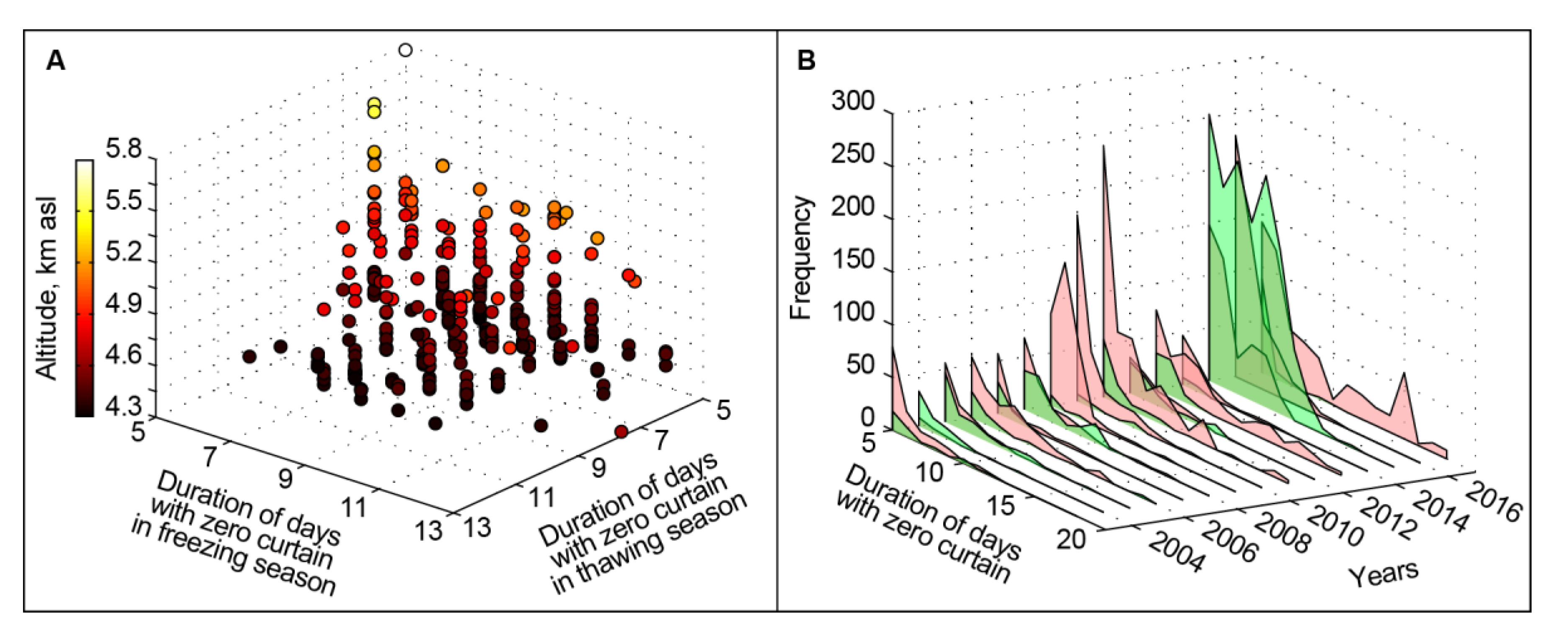
4.5. Seasonal Zero-Curtain Duration

Putkonen [12] stated that there is an asymmetry in the occurrence of the zero curtain during spring and autumn over permafrost, where the zero curtain appears during freeze-up, and over seasonally frozen ground, where the zero curtain appears during thaw. Figure 12 examines this asymmetry both as a correlation between the duration of freeze-up and thaw and as a function of altitude in the validation sites during 2015. Above ~5200 m asl, the zero-curtain duration of both freeze-up and thaw is about the same; at lower altitude, the duration of freeze-up exceeds the duration of thaw~40%.

Is the weak asymmetry revealed in Figure 12A due to a systematic trend, or is it the result of weather anomalies? In late March of 2015, before the general freeze-up, an extreme heat event occurred in central and northern Chile followed by an anomalously high precipitation event (>20 mm day⁻¹ [60]). Compared to other years, this extreme weather event must have supplied enough moisture to the soil to have resulted in the anomalously high number of pixels with zero curtains during both freeze-up and thaw that year (Figure 12A), so the anomaly did not increase any apparent asymmetry. During freeze-up, the zero curtain was detected in early April in high-altitude areas and in early June in low-altitude areas. The zero curtain during this time persisted for about two weeks. Later in the year, during the thaw, the zero curtain was detected only around early July with no contrast between the high- and low-altitude areas. The anomalously high precipitation from the March event may have been preserved in the soil over the winter and the increased soil moisture may have contributed to the sustained zero curtain during the thaw of 2015.

The weather anomaly aside, Figure 12B shows that the in the study area the maximum duration of the zero curtain during freeze-up, but not during thaw, may have increased erratically over the study period. The increase during freeze-up suggests that changes in the zero curtain can be detected on the decadal scale. The more constant and smaller number of zero curtain days during thaw indicates that the results are not random and that there has been little change. Taken together, the data plotted in Figure 12 suggest that there is little evidence at Ojos del Salado for the strong asymmetry predicted by Putkonen [12] for the zero-curtain freeze-up/thaw duration over permafrost. It may be that summer, but not winter, precipitation has been increasing in recent years but is not sufficient to carry over to the thaw. In all, these results are encouraging for the use of the zero curtain in climate-change studies.

4.6. Potential for Quantified Mapping of Seasonally Frozen Ground and Permafrost

The occurrence of the zero curtain requires moisture in the soil and low temperatures. Therefore, the identification of a zero curtain is a useful indicator of ice-rich frozen ground and possibly permafrost. We identify the following four parameters for the zero curtain that can be quantified using the Threshold Window algorithm: (a) Starting date, (b) duration, (c) seasonality, and (d) persistence over more than two seasons. The changes in the starting date of a zero curtain over time may indicate changes in the thermal regime of the soil due to changing environmental and climate conditions. According to Putkonen [12], the thermal regime in the soil would be different depending on the existence of permafrost underneath, and the asymmetric seasonality of the zero curtain may indicate whether it is due to seasonally frozen ground or the possible existence of permafrost. The intensity of freezing or thawing may dictate the duration of zero curtain, the changes of which can be mapped over time. On the basis of these parameters and the criteria for classifications of permafrost conditions (e.g., [61]), it is possible that a quantitative map of permafrost extent and the depth of the active layer can be estimated.

The probabilistic horizontal extent of permafrost based on the empirical relationship between ground temperature and mean annual air temperature has been mapped (e.g., [40]). The detection of permafrost using the Threshold Window algorithm, therefore, can validated using the probabilistic maps of permafrost produced from climate and geomorphological data. Further, the depth of the active layer can be estimated by numerically modeling heat diffusion into the ground using surface temperatures estimated from ASTER or MODIS data as constraints. For example, a heat-transfer model of soils that accounts for different estimates of moisture content [62,63] was run using MODIS LST (8-day mean) as an initial condition and used to numerically construct the thermal profiles of soils in a well-known permafrost region of Tibet (Figure 13; [64]). The ground temperatures calculated at various depths over time allowed the depth to the zero isotherm to be estimated for 2002 and 2009, consistent with the depths to the base of the active layer measured in the field [65]. Figure 13 shows that the depth of the zero isotherm decreased about 20 cm over the 7-year period. The model suggests that there was an extended period when −5 °C < LST <5 °C that may have been a zero curtain (intersection of the dark blue color and the top of the plot) in April–May 2002, and that it was shorter in 2009. Similarly, a zero curtain was predicted for October, and it too was shorter in 2009. Thus, this model suggests that there may have been a zero curtain not just at freeze-up but also during the spring thaw, inconsistent with Putkonen [12] (Figure 4). Further testing of the model will be necessary to resolve this issue.

5. Summary and Conclusions

We proposed a new approach to detect the occurrence of the zero curtain in land-surface temperature images, maintenance of the temperature at or near 0 °C due to the release of latent heat from freezing or thawing moisture in the soil. We used a “Threshold Window” filtering algorithm to analyze daily MODIS land surface temperature (LST) data over a cold region of the Atacama Andes in Chile, where periglacial features have been documented. Our results demonstrated that the zero curtain could be consistently identified in the MODIS data. This demonstration opens the path to identifying ice-rich permafrost using time series of LST images.

The duration, seasonality, and the starting time of the zero curtain for each year between 2003 and 2017 were mapped. We measured subsurface ground temperatures at depths of 2–40 cm at three validation sites located at altitudes of 3815, 4415, and 4910 m asl in 2017. The in situ observations of subsurface temperatures complemented the MODIS LST records and showed that, with exceptions during the spring, the LST agreed within a few degrees with temperature at the 2 cm depth. The subsurface temperature records showed clearly the presence of the zero curtain at depth, out of phase with the zero curtain at the surface, and illustrated the effects of thinning snow cover on the recovered zero curtain. Over the period of the study, the duration of the zero curtain during the thaw and freeze-up seasons appeared to fluctuate, consistent with what might be expected from annual changes in weather conditions. However, on Ojos del Salado, the zero curtains at freeze-up tended to be longer than those at thaw, and also may have shown a tendency to lengthen over the study period. We did not find convincing evidence of permafrost in our data or in the field, although there was local evidence of segregation ice.

Our test sites were chosen to minimize vegetation cover that would interfere with satellite measurement of the land-surface temperature, but in practical applications, vegetation cover and snow may hinder the availability of remotely sensed LST for this approach. Small-scale variations in surface composition and topographic conditions create different thermal components that are integrated over large areas for products with moderate spatial resolution, such as MODIS LST. Thermal-infrared sensors with higher spatial resolution, such as ASTER and ECOSTRESS, can be used to resolve the 100-m-scale horizontal changes in the extent of seasonally frozen ground and permafrost. Numerical modeling of the thermal regime of the ground using these surface temperature records may be useful to estimate the depth of thaw in ice-rich frozen grounds and permafrost.

References

1. Schuur, E.A.G.; McGuire, A.D.; Schadel, C.; Grosse, G.; Harden, J.W.; Hayes, D.J.; Hugelius, G.; Koven, C.D.; Kuhry, P.; Lawrence, D.M.; et al. Climate change and the permafrost carbon feedback. Nature 2015, 520, 171–179. [Google Scholar] [CrossRef]
2. Biskaborn, B.K.; Smith, S.L.; Noetzli, J.; Matthes, H.; Vieira, G.; Streletskiy, D.A.; Schoeneich, P.; Romanovsky, V.E.; Lewkowicz, A.G.; Abramov, A.; et al. Permafrost is warming at a global scale. Nat. Commun. 2019, 10, 264. [Google Scholar] [CrossRef] [Green Version]
3. French, H.M. The Periglacial Environment, 3rd ed.; John Wiley & Sons: Chichester, UK, 2007. [Google Scholar]
4. Smith, S.; Brown, J. Assessment of the Status of the Development of Standards for the Terrestrial Essential Climate Variables—T7—Permafrost and Seasonally Frozen Ground; Global Terrestrial Observing System: Rome, Italy, 2009.
5. Obu, J.; Westermann, S.; Bartsch, A.; Berdnikov, N.; Christiansen, H.H.; Dashtseren, A.; Delaloye, R.; Elberling, B.; Etzelmüller, B.; Kholodov, A.; et al. Northern Hemisphere permafrost map based on TTOP modelling for 2000–2016 at 1 km2 scale. Earth-Sci. Rev. 2019, 193, 299–316. [Google Scholar] [CrossRef]
6. Dobiński, W. Northern Hemisphere permafrost extent: Drylands, glaciers and sea floor. Comment to the paper: Obu, J.; et al. 2019. Northern Hemisphere permafrost map based on TTOP modeling for 2000–2016 at 1 km2 scale. Earth-Sci. Rev. 2019, 193, 103037. [Google Scholar] [CrossRef]
7. Turetsky, M.R.; Abbott, B.W.; Jones, M.C.; Anthony, K.W.; Olefeldt, D.; Schuur, E.A.G.; Koven, C.; McGuire, A.D.; Grosse, G.; Kuhry, P.; et al. Permafrost collapse is accelerating carbon release. Nature 2019, 569, 32–34. [Google Scholar] [CrossRef] [Green Version]
8. He, H.; Dyck, M. Application of Multiphase Dielectric Mixing Models for Understanding the Effective Dielectric Permitivity of Frozen Soils. Vadose Zone J. 2013, 12. [Google Scholar] [CrossRef]
9. Duncan, B.N.; Ott, L.E.; Abshire, J.B.; Brucker, L.; Carroll, M.L.; Carton, J.; Comiso, J.C.; Dinnat, E.P.; Forbes, B.C.; Gonsamo, A.; et al. Space-Based Observations for Understanding Changes in the Arctic-Boreal Zone. Rev. Geophys. 2020, 58, e2019RG000652. [Google Scholar] [CrossRef]
10. Du, J.; Watts, J.D.; Jiang, L.; Lu, H.; Cheng, X.; Duguay, C.; Farina, M.; Qiu, Y.; Kim, Y.; Kimball, J.S.; et al. Remote Sensing of Environmental Changes in Cold Regions: Methods, Achievements and Challenges. Remote Sens. 2019, 11, 1952. [Google Scholar] [CrossRef] [Green Version]
11. Outcalt, S.I.; Nelson, F.E.; Hinkel, K.M. The zero-curtain effect: Heat and mass transfer across an isothermal region in freezing soil. Water Resour. Res. 1990, 26, 1509–1516. [Google Scholar]
12. Putkonen, J. What dictates the occurrence of zero curtain effect? In Ninth International Conference on Permafrost; Kane, D.L., Hinkel, K.M., Eds.; Institute of Northern Engineering, University of Alaska Fairbanks: Fairbanks, AK, USA, 2008; pp. 1451–1455. [Google Scholar]
13. Yi, Y.; Kimball, J.S.; Chen, R.H.; Moghaddam, M.; Reichle, R.H.; Mishra, U.; Zona, D.; Oechel, W.C. Mapping permafrost landscape features using object-based image classification of multi-temporal SAR images. Cryosphere 2018, 12, 145–161. [Google Scholar] [CrossRef] [Green Version]
14. De Pablo, M.A.; Ramos, M.; Molina, A. Thermal characterization of the active layer at the Limnopolar Lake CALM-S site on Byers Peninsula (Livingston Island), Antarctica. Solid Earth 2014, 5, 721–739. [Google Scholar] [CrossRef] [Green Version]
15. Trombotto Liaudat, D. Geocryology of southern South America. In Late Cenozoic of Patagonia and Tierra del Fuego; Developments in Quaternary Sciences; Rabassa, J., Ed.; Elsevier: Amsterdam, The Netherlands, 2008; Volume 11, pp. 255–268. [Google Scholar]
16. Nagy, B.; Ignéczi, A.; Kovács, J.; Szalai, Z.; Mari, L. Shallow ground temperature measurements on the highest volcano on Earth, Mt. Ojos del Salado, Arid Andes, Chile. Permafr. Periglac. 2019, 30, 3–18. [Google Scholar] [CrossRef] [Green Version]
17. Baldis, C.T.; Trombotto Liaudat, D. Rockslides and rock avalanches in the Central Andes of Argentina and their possible association with permafrost degradation. Permafr. Periglac. 2019, 30, 300–304. [Google Scholar]
18. Obu, J.; Westermann, S.; Kääb, A.; Bartsch, A. Ground Temperature Map, 2000–2016, Andes, New Zealand and East African Plateau Permafrost; PANGAEA: Oslo, Norway, 2019. [Google Scholar]
19. French, H. Recent Contributions to the Study of Past Permafrost. Permafr. Periglac. 2008, 19, 179–194. [Google Scholar] [CrossRef]
20. Nitze, I.; Grosse, G.; Jones, B.M.; Romanovsky, V.E.; Boike, J. Remote sensing quantifies widespread abundance of permafrost region disturbances across the Arctic and Subarctic. Nat. Commun. 2018, 9, 5423. [Google Scholar] [CrossRef]
21. Kumar, S.V.; Dirmeyer, P.A.; Peters-Lidard, C.D.; Bindlish, R.; Bolten, J. Information theoretic evaluation of satellite soil moisture retrievals. Remote Sens. Environ. 2018, 204, 392–400. [Google Scholar] [CrossRef] [Green Version]
22. Prakash, S.; Norouzi, H.; Azarderakhsh, M.; Blake, R.; Khanbilvardi, R. Potential of satellite-based land emissivity estimates for the detection of high-latitude freeze and thaw states. Geophys. Res. Lett. 2017, 44, 2336–2342. [Google Scholar] [CrossRef] [Green Version]
23. Kim, Y.; Kimball, J.; Glassy, J.; McDonald, K. MEaSUREs Northern Hemisphere Polar EASE-Grid 2.0 Daily 6 km Land Freeze/Thaw Status from AMSR-E and AMSR2, Version 1; National Snow and Ice Data Center: Boulder, CO, USA, 2018. [Google Scholar]
24. Liu, L.; Schaefer, K.; Zhang, T.; Wahr, J. Estimating 1992–2000 average active layer thickness on the Alaskan North Slope from remotely sensed surface subsidence. J. Geophys. Res. 2012, 117, F01005. [Google Scholar] [CrossRef]
25. Wang, L.; Marzahn, P.; Bernier, M.; Ludwig, R. Mapping permafrost landscape features using object-based image classification of multi-temporal SAR images. ISPRS J. Photogramm. 2018, 141, 10–29. [Google Scholar] [CrossRef]
26. Chen, R.H.; Tabatabaeenejad, A.; Moghaddam, M. Retrieval of permafrost active layer properties using time-series P-band radar observations. IEEE T. Geosci. Remote 2019, 57, 6037–6054. [Google Scholar] [CrossRef]
27. Westermann, S.; Langer, M.; Boike, J.; Heikenfeld, M.; Peter, M.; Etzelmüller, B.; Krinner, G. Simulating the thermal regime and thaw processes of ice-rich permafrost ground with the land-surface model CryoGrid 3. Geosci. Model Dev. 2016, 9, 523–546. [Google Scholar] [CrossRef] [Green Version]
28. Aalto, J.; Karjalainen, O.; Hjort, J.; Luoto, M. Statistical Forecasting of Current and Future Circum-Arctic Ground Temperatures and Active Layer Thickness. Geophys. Res. Lett. 2018, 45, 4889–4898. [Google Scholar] [CrossRef] [Green Version]
29. Tao, J.; Koster, R.D.; Reichle, R.H.; Forman, B.A.; Xue, Y.; Chen, R.H.; Moghaddam, M. Permafrost variability over the Northern Hemisphere based on the MERRA-2 reanalysis. Cryosphere 2019, 13, 2087–2110. [Google Scholar] [CrossRef] [Green Version]
30. Wan, Z.; Hook, S.; Hulley, G. MOD11A1 MODIS/Terra Land Surface Temperature/Emissivity Daily L3 Global 1km SIN Grid V006, Distributed by NASA EOSDIS Land Processes DAAC. 2015. Available online: https://doi.org/10.5067/MODIS/MOD11A1.006 (accessed on 15 April 2018).
31. Wan, Z.; Hook, S.; Hulley, G. MYD11A1 MODIS/Aqua Land Surface Temperature/Emissivity Daily L3 Global 1km SIN Grid V006, Distributed by NASA EOSDIS Land Processes DAAC. 2015. Available online: https://doi.org/10.5067/MODIS/MYD11A1.006 (accessed on 15 April 2018).
32. Brown, O.B.; Minnett, P.J. MODIS Infrared Sea Surface Temperature Algorithm; Algorithm Theoretical Basis Document, NASA Contract Number NAS5-31361; University of Florida: Miami, FL, USA, 1994. [Google Scholar]
33. Hulley, G.C.; Hughes, T.; Hook, S.J. Quantifying uncertainties in land surface temperature (LST) and emissivity retrievals from ASTER and MODIS thermal infrared data. J. Geophys. Res. 2012, 117, D23113. [Google Scholar] [CrossRef] [Green Version]
34. NASA/METI/AIST/Japan Spacesystems, and U.S./Japan ASTER Science Team. ASTER Level 2 Surface Temperature Product, ASTER Kinetic Surface Temperature (AST_08), and Registered Radiance (AST_L1B version 3) Images from April 8, 2017 (Granule UR AST_L1B.003:2248631617), NASA EOSDIS Land Processes DAAC at the USGS Earth Resources Observation and Science (EROS) Center, Sioux Falls, South Dakota. Available online: https://doi.org/10.5067/ASTER/AST_08.003 (accessed on 1 October 2019).
35. Fan, Y.; Van Den Dool, H. A global monthly land surface air temperature analysis for 1948–present. J. Geophys. Res. 2008, 113, D01103. [Google Scholar] [CrossRef]
36. NASA JPL. NASA Shuttle Radar Topography Mission Global 1 arc Second, Distributed by NASA EOSDIS Land Processes DAAC at the USGS Earth Resources Observation and Science (EROS) Center, Sioux Falls, South Dakota. 2013. Available online: https://doi.org/10.5067/MEaSUREs/SRTM/SRTMGL1N.003 (accessed on 1 October 2019).
37. Kalnay, E.; Kanamitsu, M.; Kistler, R.; Collins, W.; Deaven, D.; Derber, J.; Gandin, L.; Saha, S.; White, G.; Woollen, J.; et al. The NCEP/NCAR 40-year re-analysis project. Bull. Am. Meteorol. Soc. 1995, 77, 437–471. [Google Scholar] [CrossRef] [Green Version]
38. Vargo, L.J.; Galewsky, J.; Rupper, S.; Ward, D.J. Sensitivity of glaciation in the arid subtropical Andes to changes in temperature, precipitation, and solar radiation. Glob. Planet. Chang. 2018, 163, 86–96. [Google Scholar] [CrossRef]
39. Trombotto, D.T. Survey of Cryogenic Processes, Periglacial Forms and Permafrost Conditions in South America; Revista do Instituto Geológico: São Paulo, Brazil, 2000; pp. 33–55. [Google Scholar]
40. Gruber, S. Derivation and analysis of a high-resolution estimate of global permafrost zonation. Cryosphere 2012, 6, 221–233. [Google Scholar] [CrossRef] [Green Version]
41. Baker, P.E.; Gonzalez-Ferran, O.; Rex, D.C. Geology and geochemistry of the Ojos del Salado volcanic region, Chile. J. Geol. Soc. 1987, 144, 85–96. [Google Scholar] [CrossRef]
42. Schneider, U.; Becker, A.; Finger, P.; Meyer-Christoffer, A.; Rudolf, B.; Ziese, M. GPCC Full Data Reanalysis Version 7.0: Monthly Land-surface Precipitation from Rain Gauges Built on GTS Based and Historic Data; Research Data Archive at the National Center for Atmospheric Research, Computational and Information Systems Laboratory. Available online: https://doi.org/10.5065/D6000072 (accessed on 10 January 2016).
43. Buchroithner, D.; Trombotto, D. Cryophenomena in the Cold Desert of Atacama. In EGU General Assembly Conference Abstracts; EGU: Vienna, Austria, 2012; Volume 14, p. 654. [Google Scholar]
44. García, A.; Ulloa, C.; Amigo, G.; Milana, J.P.; Medina, C. An inventory of cryospheric landforms in the arid diagonal of South America (high Central Andes, Atacama region, Chile). Quatern. Int. 2017, 438, 4–19. [Google Scholar] [CrossRef]
45. Falvey, M.; Garreaud, R.D. Regional cooling in a warming world: Recent temperature trends in the southeast Pacific and along the west coast of subtropical South America (1979–2006). J. Geophys. Res. 2009, 114, D04102. [Google Scholar] [CrossRef]
46. Hall, D.K.; Riggs, G.A.; Salomonson, V.V. MODIS/Terra Snow Cover 5-Min L2 Swath 500m. Version 5; NASA National Snow and Ice Data Center Distributed Active Archive Center: Boulder, CO, USA, 2006.
47. Baldridge, A.M.; Hook, S.J.; Grove, C.J.; Rivera, G. The ASTER spectral library version 2.0. Remote Sens. Environ. 2009, 113, 711–715. [Google Scholar] [CrossRef]
48. Snyder, W.C.; Wan, Z.; Zhang, Y.; Feng, Y.Z. Classification-based emissivity for land surface temperature measurement from space. Int. J. Remote Sens. 1998, 19, 2753–2774. [Google Scholar] [CrossRef]
49. Wan, Z. New refinements and validation of the MODIS land-surface temperature/emissivity products. Remote Sens. Environ. 2008, 112, 59–74. [Google Scholar] [CrossRef]
50. Wan, Z. New refinements and validation of the Collection-6 MODIS land-surface temperature/emissivity products. Remote Sens. Environ. 2014, 140, 36–45. [Google Scholar] [CrossRef]
51. Ackerman, S.A.; Frey, R. MODIS Atmosphere L2 Cloud Mask Product (35_L2). NASA MODIS Adaptive Processing System at the Goddard Space Flight Center, Greenbelt, MD, USA. 2015. Available online: http://dx.doi.org/10.5067/MODIS/MYD35_L2.006 (accessed on 10 December 2019).
52. Wan, Z.; Zhang, L.; Zhan, Q.; Li, Z.L. Quality assessment and validation of the MODIS global land surface temperature. Int. J. Remote Sens. 2004, 25, 261–274. [Google Scholar] [CrossRef]
53. Warren, S.G. Optical properties of ice and snow. Philos. T. Roy. Soc. A 2019, 377, 20180161. [Google Scholar] [CrossRef]
54. Brandt, R.E.; Warren, S.G. Solar-heating rates and temperature profiles in Antarctic snow and ice. J. Glaciol. 1993, 39, 99–110. [Google Scholar] [CrossRef] [Green Version]
55. Salisbury, J.W.; D’Aria, D.M.; Wald, A. Measurements of thermal infrared spectral reflectance of frost, snow, and ice. J. Geophys. Res. 1994, 99, 24235–24240. [Google Scholar] [CrossRef]
56. Cheng, G.; Wu, T. Responses of permafrost to climate change and their environmental significance, Qinghai-Tibet Plateau. J. Geophys. Res. Earth 2007, 112, F02S03. [Google Scholar] [CrossRef] [Green Version]
57. Changwei, X.; Gough, W.A.; Lin, Z.; Tonghua, W.; Wenhui, L. Temperature-dependent adjustments of the permafrost thermal profiles on the Qinghai-Tibet Plateau, China. Arct. Antarct. Alp. Res. 2015, 47, 719–728. [Google Scholar] [CrossRef] [Green Version]
58. Liu-Zeng, J.; Tapponnier, P.; Gaudemer, Y.; Ding, L. Quantifying landscape differences across the Tibetan plateau: Implications for topographic relief evolution. J. Geophys. Res-Earth 2008, 113, F04018. [Google Scholar] [CrossRef] [Green Version]
59. Gao, F.; Masek, J.; Schwaller, M.; Hall, F. On the blending of the Landsat and MODIS surface reflectance: Predict daily Landsat surface reflectance. IEEE Trans. Geosci. Remote. Sens. 2006, 44, 2207–2218. [Google Scholar]
60. Barrett, B.S.; Campos, D.A.; Vicencio Veloso, J.; Rondanelli, R. Extreme temperature and precipitation events in March 2015 in central and northern Chile. J. Geophys. Res. Atmos. 2016, 121, 4563–4580. [Google Scholar] [CrossRef] [Green Version]
61. Moore, J.P.; Ping, C.L. Classification of Permafrost Soils. Soil Horiz. 1989, 30, 98–104. [Google Scholar] [CrossRef] [Green Version]
62. Liu, L.; Sletten, R.S.; Hagedorn, B.; Hallet, B.; McKay, C.P.; Stone, J.O. An enhanced model of the contemporary and long-term (200 ka) sublimation of the massive subsurface ice in Beacon Valley, Antarctica. J. Geophys. Res. Earth Surf. 2015, 120, 1596–1610. [Google Scholar] [CrossRef]
63. Liu, L.; Sletten, R.S.; Hallet, B.; Waddington, E.D. Thermal regime and properties of soils and ice-rich permafrost in Beacon Valley, Antarctica. J. Geophys. Res. Earth 2018, 123, 1797–1810. [Google Scholar] [CrossRef]
64. Gillespie, A.R.; Batbaatar, J.; Sletten, R.S.; Trombotto, D.; O’Neal, M.; Hanson, B.; Mushkin, A. Monitoring and mapping soil ice/water phase transitions in arid regions. In Geological Society of America Abstracts with Programs; Geological Society of America: Boulder, CO, USA, 2017. [Google Scholar]
65. Zhao, L.; Wu, Q.; Marchenko, S.; Sharkhuu, N. Thermal state of permafrost and active layer in Central Asia during the International Polar Year. Permafr. Periglac. 2010, 21, 198–207. [Google Scholar] [CrossRef] [Green Version]
Figure 1. The zero curtain. (A) Daily ground temperatures (2 PM local) measured at various depths in the active layer above permafrost (location at 76.55414° N, 68.561680° W, 190 m asl) near Qaanaaq, Greenland. During 2015, there was a prominent zero-curtain effect due to the phase transition of water in the soil. During this time, the ground temperature was maintained at or near 0 °C at depths of 15 and 25 cm. Deeper than 30 cm the temperature never exceeded freezing, and near the immediate surface (not shown) the ground temperatures were commonly variable due to solar heating of the surface, complicating the effects of wind and cloudiness. This zero curtain was only observed from September to early October, during freeze-up, but not during the spring thaw. Unpublished data from R.S. Sletten. (B) Schematic from Putkonen [12] showing the modeled heat flow during freezing and thawing seasons. During freeze-up (red squares), the soil temperatures at the 0.5–1 m depth quickly reaches the freezing point, such that no heat diffusion upward (driven by the temperature gradient) can occur. The zero curtain will be maintained until all water in the active layer freezes. During the thaw (blue circles), the high thermal gradient in the soil ensures efficient heat flow and the soil will consistently warm with no zero curtain.
Remotesensing 12 00695 g001
Figure 2. Maps showing the study area and the mean annual air temperature for 2018. The numbered circles indicate the locations of validation sites where we measured subsurface ground temperatures. The Chilean customs office is marked with an symbol. The air temperatures were calculated from the GHCN CAMPS long-term (1981–2010) monthly mean dataset of air temperature (0.5° pixel−1 [35]) and were scaled to the resolution of SRTM DEM (30 m pixel−1) using the long-term (1981–2010) monthly mean NCEP/NCAR reanalysis dataset of lapse rate (2.5° pixel−1 [37]). The background hillshade image was constructed from 1 arcsec SRTM DEM (SRTMGL1).
Remotesensing 12 00695 g002
Figure 3. The LST time series for the thawing season, 2017, at Site #2. The zero-curtain (red data points) followed a protracted period of cloudiness during which there were no LST measurements of the ground surface.
Remotesensing 12 00695 g003
Figure 4. MODIS land surface temperatures at 2 PM (local) from 2003 to 2017 for the three validation sites.
Remotesensing 12 00695 g004
Figure 5. The number of pixels with zero curtain from 2003 to 2017. Out of the 3393 pixels analyzed for the study area (87 × 39 grid) the number of pixels with zero curtain during the thawing seasons have increased over time, while the values for the freezing seasons have remained approximately constant. Note the exception in 2015, for which the number of pixels with zero curtain during freeze-up was not plotted due to an anomalously high number of zero curtain pixels (1260).
Remotesensing 12 00695 g005
Figure 6. Number of days with zero curtains during the thaw season of 2017.
Remotesensing 12 00695 g006
Figure 7. The starting day of the zero curtain, determined using the Threshold Window algorithm, during the thaw season of 2017.
Remotesensing 12 00695 g007
Figure 8. Validation site temperatures at 2 PM. (A) Site #1. Between early June and mid-July, LSTs were near freezing and the 2 cm temperatures were about the same as at 10 cm, by late September increasing to 0 °C, later rising to match the LST. (B) Site #2. There was a late-June zero curtain in the LST. After the thaw, the LST was lower than the 2 cm temperature. (C) Site #3. Subsurface zero curtains, but none in the LST, occurred during both and freeze-up. The MODIS snow cover data is MYD10A1 [46].
Remotesensing 12 00695 g008
Figure 9. Validation Site #2 (26.9586° S and 68.8190° W, 4415 m asl) looking east over on a flat homogeneous alluviated plain. (A) View from the ground; (B) FLIR thermal-infrared image taken from the same spot and view angle. The images are about 6 km across at the foot of the mountain. The resolution of the FLIR image ranges from ~2 cm pixel−1 in the foreground to ~15 m pixel−1 at the foot of the mountain, ~12 km away.
Remotesensing 12 00695 g009
Figure 10. ASTER image pairs (VNIR and Surface Kinetic Temperature, AST08) for three dates in 2017. On 21 August, a 1-km2 MODIS pixel indicated Site #1 to be snow-covered, which the 15-m pixel−1 ASTER VNIR image disagrees with. On 22 September, MODIS indicated both sites #2 and #3 to be snow-free; ASTER shows them to be largely bare. On 8 October, MODIS indicates both sites #2 and #3 to be snow-free, which ASTER confirms. The MODIS snow classifications are binary (snow or no-snow). Modal temperatures (11:43 AM local AST08) for snow-free pixels are 23–30 °C and 12 °C for largely snow-covered pixels (22 September, SE corner Site #2). Even the lowest temperatures for snow cover or partial cover were above zero, implying significant temperature mixing with sun-heated rocks rising above the snow.
Remotesensing 12 00695 g010
Figure 11. Effect of resolution. The heterogeneity in topographic and geologic features visible from an ASTER 15-m VNIR image (left, AST_L1B_00304082017144319 (11:43 AM local): RGB = band 3 (0.81 μm), band 2 (0.66 μm), band 1 (0.56 μm)) are resolved less well in an ASTER 90-m Surface Kinetic Temperature product (middle, AST_08_00304082017144319) produced from TIR bands (RGB=band 13 (10.6 μm), band 11 (9.1 μm), band 10 (8.3 μm)). Validation Site #2 (marked with +) was chosen on an alluvial plain so that the variation of topography and surface composition under a single MODIS pixel is minimal. An image of the ASTER Surface Kinetic Temperature image resampled to the 1-km resolution of MODIS (left) shows significant mixing in high relief and compositionally varied sites (e.g., lower right part of the scene). Higher resolution is necessary for accurate estimations of LST.
Remotesensing 12 00695 g011
Figure 12. The zero-curtain duration for all pixels in which zero curtains were detected during both freeze-up and thaw. The zero curtain was only recognized for durations of five days or more. (A) Versus altitude (2015 only). Two-season zero curtains were not detected below 4300 m asl due to warm temperatures there. Above 5800 m asl, the ground was too cold for persistent thaws. At intermediate altitudes, there was sufficient soil moisture for both near-surface freezing and thawing. (B) Zero-curtain duration during freeze-up (red) and thaw (green) plotted against the corresponding years.
Remotesensing 12 00695 g012
Figure 13. The thermal profiles calculated using a heat-transfer model [62,63,64] for an ice-rich permafrost region in the Fenghuo Shan site (34.69°N and 92.89°E, 4938 m asl) in Tibet. The white dashed lines are the 0 °C isotherms that are used to determine the active-layer thickness. The modeled values are consistent with in-situ measured changes in active-layer thickness from 1.4 to 1.9 m between 2002 and 2009 [65].
Remotesensing 12 00695 g013