Quantifying Drought Sensitivity of Mediterranean Climate Vegetation to Recent Warming: A Case Study in Southern California

Abstract

A combination of drought and high temperatures (“global-change-type drought”) is projected to become increasingly common in Mediterranean climate regions. Recently, Southern California has experienced record-breaking high temperatures coupled with significant precipitation deficits, which provides opportunities to investigate the impacts of high temperatures on the drought sensitivity of Mediterranean climate vegetation. Responses of different vegetation types to drought are quantified using the Moderate Resolution Imaging Spectroradiometer (MODIS) data for the period 2000–2017. The contrasting responses of the vegetation types to drought are captured by the correlation and regression coefficients between Normalized Difference Vegetation Index (NDVI) anomalies and the Palmer Drought Severity Index (PDSI). A novel bootstrapping regression approach is used to decompose the relationships between the vegetation sensitivity (NDVI–PDSI regression slopes) and the principle climate factors (temperature and precipitation) associated with the drought. Significantly increased sensitivity to drought in warmer locations indicates the important role of temperature in exacerbating vulnerability; however, spatial precipitation variations do not demonstrate significant effects in modulating drought sensitivity. Based on annual NDVI response, chaparral is the most vulnerable community to warming, which will probably be severely affected by hotter droughts in the future. Drought sensitivity of coastal sage scrub (CSS) is also shown to be very responsive to warming in fall and winter. Grassland and developed land will likely be less affected by this warming. The sensitivity of the overall vegetation to temperature increases is particularly concerning, as it is the variable that has had the strongest secular trend in recent decades, which is expected to continue or strengthen in the future. Increased temperatures will probably alter vegetation distribution, as well as possibly increase annual grassland cover, and decrease the extent and ecological services provided by perennial woody Mediterranean climate ecosystems as well.

1. Introduction

Globally, CMIP5 climate models consistently project future warming and drying in most Mediterranean climate regions through the poleward-expanding subtropical subsidence [1,2,3]. Previous studies have suggested that the impacts of climate fluctuations on ecosystem processes become less predictable as climate extremes increase in frequency [4,5]. The resulting ecosystem changes can have many implications. As vegetation distributions change, so will habitat characteristics, potentially to the detriment of some species. Mediterranean climate regions are diversity hotspots, with large numbers of endemic and threatened species dependent upon specific habitat types [6]. Conversion of woody shrub cover to grasslands can lead to slope instability and increased landslides and erosion [7]. Winter and spring droughts in a Mediterranean climate zone could induce anomalies in ecosystem–atmosphere CO₂ fluxes and reduce both gross primary productivity (GPP) and ecosystem respiration significantly [8,9]. There has been increasing concern about a shift in Mediterranean climate ecosystems from “near-neutral” to a long-term carbon source, due to climate extremes or other disturbances in the near future [9,10,11].

California is a biodiversity hotspot and home to more species of plants and animals than any other state in the U.S. [12]. The mild temperatures and winter rain of the Mediterranean climate provides favorable conditions for such great species richness in the state [13]. Although the vegetation is drought-adapted, increasing aridity and drought intensity can be a threat to Mediterranean climate vegetation communities and potentially lead to land cover changes, such as the replacement of woody vegetation by grassland [14]. The recent exceptional California drought (from 2012–2016) was characterized by prolonged precipitation deficits, exacerbated by extremely warm temperatures and associated high rates of evapotranspiration [15]. This produced particularly large negative deviations in the Palmer Drought Severity Index (PDSI), and this drought may have been the most severe drought in the last 1200 years [15]. An analysis of the role of elevated temperatures associated with greenhouse gases in contributing to the severity of the drought concluded that there has been a significant imprint of anthropogenic climate change in producing drought [16]. The recent Californian drought cannot be viewed in isolation but, instead, as occurring in the context of a longer-term trajectory towards warmer and more arid conditions over the U.S. Southwest and Southern California over the past century [17,18,19,20]. Since entering the 21st century, Southern California has experienced three prolonged droughts (i.e., 2002–2003, 2007–2009, and 2012–2016). A prolonged drought is defined as a consecutive period of more than one year (12 months) with PDSI values ≤ −2.0 (moderate drought) [21]. The Californian droughts have been shown to be more and more severe and persistent. Thus, drought damage to the Californian Mediterranean ecosystems has been hypothesized to increase in the future. The 2012–2016 drought, occurring in the context of a multi-decadal trend of increasing temperature, can be seen as an example of the type of drought that will characterize the future. In addition to direct effects of drought, in terms of vegetation health and mortality, high temperatures and aridity produce increased pathogen impacts and fire danger [22,23].

According to NOAA’s climate change assessment [24], the annual temperature of the U.S. Southwest is projected to increase by 1.8–3.4 °C over the 2041–2070 period. However, over California, the global climate models (GCMs) have displayed poor consensus on future precipitation changes, with some models trending drier, and others wetter [25]. Moreover, it is still poorly understood whether a slight increase in precipitation, which is projected to occur in some areas of California, can offset the negative effects of the hotter droughts. Despite the uncertainty in precipitation, the potential impacts of “global-change-type drought” (simultaneous drought and heat waves; [26]) for vegetation health have been widely documented and cannot be ignored [27,28,29,30,31,32,33,34,35,36]. The co-occurrence of heat and drought events can impose considerable strains on plant functions [37]. For example, rising temperatures can increase carbohydrate consumption, reduce photosynthesis, and force greater stomatal closure [38].

The major vegetation types in the coastal zone of Southern California are chaparral, coastal sage scrub, grassland, and forest-woodland [39]. Not only do these vegetation types contain many endemic plant and animal species, but they also provide important ecosystem services to the people who live in the region [40]. These services include maintaining slope and soil stability, clean water resources, recreation, and visually attractive landscapes [41]. However, due to the appreciable rise of California’s population [42], significant areas of the natural land-covers in California have been converted to developed lands [43,44]. Although many Mediterranean climate plants are well adapted to short-term droughts, additional heat stress can significantly compound the effects of drought stress. Many species tend to close their stomata to reduce water loss in drought, which makes heat stress much more severe when transpirational cooling is reduced [37]. Furthermore, high temperatures may accelerate the demography of insect populations and exacerbate mortality during drought [45]. However, some evidence has been presented indicating reduced vulnerability of some vegetation communities to hotter drought [30]. For instance, warmer conditions may promote tree growth in cold regions [46]. Some species have developed compensatory physiological mechanisms to decrease the combined drought and heat stress; for example, reducing embolism by xylem refilling [47], down-regulation of respiration [48], and acclimation to recurrent droughts [49]. Furthermore, compared to natural vegetation communities, vegetation in developed lands (which may be continuously irrigated during drought) may be less affected by recent and future droughts and warming. Thus, understanding which vegetation communities are vulnerable to upcoming hotter droughts and which communities are resistant to them is crucial for climate change adaptation.

A coarse-scale analysis of the state-wide aridity and vegetation response to the 2012–2016 drought indicated that this drought was the most severe in the southern regions of California [17]. Moreover, [17] suggests that a hydroclimatic dipole has contributed to the stronger drying of Southern California than the north region. A detailed study of the impacts of the recent drought on the vegetation greenness of Southern California can thus provide insights into the relative sensitivities of different vegetation types or geographic sub-regions to prolonged warming and drying anticipated in the 21st century. These insights are important for developing environmental management policies for the future. A recent study by [50] revealed that the favorable soil water conditions of the deep-rooted chaparral makes them less sensitive to short-term drought events, but particularly vulnerable to prolonged droughts, as they are not adapted to soil water depletion, such as that which occurred in the 2012–2016 California drought. By contrast, the shallow-rooted coastal sage scrub (CSS) displayed a low sensitivity to the recent multi-year drought, indicating a better adaptation to persistent dry conditions [50]. The differential behavior of the two shrublands during drought is a result of long-term environmental adaption. However, as the local climate rapidly warms, it is of high significance to further investigate how these vegetation communities will respond to drought under both a warmer and drier climate. Additionally, as many forest trees can make use of deeper soil water and grass may recover quickly after intermittent rainfalls, we assume forest and grass are more resistant to the hotter droughts than chaparral and CSS. We further assume precipitation will slightly decrease in Southern California as the drought becomes more severe in the future, which may aggravate drought stress in these vegetation types.

In this study, to test the assumptions outlined above, we use a geospatially explicit comparative analysis of temporal trends in aridity and geographic patterns, as measured by the PDSI and NDVI response of Mediterranean chaparral, CSS, grassland, forest-woodland, and vegetation in developed lands, to assess the relative sensitivity of these vegetation types to increased warming and aridity. Following [51], we examine the regression slopes between NDVI and PDSI to measure vegetation sensitivity to drought. Here, sensitivity represents the likelihood of abnormal vegetation dynamics in a climate extreme. Previous studies have found strong linear relationships between NDVI and photosynthesis activities, carbon exchange, and moisture fluxes measured at towers [5,52,53]. Thus, remotely sensed continuous time-series of NDVI provides a consistent and repeatable measurement of vegetation condition, which is appropriate for capturing the effects of drought stress [54]. In addition, we also aim to identify the relative importance of temperature and precipitation in controlling the amplitude of extreme-drought impacts on Mediterranean climate vegetation. This can help strengthen our understanding of the possible ecosystem changes, given the expected future climate change scenario.

2. Materials and Methods

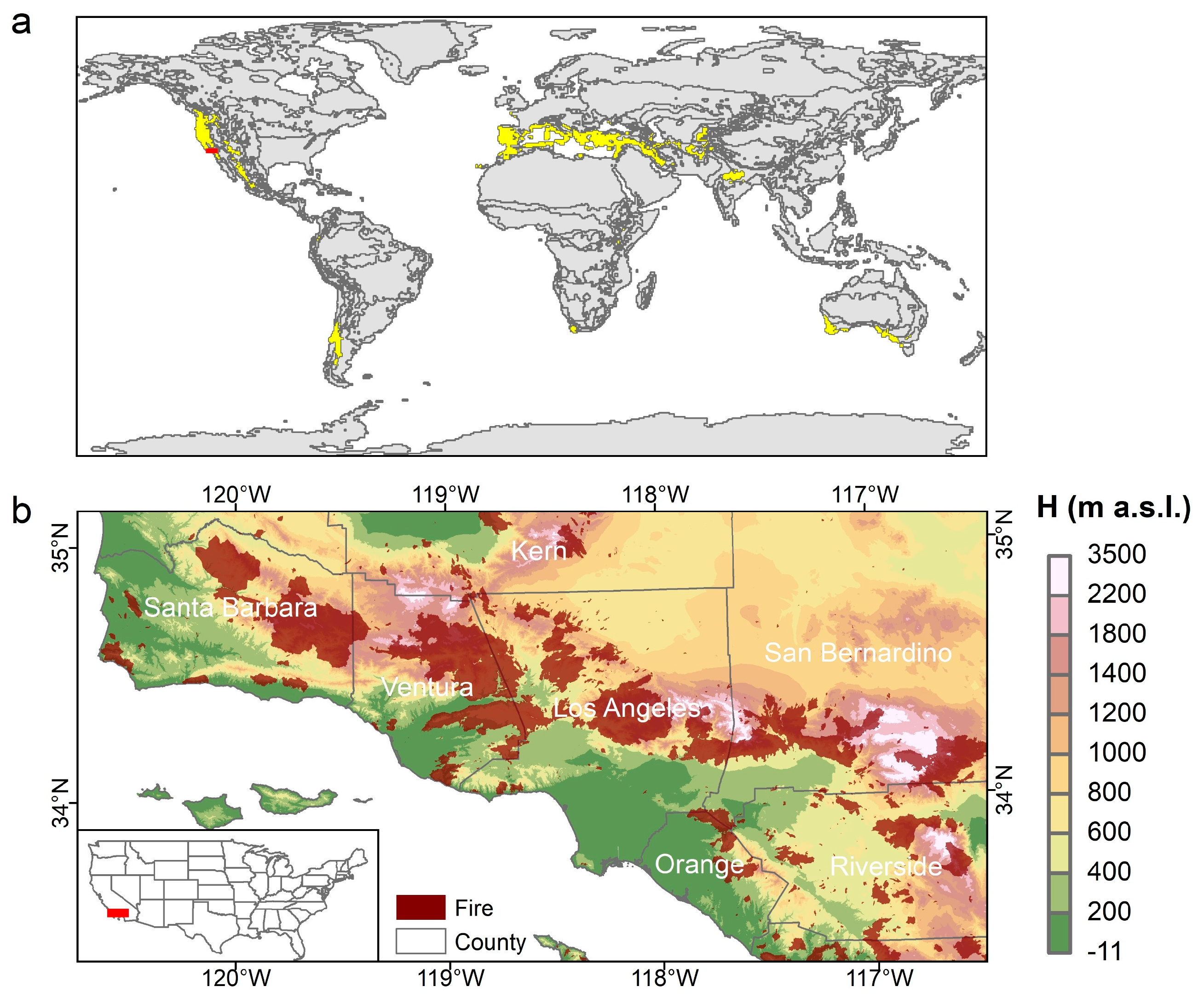
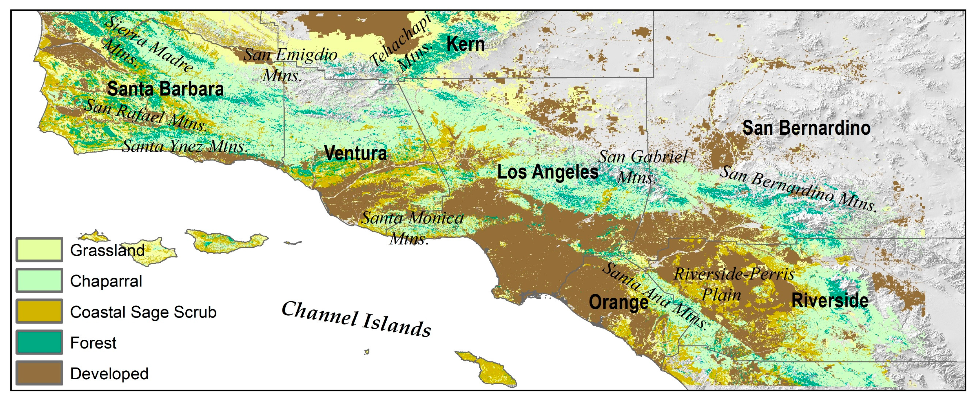
2.1. Study Area

The study area, located in the U.S. Pacific Southwest, occupies the major part of Southern California, (Figure 1, Lat. 121–116°W, Lon. 33–35°N), covering a land area of approximately 57,600 km². It is mainly comprised of four physiographic provinces: the Transverse Ranges extending from northwest to central east, the Peninsular Ranges at the southeast end, the low-lying Los Angeles Basin between the two coastal ranges, and the Mojave Desert at the northeast corner [40]. The topography of this region is rugged and complex. The lowest coastal plains (<400 m a.s.l.) and the relatively higher inland desert (600–1200 m a.s.l.) are interrupted by a stretch of mountains (>1200 m a.s.l.). The coastal and mountainous regions are predominately controlled by a Mediterranean climate with mild, wet winters and warm, dry summers. In the narrow south coast and the southeast lowland, the Mediterranean climate gives way to a semi-arid climate, which is drier and where evaporation exceeds precipitation throughout the year. Both temperature and precipitation demonstrate variation with latitude and elevations. Further north and from the coast to the mountains, precipitation increases from 300 mm/yr to more than 800 mm/yr and annual mean temperature decreases from 20 °C to less than 8 °C. The Mojave Desert, which lies in the rain shadow of the Sierra Nevada Mountains and the Transverse Ranges, has a dry desert climate, receives limited precipitation (less than 300 mm/yr). The annual temperature ranges between 16–20 °C [55].

The land cover distribution reflects the rugged topography and the diversity in climate, with the more forested area at the tops of the Transverse Ranges; principally developed, cultivated lands or oak woodlands, shrublands and grasslands over the lower plains; and vast desert scrubs over the Mojave Desert (Figure 2). The coastal mountains are dominated by CSS and chaparral communities, both of which are mainly composed of drought-tolerant species. However, CSS plants are generally shallow-rooted and drought-deciduous, compared to the mostly evergreen chaparral [39]. Due to the extremely dry summers, Southern California is a fire-prone region. Fire is a significant vegetation disturbance, which can degrade chaparral communities to grasslands abruptly. Shrub canopies recover in the following years; nevertheless, the post-fire regeneration largely depends on the fire intensity [57,58].

2.2. Data Sets

2.2.1. Vegetation Index Dataset

Satellite-derived Normalized Difference Vegetation Index (NDVI) data at a spatial resolution of 250 m and a temporal resolution of 16 days were acquired from the Moderate Resolution Imaging Spectroradiometer (MODIS) sensor, distributed by NASA’s Earth Observing System Data and Information System (https://reverb.echo.nasa.gov/). The time span of the MOD13Q1 NDVI products (Collection 6, tile h08v05) cover from 18 February 2000 to 22 April 2017 [59]. The data after spring 2017 were excluded from this study, because of the extreme fire seasons in 2017 and 2018 (e.g., the Thomas Fire [60] and the Woolsey Fire [61]). These fires abruptly decreased the NDVI of large areas and hindered the analysis of climatic and drought effects.

We conducted some preprocessing for the NDVI data to ensure the reliability of this study. The pixels with negative NDVI values, which denote little or no vegetation (e.g., completely built-up urban areas), were removed before analysis. As snow tends to lower the NDVI [62], MODSCAG snow covered-area data [63], provided by NASA Jet Propulsion Laboratory, were applied to mask the NDVI pixels that had average snow fractions of more than 1% during a 16-day period. To match the temporal resolution of the drought index, the 16-day NDVI time-series were resampled to monthly time-series, by averaging the available tiles in each calendar month at each pixel.

2.2.2. Drought Index and Climate Variables

The monthly gridded, self-calibrated Palmer Drought Severity Index (PDSI) data set with a spatial resolution of 4 km was downloaded from the WestWide Drought Tracker website ([64]; WWDT, https://wrcc.dri.edu/wwdt/). PDSI is the most prominent index of meteorological drought in the United States [65], which incorporates antecedent precipitation, moisture supply, and moisture demand into a hydrologic accounting system [66]. Negative (positive) PDSI values indicate a drought (wet) period, and PDSI <−2, <−3, and <−4 refer to moderate, severe, and extreme drought, respectively [67]. Parameter-elevation Regression on Independent Slopes Model (PRISM, http://prism.oregonstate.edu; [68]) climate data serves as the foundational data set for computing the WWDT drought index. United States Historical Climatology Network (USHCN) data and Penn State STATSGO soil water holding capacity data also contributed to the climate data adjustment and the soil water balance calculations respectively [64]. The WWDT drought data has been intensively applied to climatological and hydrological studies in recent years (see [69,70,71,72,73,74,75]), and has been proved with good reliability. To match the spatial resolution of the MODIS NDVI maps, the PDSI dataset was interpolated to a 250 m × 250 m resolution using bilinear interpolation. The uncertainties and limitations of the data rescaling are discussed in Section 4.

The 30-year monthly PRISM Normals of temperature and precipitation were used in this study to demonstrate the normal climate conditions over the space of the study area [55]. This data set covers the period of 1981–2010 and has an initial spatial resolution of 800 m, which was rescaled on 250 m grids using bilinear interpolation. In addition, the monthly Daymet climate data set (version 3) on a 1 km grid was used to elucidate the climate change background for the period 1980–2017 in Southern California ([76]; https://daymet.ornl.gov/). The long-term trends of monthly averages of maximum temperature, minimum temperature, as well as monthly total precipitation were analyzed.

2.2.3. Ancillary GIS Data

Fire perimeter data for the period January 2000–April 2017 were provided by the Department of Forestry and Fire Protection of California’s Fire and Resource Assessment Program (FRAP, http://frap.fire.ca.gov/). The FRAP compiled this statewide spatial database of fire perimeters from BLM (US Bureau of Land Management), NPS (National Park Service), and USFS (US Forest Service) fires. The FRAP fire database represents the best digital record of fire history in California, and its data quality is higher than that of MODIS fire data or other data sets [77,78]. The California State Wildlife Action Plan (SWAP; https://www.wildlife.ca.gov/SWAP) data were applied to identify the vegetation polygons of chaparral, CSS, grassland, forest, and developed land over Southern California [79]. The SWAP land cover data provides information on the distribution of vegetation types with high spatial resolution (30 m resolution) (Figure 2). We follow [80] and the SWAP data were aggregated to a 250 m × 250 m resolution using majority statistics. This means that the vegetation type for each MODIS pixel was identified as the type that had the highest frequency at 30 m resolution in each 250 m × 250 m grid. This approach better reflects the regional vegetation distribution than the nearest-neighbor interpolation, and is less affected by data noise and misclassifications [80]. Additionally, a rigorous data quality control was implemented by the California Department of Fish and Wildlife in generating the SWAP database and, thus, it is the “best available” land cover data for California at present [50]. Vegetation cover typical of chaparral is comprised of sclerophyllous, evergreen-leaved shrubs with hard stems and deep roots with a variety of species. CSS is dominated by softer-leaved, woody shrubs and sub-shrubs. The rooting zone is shallower than chaparral and the dominant shrubs may be summer deciduous or possess smaller leaves during the dry season. Grasslands are typically dominated by a variety of non-native annual grasses, which die in the summer months and the cover regenerates through seed germination in the winter. Lower-elevation stands of woodland-forests are dominated by evergreen and deciduous oak, while the higher elevations (>1300 m a.s.l.) are mainly occupied by conifer stands (e.g., pines and firs).

2.3. Methodology

The monthly time-series of NDVI anomalies at the 250 m pixel level of resolution was calculated for the period from February 2000 to April 2017. Then, Pearson’s correlations and linear regressions were performed between the NDVI anomalies and PDSI for each pixel. The NDVI–PDSI regression slopes represent the vegetation sensitivity to drought, and the NDVI–PDSI correlation coefficients indicate the strength of the relationships between the vegetation greenness and water availability. Correlation and regression analyses between NDVI and PDSI were also calculated for different seasons: winter, December–February; spring, March–May; summer, June–August; and fall, September–November. All the correlation and regression coefficients were tested at a 95% confidence level.

To detect long-term trends in the browning or greening of the vegetation over the past 17 years, a Theil–Sen estimator was utilized to measure the changing trends of the pixel-wise NDVI. The Theil–Sen algorithm is a robust trend detection approach, which gives the median changing slope of a time-series and, thus, is less affected by outliers than parametric approaches [81,82]. Though the NDVI time-series also contains some fluctuations induced by short-term disturbances (e.g., fire or diseases), the Theil–Sen method is appropriate for capturing the long-term greenness trends attributed to climate change. The Mann–Kendall test was applied to identify the significance of the NDVI trends. As a non-parametric test, the Mann–Kendall test is a reasonable method for detecting monotonic trends in series of environmental data, climate data, or hydrological data, regardless of the distribution of the data [83,84,85]. Given that autocorrelations commonly exist in environmental time-series, we used the pre-whitening algorithm proposed by [86] to remove the lag-1 serial correlations in the anomaly NDVI time-series before trend detection. Existence of a serial correlation can increase the probability that the Mann–Kendall test detects a significant trend, leading to a disproportionate rejection of the null hypothesis of no trend [87]. We also applied the same trend detection procedure to the monthly time-series of maximum temperature, minimum temperature, and precipitation, which indicated the recent climate change background in Southern California.

To compare the relative sensitivity of the five vegetation communities to drought, a dummy variable regression was performed, which uses the regression slopes between NDVI anomalies and PDSI as the dependent variable and vegetation as the unique predictor. Vegetation in developed land was selected as the reference category, as it showed the smallest seasonal variations. The dummy regression model gives the relative changes in NDVI–PDSI regression slopes for forest, chaparral, CSS, and grassland, as compared to developed land. By comparing the drought sensitivity of natural and developed-land vegetation, we may estimate how human activities mitigate the drought impact on urban vegetation and verify the assumption that natural vegetation is more vulnerable to drought than vegetation in developed lands.

Moreover, we employed multiple linear regression to further investigate the geographically different vegetation response to drought caused by climate, using the regression slopes between NDVI anomalies and PDSI as the dependent variable, while normal temperature and precipitation were the independent variables. As multiple linear regression assumes the independent variables are not highly correlated with each other, we used variance inflation factor (VIF) to detect multicollinearity [88]. A general rule is that the VIF should not exceed 10 to avoid severe multicollinearity [89]. Based on the two-fold regression, we can identify the impact of changing temperature and precipitation on the drought sensitivity of the vegetation types. To remove the influence of wildfire, we discarded all burned pixels over the study period, which were identified according to the FRAP fire perimeter data. As there are about 1 million MODIS pixels in this area, the large sample size may result in overestimation of minuscule effects in statistical analysis [90], represented by extremely small p-values. To overcome this problem, two solutions were utilized: first, a bootstrapping approach was applied to conduct the multiple linear regression, and within each of the total 1000 replicates, only 500 pixels were randomly selected to derive the regression coefficients and p-values; second, the standardized regression coefficient (slope) for each predictor in each bootstrapping replicate was also calculated as an effect size index [91]. The standardized slopes were calculated as

β^s_j = β_j × SD(X_j) / SD(Y),

(1)

where β_j are the raw regression slopes and SD(X_j) and SD(Y) are the standard deviations of the independent variables (normal temperature and precipitation) and dependent variables (regression slopes between NDVI anomalies and PDSI), respectively. Standardized slopes in multiple regression analysis are scale-free estimates of the effect of a focal predictor on a target outcome [92]. These estimates are comparable in magnitude within different models and studies, and thus have advantages over partial correlation coefficients [93]. Therefore, the standardized slopes are more appropriate for demonstrating the impacts of the climate gradient on vegetation drought-tolerance than the raw regression slopes, and facilitate the comparison between temperature and precipitation contributions.

3. Results

3.1. Vegetation Dynamics and Relationships with Drought

As indicated by the decreasing PDSI, the Californian climate has become drier over the past 30 years, where the relative drying on the south coast has been stronger than the rest of the state (Figure 3). An extreme water deficit can exert negative impacts on ecosystem health, as the observed decline in vegetation greenness. Due to the persistent drying (Figure 3) and frequent wildfires (Figure 1) in Southern California, the natural vegetation might be expected to display general browning. Pixel-wise Theil–Sen’s slopes of NDVI represent the greening or browning of the vegetation (Figure 4). The burned regions showed the most abrupt NDVI declines at the rate more than 0.009/yr (Figure 4). However, browning was not constrained to burned sites. Besides the fire disturbances, the severe browning along the Californian south coast could mainly be attributed to climate disturbances. The spring (MAM) and summer (JJA) images show the greatest NDVI declines. The most severely browned regions include west Riverside County (more than 0.009/yr in spring), southwest Kern County (more than 0.007/yr in spring), south Los Angeles County (0.003–0.005/yr in spring and summer), and the western Transverse Ranges (more than 0.005/yr in all seasons).

Though all the five major vegetation types showed stronger NDVI decline (

Table 1. Median NDVI Theil–Sen’s slopes for the major vegetation types.

Vegetation Type	Trend (Winter)	Trend (Spring)	Trend (Summer)	Trend (Fall)
Chaparral	−0.0078	−0.0082	−0.0080	−0.0078
Coastal Sage Scrub (CSS)	−0.0051	−0.0083	−0.0051	−0.0051
Annual and Perennial Grassland	−0.0040	−0.0078	−0.0030	−0.0040
Forest and Woodland	−0.0065	−0.0055	−0.0061	−0.0065
Developed Land	−0.0027	−0.0033	−0.0029	−0.0027

), there were some seasonal differences between them. CSS (−0.0083/yr) and grassland (−0.0078/yr) showed greater NDVI declines in spring than the other seasons and vegetation communities. Chaparral showed strong browning across all four seasons. The fact that chaparral and forest did not display apparent seasonal variations in the NDVI trends might be related to their deep-rooted features. CSS and grassland communities displayed less browning than chaparral and forest in summer and fall. The chaparral communities (−0.0078–−0.0082/yr) and the developed-land vegetation (−0.0033–−0.0027/yr) showed the largest and smallest NDVI declines, respectively, throughout the year (see Table 1).

The significant correlations and regressions between NDVI anomalies and PDSI for all seasons in nearly all pixels suggest that the vegetation was very sensitive to drought in this region (Figure 5 and Figure 6). The strongest correlations were found in the summer months (June–August), while the highest regression slopes were shown in winter (December–February). The Mediterranean climate can account for this seasonal pattern (i.e., most of the precipitation and vegetation growth occurs in winter, and all the natural plants must endure water scarcity in summer). In consequence, moderate magnitudes of the correlation (0.47–0.62) and regression coefficients (0.0109–0.0204) between NDVI and PDSI for the natural vegetation were observed for spring (March–May) and fall (September–November) as transitional periods (

Table 2. Median correlation coefficients (r) between NDVI anomalies and PDSI for the major vegetation types.

Vegetation Type	r (Winter)	r (Spring)	r (Summer)	r (Fall)
Chaparral	0.45	0.58	0.69	0.60
Coastal Sage Scrub (CSS)	0.52	0.62	0.74	0.61
Annual and Perennial Grassland	0.42	0.53	0.61	0.47
Forest and Woodland	0.39	0.48	0.61	0.52
Developed land	0.34	0.36	0.37	0.35

and

Table 3. Median regression slopes (β) between NDVI anomalies and PDSI for the major vegetation types.

Vegetation Type	β (Winter)	β (Spring)	β (Summer)	β (Fall)
Chaparral	0.0143	0.0146	0.0148	0.0169
Coastal Sage Scrub (CSS)	0.0212	0.0204	0.0116	0.0149
Annual and Perennial Grassland	0.0215	0.0192	0.0070	0.0118
Forest and Woodland	0.0125	0.0109	0.0104	0.0128
Developed land	0.0069	0.0057	0.0044	0.0062

).

Although desert vegetation is adapted to low moisture availability, the vegetation greenness in the Mojave Desert (northeast study area) showed surprisingly strong positive correlations with PDSI, indicating vegetation sensitivity to moisture stress there (Figure 5). However, the regression slopes were smaller compared to the coast, perhaps due to lower relative sensitivity and the already scarce vegetation and lower NDVI value in the desert (Figure 6). Weak correlations and high regression coefficients were found in the burned regions, which can be attributed to abrupt fire disturbances (Figure 5 and Figure 6). For example, wildfires in drought years may largely reduce the NDVI of the burned areas, and when precipitation rebounds after drought, post-fire regeneration can bring a rapid increase in NDVI. Besides the desert and burned areas, the vegetation in the coastal mountain ranges demonstrated striking relations with the PDSI (e.g., in the San Rafael Mountains, Santa Ynez Mountains, Santa Monica Mountains, Santa Ana Mountains, and Riverside-Perris Plain).

We found that most of the browning regions showed close relationships between NDVI anomalies and PDSI (Figure 4 and Figure 5). This is consistent with the general browning in Southern California due to decreasing PDSI during recent years (Figure 3). As a measurement of dryness based on precipitation and temperature, reduction of precipitation and elevated temperature can both decrease PDSI. A large portion of Southern California has shown an appreciable warming trend in all seasons over the past 37 years (Figure 7 and Figure 8). A few regions near the San Emigdio Mountains displayed cooling in the night (decreased minimum temperature), which was offset by stronger daytime warming. At the same time, precipitation did not generally demonstrate significant changes, with only the southwest Mojave Desert showing decreased precipitation in spring (Figure 9).

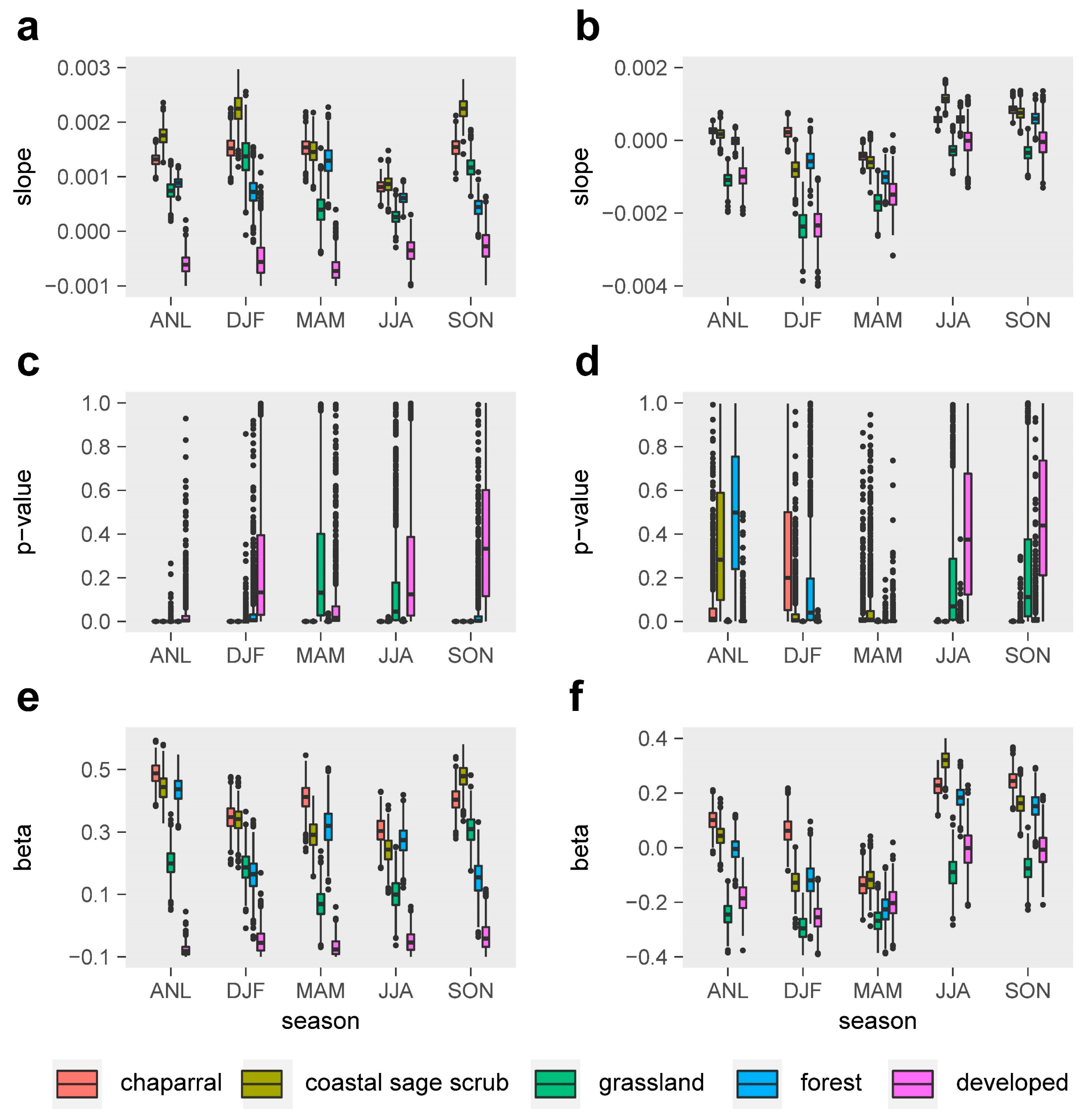
3.2. Relative Sensitivity of the Major Vegetation Types

Due to varied responses of the five vegetation communities to drought and increasing temperatures/aridity, the regression slopes between NDVI anomalies and PDSI varied among vegetation types. The relative sensitivity of the vegetation also displayed seasonal differences (Figure 10). Compared to developed land, grassland and CSS showed significantly increased drought sensitivity in winter and spring, and a mild increase of drought sensitivity in summer and fall (Figure 10 and Table 3). Grassland had the largest seasonal fluctuations in response to drought stress (Table 3). Chaparral showed the highest drought sensitivity in the warm seasons (median p < 0.05, Figure 10 and Table 3). Forest displayed an insignificant increase in drought sensitivity, compared to developed land, in the cold seasons, but a significantly increased sensitivity from summer to fall (Figure 10).

The seasonal correlation coefficients between NDVI anomalies and PDSI reflected the general water stress variations of the five vegetation types throughout the year (Table 2). Winter (summer) showed the lowest (highest) median correlation coefficients, indicating less severe (extreme) drought stress due to favorable (limited) water conditions. Spring and fall displayed intermediate correlation coefficients, suggesting moderate drought stress. Moreover, the NDVI–PDSI correlations also displayed slight differences among the five ecosystems (Table 2). Chaparral and CSS showed relatively higher correlation coefficients in all seasons, indicating that the two communities had a more consistent response to drought in time, as compared to forest, grass, and developed land.

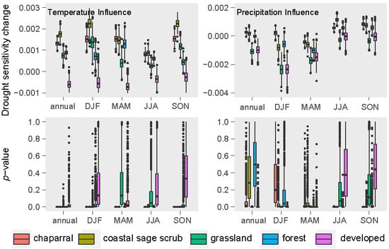
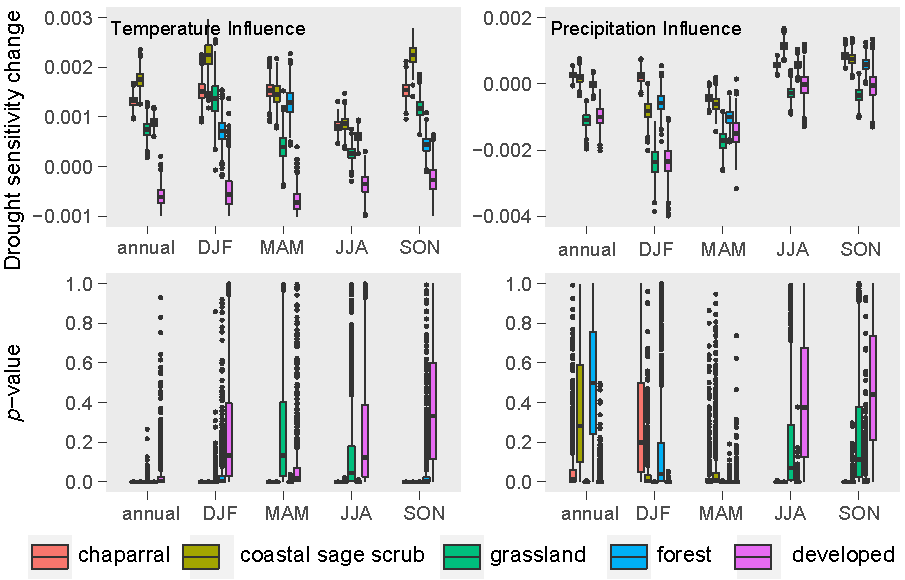
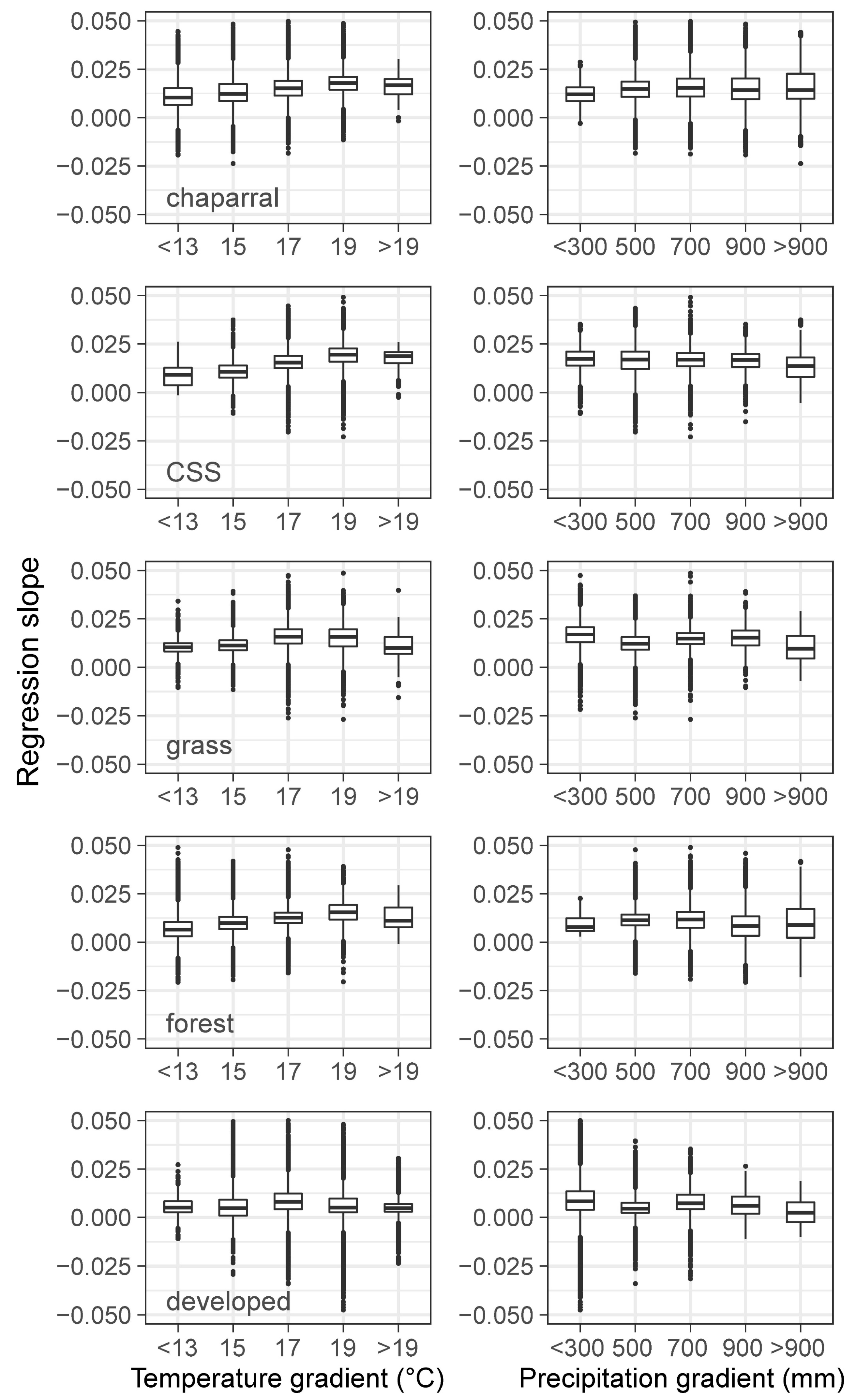
3.3. Climatic Effects on Shifting the Drought Impacts

The spatial variations of the NDVI–PDSI regression slopes of the four natural vegetation types against the normal temperature and precipitation gradients suggest that all the regression slopes increased in geographic regions with higher temperatures but remained stable across geographic precipitation gradients (Figure 11). In other words, natural vegetation in the warmer regions of the study area were more sensitive to drought, as indicated by their larger NDVI–PDSI regression slopes. However, the spatial precipitation patterns did not demonstrate a similar geographic influence. Additionally, the vegetation in developed lands seems to be less affected by temperature or precipitation changes (Figure 11).

The bootstrapped regressions indicate that the standardized slopes (beta) against precipitation were smaller than those of temperature for all the major vegetation types (Figure 12). We calculated the variance inflation factor (VIF) for all the multiple linear regressions (Figure S1). All the VIFs were <1.5, and thus these regressions did not violate the assumption of no multicollinearity [89]. The beta values of precipitation mainly ranged between −0.3 and 0.3, which denotes that one SD (standard deviation) precipitation change would only induce <0.3 SD change of the regression slopes between NDVI anomalies and PDSI. In contrast, a 1 SD temperature increase would raise the NDVI–PDSI regression slopes by up to 0.5 SD. Additionally, precipitation showed opposite effects in changing the vegetation sensitivity between the wet and dry seasons. In other words, more precipitation could decrease the NDVI–PDSI slopes in winter and spring, and increase them in summer and fall, resulting in insignificant annual effects (p > 0.05) for most vegetation communities, except for grassland (Figure 12). Temperature demonstrated significant (p < 0.05) and positive beta values in nearly all bootstrapped regressions (seasonal and annual), except for grassland in spring and summer, as well as developed land in all seasons. Thus, warmer temperatures consistently increased the natural vegetation sensitivity to drought, and the effects were prone to be greater in the dry season. Strikingly, the chaparral communities displayed very high median standardized slopes of temperature (>0.3 SD, p < 0.05) in all seasons (Figure 12e).

4. Discussion

Our analysis reveals the relative sensitivity of five major wildland vegetation types and developed areas to increased warming and aridity in Southern California, a Mediterranean climate region. Climatic water deficit (CWD), which combines the influences of temperature and precipitation, has been shown to be an important driver of woody plant decline and mortality in drought [94], which is consistent with the results presented here. Quetin and Swann [95] recently investigated the impacts of changing temperature and precipitation on global NDVI. Here, we further focus on how a changing climate will affect vegetation drought sensitivity. The bootstrapped multiple regression model utilized in our study dissociated the effects of temperature and precipitation on drought stress, and allowed for examination of the seasonal variations of these effects. The bootstrapping approach successfully reduced the overestimation of minuscule effects, which generally occurs in big data (e.g., remotely sensed data) analytics [90]. Precipitation consistently showed more insignificant results in predicting vegetation sensitivity to drought, while temperature displayed significant effects in nearly all bootstrapped regressions.

Previously, [23] has found that the forests in southwest U.S. are particularly sensitive to the increasing aridity and warmth. We further compared the differential responses of drought sensitivity (NDVI–PDSI regression slopes) to temperature and precipitation changes in forest, shrubs, grass, and developed land. All the natural vegetation types showed greater sensitivity in the warmer areas of the region, implying that temperature increases alone will be an important determinant of vegetation vulnerability to global warming in the 21st century. Vegetation in developed lands were consistently less responsive to warming, indicating the effects of irrigation in droughts, although winter precipitation increases seem to be able to reduce drought sensitivity in urban vegetation (Figure 12f). Grasslands showed less sensitivity in response to the combined effects of high temperatures and drought stress; while chaparral displayed very high sensitivity in all seasons. Thus, grassland and chaparral seem to be the most resistant and vulnerable communities, respectively, to drought under the effects of a warmer climate (Figure 12e). This is consistent with a recent study by [96], who concluded that forest and grass displayed longer and shorter drought legacy effects, respectively, but both showed greater drought resilience than shrubs. These differences arise from different eco-hydrological and physiological responses of these plant’s functional groups (e.g., rooting systems, water-use patterns, and differential hydraulic responses).

It should be mentioned that uncertainties exist in the relationship between extreme events in climate and vegetation (e.g., non-linearities and time lags), but pixels having more drought stress should have experienced more vegetation extremes and, therefore, the slopes of the NDVI–PDSI linear regressions could be used as an indicator of apparent sensitivity [51]. Another limitation of this study is related to the inconsistency of the databases used, in terms of spatial resolution. Bilinear interpolation was used in rescaling the PDSI and PRISM climate normals to MODIS resolution. For these continuous variables, bilinear interpolation can provide more accurate predictions than the other simple resampling approaches, such as nearest neighbor interpolation, and it has been widely used to rescale climate variables in similar studies, e.g., [97,98,99,100]. Some researchers have developed statistical or dynamical downscaling techniques for climate variables, e.g., [101,102]. However, as the space-time variability and patterns of a climate variable are highly dependent on the location of this variable, it is not practical to directly apply a downscaling approach developed for another region to our study region, or to use a downscaling approach for all climate variables. In addition, as PDSI reflects the variations of many climate variables (e.g., temperature, precipitation, evaporation, soil moisture, and wind speed), there is still no ready-to-use downscaling method for PDSI. Moreover, [17] analyzed how spatial resolution changes affect the relationship between PDSI and NDVI, and they found that the NDVI–PDSI correlations and regression coefficients did not change much when the data resolution was adjusted from 4 km to 500 m. Besides the spatial resolution issue, uncertainties may arise from the differential temporal resolution of PDSI and NDVI data. To match the PDSI time step, we adjusted the MODIS NDVI data set from 16-day to monthly. The higher frequency of the NDVI observations can capture more vegetation dynamics. However, as this study was focused on climatological analysis, and as the three droughts in Southern California during 2000–2017 were all prolonged droughts (2–4 years), the degraded temporal resolution of MODIS NDVI should only have little influence on the results included in this paper. Thus, we assume the uncertainties and biases induced by the different data resolutions cannot largely change the conclusions presented here. In addition, the lagged relationship between hydrological variables (precipitation, soil moisture, and drought) and vegetation growth also brings uncertainties to this study. Compared to the newly developed drought indices, such as the standardized precipitation index (SPI) and the standardized precipitation evapotranspiration index (SPEI), PDSI is limited by its fixed time scale of one month. However, the PDSI of a given month can represent an accumulation of drought over the previous few months and is highly correlated with the top 1 m soil moisture [103,104]. SPI is calculated solely based on precipitation and does not take temperature influence into account. SPEI is better than PDSI in reflecting the variations of soil moisture and evapotranspiration in drought and is superior for its varying time scales [103]. As a traditional drought index, PDSI has long been used for drought measurement and has advantages in providing comparable results with other related studies, e.g., [15,16,105,106]. As [107] suggested, no single drought index can capture all aspects of soil moisture drought. An interesting work in the future would be investigating the vegetation responses to drought and climate change using other drought indices and varying time scales.

Previous studies (e.g., [108,109,110,111]) have suggested that the sprawling development pattern in Southern California has been an important driver of contemporary chaparral conversion to herbaceous cover, both through the direct removal and fragmentation of habitat, but also through its indirect role in driving annual grass expansion associated with shortened fire intervals. As we have excluded the burned areas in this study, the NDVI change analyses should not be affected by the wildfires. As the SWAP land cover map is a recently updated (in 2015) database, the areas newly occupied by residents were identified as developed lands, instead of as natural vegetation. Thus, the NDVI trends and vegetation sensitivity for the developed lands in this study may include some signals of type conversion from natural vegetation communities to urban vegetation. However, as our study is limited to the MODIS era (after 2000), the uncertainties due to vegetation type conversions are restrained and should not alter the main conclusions.

Relative differences in the drought and temperature sensitivities of the five wildland vegetation types and their related seasonal changes in NDVI also reflect their different phenological characteristics. For example, the annual Californian grassland and summer deciduous or dimorphic CSS are well-adapted to the summer drought of the Mediterranean climate; as they die back, they become dormant or reduce photosynthesis when the soil moisture significantly decreases in summer [40]. In the cool and humid winter, the two communities reach maximum biomass quickly. By contrast, chaparral and forest trees consist of many evergreen species, which carry on photosynthesizing over the summer months and show less seasonality [40]. As a result, the CSS and grassland flora displayed higher NDVI–PDSI regression slopes than the chaparral and forest communities in winter and spring and lower slopes from summer through fall, partly because of the seasonally low NDVI of the two former communities in the warm season (Figure 10).

Climate trend detection suggests an intense warming in the region since 1980s, especially in summer and fall, when the most extreme seasonal water shortage occurs (Figure 7 and Figure 8). At the same time, precipitation did not display any meaningful trends, except for a slight decrease over the Southern Mojave Desert in spring. Previous studies suggest that the differing drought intensities and inter-annual variations of precipitation in Northern and Southern California are related to a hydroclimatic dipole [17,112]. Both the historical observations and the future projections support a more severe drying in Southern California than the north [17,113]. Within Southern California, it is still not clear what factors are controlling the spatial patterns of the drying and warming trends. Both the large-scale atmospheric circulation and the regional-scale land surface conditions (e.g., topography, albedo, soil moisture, and land covers) are potential influences.

The recent warming seems to be an important component in any long-term trends in browning over Southern California (Figure 4). There were also a few regions at higher elevations (>1500 m a.s.l.) that demonstrated greening trends over the past 17 years (Figure 4). The greening of the cold-limited montane vegetation (mainly in winter) might be caused by climate warming (i.e., due to the favorable temperature and earlier snowmelt) [114]. In addition, it is still not clear why some highly elevated areas over the San Emigdio Mountains showed significant night cooling and daytime warming (Figure 8). As a fire-prone region (Figure 1), it should be mentioned that an abrupt vegetation removal by wildfires may create a more arid environment with enhanced diurnal temperature fluctuations, i.e., increasing the temperature in daytime but decreasing it at night [54]. Moreover, since chaparral shrubs are susceptible to freezing injury [115], persistent night cooling of the San Emigdio Mountains may be as harmful as high temperatures and drought to the wildely distributed chaparral plants in this region.

Jacobsen and Pratt [116] found that the Southern California shrublands are relatively resilient to short-term high-intensity droughts, but displayed significant dieback and mortality during the recent prolonged drought (2012–2016); they concluded that the highly cavitation-resistant shrubs are the ones most affected by long-term high-intensity drought. This is supported by [50], who argued that the deep-rooting system of chaparrals buffers them from summer drought but makes them particularly vulnerable to multi-year drought, where the soil water stored in the deep layers is reduced by persistent evaporation. Our results further reveal that the chaparral communities seem to be less resilient to climate disturbance than the other vegetation types. They will likely be impacted more severely by future climatic warming and drying, due to their highest overall sensitivity to drought stress exacerbated by annual temperature increases (Figure 12e). Previously, [50] found that the cooler and moister climate at high elevations of the Californian south coast could produce decreased sensitivity of chaparral to drought but did not change the sensitivity of CSS. However, coastal fog might weaken the temperature effects on drought stress in CSS [50]. In this paper, we extended the study area to the inland Southern California mountains, and high temperatures, indeed, displayed a significant effect of increasing drought impacts on CSS in all seasons (Figure 12). Thus, the drought stress of the CSS plants, particularly where fog is limited, will probably also increase under a warmer future climate. In the following work, we are going to apply this analysis to other Mediterranean-climate regions exposed to drought, and disentangle the effects of snow, fire, groundwater level changes, and low temperature extremes for the mountainous areas. Moreover, it is important to further reveal the role of root depth in modulating the drought sensitivity of the Mediterranean-climate ecosystems.

In response to the increasing aridity and frequent fires, the Southern Californian ecosystems may shift over time, perhaps favoring grasslands and generally lower biomass covers [14,117]. As previously noted, any replacement of woody vegetation by grasslands or developed lands will alter ecosystem services, through loss of certain habitat types in affected locales and increased vulnerability of slopes to erosions and landslides. Additionally, since chaparral shrubs may have an important role in holding soil water and increasing groundwater recharge (provisioning) through channel infiltration, a degradation of the chaparral community may affect the local groundwater level [118,119]. In addition to these regional impacts, vegetation transitions could impact the carbon balance. Mediterranean climate vegetation communities have been shown to be among those displaying the highest net primary productivities (NPP) amongst the world biomes [120,121], but the net ecosystem carbon exchange of Mediterranean climate vegetation is highly sensitive to drought [122,123]. Consequently, a warmer and drier climate could significantly deteriorate the carbon budget over Mediterranean climate regions, such as Southern California. Decreased vegetation productivity coupled with the loss of woody vegetation would favor the conversion to grasslands and developed lands.

5. Conclusions

In this study, we utilized a bootstrapping regression to investigate the effects of changing temperature and precipitation in modulating the drought sensitivity of Mediterranean ecosystems in Southern California. The main conclusions are summarized as follows:

(1)

Temperature increase can significantly aggravate the susceptibility of the major Mediterranean-climate vegetation types to drought. The recent greenness declines may be related to the synchronous compound influence of high temperatures and drought.

(2)

Precipitation changes display insignificant or less effects in adjusting the vegetation sensitivity to drought.

(3)

Chaparral seems to be the most vulnerable community to the future hot droughts in all seasons, and CSS will likely be more sensitive to drought from fall to winter under a warmer climate. Climate warming may only exert small effects in grassland and developed-land vegetation.

References

1. Lau, W.K.M.; Wu, H.-T.; Kim, K.-M. A canonical response of precipitation characteristics to global warming from CMIP5 models. Geophys. Res. Lett. 2013, 40, 3163–3169. [Google Scholar] [CrossRef]
2. Mariotti, A.; Pan, Y.; Zeng, N.; Alessandri, A. Long-term climate change in the Mediterranean region in the midst of decadal variability. Clim. Dyn. 2015, 44, 1437–1456. [Google Scholar] [CrossRef]
3. IPCC (Intergovernmental Panel on Climate Change). Climate Change 2007—The Physical Science Basis: Working Group I Contribution to the Fourth Assessment Report of the IPCC; Cambridge University Press: Cambridge, UK, 2007. [Google Scholar]
4. Cook, B.I.; Smerdon, J.E.; Seager, R.; Coats, S. Global warming and 21st century drying. Clim. Dyn. 2014, 43, 2607–2627. [Google Scholar] [CrossRef] [Green Version]
5. Frank, A.B.; Karn, J.F. Vegetation Indices, CO2 Flux, and Biomass for Northern Plains Grasslands. J. Range Manag. 2003, 56, 382. [Google Scholar] [CrossRef]
6. Klausmeyer, K.R.; Shaw, M.R. Climate Change, Habitat Loss, Protected Areas and the Climate Adaptation Potential of Species in Mediterranean Ecosystems Worldwide. PLoS ONE 2009, 4, e6392. [Google Scholar] [CrossRef] [PubMed] [Green Version]
7. Gabet, E.J.; Dunne, T. Landslides on coastal sage-scrub and grassland hillslopes in a severe El Niño winter: The effects of vegetation conversion on sediment delivery. Geol. Soc. Am. Bull. 2002, 114, 983–990. [Google Scholar] [CrossRef]
8. Costa-e-Silva, F.; Correia, A.C.; Piayda, A.; Dubbert, M.; Rebmann, C.; Cuntz, M.; Werner, C.; David, J.S.; Pereira, J.S. Effects of an extremely dry winter on net ecosystem carbon exchange and tree phenology at a cork oak woodland. Agric. For. Meteorol. 2015, 204, 48–57. [Google Scholar] [CrossRef] [Green Version]
9. Ma, S.; Baldocchi, D.D.; Xu, L.; Hehn, T. Inter-annual variability in carbon dioxide exchange of an oak/grass savanna and open grassland in California. Agric. For. Meteorol. 2007, 147, 157–171. [Google Scholar] [CrossRef]
10. Frank, D.; Reichstein, M.; Bahn, M.; Thonicke, K.; Frank, D.; Mahecha, M.D.; Smith, P.; van der Velde, M.; Vicca, S.; Babst, F.; et al. Effects of climate extremes on the terrestrial carbon cycle: concepts, processes and potential future impacts. Glob. Chang. Biol. 2015, 21, 2861–2880. [Google Scholar] [CrossRef] [Green Version]
11. Grant, R.F.; Baldocchi, D.D.; Ma, S. Ecological controls on net ecosystem productivity of a seasonally dry annual grassland under current and future climates: Modelling with ecosys. Agric. For. Meteorol. 2012, 152, 189–200. [Google Scholar] [CrossRef]
12. Baldwin, B.G. Origins of Plant Diversity in the California Floristic Province. Annu. Rev. Ecol. Evol. Syst. 2014, 45, 347–369. [Google Scholar] [CrossRef] [Green Version]
13. Kauffman, E. Climate and topography. In Atlas of the Biodiversity of California; California Department of Fish and Game: Sacramento, CA, USA, 2003. [Google Scholar]
14. Lenihan, J.M.; Bachelet, D.; Neilson, R.P.; Drapek, R. Response of vegetation distribution, ecosystem productivity, and fire to climate change scenarios for California. Clim. Change 2008, 87, 215–230. [Google Scholar] [CrossRef]
15. Griffin, D.; Anchukaitis, K.J. How unusual is the 2012-2014 California drought? Geophys. Res. Lett. 2014, 41, 9017–9023. [Google Scholar] [CrossRef] [Green Version]
16. Williams, A.P.; Seager, R.; Abatzoglou, J.T.; Cook, B.I.; Smerdon, J.E.; Cook, E.R. Contribution of anthropogenic warming to California drought during 2012–2014. Geophys. Res. Lett. 2015, 42, 6819–6828. [Google Scholar] [CrossRef] [Green Version]
17. Dong, C.; MacDonald, G.M.; Willis, K.; Gillespie, T.W.; Okin, G.S.; Williams, A.P. Vegetation Responses to 2012–2016 Drought in Northern and Southern California. Geophys. Res. Lett. 2019, 46, 3810–3821. [Google Scholar] [CrossRef]
18. Garfin, G.; Jardine, A.; Merideth, R.; Black, M.; LeRoy, S. Assessment of Climate Change in the Southwest United States; Garfin, G., Jardine, A., Merideth, R., Black, M., LeRoy, S., Eds.; Island Press/Center for Resource Economics: Washington, DC, USA, 2013; ISBN 978-1-59726-420-4. [Google Scholar]
19. MacDonald, G.M. Water, climate change, and sustainability in the southwest. Proc. Natl. Acad. Sci. USA 2010, 107, 21256–21262. [Google Scholar] [CrossRef] [Green Version]
20. Woodhouse, C.A.; Meko, D.M.; MacDonald, G.M.; Stahle, D.W.; Cook, E.R. A 1,200-year perspective of 21st century drought in southwestern North America. Proc. Natl. Acad. Sci. USA 2010, 107, 21283–21288. [Google Scholar] [CrossRef] [Green Version]
21. Diaz, H.F. Drought in the United States: Some Aspects of Major Dry and Wet Periods in the Contiguous United States, 1895–1981. J. Clim. Appl. Meteorol. 1983, 22, 3–16. [Google Scholar] [CrossRef] [Green Version]
22. Rosenzweig, C.; Iglesias, A.; Yang, X.B.; Epstein, P.; Chivian, E. Climate Change and Extreme Weather Events; Implications for Food Production, Plant Diseases, and Pests. Glob. Chang. Hum. Heal. 2001, 2, 90–104. [Google Scholar] [CrossRef]
23. Williams, A.P.; Allen, C.D.; Millar, C.I.; Swetnam, T.W.; Michaelsen, J.; Still, C.J.; Leavitt, S.W. Forest responses to increasing aridity and warmth in the southwestern United States. Proc. Natl. Acad. Sci. USA 2010, 107, 21289–21294. [Google Scholar] [CrossRef] [Green Version]
24. Sun, L.; Kunkel, K.; Stevens, L.; Buddenberg, A.; Dobson, J.; Easterling, D. Regional surface climate conditions in CMIP3 and CMIP5 for the United States: Differences, similarities, and implications for the U.S. National Climate Assessment; U.S. National Oceanic and Atmospheric Administration: Washington, DC, USA, 2015.
25. Polade, S.D.; Pierce, D.W.; Cayan, D.R.; Gershunov, A.; Dettinger, M.D. The key role of dry days in changing regional climate and precipitation regimes. Sci. Rep. 2015, 4, 4364. [Google Scholar] [CrossRef] [PubMed] [Green Version]
26. Breshears, D.D.; Cobb, N.S.; Rich, P.M.; Price, K.P.; Allen, C.D.; Balice, R.G.; Romme, W.H.; Kastens, J.H.; Floyd, M.L.; Belnap, J.; et al. Regional vegetation die-off in response to global-change-type drought. Proc. Natl. Acad. Sci. USA 2005, 102, 15144–15148. [Google Scholar] [CrossRef] [PubMed] [Green Version]
27. Adams, H.D.; Collins, A.D.; Briggs, S.P.; Vennetier, M.; Dickman, L.T.; Sevanto, S.A.; Garcia-Forner, N.; Powers, H.H.; McDowell, N.G. Experimental drought and heat can delay phenological development and reduce foliar and shoot growth in semiarid trees. Glob. Chang. Biol. 2015, 21, 4210–4220. [Google Scholar] [CrossRef] [PubMed]
28. AghaKouchak, A.; Cheng, L.; Mazdiyasni, O.; Farahmand, A. Global warming and changes in risk of concurrent climate extremes: Insights from the 2014 California drought. Geophys. Res. Lett. 2014, 41, 8847–8852. [Google Scholar] [CrossRef] [Green Version]
29. Allen, C.D.; Macalady, A.K.; Chenchouni, H.; Bachelet, D.; McDowell, N.; Vennetier, M.; Kitzberger, T.; Rigling, A.; Breshears, D.D.; Hogg, E.H. (Ted); et al. A global overview of drought and heat-induced tree mortality reveals emerging climate change risks for forests. For. Ecol. Manage. 2010, 259, 660–684. [Google Scholar] [CrossRef] [Green Version]
30. Allen, C.D.; Breshears, D.D.; McDowell, N.G. On underestimation of global vulnerability to tree mortality and forest die-off from hotter drought in the Anthropocene. Ecosphere 2015, 6, art129. [Google Scholar] [CrossRef]
31. Breshears, D.D.; Myers, O.B.; Meyer, C.W.; Barnes, F.J.; Zou, C.B.; Allen, C.D.; McDowell, N.G.; Pockman, W.T. Tree die-off in response to global change-type drought: mortality insights from a decade of plant water potential measurements. Front. Ecol. Environ. 2009, 7, 185–189. [Google Scholar] [CrossRef] [Green Version]
32. Chen, H.; Sun, J. Anthropogenic warming has caused hot droughts more frequently in China. J. Hydrol. 2017, 544, 306–318. [Google Scholar] [CrossRef]
33. Diffenbaugh, N.S.; Swain, D.L.; Touma, D. Anthropogenic warming has increased drought risk in California. Proc. Natl. Acad. Sci. USA 2015, 112, 3931–3936. [Google Scholar] [CrossRef] [Green Version]
34. Naumann, G.; Alfieri, L.; Wyser, K.; Mentaschi, L.; Betts, R.A.; Carrao, H.; Spinoni, J.; Vogt, J.; Feyen, L. Global Changes in Drought Conditions Under Different Levels of Warming. Geophys. Res. Lett. 2018, 45, 3285–3296. [Google Scholar] [CrossRef]
35. Overpeck, J.T. The challenge of hot drought. Nature 2013, 503, 350–351. [Google Scholar] [CrossRef] [PubMed]
36. Udall, B.; Overpeck, J. The twenty-first century Colorado River hot drought and implications for the future. Water Resour. Res. 2017, 53, 2404–2418. [Google Scholar] [CrossRef] [Green Version]
37. Teskey, R.; Wertin, T.; Bauweraerts, I.; Ameye, M.; Mcguire, M.A.; Steppe, K. Responses of tree species to heat waves and extreme heat events. Plant. Cell Environ. 2015, 38, 1699–1712. [Google Scholar] [CrossRef] [PubMed]
38. McDowell, N.G.; Beerling, D.J.; Breshears, D.D.; Fisher, R.A.; Raffa, K.F.; Stitt, M. The interdependence of mechanisms underlying climate-driven vegetation mortality. Trends Ecol. Evol. 2011, 26, 523–532. [Google Scholar] [CrossRef] [PubMed]
39. Barbour, M.G.; Keeler-Wolf, T.; Schoenherr, A.A. Terrestrial Vegetation of California; University of California Press: Berkeley, CA, USA, 2007; ISBN 9780520249554. [Google Scholar]
40. Holland, V.L.; Keil, D.G. California Vegetation; Kendall/Hunt Pub. Co.: Dubuque, IA, USA, 1995. [Google Scholar]
41. Barbour, M.; Pavlik, B.; Drysdale, F.; Lindstrom, S. California’s Changing Landscapes: Diversity and Conservation of California Vegetation; California Native Plant Society: Sacramento, CA, USA, 1993. [Google Scholar]
42. California Population World Population Review. Available online: http://worldpopulationreview.com/states/california/ (accessed on 4 December 2019).
43. Sleeter, B.M.; Wilson, T.S.; Soulard, C.E.; Liu, J. Estimation of late twentieth century land-cover change in California. Environ. Monit. Assess. 2011, 173, 251–266. [Google Scholar] [CrossRef] [PubMed]
44. Wilson, T.S.; Sleeter, B.M.; Davis, A.W. Potential future land use threats to California’s protected areas. Reg. Environ. Chang. 2015, 15, 1051–1064. [Google Scholar] [CrossRef] [Green Version]
45. Jamieson, M.A.; Trowbridge, A.M.; Raffa, K.F.; Lindroth, R.L. Consequences of Climate Warming and Altered Precipitation Patterns for Plant-Insect and Multitrophic Interactions. Plant Physiol. 2012, 160, 1719–1727. [Google Scholar] [CrossRef] [Green Version]
46. Richardson, A.D.; Keenan, T.F.; Migliavacca, M.; Ryu, Y.; Sonnentag, O.; Toomey, M. Climate change, phenology, and phenological control of vegetation feedbacks to the climate system. Agric. For. Meteorol. 2013, 169, 156–173. [Google Scholar] [CrossRef]
47. Klein, T.; Yakir, D.; Buchmann, N.; Grünzweig, J.M. Towards an advanced assessment of the hydrological vulnerability of forests to climate change-induced drought. New Phytol. 2014, 201, 712–716. [Google Scholar] [CrossRef]
48. Atkin, O. Thermal acclimation and the dynamic response of plant respiration to temperature. Trends Plant Sci. 2003, 8, 343–351. [Google Scholar] [CrossRef]
49. Backhaus, S.; Kreyling, J.; Grant, K.; Beierkuhnlein, C.; Walter, J.; Jentsch, A. Recurrent Mild Drought Events Increase Resistance Toward Extreme Drought Stress. Ecosystems 2014, 17, 1068–1081. [Google Scholar] [CrossRef]
50. Okin, G.S.; Dong, C.; Willis, K.S.; Gillespie, T.W.; MacDonald, G.M. The Impact of Drought on Native Southern California Vegetation: Remote Sensing Analysis Using MODIS-Derived Time Series. J. Geophys. Res. Biogeosciences 2018, 123, 1927–1939. [Google Scholar] [CrossRef]
51. Liu, G.; Liu, H.; Yin, Y. Global patterns of NDVI-indicated vegetation extremes and their sensitivity to climate extremes. Environ. Res. Lett. 2013, 8, 025009. [Google Scholar] [CrossRef] [Green Version]
52. Glenn, E.; Huete, A.; Nagler, P.; Nelson, S. Relationship Between Remotely-sensed Vegetation Indices, Canopy Attributes and Plant Physiological Processes: What Vegetation Indices Can and Cannot Tell Us About the Landscape. Sensors 2008, 8, 2136–2160. [Google Scholar] [CrossRef] [Green Version]
53. Wylie, B. Calibration of remotely sensed, coarse resolution NDVI to CO2 fluxes in a sagebrush–steppe ecosystem. Remote Sens. Environ. 2003, 85, 243–255. [Google Scholar] [CrossRef]
54. Veraverbeke, S.; Verstraeten, W.W.; Lhermitte, S.; Van De Kerchove, R.; Goossens, R. Assessment of post-fire changes in land surface temperature and surface albedo, and their relation with fire - burn severity using multitemporal MODIS imagery. Int. J. Wildl. Fire 2012, 21, 243. [Google Scholar] [CrossRef] [Green Version]
55. Daly, C.; Halbleib, M.; Smith, J.I.; Gibson, W.P.; Doggett, M.K.; Taylor, G.H.; Curtis, J.; Pasteris, P.P. Physiographically sensitive mapping of climatological temperature and precipitation across the conterminous United States. Int. J. Climatol. 2008, 28, 2031–2064. [Google Scholar] [CrossRef]
56. Rubel, F.; Kottek, M. Observed and projected climate shifts 1901-2100 depicted by world maps of the Köppen-Geiger climate classification. Meteorol. Zeitschrift 2010, 19, 135–141. [Google Scholar] [CrossRef] [Green Version]
57. Keeley, J.E.; Fotheringham, C.J.; Baer-Keeley, M. Determinants of postfire recovery and succession in Mediterranean-climate shrublands of California. Ecol. Appl. 2005, 15, 1515–1534. [Google Scholar] [CrossRef] [Green Version]
58. Keeley, J.; Davis, F. Terrestrial Vegetation of California, 3rd ed.; Barbour, M., Ed.; University of California Press: Los Angeles, CA, USA, 2007; ISBN 9780520249554. [Google Scholar]
59. Didan, K. MOD13Q1—MODIS/Terra Vegetation Indices 16-Day L3 Global 250m SIN Grid. Available online: https://ladsweb.modaps.eosdis.nasa.gov/missions-and-measurements/products/MOD13Q1/ (accessed on 4 December 2019).
60. Nauslar, N.; Abatzoglou, J.; Marsh, P. The 2017 North Bay and Southern California Fires: A Case Study. Fire 2018, 1, 18. [Google Scholar] [CrossRef] [Green Version]
61. LeComte, D. U.S. Weather Highlights 2018: Another Historic Hurricane and Wildfire Season. Weatherwise 2019, 72, 12–23. [Google Scholar] [CrossRef]
62. Hall, D.K.; Riggs, G.A.; Salomonson, V.V.; DiGirolamo, N.E.; Bayr, K.J. MODIS snow-cover products. Remote Sens. Environ. 2002, 83, 181–194. [Google Scholar] [CrossRef] [Green Version]
63. Painter, T.H.; Rittger, K.; McKenzie, C.; Slaughter, P.; Davis, R.E.; Dozier, J. Retrieval of subpixel snow covered area, grain size, and albedo from MODIS. Remote Sens. Environ. 2009, 113, 868–879. [Google Scholar] [CrossRef] [Green Version]
64. Abatzoglou, J.T.; McEvoy, D.J.; Redmond, K.T. The West Wide Drought Tracker: Drought Monitoring at Fine Spatial Scales. Bull. Am. Meteorol. Soc. 2017, 98, 1815–1820. [Google Scholar] [CrossRef]
65. Keyantash, J.; Dracup, J.A. The Quantification of Drought: An Evaluation of Drought Indices. Bull. Am. Meteorol. Soc. 2002, 83, 1167–1180. [Google Scholar] [CrossRef]
66. Heim, R.R. A Review of Twentieth-Century Drought Indices Used in the United States. Bull. Am. Meteorol. Soc. 2002, 83, 1149–1165. [Google Scholar] [CrossRef] [Green Version]
67. Palmer, W.C. Meteorological Drought; US Department of Agriculture: Washington, DC, USA, 1965.
68. Daly, C.; Gibson, W.; Taylor, G.; Johnson, G.; Pasteris, P. A knowledge-based approach to the statistical mapping of climate. Clim. Res. 2002, 22, 99–113. [Google Scholar] [CrossRef] [Green Version]
69. Balzotti, C.S.; Kitchen, S.G.; McCarthy, C. Beyond the single species climate envelope: a multifaceted approach to mapping climate change vulnerability. Ecosphere 2016, 7, e01444. [Google Scholar] [CrossRef]
70. Fei, S.; Desprez, J.M.; Potter, K.M.; Jo, I.; Knott, J.A.; Oswalt, C.M. Divergence of species responses to climate change. Sci. Adv. 2017, 3, e1603055. [Google Scholar] [CrossRef] [Green Version]
71. Kitchen, S.G.; Meyer, S.E.; Carlson, S.L. Mechanisms for maintenance of dominance in a nonclonal desert shrub. Ecosphere 2015, 6, art252. [Google Scholar] [CrossRef] [Green Version]
72. Meigs, G.W.; Zald, H.S.J.; Campbell, J.L.; Keeton, W.S.; Kennedy, R.E. Do insect outbreaks reduce the severity of subsequent forest fires? Environ. Res. Lett. 2016, 11, 045008. [Google Scholar] [CrossRef]
73. Notaro, M.; Emmett, K.; O’Leary, D. Spatio-Temporal Variability in Remotely Sensed Vegetation Greenness Across Yellowstone National Park. Remote Sens. 2019, 11, 798. [Google Scholar] [CrossRef] [Green Version]
74. Peters, M.P.; Iverson, L.R.; Matthews, S.N. Long-term droughtiness and drought tolerance of eastern US forests over five decades. For. Ecol. Manage. 2015, 345, 56–64. [Google Scholar] [CrossRef] [Green Version]
75. Thomas, B.F.; Famiglietti, J.S.; Landerer, F.W.; Wiese, D.N.; Molotch, N.P.; Argus, D.F. GRACE Groundwater Drought Index: Evaluation of California Central Valley groundwater drought. Remote Sens. Environ. 2017, 198, 384–392. [Google Scholar] [CrossRef]
76. Thornton, M.M.; Thornton, P.E.; Wei, Y.; Mayer, B.W.; Cook, R.B.; Vose, R.S. Daymet: Monthly Climate Summaries on a 1-km Grid for North America, Version 3. Available online: https://daac.ornl.gov/DAYMET/guides/Daymet_V3_Monthly_Climatology.html (accessed on 4 December 2019).
77. FRAP Fire Perimeter Data. Available online: https://frap.fire.ca.gov/frap-projects/fire-perimeters (accessed on 19 September 2019).
78. Jin, Y.; Randerson, J.T.; Faivre, N.; Capps, S.; Hall, A.; Goulden, M.L. Contrasting controls on wildland fires in Southern California during periods with and without Santa Ana winds. J. Geophys. Res. Biogeosci. 2014, 119, 432–450. [Google Scholar] [CrossRef] [Green Version]
79. California Department of Fish and Wildlife. California State Wildlife Action Plan Terrestrial Targets—2015. Available online: https://map.dfg.ca.gov/metadata/ds1966.html (accessed on 4 December 2019).
80. De Jong, R.; Schaepman, M.E.; Furrer, R.; de Bruin, S.; Verburg, P.H. Spatial relationship between climatologies and changes in global vegetation activity. Glob. Chang. Biol. 2013, 19, 1953–1964. [Google Scholar] [CrossRef]
81. Theil, H. A rank-invariant method of linear and polynomial regression analysis, Part I. Proc. R. Neth. Acad. Sci. 1950, 53, 386–392. [Google Scholar]
82. Sen, P.K. Estimates of the Regression Coefficient Based on Kendall’s Tau. J. Am. Stat. Assoc. 1968, 63, 1379–1389. [Google Scholar] [CrossRef]
83. Mann, H.B. Nonparametric Tests Against Trend. Econometrica 1945, 13, 245. [Google Scholar] [CrossRef]
84. Kendall, M.G. Rank Correlation Methods; Charles Griffin: London, UK, 1975. [Google Scholar]
85. Hirsch, R.M.; Slack, J.R.; Smith, R.A. Techniques of trend analysis for monthly water quality data. Water Resour. Res. 1982, 18, 107–121. [Google Scholar] [CrossRef] [Green Version]
86. Yue, S.; Pilon, P.; Phinney, B.; Cavadias, G. The influence of autocorrelation on the ability to detect trend in hydrological series. Hydrol. Process. 2002, 16, 1807–1829. [Google Scholar] [CrossRef]
87. Von Storch, H. Misuses of Statistical Analysis in Climate Research. In Analysis of Climate Variability; Springer: Berlin/Heidelberg, Germany, 1999; pp. 11–26. [Google Scholar]
88. Robinson, C.; Schumacker, R. Interaction effects: Centering, variance inflation factor, and interpretation issues. Mult. Linear Regres. Viewpoints 2009, 35, 6–11. [Google Scholar]
89. Belsley, D.A.; Kuh, E.; Welsch, R.E. Regression Diagnostics: Identifying Influential Data and Sources of Collinearity; John Wiley: New York, NY, USA, 1980. [Google Scholar]
90. Lin, M.; Lucas, H.C.; Shmueli, G. Research Commentary—Too Big to Fail: Large Samples and the p-Value Problem. Inf. Syst. Res. 2013, 24, 906–917. [Google Scholar] [CrossRef] [Green Version]
91. Nieminen, P.; Lehtiniemi, H.; Vähäkangas, K.; Huusko, A.; Rautio, A. Standardised regression coefficient as an effect size index in summarising findings in epidemiological studies. Epidemiol. Biostat. Public Heal. 2013, 10, e8854-1–e8854-15. [Google Scholar]
92. Bowman, N.A. Effect Sizes and Statistical Methods for Meta-Analysis in Higher Education. Res. High. Educ. 2012, 53, 375–382. [Google Scholar] [CrossRef]
93. Schielzeth, H. Simple means to improve the interpretability of regression coefficients. Methods Ecol. Evol. 2010, 1, 103–113. [Google Scholar] [CrossRef]
94. Young, D.J.N.; Stevens, J.T.; Earles, J.M.; Moore, J.; Ellis, A.; Jirka, A.L.; Latimer, A.M. Long-term climate and competition explain forest mortality patterns under extreme drought. Ecol. Lett. 2017, 20, 78–86. [Google Scholar] [CrossRef]
95. Quetin, G.R.; Swann, A.L.S. Empirically Derived Sensitivity of Vegetation to Climate across Global Gradients of Temperature and Precipitation. J. Clim. 2017, 30, 5835–5849. [Google Scholar] [CrossRef] [Green Version]
96. Wu, X.; Liu, H.; Li, X.; Ciais, P.; Babst, F.; Guo, W.; Zhang, C.; Magliulo, V.; Pavelka, M.; Liu, S.; et al. Differentiating drought legacy effects on vegetation growth over the temperate Northern Hemisphere. Glob. Chang. Biol. 2018, 24, 504–516. [Google Scholar] [CrossRef]
97. Ahmadalipour, A.; Moradkhani, H.; Svoboda, M. Centennial drought outlook over the CONUS using NASA-NEX downscaled climate ensemble. Int. J. Climatol. 2017, 37, 2477–2491. [Google Scholar] [CrossRef]
98. Hua, L.; Wang, H.; Sui, H.; Wardlow, B.; Hayes, M.J.; Wang, J. Mapping the Spatial-Temporal Dynamics of Vegetation Response Lag to Drought in a Semi-Arid Region. Remote Sens. 2019, 11, 1873. [Google Scholar] [CrossRef] [Green Version]
99. Wang, A.; Lettenmaier, D.P.; Sheffield, J. Soil Moisture Drought in China, 1950–2006. J. Clim. 2011, 24, 3257–3271. [Google Scholar] [CrossRef]
100. Zhang, J.; Sun, F.; Lai, W.; Lim, W.H.; Liu, W.; Wang, T.; Wang, P. Attributing changes in future extreme droughts based on PDSI in China. J. Hydrol. 2019, 573, 607–615. [Google Scholar] [CrossRef]
101. Maraun, D.; Wetterhall, F.; Ireson, A.M.; Chandler, R.E.; Kendon, E.J.; Widmann, M.; Brienen, S.; Rust, H.W.; Sauter, T.; Themeßl, M.; et al. Precipitation downscaling under climate change: Recent developments to bridge the gap between dynamical models and the end user. Rev. Geophys. 2010, 48, RG3003. [Google Scholar] [CrossRef]
102. Metz, M.; Rocchini, D.; Neteler, M. Surface Temperatures at the Continental Scale: Tracking Changes with Remote Sensing at Unprecedented Detail. Remote Sens. 2014, 6, 3822–3840. [Google Scholar] [CrossRef] [Green Version]
103. Wang, H.; Rogers, J.C.; Munroe, D.K. Commonly Used Drought Indices as Indicators of Soil Moisture in China. J. Hydrometeorol. 2015, 16, 1397–1408. [Google Scholar] [CrossRef]
104. Dai, A.; Trenberth, K.E.; Qian, T. A Global Dataset of Palmer Drought Severity Index for 1870–2002: Relationship with Soil Moisture and Effects of Surface Warming. J. Hydrometeorol. 2004, 5, 1117–1130. [Google Scholar] [CrossRef]
105. Dai, A. Increasing drought under global warming in observations and models. Nat. Clim. Chang. 2013, 3, 52–58. [Google Scholar] [CrossRef]
106. Robeson, S.M. Revisiting the recent California drought as an extreme value. Geophys. Res. Lett. 2015, 42, 6771–6779. [Google Scholar] [CrossRef]
107. Tian, L.; Yuan, S.; Quiring, S.M. Evaluation of six indices for monitoring agricultural drought in the south-central United States. Agric. For. Meteorol. 2018, 249, 107–119. [Google Scholar] [CrossRef]
108. Faivre, N.; Jin, Y.; Goulden, M.L.; Randerson, J.T. Controls on the spatial pattern of wildfire ignitions in Southern California. Int. J. Wildl. Fire 2014, 23, 799. [Google Scholar] [CrossRef] [Green Version]
109. Lippitt, C.L.; Stow, D.A.; O’Leary, J.F.; Franklin, J. Influence of short-interval fire occurrence on post-fire recovery of fire-prone shrublands in California, USA. Int. J. Wildl. Fire 2013, 22, 184. [Google Scholar] [CrossRef]
110. Syphard, A.D.; Brennan, T.J.; Keeley, J.E. Chaparral Landscape Conversion in Southern California. In Valuing Chaparral. Springer Series on Environmental Management; Springer: Cham, Switzerland, 2018; pp. 323–346. [Google Scholar]
111. Syphard, A.D.; Brennan, T.J.; Keeley, J.E. Drivers of chaparral type conversion to herbaceous vegetation in coastal Southern California. Divers. Distrib. 2019, 25, 90–101. [Google Scholar] [CrossRef] [Green Version]
112. Wise, E.K. Spatiotemporal variability of the precipitation dipole transition zone in the western United States. Geophys. Res. Lett. 2010. [Google Scholar] [CrossRef]
113. Seager, R.; Ting, M.; Li, C.; Naik, N.; Cook, B.; Nakamura, J.; Liu, H. Projections of declining surface-water availability for the southwestern United States. Nat. Clim. Chang. 2013, 3, 482–486. [Google Scholar] [CrossRef]
114. Herrmann, S.M.; Didan, K.; Barreto-Munoz, A.; Crimmins, M.A. Divergent responses of vegetation cover in Southwestern US ecosystems to dry and wet years at different elevations. Environ. Res. Lett. 2016, 11, 124005. [Google Scholar] [CrossRef]
115. Boorse, G.C.; Ewers, F.W.; Davis, S.D. Response of chaparral shrubs to below-freezing temperatures: acclimation, ecotypes, seedlings vs. adults. Am. J. Bot. 1998, 85, 1224–1230. [Google Scholar] [CrossRef]
116. Jacobsen, A.L.; Pratt, R.B. Extensive drought-associated plant mortality as an agent of type-conversion in chaparral shrublands. New Phytol. 2018, 219, 498–504. [Google Scholar] [CrossRef] [Green Version]
117. Westerling, A.L.; Bryant, B.P. Climate change and wildfire in California. Clim. Chang. 2008, 87, 231–249. [Google Scholar] [CrossRef]
118. Le Maitre, D.C.; Scott, D.F.; Colvin, C. A review of information on interactions between vegetation and groundwater. Water SA 1999, 25, 137–152. [Google Scholar]
119. Ponce, V.M.; Pandey, R.P.; Kumar, S. Groundwater recharge by channel infiltration in El Barbon basin, Baja California, Mexico. J. Hydrol. 1999, 214, 1–7. [Google Scholar] [CrossRef]
120. Allard, V.; Ourcival, J.M.; Rambal, S.; Joffre, R.; Rocheteau, A. Seasonal and annual variation of carbon exchange in an evergreen Mediterranean forest in southern France. Glob. Chang. Biol. 2008, 14, 714–725. [Google Scholar] [CrossRef]
121. Flexas, J.; Diaz-Espejo, A.; Gago, J.; Gallé, A.; Galmés, J.; Gulías, J.; Medrano, H. Photosynthetic limitations in Mediterranean plants: A review. Environ. Exp. Bot. 2014, 103, 12–23. [Google Scholar] [CrossRef]
122. Jongen, M.; Pereira, J.S.; Aires, L.M.I.; Pio, C.A. The effects of drought and timing of precipitation on the inter-annual variation in ecosystem-atmosphere exchange in a Mediterranean grassland. Agric. For. Meteorol. 2011, 151, 595–606. [Google Scholar] [CrossRef]
123. Pereira, J.S.; Mateus, J.A.; Aires, L.M.; Pita, G.; Pio, C.; David, J.S.; Andrade, V.; Banza, J.; David, T.S.; Paço, T.A.; et al. Net ecosystem carbon exchange in three contrasting Mediterranean ecosystems? The effect of drought. Biogeosciences 2007, 4, 791–802. [Google Scholar]
Figure 1. (a) Distribution of the global Mediterranean climate zone, according to the Köppen–Geiger climate classification [56]. (b) Topography of the study area in Southern California, USA (derived from SRTM data: http://dwtkns.com/srtm30m/). Brown polygons: burned regions (2000–2017). The coastal ranges (>1200 m a.s.l.) divide this domain into the lower coastal plains (<400 m a.s.l.) in southwest and the relatively higher inland desert (600–1200 m a.s.l.) in northeast. The lowest elevations (<200 m a.s.l.) are dominated by developed or cultivated lands. The native Southern California forest, shrubland, and grassland are mainly distributed over the mountain ranges.
Remotesensing 11 02902 g001
Figure 2. Distribution of the five major land cover types in Southern California: chaparral, coastal sage scrub (CSS), grassland, forest, and developed land. Most of the native vegetation communities are distributed over the coastal ranges in Southern California.
Remotesensing 11 02902 g002
Figure 3. Self-calibrated PDSI monthly time-series for (a) the whole of California and (b) the south coast region since 1980. The dark blue lines refer to the linear trends, with 95% confidence indicated by light grey. The black lines refer to the 3-year running mean of PDSI. PDSI showed an accelerated declining trend during the past four decades. The Californian south coast displayed stronger drying than the entire state. The 2012–2016 drought was the most severe drought during this period.
Remotesensing 11 02902 g003
Figure 4. Theil–Sen’s slopes (NDVI trend, change per year) for seasonal NDVI during 2000–2017 with 95% Mann–Kendall significance. Light gray refers to insignificant trends. Dark gray lines indicate burned areas during 2000–2017. White areas refer to the data gaps caused by snow and cloud. DJF: December–February; MAM: March–May; JJA: June–August; SON: September–November. Many areas displayed significant NDVI declines throughout the year, while a few regions at the highest elevations showed an NDVI increase.
Remotesensing 11 02902 g004
Figure 5. Correlation coefficients (p < 0.05) between NDVI anomalies and PDSI during 2000–2017. Dark gray lines refer to burned areas. Insignificant pixels have been excluded. White areas indicate data gaps due to snow and cloud. Correlation coefficients are the largest in summer and smallest in winter.
Remotesensing 11 02902 g005
Figure 6. Regression coefficients (p < 0.05) between NDVI anomalies and PDSI during 2000–2017. Dark gray lines refer to burned areas. Insignificant pixels have been excluded. White areas indicate data gaps due to snow and cloud. Regression coefficients are the largest in winter and smallest in summer.
Remotesensing 11 02902 g006
Figure 7. Theil–Sen’s slopes for monthly mean maximum (Tmax) temperature from 1980–2017 with 95% Mann–Kendall significance. White areas refer to regions with insignificant trends. Significant warming was detected for all seasons and most areas, while the regions at the border between Ventura and Kern counties showed the strongest warming in daytime (Tmax trend).
Remotesensing 11 02902 g007
Figure 8. Theil–Sen’s slopes for monthly mean minimum (Tmin) temperature from 1980–2017 with 95% Mann–Kendall significance. White areas refer to regions with insignificant trends. Significant warming was detected for all seasons and most regions, while a few regions at the border between Ventura and Kern counties showed cooling at night (Tmin trend).
Remotesensing 11 02902 g008
Figure 9. Theil–Sen’s slopes for monthly total precipitation (P) from 1980–2017 with 95% Mann–Kendall significance. White areas refer to regions with insignificant trends. Precipitation only showed slight declines in spring, in Riverside and San Bernardino counties.
Remotesensing 11 02902 g009
Figure 10. Interquartile ranges (IQR) of the regression slopes and p-values between NDVI–PDSI regression slopes and vegetation types. b0: intercept; chap: chaparral; CSS: coastal sage scrub; grass: grassland. The dummy regression intercepts (b0) refer to the NDVI–PDSI regression slopes for the reference group (developed land), while the regression slopes (forest, chap, CSS, and grass) of the dummy regressions refer to the relative changes in NDVI–PDSI regression slopes of these vegetation types, compared to developed-land vegetation.
Remotesensing 11 02902 g010
Figure 11. Quartile statistics of the regression slopes between NDVI anomalies and PDSI along the gradients of normal temperature (left) and precipitation (right) for chaparral (1st panel), coastal sage scrub (2nd panel), grassland (3rd panel), forest (4th panel), and developed land (5th panel). NDVI–PDSI regression slopes increase with temperature gradients, but are stable as precipitation changes.
Remotesensing 11 02902 g011
Figure 12. IQR of the regression coefficients (upper), p-values (middle), and standardized coefficients (beta) (lower) between the NDVI–PDSI regression slopes and normal temperature (left) or normal precipitation (right). X axes: ANL: annual; DJF: winter; MAM: spring; JJA: summer; SON: fall. Note that the scales of the Y axes for temperature (left) and precipitation (right) results are different. Regression coefficients (upper) indicate the changes in NDVI–PDSI regression slopes per 1 °C temperature increase (a) or per 100 mm precipitation increase (b). Beta values (lower) are the standardized regression coefficients, which refer to the normalized changes (in units of standard deviation, SD) in the NDVI–PDSI regression slopes per 1 SD of temperature increase (e) or per 1 SD of precipitation increase (f). Chaparral and grassland showed the highest and lowest overall (ANL) sensitivity (beta values) to warming, respectively (e). Precipitation displayed less or insignificant influence in affecting the vegetation sensitivity to drought (NDVI–PDSI regression slopes) (d,f). Winter and spring precipitation increase can significantly reduce the drought stress in grasslands (d,f).
Remotesensing 11 02902 g012