Article

Integrating LiDAR, Multispectral and SAR Data to Estimate and Map Canopy Height in Tropical Forests

1
Global Earth Observation & Dynamics of Ecosystems Lab (GEODE), School of Informatics, Computing, and Cyber Systems (SICCS), Northern Arizona University, Flagstaff, AZ 85123, USA
2
Spatial Ecology Group, Biodiversity Sciences Program, Alexander von Humboldt Institute for Research on Biological Resources, Bogotá D.C. 110311, Colombia
3
Department of Geographical Sciences, University of Maryland, College Park, MD 21105, USA
*
Author to whom correspondence should be addressed.
Remote Sens. 2019, 11(22), 2697; https://doi.org/10.3390/rs11222697
Submission received: 21 October 2019 / Revised: 13 November 2019 / Accepted: 15 November 2019 / Published: 18 November 2019
(This article belongs to the Section Forest Remote Sensing)

Abstract

:
Developing accurate methods to map vegetation structure in tropical forests is essential to protect their biodiversity and improve their carbon stock estimation. We integrated LIDAR (Light Detection and Ranging), multispectral and SAR (Synthetic Aperture Radar) data to improve the prediction and mapping of canopy height (CH) at high spatial resolution (30 m) in tropical forests in South America. We modeled and mapped CH estimated from aircraft LiDAR surveys as a ground reference, using annual metrics derived from multispectral and SAR satellite imagery in a dry forest, a moist forest, and a rainforest of tropical South America. We examined the effect of the three forest types, five regression algorithms, and three predictor groups on the modelling and mapping of CH. Our CH models reached errors ranging from 1.2–3.4 m in the dry forest and 5.1–7.4 m in the rainforest and explained variances from 94–60% in the dry forest and 58–12% in the rainforest. Our best models show higher accuracies than previous works in tropical forests. The average accuracy of the five regression algorithms decreased from dry forests (2.6 m +/− 0.7) to moist (5.7 m +/− 0.4) and rainforests (6.6 m +/− 0.7). Random Forest regressions produced the most accurate models in the three forest types (1.2 m +/− 0.05 in the dry, 4.9 m +/− 0.14 in the moist, and 5.5 m +/− 0.3 the rainforest). Model performance varied considerably across the three predictor groups. Our results are useful for CH spatial prediction when GEDI (Global Ecosystem Dynamics Investigation lidar) data become available.

Graphical Abstract

1. Introduction

As part of the response to mitigate the current environmental and biodiversity crises, several measures to monitor global biodiversity change, termed essential biodiversity variables (EBVs), have been proposed [1,2]. Some EBVs should be informed by remote sensing data to facilitate long-term global monitoring [3]; thus, developing accurate links between EBVs and remote sensing data is critical to mapping and monitoring EBVs. Canopy height (CH) and vegetation phenology (leaf phenology) are highly relevant for developing EBVs for tropical forests, a group of carbon-rich terrestrial ecosystems with the highest biodiversity on Earth [4].
Structurally, well-preserved tropical forests are dynamic mosaics of patches with different disturbance histories and thus different successional trajectories and canopy heights (CHs) [5,6]. Although foliar clumps increase with CH [7], a well-preserved tropical forest can be vertically and environmentally structured in three main strata: the upper stratum that corresponds to the late successional vegetation (well-illuminated emergents, tall trees, and lianas), the lower stratum formed by mid-successional trees, and the understory that comprises short shade-tolerant and canopy subadults [8,9]. Leaf phenology (patterns of leaf expansion, senescence, and abscission) in the upper and lower strata may be asynchronous within and across years, resulting in high and persistent greenness from the perspective of the multispectral satellite imagery. This greenness maximization is the outcome of seasonal cycles operating at different canopy levels; leaf senescence and abscission increase in the upper canopy during the dry season due to water stress while leaf expansion increases in the lower canopy due to its lower susceptibility to water stress and the higher light produced by the leaf abscission in the upper canopy. The upper canopy then increases leaf expansion during the rainy season reducing the light in the lower canopy and thus its leaf expansion [8,10,11]. The combination of forest structure and leaf phenology also creates a stable microclimatic environment through time (e.g., light, temperature, moisture) [12,13] that is vital for the survival of many tree species groups [14]. Degraded and early successional forests do not have a complex vertical structure [15] and, hence, display differences in their greenness and microclimates relative to later successional forests.
The previous relationships among canopy strata, height, and leaf phenology have been established using field sampling and remote sensors that detect different regions of the electromagnetic spectrum at multiple spatial and temporal scales. LiDAR (Light Detection and Ranging) is widely used for measuring CH [16,17] based on its ability to accurately penetrate forest canopies, detecting both initial (top of canopy) and last (underlying topography) elevations [18,19,20]. LiDAR technologies, both waveform and discrete return, have been used to measure CH in tropical forests with high accuracy [16,21,22,23]. Waveform LiDAR is directly useful for estimating other vertical structure metrics, such as foliage height diversity [17,24], and discrete return LiDAR point clouds can also be used to approximate waveform LiDAR estimates of vertical structure variables [21,25,26,27]. Despite its strengths for resolving detailed forest structure, airborne LiDAR is expensive and only covers relatively limited spatial extents. Spaceborne LiDAR, conversely, is available globally but does not provide wall-to-wall samples, nor dense time series. Thus, spaceborne LiDAR must be combined with other remote sensor types to obtain wall-to-wall maps of forest structure and leaf phenology for tropical forest regions.
Vegetation indices, derived from multispectral sensor bands, provide estimations of canopy greenness that have been related to leaf phenology [28], canopy structure [29,30], or combinations thereof [11,31,32,33]; these studies show seasonal patterns of these variables and low effects of climate variability in well-preserved forests of the Neotropics. CH has been also been retrieved by integrating visible, near infrared (NIR), and shortwave-infrared (SWIR) spectral data over different ecosystems with varying degree of success [22,34,35,36].
SAR (synthetic aperture radar) sensors also allow estimation of forest structural variables since microwave signals have the capability to penetrate vegetation and are less attenuated by clouds, smoke and solar illumination effects relative to multispectral sensors and LiDAR [37,38]. L-band backscatter has been the most widely available spaceborne-SAR, and has been useful for characterizing tropical forest structure due to its relatively long wavelength (23 cm) [37,38,39]. Nonforest vegetation usually exhibits lower L-band backscatter compared to well-structured forests, facilitating the mapping of forest/nonforest areas [40]. The estimation of CH [41,42] and aboveground biomass when the L-band backscatter is used in conjunction with other remote sensing data [43,44]. The relative success of these studies varies in tropical regions and vegetation types since L-band backscatter changes with the moisture of vegetation and saturates above approximately 150 tons of biomass (~75 tons of carbon) per hectare [42,43]. Interferometric approaches using L-band SAR (InSAR) have also shown utility for estimating CH in a range of forest types [45,46,47]. The C-band backscatter of spaceborne-SARs has been less used to characterize forest structure since its shorter wavelengths scatter in small branches and penetrate only the upper canopy layer. However, high correlations between the C-band backscatter and forest structural variables were found lately in temperate forests [48]. Also, recent studies combining L- and C-band backscatters showed slight accuracy improvement in estimating above ground biomass of tropical [38], temperate [49], and mangrove [50] forests.
Here our objective was to develop a LIDAR/multispectral/SAR method to improve the prediction and mapping of CH in tropical forests at high spatial resolution (30 m), with methods that could be applied for wide area mapping once GEDI CH data are available. Our primary datasets were airborne LiDAR surveys of CH and annual metrics of multispectral and SAR predictors. Our analyses were focused on the relation between CH and multispectral and SAR predictors calibrated with LiDAR structure variable estimates [21,46,47]. We hypothesized that annual metrics (annual means and annual standard deviations) of multispectral and SAR bands together should be more sensitive to variability in CH than using multispectral or SAR separately, allowing the generation of CH maps with better accuracy than achieved previously. CH is essential to build maps of other forest ecological variables (e.g., carbon stock, biomass, vertical structure); thus, accurate CH estimation may also improve other ecological assessments. To test this hypothesis, we estimated CH in tropical forests of three ecoregions in South America across a precipitation gradient (dry forest, moist forest, and rainforest) using discrete return airborne LiDAR. The LiDAR surveys included a range of CHs to establish how performance of multispectral and SAR predictors changes with CH and tropical forest type. Our analyses were done at a spatial resolution similar (30 m) to the GEDI (Global Ecosystem Dynamics Investigation) LiDAR footprint (25 m) in order to further assess the potential of future GEDI data for similar analyses across tropical and temperate forests.

2. Materials and Methods

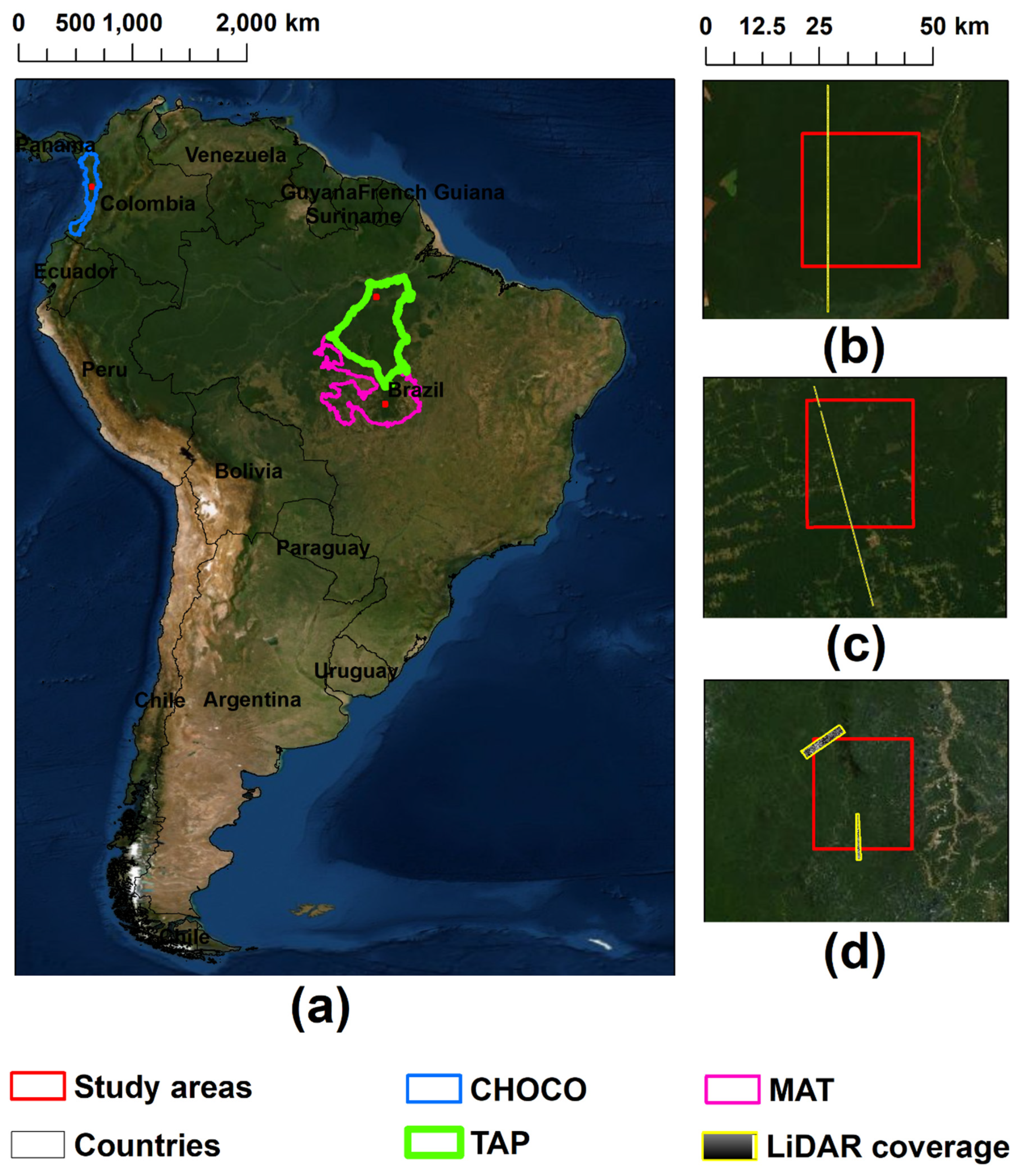
2.1. Study Areas and Forest Types

Since a rainfall regime is one of the main determinants of leaf phenology (greenness maximization) and microclimate in the tropical forests [51], we selected three locations in three types of tropical forest areas of South America with different annual rainfall totals (Figure 1): (1) Mato Grosso dry forest (MAT) is a transitional forest located in the Mato Grosso and Pará provinces of Central Brazil. MAT presents a high diversity of plants, animals and indigenous peoples. Average temperature is 23.5 °C and annual rainfall is around 2050 mm with eight moist months from December to May and four dry months from June to September [52]. The seasonal climatology in MAT is similar to the south American moist forests and savannas; however, this transitional forest typically receives about 200 mm less rainfall per year than the moist forests and 500 mm more rainfall than the savannas [53]. (2) Tapajós-Xingu moist forest (TAP) is located between the Tapajós and Xingu rivers that flow within the Amazon Basin of central-eastern Brazil. These forests host impressive levels of biodiversity and are characterized by a high density of lianas (woody vines), which creates a low and open understory. Average temperature is 25–28 °C, annual rainfall is around 2147 mm, and dry months are from August to October [54]. (3) Chocó-Darien rainforests (CHOCO) is located along the Colombian Pacific coast and the southeastern of Panama [55]. Past geologic events have turned this forest into one of the most diverse and endemic tropical forest areas on the Earth [56,57]. CHOCO is among the rainiest areas on the planet with an annual average rainfall between 8000 to 13000 mm and a lower rainfall season from January to March. The average temperature is 23 °C [58].

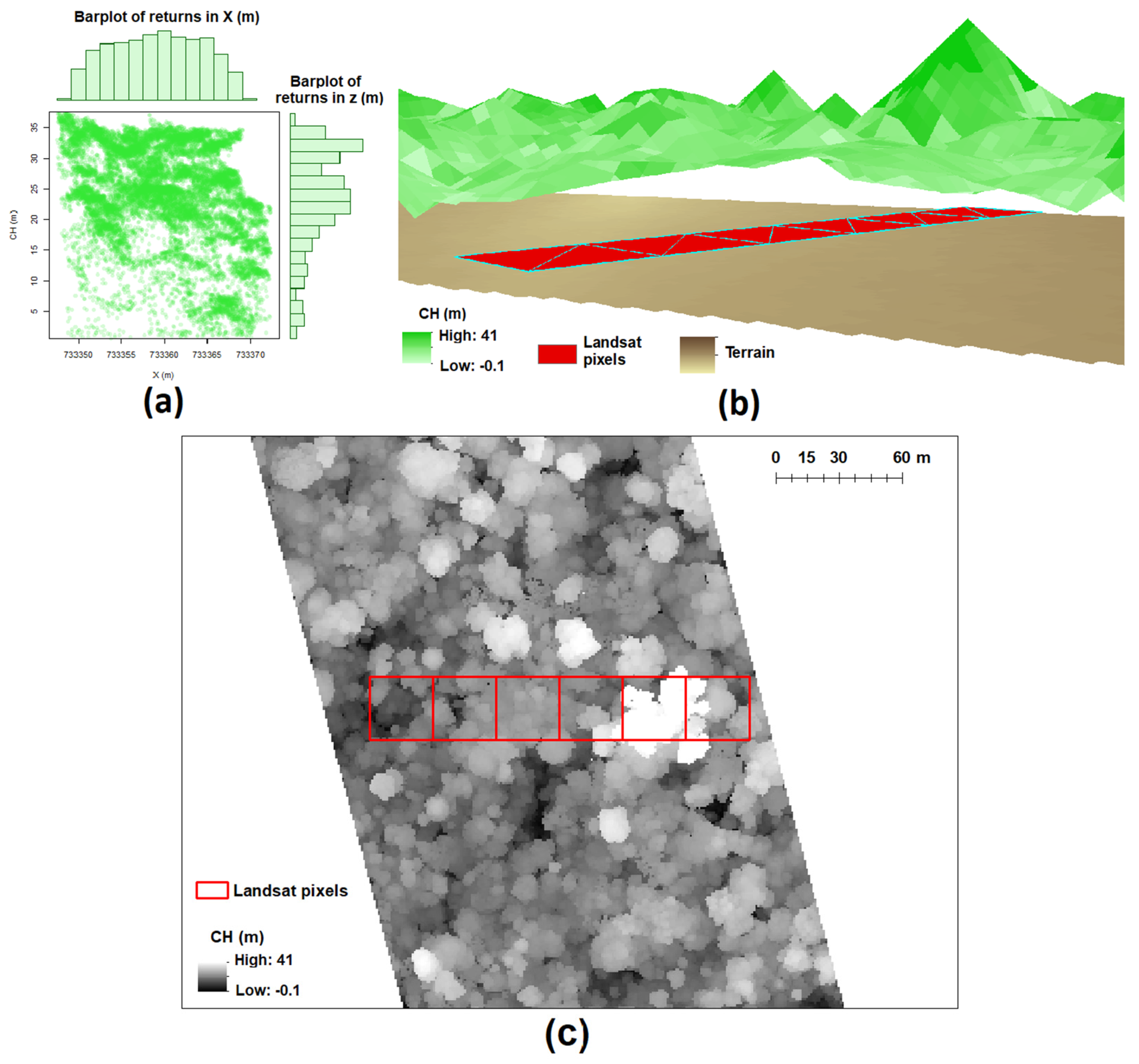
2.2. LiDAR Data and Canopy Height

Airborne discrete return LiDAR data were acquired during the dry months of 2018 for MAT and TAP by the Sustainable Landscapes Brazil project supported by the Brazilian Agricultural Research Corporation (EMBRAPA), the US Forest Service, USAID, and the US Department of State, using an OPTECH ALTM 3100 at an average flight altitude of 750 m with average return density of 22 returns/m2. For CHOCO, the LiDAR data were acquired using an OPTECH ALTM3033 during lower rainfall months of 2018 at an average flight altitude of 1000 m with average return density of 24 returns/m2. The LiDAR surveys were located in lowland, nonflooded areas of the three forest types at 44 m above sea level elevation average in MAT, 51 m in TAP, and 12 m in CHOCO. These data were processed by summing the returns within a laser footprint calculated at 1 m spatial resolution and 1-m vertical resolution [23,59]. Firstly, we selected the ground returns (Classification = 2 according to LAS file format) and generated 1-m DTMs (digital terrain models) using the k-nearest neighbor approach with the inverse-distance weighting (IDW). We then obtained normalized heights (heights above ground) for each point of the point cloud, subtracting the estimated ground elevation from the raw point elevation value. We then selected the highest reflections in the 1-m spatial resolution to compute 1-m CH models. Secondly, we calculated height percentile metrics at 98% of the cumulative points relative to the ground (Figure 2a). We used height metrics at 98% as estimation of the CH (Figure 2b); previous analyses have shown this height metric is the most precise canopy estimator since height metrics at 100% can be noisy due to its association with the first return [21]. The CHs of 1 m of spatial resolution (Figure 2c) were subsequently resampled at 30 m of spatial resolution using bilinear interpolation to align with 30 m Landsat-8 grids. These procedures were implemented using the R packages “Raster” and “lidR” [60,61].

2.3. Multispectral and SAR Data

We used data from three satellite instruments that observe different regions of the electromagnetic spectrum: (1) Four bands of the multispectral sensor Landsat-8: shorth wave infrared1 – SWIR1 (1.566–1.651 μm), short wave infrared2 – SWIR2 (2.107–2.294 μm), brightness temperature1 – Thermal1 (10.60–11.19 μm), and brightness temperature2 – Thermal2 (11.50–12.51 μm). In addition, we included the Enhanced Vegetation Index (EVI) and the Normalized Difference Vegetation Index (NDVI) estimated from Landasat-8. These indices detect complementary vegetation characteristics. EVI reduces atmospheric influence and is sensitive in denser canopies where NDVI tends to saturate; NDVI is better than EVI at detecting vegetation cover with low biomass and CH [62,63,64]. We did not use blue (0.452–0.512 μm), red (0.636–0.673 μm) and near infrared-NIR (0.851–0.879 μm) of Landasat-8 in our analysis since these bands are included in EVI and NDVI estimations. (2) The HV and HH polarization backscattering coefficients of the radar L-band generated by the SAR sensor ALOS-2-PALSAR (Phased Array type L-band Synthetic Aperture Radar). (3) The VV and VH polarization backscattering coefficients of the radar C-band generated by the SAR sensor Sentinel-1 (H refers to horizontal and V refers to vertical).
These data were obtained in Google Earth Engine [65]. For the Landsat data, we used the USGS Landsat-8 Surface Reflectance Tier-1 product. In this product, the visible bands, NIR, and SWIRs are processed to orthorectified surface reflectance while the two thermal bands (Thermal1 and Thermal2) are processed to orthorectified brightness temperature. These data are also atmospherically corrected using LaSRC (Landsat 8 Surface Reflectance algorithm), which includes cloud, shadow, water and snow masks [66]. These filters produced between seven and nine corrected values for each band per year in the study areas; we used these values to estimate annual means (X-means) and annual standard deviations (X-Sds) of the Landsat-8 data. All the Landsat bands are acquired at 30-m resolution, except the thermal bands that are resampled from 100 m to 30 m using cubic convolution to match the other spectral bands [67]. For the ALOS-2-PALSAR data, we used the Global PALSAR-2/PALSAR Yearly Mosaic [40]. This product has only one date per year; thus, we used three years (the previous, the actual, and the posterior years) to estimate X-means and X-Sds. The original spatial resolution of this product is 25 m; thus, it was resampled to the 30-m Landsat spatial resolution using bilinear interpolations. For the Sentinel-1 data, we used the product Sentinel-1 SAR GRD. This collection provides weekly data processed using the Sentinel-1 Toolbox to generate a calibrated and ortho-corrected product [68]. We estimated X-means and X-Sds using these weekly data. The original spatial resolution of this product is 15 m; therefore, we also resampled these data to the 30 m-Landsat spatial resolution using bilinear interpolations. We evaluated possible relations between the CHs of the LiDAR surveys and the X-means and X-Sds of these multispectral and SAR data using linear and nonlinear correlation analyses. We also used these X-means and X-Sds as the predictors of our models (see Modeling and Mapping). Our method for integrating discrete return LiDAR, Lansat-8, Sentinel-1, and PALSAR-2/PALSAR data was not a strict remote sensing fusion; we used the CHs estimated from LiDAR surveys as ground reference see [21,46,47] to model CHs to areas with not LiDAR coverage using annual metrics of the multispectral and SAR as predictors.
We estimated annual curves using only the corrected values for each band per year (multispectral and SAR data) at spatial resolution of 30 m in the areas corresponding to the LiDAR surveys. We applied a Gaussian filter with a temporal window of two corrected values in each annual curve for smoothing and improving its differentiation. The annual curves of each band were compared between lower CHs and upper CHs in the three forest types. Lower CHs were areas with vegetation canopy < 4 m while upper CHs were areas with vegetation canopy > 25 m in MAT and >30 m in TAP and CHOCO; the sizes of the upper CHs were different among forest types due to the availability of data. To build these annual curves, we first selected randomly 74 pixels for each of both CH classes in MAT, 100 pixels in TAP, and 69 in CHOCO. The number of evaluated pixels varied among the three study areas due to the availability of the data. We then averaged these curves across the CH classes, bands, and forest types and evaluated possible significant differences between the two CH classes per band in each study area using paired t-tests.

2.4. Modeling and Mapping
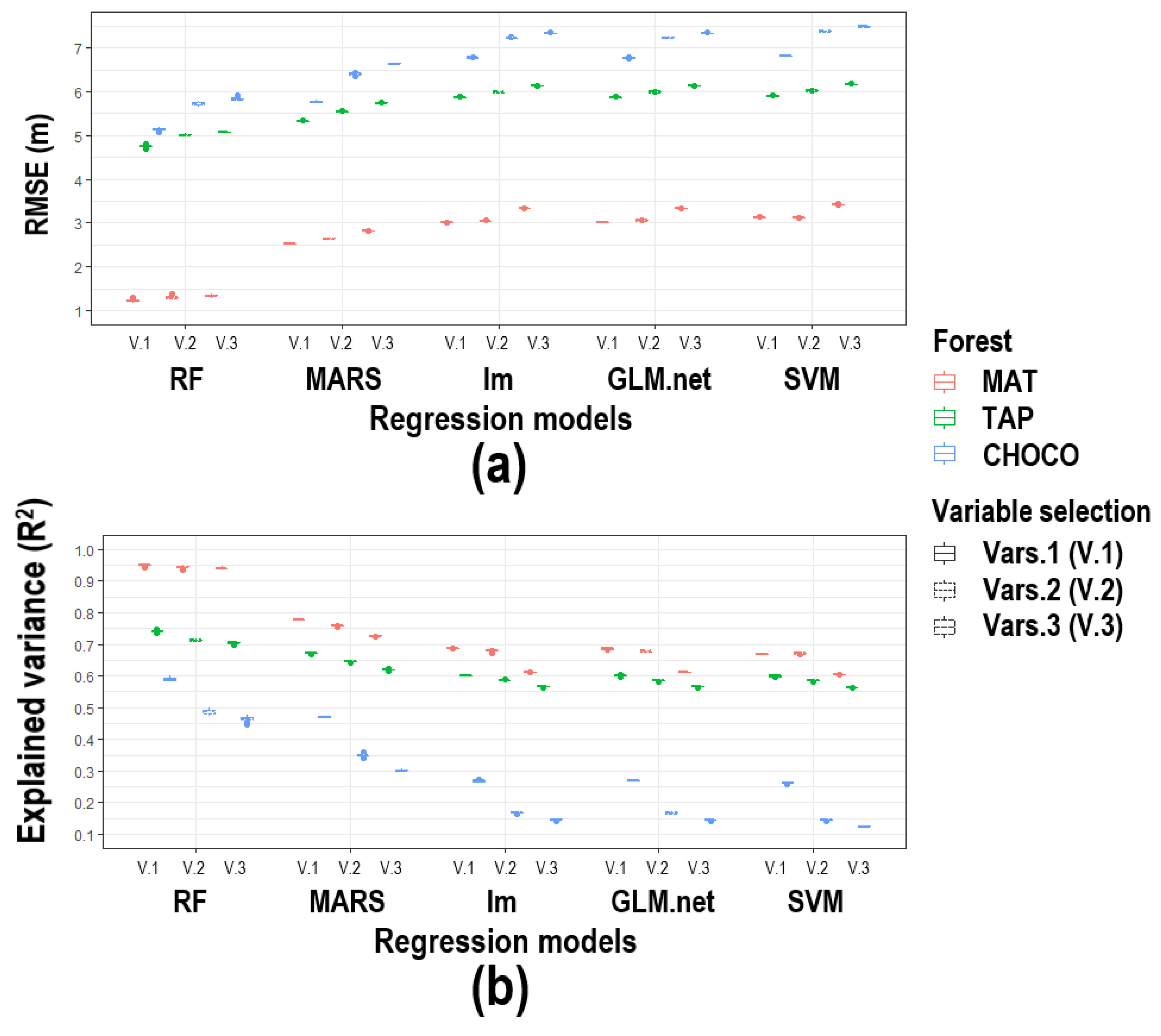
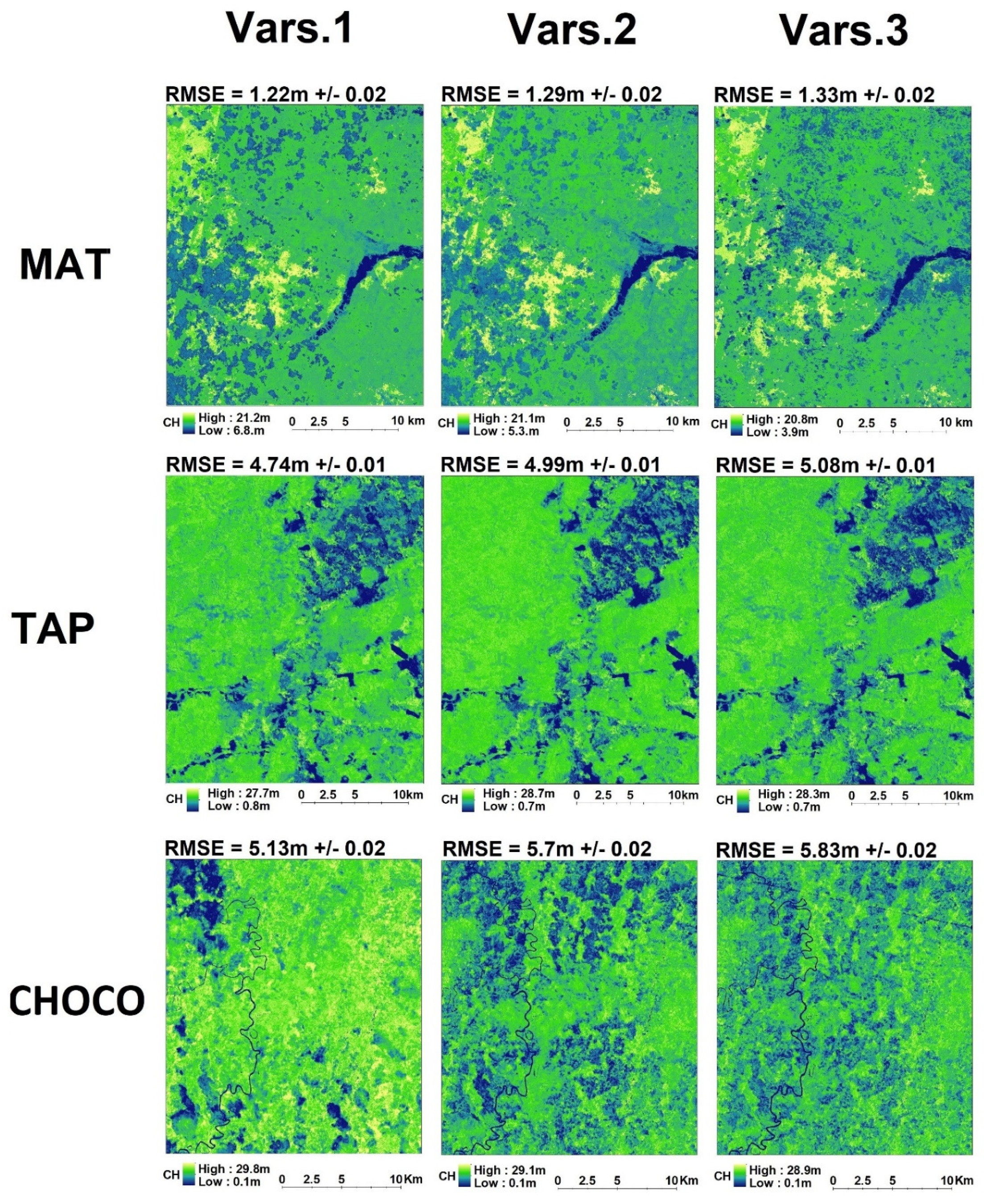
We used five different regression algorithms to model the relationship between LiDAR estimated CH and the X-means and X-Sds of the multispectral and SAR predictors—linear regression (lm), random forest (RF), support vector machine (SVM), multivariate adaptive regression splines (MARS), and Lasso and Elastic-Net Regularized Generalized Linear Models (GLM.net). We initially had 20 predictors; 10 X-means and 10 X-Sds corresponded to EVI, NDVI, SWIR1, SWIR2, Thermal1, Thermal2, L-band polarizations HV and HH, and C-band polarizations VV and VH. We grouped the variables in three different sets to run the five regression models. A first group formed by the 20 predictors variables (Vars.1). A second group of predictor variables (Vars.2) that included only the X-means and X-Sds with significant linear (significant r > 0.2) or nonlinear (significant k > 0.2) correlations to the CH in any of the three study areas since small r and k do not affect the trends of the response variables and could overfit the models [8]. We then examined the multicollinearity among the predictors with significant relations to the CH (r > 0.2), performing variance inflation factor through a stepwise procedure to eliminate correlated predictors and thus reduce possible overfitting effects in the regression models [69] using the R package “usdm” [70]. These predictor variables formed the third group (Vars.3).
We ran the five regression algorithms using 30-m pixel training sites where CH was estimated by the LiDAR surveys: 7408 training sites in MAT, 3207 in TAP, and ,024 in CHOCO (Table 1). The training sites were selected using a spatial filter of 60 m2 to reduce spatial autocorrelation. We used RMSE (root mean squared error) and MAE (mean absolute error) to evaluate the accuracy of the models. RMSE and MAE express average model prediction error in units of the variable of interest; however, RMSE gives a relatively high weight to larger errors and MAE penalizes greater variances of the errors [71]. We reported RMSE in the results and MAE in the Figure S1. We also estimated the explained variation or explained variance (adjusted R2) by the predictors in the models to evaluate the fit of the predictors (Vars.1, Vars.2, and Vars.3) in the models where higher adjusted R2 corresponds to better fit. We performed 100 iterations for each of the five regression models in the three study areas using the R Package “caret” [72]; each iteration included a fivefold cross-validation to estimate RMSE, MAE and adjusted R2. We performed stepwise model selections by AIC using the R packages “MASS” [73] for the lm regressions. For the RF regressions, we used 500 trees and three as the number of variables randomly sampled as candidates at each split of each tree; we used the R package “randomForest” [74]. For the SVM regressions, we performed linear kernels and used a value of one as the cost of constraint violation in the models; we used the R package “e1071” [75]. We used the R packages “earth” [76] and “glmnet” [77] and followed their default settings to implement the MARS and GLM.net regressions. MARS is an extension to linear regression that captures nonlinearities and interactions between variables [78] while GLM.net fits generalized linear model via penalized maximum likelihood [79]. Using these regression algorithms, we finally generated maps of the CH based on the multispectral and SAR predictors. The maps were create using the R package “raster” [60] and the spatial prediction (extent of maps) was less than 100 times the coverage of the LiDAR surveys [22]. In this work, we only present the maps generated by the most accurate regression model.

3. Results

Differences between annual curves of multispectral bands and vegetation indices were discernable in MAT and TAP when lower and upper CHs were compared (p < 0.05; t > 2.6); however, only the NDVI annual curves showed significant differences between both CH classes in CHOCO (p < 0.05; t > 3.6) (Table 2). SWIR1, SWR2, Thermal1 and Thermal2 were lower the whole year in upper CHs of MAT and during most of the year in upper CHs of TAP. In CHOCO, these four multispectral bands were similar in lower and upper CHs through most of the year (Figure 3). EVI and NDVI were higher through the whole year in upper CHs of MAT and during most of the year in upper CHs of TAP. Both vegetation indices also were similar most of the year in CHOCO (Figure 3). Differences between annual curves of both polarizations of the L-band were discernable between lower and upper CHs in MAT (p < 0.05), but differences were discernable only in the polarization HV in TAP (p < 0.3) and only the polarization HH in CHOCO. Annual curves of both polarizations of the C-band were discernable between lower and upper CHs in MAT and TAP, but only the VH polarization in CHOCO (p < 0.05) (Table 2).
All X-means of the bands and vegetation indices were linearly correlated to CH in MAT with r magnitudes > 0.2, eight of these variables in TAP, and six in CHOCO. The magnitudes of these linear correlations were higher in MAT, lower in TAP, and even lower in CHOCO for each vegetation index and band, except the C-band polarizations in CHOCO that were higher compared with TAP. X-means of the two SWIRs decreased with CH in the three forest types while EVI and NDVI increased. X-means of both thermal bands decreased with the CH in MAT and TAP but did not show significant trends in CHOCO. X-means of L-bands and C-bands increased with CH in the three forest types (Table 3, Figure S2). Four of the X-SDs were linearly correlated to CH in MAT with r magnitudes > 0.2, two of them in TAP, but none in CHOCO. These four X-SDs (EVI, NDVI, and the C-bands) decreased with the CH and their r magnitudes were higher in MAT than in TAP (Table 4, Figure S3). In general, the nonlinear coefficients of X-means and X-SDs for each vegetation index and band showed lower correlation magnitudes than the linear coefficients (Table 3 and Table 4).
A multifactorial ANOVA showed that the forest type (F = 47,764,132; p < 0.001; n = 4500), the regression algorithm (F = 2,933,759; p < 0.001; n = 4500), and the method of predictor variable selection (F = 488,825; p < 0.001; n = 4500) significantly affected the accuracy of the models for predicting CH (Figure 4a). By forest type, we found that the five regression models in each of the three methods of predictor selection resulted in the lowest RMSEs in MAT (2.6 m +/− 0.7 in average), intermedia RMSEs in TAP (5.7 m +/− 0.4 in average), and the highest RMSEs in CHOCO (6.6 m +/− 0.7 in average), showing that the prediction of CH are more accurate in the dry forest (MAT) (Figure 4a). By regression algorithm, RF regressions produced the lowest RMSEs in the three forest types (1.2 m +/− 0.05 in MAT, 4.9 m +/− 0.14 in TAP, and 5.5 m +/− 0.3 in CHOCO), MARS resulted in the second lowest RMSEs (2.6 m +/− 0.11 in MAT, 5.5 m +/− 0.17 in MAT, and 6.2 m +/− 0.36 in CHOCO), and the rest of regression algorithms (lm, GLM.net, and SVM) showed higher RMSEs (Figure 4a). By predictor variable selection, RMSEs were slightly lower for Vars.1 than for Vars.2 and Vars.3 in each regression set in MAT and TAP; these differences were lesser than 0.29 m in MAT and 0.26 m in TAP. However, the RMSEs are substantial lower for Vars.1 than Vars.2 and Vars.3 in CHOCO; these differences were higher than 0.6 m in general.
Another multifactorial ANOVA showed an analogous pattern for the explained variance; forest type (F = 21,615,347; p < 0.001; n = 4500), regression model (F = 2,999,577; p < 0.001; n = 4500), and method of predictor variable selection (F = 599,039; p < 0.001; n = 4500) affected significantly the explained variance of the models for predicting CH (Figure 4b). By forest type, the five regression models in the three methods of variable selection produced the highest average adjusted R2 in MAT (0.73 +/− 0.1 in average), intermediate adjusted R2 in TAP (0.62 +/− 0.05 in average), and the lowest adjusted R2 in CHOCO (0.29 +/− 0.14 in average), showing that predictors fitted better in the regressions corresponded to the dry forest (MAT). By regression model, RF regressions produced the highest adjusted R2 in the three forest types (0.94 +/− 0.01 in MAT, 0.72 +/− 0.01 in TAP, and 0.52 +/− 0.05 in CHOCO) and MARS resulted in the second highest adjusted R2 (0.75 +/− 0.2 in MAT, 0.64 +/− 0.2 in MAT, and 0.38 +/− 0.7 in CHOCO). For variable selection, the adjusted R2 tend to be slightly higher for Vars.1 than for Vars.2 and Vars.3 in each regression sets of MAT and TAP (differences lesser than 0.07 in general), but adjusted R2 was substantial higher in the regression sets of CHOCO (differences higher than 0.13 in general). Finally, the accuracies of CH-models using the best regression algorithm (RF) were higher in MAT (1.22 to 1.33 m) than in TAP (4.7 to 5 m) and CHO (5.13 to 5.83 m) (Figure 5).

4. Discussion

4.1. Improving CH Mapping

The first key contribution of our work was the use of annual metrics (X-means and X-SDs) of multispectral and SAR predictors for improving the mapping of CH LiDAR measures in tropical forests. Depending on forest type, our CH models reached errors close to 1 m and explained 94% of variance in CH, which are better than reported in previous work for tropical forests [36,42,47,80]. Because we used free and open resources (imagery and software), this improvement of the CH mapping can be adopted to facilitate the accurate long-term global monitoring of this EBV. Annual metrics of multispectral and SAR predictors also could be examined to model spatially other EBVs (such as the other ecosystem structure variables) using discrete or waveform LiDAR sensors as ground reference (including GEDI that is available from 2019) because both LiDAR technologies generate accurate measures of vegetation structure.
The improvement of the spatial estimation of CH is a result of the integration of two main factors: (1) The use of bands of different regions of the electromagnetic spectrum increased sensitivity to CH, likely due to forest characteristics such as leaf phenology, leaf density, moisture, and temperature; (2) The use of annual metrics reduced the errors produced when data of specific dates are used as we showed in our analysis of annual curves (Figure 3), where lower and upper CHs had similar band and vegetation indices values during some parts of the year while X-means were different. Other work has also demonstrated improved vegetation characterization when annual metrics of multispectral sensors are used, supporting our results [36,64,81,82].
We found the X-means of ten predictors (EVI, NDVI, two SWIRs, two thermal bands, two polarization of the L-band, and two polarization of the C-band) and four of their X-SDs (EVI, NDVI, and two polarization of the C-band) varied with CH, making them useful predictors of our CH map models and confirming ecological characteristics that have been researched previously. We specifically found that X-means of EVI and NDVI increased with the CH whereas their X-SDs decreased, suggesting variations of leaf phenology and leaf density related to CHs. Previous studies have found that a greenness maximization in well-preserved tropical forests (the areas of upper canopies in tropical forest) results in high and persistent yearly greenness [8,10,32]. Our results show that this greenness maximization is reduced in earlier succession (the areas of lower statured canopies in tropical forest), resulting in lower X-means and higher X-SDs of EVI and NDVI in these areas.
We also found negative correlations between the X-means of SWIR bands and CHs, indicating vegetation moisture changes with CH variations since the SWIRs of Landsat-8, specially SWIR2, are sensitive to water content of soil and vegetation [83]. The areas of upper CH in the well-preserved tropical forests are characterized by higher and more stable moisture during rainy and dry seasons. Conversely, areas of lower CH and biomasses or earlier succession (secondary vegetation and degraded forests) are more susceptible to incidence of light, air temperature change, and wind, which decreases the relative humidity in soil and litter, suggesting a mechanism for our results [13,14,84]. Other studies have identified similar gradients of moisture content using SWIRs in soils [85] or have inferred degrees of vegetation water stress and subsequent reduction of plant productivity [86,87], also supporting our results.
Our results show negative correlations between the X-means of thermal bands and the CH. Thermal band values are directly related to land surface temperature [88]; thus, our results show reductions of the land surface temperature with increasing CH. High evapotranspiration consumes more heat, decreasing the land surface temperature [89]. Evapotranspiration is higher in forest with high biomass compared with earlier successional forest [90]. These differences in evapotranspiration are consistent with our findings of cooler temperatures in taller forests. Using multispectral sensors, others have found land surface temperature is affect by land cover type and biophysical characteristics, such as elevation and aspect, at moderate to coarse spatial resolutions [91,92]. Our methods were able to detect differences in land surface temperature at moderately high spatial resolution in the same vegetation type, elevation, and aspect, confirming that annual metrics increase the ability of remote sensors to distinguish ecological characteristics in tropical forests.
X-means of the polarizations of the L-band were positively correlated with CH, which is consistent with previous studies showing the backscatter of SAR sensors can be used for estimation of CH [38,93]. Until P-band spaceborne SAR data, which is able to more deeply penetrate forest canopies, becomes available from the ESA BIOMASS Mission, L-band is the most suitable operational spaceborne SAR data for estimation of forest structure variables [94]. The X-means of the C-band also increased with CH. Although the C-band is not able to deeply penetrate forest canopies, the higher backscatter of both C-band polarizations in upper CHs is consistent with high densities of leaves in the upper canopies. Emergent tall trees and lianas compete for light in the well-preserved forest producing dense canopy strata [95] and generating the high values for the C-band backscatter captured in our analyses. Leaf density is lower in earlier succession, consistent with lower C-band backscatter.

4.2. Map Accuracy Among Forest Types

The second key contribution of our work was demonstrating that the accuracy of the CH maps in tropical forests decrease from dry forests to moist and rainforests. Variations of our analyses, which were generated by different remote sensing resources and methods, each supported this finding. All our model combinations using five regression algorithms and three selections of predictor variables produced the highest accuracies and explained variations in the dry forest (MAT), were lower in the moist forest (TAP), and were even lower in the rainforest (CHOCO). These patterns were generated due to the reduction of predictors correlated with CH and the decreasing magnitude of these correlations in moist and rainforest. A lower quality of the multispectral sensor data in moist and rainforests could explain the general decline of these correlations since these forests present high levels of aerosol gases and clouds that attenuate multispectral imagery [64]. Our multispectral predictors were likely to be slightly less affected by aerosol gases and clouds since we used annual series formed by two-month mosaics of Landsat-8 using CFMask (The C Function of Mask) filters (i.e., filters for selecting pixels with low aerosol gases and no-clouds). Additionally, correlations between SAR predictors and CH also decreased in the moist and rainforest, despite the fact that C- and L-band SAR data are not substantially affected by aerosol gases and clouds. Thus, changes of ecological characteristics from the dry forest to the moist and rainforest would be the main cause of the general declining of these correlations and their subsequent effects in the accuracy of our CH maps and models.
We found higher magnitudes of the correlations in the dry forest, indicating that early succession (lower CHs) and late succession (upper CHs) in dry forest areas present higher ecological contrasts than early and late succession in moist and rainforest areas. Others have confirmed that environmental conditions are more restrictive for vegetation regeneration in dry forests than in moist and rainforests, such as lower rainfalls, higher temperatures, intense light incidences, and stronger winds, supporting our results [96,97]. Stronger negative correlations between thermal bands and CHs in the dry forest confirm lesser growth, biomass, and evapotranspiration [98], resulting in higher contrast of land surface temperatures between upper and lower CHs compare with moist and rainforests. We also found lower and upper CHs had different values of SWIRs, EVI and NDVI in the dry forest through the year whereas they were similar most of the year in the rainforest areas. High rainfall in the rainforest (>8000 mm) throughout the year generates high moisture levels and leaf densities across stages of forest succession, including stages with low CHs. Thus, SWIRs, EVI, and NDVI can show similar values in different CHs of CHOCO, reducing the magnitude of their correlation to the CH. Conversely, the lower rainfall in the dry forest (2050 mm) with four dry months in the year generates lower moisture levels and higher leaf deciduousness during dry season, affecting lower CHs more strongly. Hence, SWIRs, EVI, and NDVI show lower values in the lower CHs, increasing the magnitude of their correlation with CH.

4.3. Map Accuracy Among Predictor Sets

The final key contribution of our work was showing possible overfitting effects when multispectral and SAR predictors are used to build CH maps. In the three tropical forest types using five different regression algorithms, our results showed differences in the accuracy of the CH map models agree with three sets of predictor variables. The best classification accuracies and explained variances were generated by a set of 20 multispectral and SAR predictors (ten X-means and ten X-SDs), including six predictors that did not show linear or nonlinear correlations to CH. When these six predictors were eliminated, the CH map model accuracies and explained variances decreased slightly in the dry forest (+/−0.1 m and −1%) and moist forest (+/−0.2 m and −2%) but considerably in the rainforest (+/−0.5 m and −11%), showing a higher effect of the accumulation of predictors in the accuracy estimation where the relationship between CH and predictors presented the highest uncertainty, suggesting a higher susceptibility to overfitting in this set of predictors [99]. We then eliminated collinear predictors, resulting in another slight decrease of the accuracies and explained variances in the dry forest and moist forest compares with a substantial decrease of the rainforest, showing again higher possible effects of overfitting in the rainforest by the accumulation of predictors. The previous examinations have confirmed the high susceptibility of remote sensing analyses to overfit their training set data [100].
The RF regressions produced the best accuracies and explained variances than the other regressions algorithms. Others have also found RF models are more accurate than other machine learning algorithms in remote sensing analyses [101,102]. Interesting, we also found that the accuracies produced by RF regressions were less affected by the changes of predictor sets than the other four regression algorithms. Observed accuracy did not differ substantially among the three predictor sets in the dry forest and changed only slightly in the moist forest. This lower susceptibility to overfitting would be another factor indicating RF has advantages over other learning algorithms in remote sensing analysis.

5. Conclusions

The accuracy of canopy height mapping using LiDAR surveys as reference sample can be improved by integrating multispectral and SAR band predictors. Each band’s reflectance or backscatter is related to different forest ecological characteristics that vary with changes in canopy height, producing differential relations between canopy height and each band reflectance or SAR backscatter. Likewise, annual metrics improve the relationship between canopy height and our predictor variables, resulting in more accurate mapping of canopy height in tropical forests. We found the accuracy of canopy height maps produced from our analyses decreased from dry forest to moist and rainforest, likely a result of more structurally complex canopies presenting less annual and interannual variability due to effective partitioning of light and water resources at different canopy levels. Consequently, uncertainty and overfitting of canopy height is more difficult to constrain over rainforest areas. Although we did not model potential effects of the GEDI mission’s spatial sampling approach, we processed our airborne discrete return LiDAR data to a similar spatial resolution (30 m). Thus, our results have relevance to improving the prediction and mapping of canopy height using this new data source that will be available in the near future and increase through time. Overall, our results suggest that metrics derived from multispectral and SAR imaging sensors will allow development of more accurate maps of canopy height and other forest structural variables across a range of forest types while GEDI data will allow the generality of these results to be tested on a much wider array of forest types than what is currently feasible with limited aircraft LiDAR coverage. The measure of other forest traits could be also improved by integrating annual metrics of multispectral and SAR bands, such as forest degradation, diversity, and phenology. We have interpolated the response and predictor and predictor variables to the spatial resolution of 30 m, the lowest spatial resolution among these variables. Thus, the estimation of canopy height and other forest traits could be improved by integrating annual metrics of remote sensors with higher spatial, spectral, and temporal resolution, such as the multispectral sensor Sentinel-2.

Supplementary Materials

The following are available online at https://www.mdpi.com/2072-4292/11/22/2697/s1, Figure S1: Accuracy of the map models estimated as MAE (Mean Absolute Error) in three tropical forests, Figure S2: Linear and nonlinear correlations between canopy height (CH) and X-means of multispectral and SAR predictors in three tropical forest, Figure S3: Linear and nonlinear correlations between canopy height (CH) and X-SDs of multispectral and SAR predictors in three tropical forest.

Author Contributions

Conceptualization, J.C.F., P.J. and S.J.G.; Methodology, J.C.F. and P.J.; Formal analysis, and Sassan Saatchi and the Jet Propulsion Laboratory of NASA for providing LiDAR data. and P.J.; Investigation, J.C.F., P.J. and S.J.G.; Resources, P.J. and S.J.G.; Writing—review & editing, J.C.F., P.J., S.R.-B., L.D. and S.J.G.

Funding

This research was funded by the National Aeronautics and Space Administration, NASA GEO - grant number 2017-2020.

Acknowledgments

We acknowledge NASA GEO for supporting this research, GEODE Lab of the School of Informatics, Computing, and Cyber Systems (SICCS) at Northern Arizona University for providing additional financial and technical support, Instituto Humboldt of Colombia for technical support, and Sassan Saatchi and the Jet Propulsion Laboratory of NASA for providing LiDAR data. This work is one of requirements for the forgiveness of the COLCIENCIAS-loan 529-2011 for J.C.F.

Conflicts of Interest

We declare no conflict of interest for any part of this manuscript. We also confirm that neither the manuscript nor any parts of its content are currently under consideration or published in another journal.

References

  1. Pereira, H.M.; Ferrier, S.; Walters, M.; Geller, G.N.; Jongman, R.H.G.; Scholes, R.J.; Bruford, M.W.; Brummitt, N.; Butchart, S.H.M.; Cardoso, A.C.; et al. Essential biodiversity variables. Science 2013, 339, 277–278. [Google Scholar] [CrossRef] [PubMed]
  2. Skidmore, A.K.; Pettorelli, N.; Coops, N.C.; Geller, G.N.; Hansen, M.; Lucas, R.; Muecher, C.A.; O’Connor, B.; Paganini, M.; Pereira, H.M.; et al. Agree on biodiversity metrics to track from space. Nature 2015, 523, 403–405. [Google Scholar] [CrossRef] [PubMed]
  3. Vihervaara, P.; Auvinen, A.-P.; Mononen, L.; Törmä, M.; Ahlroth, P.; Anttila, S.; Böttcher, K.; Forsius, M.; Heino, J.; Heliölä, J.; et al. How essential biodiversity variables and remote sensing can help national biodiversity monitoring. Glob. Ecol. Conserv. 2017, 10, 43–59. [Google Scholar] [CrossRef]
  4. Primack, R.B.; Corlett, R.T. Tropical Rain Forests: An Ecological and Biogeographical Comparison; Blackwell Publishing: Oxford, UK, 2009; ISBN 978-1-4051-4109-3. [Google Scholar]
  5. Hubbell, S.P.; Foster, R.B.; O’Brien, S.T.; Harms, K.E.; Condit, R.; Wechsler, B.; Wright, S.J.; de Lao, S.L. Light-gap disturbances, recruitment limitation, and tree diversity in a neotropical forest. Science 1999, 283, 554–557. [Google Scholar] [CrossRef]
  6. Kellner, J.R.; Clark, D.B.; Hubbell, S.P. Pervasive canopy dynamics produce short-term stability in a tropical rain forest landscape. Ecol. Lett. 2009, 12, 155–164. [Google Scholar] [CrossRef]
  7. Clark, D.B.; Olivas, P.C.; Oberbauer, S.F.; Clark, D.A.; Ryan, M.G. First direct landscape-scale measurement of tropical rain forest Leaf Area Index, a key driver of global primary productivity. Ecol. Lett. 2008, 11, 163–172. [Google Scholar] [CrossRef]
  8. Smith, M.N.; Stark, S.C.; Taylor, T.C.; Ferreira, M.L.; de Oliveira, E.; Restrepo-Coupe, N.; Chen, S.; Woodcock, T.; dos Santos, D.B.; Alves, L.F.; et al. Seasonal and drought-related changes in leaf area profiles depend on height and light environment in an Amazon forest. NEW Phytol. 2019, 222, 1284–1297. [Google Scholar] [CrossRef]
  9. LaFrankie, J.V.; Ashton, P.S.; Chuyong, G.B.; Co, L.; Condit, R.; Davies, S.J.; Foster, R.; Hubbell, S.P.; Kenfack, D.; Lagunzad, D.; et al. Contrasting structure and composition of the understory in species-rich tropical rain forests. Ecology 2006, 87, 2298–2305. [Google Scholar] [CrossRef]
  10. Tang, H.; Dubayah, R. Light-driven growth in Amazon evergreen forests explained by seasonal variations of vertical canopy structure. Proc. Natl. Acad. Sci. USA 2017, 114, 2640–2644. [Google Scholar] [CrossRef]
  11. Wu, J.; Albert, L.P.; Lopes, A.P.; Restrepo-Coupe, N.; Hayek, M.; Wiedemann, K.T.; Guan, K.; Stark, S.C.; Christoffersen, B.; Prohaska, N.; et al. Leaf development and demography explain photosynthetic seasonality in Amazon evergreen forests. Science 2016, 351, 972–976. [Google Scholar] [CrossRef]
  12. De Frenne, P.; Zellweger, F.; Rodriguez-Sanchez, F.; Scheffers, B.R.; Hylander, K.; Luoto, M.; Vellend, M.; Verheyen, K.; Lenoir, J. Global buffering of temperatures under forest canopies. Nat. Ecol. Evol. 2019, 3, 744–749. [Google Scholar] [CrossRef] [PubMed]
  13. Sanchez, U.; Nino, S.; Barrientoso, L.; Trevino, J.; Almaguer, P. Seasonal microclimatic variation in a succession gradient of low thorn forest in Northeastern Mexico. Rev. Biol. Trop. 2019, 67, 266–277. [Google Scholar]
  14. Jucker, T.; Hardwick, S.R.; Both, S.; Elias, D.M.O.; Ewers, R.M.; Milodowski, D.T.; Swinfield, T.; Coomes, D.A. Canopy structure and topography jointly constrain the microclimate of human-modified tropical landscapes. Glob. Chang. Biol. 2018, 24, 5243–5258. [Google Scholar] [CrossRef]
  15. Hadi; Pfeifer, M.; Korhonen, L.; Wheeler, C.; Rautiainen, M. Forest canopy structure and reflectance in humid tropical Borneo: A physically-based interpretation using spectral invariants. Remote Sens. Environ. 2017, 201, 314–330. [Google Scholar] [CrossRef]
  16. Drake, J.B.; Knox, R.G.; Dubayah, R.O.; Clark, D.B.; Condit, R.; Blair, J.B.; Hofton, M. Above-ground biomass estimation in closed canopy Neotropical forests using lidar remote sensing: Factors affecting the generality of relationships. Glob. Ecol. Biogeogr. 2003, 12, 147–159. [Google Scholar] [CrossRef]
  17. Goetz, S.; Dubayah, R. Advances in remote sensing technology and implications for measuring and monitoring forest carbon stocks and change. CARBON Manag. 2011, 2, 231–244. [Google Scholar] [CrossRef]
  18. Guan, H.; Li, J.; Yu, Y.; Zhong, L.; Ji, Z. DEM generation from lidar data in wooded mountain areas by cross-section-plane analysis. Int. J. Remote Sens. 2014, 35, 927–948. [Google Scholar] [CrossRef]
  19. McRoberts, R.E.; Chen, Q.; Gormanson, D.D.; Walters, B.F. The shelf-life of airborne laser scanning data for enhancing forest inventory inferences. Remote Sens. Environ. 2018, 206, 254–259. [Google Scholar] [CrossRef]
  20. Huang, W.; Dolan, K.; Swatantrad, A.; Johnson, K.; Tang, H.; O’Neil-Dunne, J.; Dubayah, R.; Hurtt, G. High-resolution mapping of aboveground biomass for forest carbon monitoring system in the Tri-State region of Maryland, Pennsylvania and Delaware, USA. Environ. Res. Lett. 2019, 14, 1–16. [Google Scholar] [CrossRef]
  21. Silva, C.A.; Saatchi, S.; Garcia, M.; Labriere, N.; Klauberg, C.; Ferraz, A.; Meyer, V.; Jeffery, K.J.; Abernethy, K.; White, L.; et al. Comparison of small-and large-footprint lidar characterization of tropical forest aboveground structure and biomass: A case study from central gabon. IEEE J. Sel. Top. Appl. EARTH Obs. Remote Sens. 2018, 11, 3512–3526. [Google Scholar] [CrossRef]
  22. Asner, G.P.; Powell, G.V.N.; Mascaro, J.; Knapp, D.E.; Clark, J.K.; Jacobson, J.; Kennedy-Bowdoin, T.; Balaji, A.; Paez-Acosta, G.; Victoria, E.; et al. High-resolution forest carbon stocks and emissions in the Amazon. Proc. Natl. Acad. Sci. USA 2010, 107, 16738–16742. [Google Scholar] [CrossRef] [PubMed]
  23. Dubayah, R.O.; Sheldon, S.L.; Clark, D.B.; Hofton, M.A.; Blair, J.B.; Hurtt, G.C.; Chazdon, R.L. Estimation of tropical forest height and biomass dynamics using lidar remote sensing at La Selva, Costa Rica. J. Geophys. Res. 2010, 115, 1–17. [Google Scholar] [CrossRef]
  24. Tang, H.; Song, X.-P.; Zhao, F.A.; Strahler, A.H.; Schaaf, C.L.; Goetz, S.; Huang, C.; Hansen, M.C.; Dubayah, R. Definition and measurement of tree cover: A comparative analysis of field-, lidar-and landsat-based tree cover estimations in the Sierra national forests, USA. Agric. For. Meteorol. 2019, 268, 258–268. [Google Scholar] [CrossRef]
  25. Blair, J.B.; Hofton, M.A. Modeling laser altimeter return waveforms over complex vegetation using high-resolution elevation data. Geophys. Res. Lett. 1999, 26, 2509–2512. [Google Scholar] [CrossRef]
  26. Hancock, S.; Armston, J.; Hofton, M.; Sun, X.; Tang, H.; Duncanson, L.I.; Kellner, J.R.; Dubayah, R. The GEDI Simulator: A Large-footprint waveform lidar simulator for calibration and validation of spaceborne missions. EARTH Space Sci. 2019, 6, 294–310. [Google Scholar] [CrossRef] [PubMed]
  27. Popescu, S.C.; Zhao, K.; Neuenschwander, A.; Lin, C. Satellite lidar vs. small footprint airborne lidar: Comparing the accuracy of aboveground biomass estimates and forest structure metrics at footprint level. Remote Sens. Environ. 2011, 115, 2786–2797. [Google Scholar] [CrossRef]
  28. Bi, J.; Knyazikhin, Y.; Choi, S.; Park, T.; Barichivich, J.; Ciais, P.; Fu, R.; Ganguly, S.; Hall, F.; Hilker, T.; et al. Sunlight mediated seasonality in canopy structure and photosynthetic activity of Amazonian rainforests. Environ. Res. Lett. 2015, 10, 064014. [Google Scholar] [CrossRef]
  29. Doughty, C.E.; Goulden, M.L. Seasonal patterns of tropical forest leaf area index and CO2 exchange. J. Geophys. Res. 2008, 113, 1–12. [Google Scholar] [CrossRef]
  30. Rappaport, D.I.; Morton, D.C.; Longo, M.; Keller, M.; Dubayah, R.; dos-Santos, M.N. Quantifying long-term changes in carbon stocks and forest structure from Amazon forest degradation. Environ. Res. Lett. 2018, 13, 065013. [Google Scholar] [CrossRef]
  31. Huete, A.; Didan, K.; Miura, T.; Rodriguez, E.P.; Gao, X.; Ferreira, L.G. Overview of the radiometric and biophysical performance of the MODIS vegetation indices. Remote Sens. Environ. 2002, 83, 195–213. [Google Scholar] [CrossRef]
  32. Brando, P.M.; Goetz, S.J.; Baccini, A.; Nepstad, D.C.; Beck, P.S.A.; Christman, M.C. Seasonal and interannual variability of climate and vegetation indices across the Amazon. Proc. Natl. Acad. Sci. USA 2010, 107, 14685–14690. [Google Scholar] [CrossRef] [PubMed]
  33. Tang, H.; Armston, J.; Hancock, S.; Marselis, S.; Goetz, S.; Dubayah, R. Characterizing global forest canopy cover distribution using spaceborne lidar. Remote Sens. Environ. 2019, 231, 111262. [Google Scholar] [CrossRef]
  34. Brown, L.; Chen, J.M.; Leblanc, S.G.; Cihlar, J. A shortwave infrared modification to the simple ratio for LAI retrieval in boreal forests: An image and model analysis. Remote Sens. Environ. 2000, 71, 16–25. [Google Scholar] [CrossRef]
  35. Meyer, V.; Saatchi, S.; Ferraz, A.; Xu, L.; Duque, A.; Garcia, M.; Chave, J. Forest degradation and biomass loss along the Choco region of Colombia. Carbon Balance Manag. 2019, 14, 2. [Google Scholar] [CrossRef]
  36. Hansen, M.C.; Potapov, P.V.; Goetz, S.J.; Turubanova, S.; Tyukavina, A.; Krylov, A.; Kommareddy, A.; Egorov, A. Mapping tree height distributions in Sub-Saharan Africa using Landsat 7 and 8 data. Remote Sens. Environ. 2016, 185, 221–232. [Google Scholar] [CrossRef] [Green Version]
  37. Cartus, O.; Santoro, M.; Kellndorfer, J. Mapping forest aboveground biomass in the Northeastern United States with ALOS PALSAR dual-polarization L-band. Remote Sens. Environ. 2012, 124, 466–478. [Google Scholar] [CrossRef]
  38. Berninger, A.; Lohberger, S.; Staengel, M.; Siegert, F. SAR-based estimation of above-ground biomass and its changes in tropical forests of kalimantan using L- and C-Band. Remote Sens. 2018, 10, 831. [Google Scholar] [CrossRef] [Green Version]
  39. Saatchi, S.; Moghaddam, M. Estimation of crown and stem water content and biomass of boreal forest using polarimetric SAR imagery. IEEE Trans. Geosci. Remote Sens. 2000, 38, 697–709. [Google Scholar] [CrossRef] [Green Version]
  40. Shimada, M.; Itoh, T.; Motooka, T.; Watanabe, M.; Shiraishi, T.; Thapa, R.; Lucas, R. New global forest/non-forest maps from ALOS PALSAR data (2007–2010). Remote Sens. Environ. 2014, 155, 13–31. [Google Scholar] [CrossRef]
  41. Saatchi, S.; Marlier, M.; Chazdon, R.L.; Clark, D.B.; Russell, A.E. Impact of spatial variability of tropical forest structure on radar estimation of aboveground biomass. Remote Sens. Environ. 2011, 115, 2836–2849. [Google Scholar] [CrossRef]
  42. Urbazaev, M.; Cremer, F.; Migliavacca, M.; Reichstein, M.; Schmullius, C.; Thiel, C. Potential of multi-temporal ALOS-2 PALSAR-2 ScanSAR data for vegetation height estimation in tropical forests of Mexico. Remote Sens. 2018, 10, 1277. [Google Scholar] [CrossRef] [Green Version]
  43. Luckman, A.; Baker, J.; Honzák, M.; Lucas, R. Tropical forest biomass density estimation using JERS-1 SAR: Seasonal variation, confidence limits, and application to image mosaics. Remote Sens. Environ. 1998, 63, 126–139. [Google Scholar] [CrossRef]
  44. Saatchi, S.; Harris, N.L.; Brown, S.; Lefsky, M.; Mitchard, E.T.A.; Salas, W.; Zutta, B.R.; Buermann, W.; Lewis, S.L.; Hagen, S.; et al. Benchmark map of forest carbon stocks in tropical regions across three continents. Proc. Natl. Acad. Sci. USA 2011, 108, 9899–9904. [Google Scholar] [CrossRef] [PubMed] [Green Version]
  45. Kugler, F.; Schulze, D.; Hajnsek, I.; Pretzsch, H.; Papathanassiou, K.P. TanDEM-X Pol-InSAR performance for forest height estimation. IEEE Trans. Geosci. Remote Sens. 2014, 52, 6404–6422. [Google Scholar] [CrossRef]
  46. Qi, W.; Dubayah, R.O. Combining Tandem-X InSAR and simulated GEDI lidar observations for forest structure mapping. Remote Sens. Environ. 2016, 187, 253–266. [Google Scholar] [CrossRef]
  47. Qi, W.; Lee, S.-K.; Hancock, S.; Luthcke, S.; Tang, H.; Armston, J.; Dubayah, R. Improved forest height estimation by fusion of simulated GEDI Lidar data and TanDEM-X InSAR data. Remote Sens. Environ. 2019, 221, 621–634. [Google Scholar] [CrossRef] [Green Version]
  48. Bae, S.; Levick, S.R.; Heidrich, L.; Magdon, P.; Leutner, B.F.; Woellauer, S.; Serebryanyk, A.; Nauss, T.; Krzystek, P.; Gossner, M.M.; et al. Radar vision in the mapping of forest biodiversity from space. Nat. Commun. 2019, 10, 1–10. [Google Scholar] [CrossRef]
  49. Cartus, O.; Santoro, M.; Wegmuller, U.; Rommen, B. Benchmarking the retrieval of biomass in boreal forests using P-Band SAR backscatter with multi-temporal C- and L-Band observations. Remote Sens. 2019, 11, 1695. [Google Scholar] [CrossRef] [Green Version]
  50. Pham, T.D.; Yoshino, K.; Le, N.N.; Bui, D.T. Estimating aboveground biomass of a mangrove plantation on the Northern coast of Vietnam using machine learning techniques with an integration of ALOS-2 PALSAR-2 and Sentinel-2A data. Int. J. Remote Sens. 2018, 39, 7761–7788. [Google Scholar] [CrossRef]
  51. Abernethy, K.; Bush, E.R.; Forget, P.-M.; Mendoza, I.; Morellato, L.P.C. Current issues in tropical phenology: A synthesis. Biotropica 2018, 50, 477–482. [Google Scholar] [CrossRef] [Green Version]
  52. WWF. Mato Grosso Dry Forest. Available online: https://www.worldwildlife.org/ecoregions/nt0140 (accessed on 1 August 2018).
  53. Vourlitis, G.L.; Priante, N.; Hayashi, M.M.S.; Nogueira, J.D.; Caseiro, F.T.; Campelo, J.H. Seasonal variations in the evapotranspiration of a transitional tropical forest of Mato Grosso, Brazil. WATER Resour. Res. 2002, 38, 30-1–30-11. [Google Scholar] [CrossRef]
  54. WWF. Tapajós-Xingu Moist Forest. Available online: https://www.worldwildlife.org/ecoregions/nt0168 (accessed on 1 August 2018).
  55. WWF. Choco-Darien Moist Forests. Available online: http://wwf.panda.org/about_our_earth/ecoregions/chocodarien_moist_forests.cfm (accessed on 1 August 2018).
  56. Gentry, A.H. Species richness and floristic composition of Choco Region plant communities. Caldasia 1986, 15, 5. [Google Scholar]
  57. Gregory-Wodzicki, K.M. Uplift history of the central and northern Andes: A review. Geol. Soc. Am. Bull. 2000, 7, 14. [Google Scholar] [CrossRef]
  58. Poveda, G.; Mesa, O.J. On the existence of Lloro (the rainiest locality on earth): Enhanced ocean-land-atmosphere interaction by a low-level jet. Geophys. Res. Lett. 2000, 27, 1675–1678. [Google Scholar] [CrossRef] [Green Version]
  59. Clark, M.L.; Roberts, D.A.; Ewel, J.J.; Clark, D.B. Estimation of tropical rain forest aboveground biomass with small-footprint lidar and hyperspectral sensors. Remote Sens. Environ. 2011, 115, 2931–2942. [Google Scholar] [CrossRef]
  60. Hijmans, R.; van Etten, J.; Cheng, J.; Mattiuzzi, M.; Sumner, M.; Greenberg, J.; Perpinan, O.; Bevan, A.; Racine, E.; Shortridge, A. Package ‘Raster’: Geographic Data Analysis and Modeling. Package ‘Raster’. 2016. Available online: https://www.r-project.org/ (accessed on 1 August 2018).
  61. Roussel, J.-R.; David, A.; De Boissieu, F.; Meador, A.S. Package ‘lidR’: Airborne LiDAR Data Manipulation and Visualization for Forestry Applications. Package ‘lidR’. 2019. Available online: https://www.r-project.org/ (accessed on 1 August 2018).
  62. Huete, A.R.; Justice, C.; Leeuwen, W. MODIS Vegetation Index, Algorithm Theoretical Basis Document; University of Arizona and University of Virginia: Tucson, AZ, USA, 1999. [Google Scholar]
  63. Li, Z.; Li, X.; Wei, D.; Xu, X.; Wang, H. An assessment of correlation on MODIS-NDVI and EVI with natural vegetation coverage in Northern Hebei Province, China. Procedia Environ. Sci. 2010, 2, 964–969. [Google Scholar] [CrossRef] [Green Version]
  64. Fagua, J.C.; Ramsey, R.D. Geospatial modeling of land cover change in the Chocó-Darien global ecoregion of South America; one of most biodiverse and rainy areas in the world. PLoS ONE 2019, 14, e0211324. [Google Scholar] [CrossRef]
  65. Gorelick, N.; Hancher, M.; Dixon, M.; Ilyushchenko, S.; Thau, D.; Moore, R. Google earth engine: Planetary-scale geospatial analysis for everyone. Remote Sens. Environ. 2017, 202, 18–27. [Google Scholar] [CrossRef]
  66. USGS, U.G.S. USGS Landsat 8 Surface Reflectance Tier 1. Available online: https://developers.google.com/earth-engine/datasets/catalog/LANDSAT_LC08_C01_T1_SR (accessed on 1 August 2018).
  67. Anderson, M.C.; Allen, R.G.; Morse, A.; Kustas, W.P. Use of Landsat thermal imagery in monitoring evapotranspiration and managing water resources. Remote Sens. Environ. 2012, 122, 50–65. [Google Scholar] [CrossRef]
  68. ESA, E.S.A. Sentinel-1 SAR GRD: C-band Synthetic Aperture Radar Ground Range Detected, Log Scaling. Available online: https://developers.google.com/earth-engine/datasets/catalog/COPERNICUS_S1_GRD (accessed on 1 August 2018).
  69. Dormann, C.F.; Elith, J.; Bacher, S.; Buchmann, C.; Carl, G.; Carre, G.; Garcia Marquez, J.R.; Gruber, B.; Lafourcade, B.; Leitao, P.J.; et al. Collinearity: A review of methods to deal with it and a simulation study evaluating their performance. Ecography 2013, 36, 27–46. [Google Scholar] [CrossRef]
  70. Babak, N. Package ‘usdm’: Uncertainty Analysis for Species Distribution Models. Package ‘usdm’. 2015. Available online: https://www.r-project.org/ (accessed on 1 August 2018).
  71. Chai, T.; Draxler, R.R. Root mean square error (RMSE) or mean absolute error (MAE)?—Arguments against avoiding RMSE in the literature. Geosci. Model Dev. 2014, 7, 1247–1250. [Google Scholar] [CrossRef] [Green Version]
  72. Kuhn, M. Package ‘caret’: Classification and Regression Training. Available online: https://github.com/topepo/caret/ (accessed on 1 August 2018).
  73. Ripley, B.; Venables, B.; Bates, D.; Hornik, K.; Gebhardt, A.; Firth, D. Package ‘MASS’; Springer: New York, NY, USA, 2019; ISBN 0-387-95457-0. [Google Scholar]
  74. Liaw, A. Package ‘randomForest’: Breiman and Cutler’s Random Forests for Classification and Regression; Package ‘Raster’; 2018. Available online: https://www.r-project.org/ (accessed on 1 August 2018).
  75. Meyer, D.; Dimitriadou, E.; Hornik, K.; Weingessel, A.; Leisch, F.; Chang, C.-C.; Lin, C.-C. Package ‘e1071’. 2017. Available online: https://www.r-project.org/ (accessed on 1 August 2018).
  76. Milborrow, S.; Tibshirani, R. Package ‘earth’: Multivariate Adaptive Regression Splines. Package ‘earth’. 2019. Available online: https://www.r-project.org/ (accessed on 1 August 2018).
  77. Friedman, J.; Hastie, T.; Tibshirani, R.; Simon, N.; Narasimhan, B.; Qian, J. Package ‘glmnet’: Lasso and Elastic-Net Regularized Generalized Linear Models. Package ‘glmnet’. 2019. Available online: https://www.r-project.org/ (accessed on 1 August 2018).
  78. Friedman, J.H. Multivariate adaptive regression splines. Ann. Stat. 1991, 19, 1–67. [Google Scholar] [CrossRef]
  79. Friedman, J.; Hastie, T.; Tibshirani, R. Regularization paths for generalized linear models via coordinate descent. J. Stat. Softw. 2010, 33, 1–22. [Google Scholar] [CrossRef] [PubMed] [Green Version]
  80. Potapov, P.; Tyukavina, A.; Turubanova, S.; Talero, Y.; Hernandez-Serna, A.; Hansen, M.C.; Saah, D.; Tenneson, K.; Poortinga, A.; Aekakkararungroj, A.; et al. Annual continuous fields of woody vegetation structure in the Lower Mekong region from 2000–2017 Landsat time-series. Remote Sens. Environ. 2019, 232, 111278. [Google Scholar] [CrossRef]
  81. Fagua, J.C.; Ramsey, R.D. Comparing the accuracy of MODIS data products for vegetation detection between two environmentally dissimilar ecoregions: The chocó-darien of South America and the great basin of North America. GIScience Remote Sens. 2019, 56, 1–19. [Google Scholar] [CrossRef]
  82. Nitze, I.; Barrett, B.; Cawkwell, F. Temporal optimisation of image acquisition for land cover classification with Random Forest and MODIS time-series. Int. J. Appl. Earth Obs. Geoinf. 2015, 34, 136–146. [Google Scholar] [CrossRef] [Green Version]
  83. Yoshioka, H.; Miura, T.; Dematte, J.A.M.; Batchily, K.; Huete, A.R. Soil line influences on two-band vegetation indices and vegetation isolines: A numerical study. Remote Sens. 2010, 2, 545–561. [Google Scholar] [CrossRef] [Green Version]
  84. Hardwick, S.R.; Toumi, R.; Pfeifer, M.; Turner, E.C.; Nilus, R.; Ewers, R.M. The relationship between leaf area index and microclimate in tropical forest and oil palm plantation: Forest disturbance drives changes in microclimate. Agric. For. Meteorol. 2015, 201, 187–195. [Google Scholar] [CrossRef] [Green Version]
  85. Thi, D.N.; Ha, N.T.T.; Dang, Q.T.; Koike, K.; Trong, N.M. Effective Band ratio of landsat 8 images based on VNIR-SWIR reflectance spectra of topsoils for soil moisture mapping in a tropical region. Remote Sens. 2019, 11, 716. [Google Scholar]
  86. Asner, G.P. Biophysical and biochemical sources of variability in canopy reflectance. Remote Sens. Environ. 1998, 64, 234–253. [Google Scholar] [CrossRef]
  87. Bayat, B.; van der Tol, C.; Verhoef, W. Integrating satellite optical and thermal infrared observations for improving daily ecosystem functioning estimations during a drought episode. Remote Sens. Environ. 2018, 209, 375–394. [Google Scholar] [CrossRef]
  88. Liu, W.; Hong, Y.; Khan, S.I.; Huang, M.; Vieux, B.; Caliskan, S.; Grout, T. Actual evapotranspiration estimation for different land use and land cover in urban regions using Landsat 5 data. J. Appl. Remote Sens. 2010, 4, 041873. [Google Scholar]
  89. Lu, D.; Song, K.; Zang, S.; Jia, M.; Du, J.; Ren, C. The effect of urban expansion on urban surface temperature in Shenyang, China: An analysis with landsat imagery. Environ. Model. Assess. 2015, 20, 197–210. [Google Scholar] [CrossRef]
  90. Gomis-Cebolla, J.; Carlos Jimenez, J.; Antonio Sobrino, J.; Corbari, C.; Mancini, M. Intercomparison of remote-sensing based evapotranspiration algorithms over amazonian forests. Int. J. Appl. EARTH Obs. Geoinf. 2019, 80, 280–294. [Google Scholar] [CrossRef]
  91. Bartkowiak, P.; Castelli, M.; Notarnicola, C. Downscaling land surface temperature from MODIS dataset with random forest approach over alpine vegetated areas. Remote Sens. 2019, 11, 1319. [Google Scholar] [CrossRef] [Green Version]
  92. Park, S.; Im, J.; Jang, E.; Rhee, J. Drought assessment and monitoring through blending of multi-sensor indices using machine learning approaches for different climate regions. Agric. For. Meteorol. 2016, 216, 157–169. [Google Scholar] [CrossRef]
  93. Mermoz, S.; Le Toan, T.; Villard, L.; Réjou-Méchain, M.; Seifert-Granzin, J. Biomass assessment in the Cameroon savanna using ALOS PALSAR data. Remote Sens. Environ. 2014, 155, 109–119. [Google Scholar] [CrossRef]
  94. Liao, Z.; He, B.; Quan, X.; van Dijk, A.I.J.M.; Qiu, S.; Yin, C. Biomass estimation in dense tropical forest using multiple information from single-baseline P-band PolInSAR data. Remote Sens. Environ. 2019, 221, 489–507. [Google Scholar] [CrossRef]
  95. Grote, S.; Condit, R.; Hubbell, S.; Wirth, C.; Rueger, N. Response of demographic rates of tropical trees to light availability: Can position-based competition indices replace information from canopy census data? PLoS ONE 2013, 8, e81787. [Google Scholar] [CrossRef] [Green Version]
  96. Guan, K.; Pan, M.; Li, H.; Wolf, A.; Wu, J.; Medvigy, D.; Caylor, K.K.; Sheffield, J.; Wood, E.F.; Malhi, Y.; et al. Photosynthetic seasonality of global tropical forests constrained by hydroclimate. Nat. Geosci. 2015, 8, 284–289. [Google Scholar] [CrossRef]
  97. Moura, M.M.; dos Santos, A.R.; Pezzopane, J.E.M.; Alexandre, R.S.; da Silva, S.F.; Pimentel, S.M.; de Andrade, M.S.S.; Silva, F.G.R.; Branco, E.R.F.; Moreira, T.R.; et al. Relation of El Niño and La Niña phenomena to precipitation, evapotranspiration and temperature in the Amazon basin. Sci. Total Environ. 2019, 651, 1639–1651. [Google Scholar] [CrossRef]
  98. Álvarez-Dávila, E.; Cayuela, L.; González-Caro, S.; Aldana, A.M.; Stevenson, P.R.; Phillips, O.; Cogollo, Á.; Peñuela, M.C.; von Hildebrand, P.; Jiménez, E.; et al. Forest biomass density across large climate gradients in northern South America is related to water availability but not with temperature. PLoS ONE 2017, 12, e0171072. [Google Scholar] [CrossRef]
  99. Shi, L.; Westerhuis, J.A.; Rosen, J.; Landberg, R.; Brunius, C. Variable selection and validation in multivariate modelling. Bioinformatics 2019, 35, 972–980. [Google Scholar] [CrossRef]
  100. Kulkarni, A.; Shrestha, A. Multispectral image analysis using decision trees. Int. J. Adv. Comput. Sci. Appl. 2017, 8, 11–18. [Google Scholar] [CrossRef] [Green Version]
  101. Hu, S.; Liu, H.; Zhao, W.; Shi, T.; Hu, Z.; Li, Q.; Wu, G. Comparison of machine learning techniques in inferring phytoplankton size classes. Remote Sens. 2018, 10, 191. [Google Scholar] [CrossRef] [Green Version]
  102. Safari, A.; Sohrabi, H.; Powell, S.; Shataee, S. A comparative assessment of multi-temporal Landsat 8 and machine learning algorithms for estimating aboveground carbon stock in coppice oak forests. Int. J. Remote Sens. 2017, 38, 6407–6432. [Google Scholar] [CrossRef]
Figure 1. Study Areas (a). Mato Grosso dry forest – MAT (b), Tapajós-Xingu moist forest – TAP (c), and Chocó-Darien rainforests -CHOCO (d).
Remotesensing 11 02697 g001
Figure 2. Illustration of LiDAR processing procedure in Tapajós-Xingu moist forest. (a) Distribution X-Z of LiDAR returns in a Landsat pixel area. (b) Three-dimensional view of CH-estimation using the LiDAR Returns. (c) Two-dimensional view of CH-estimation using the LiDAR Returns.
Remotesensing 11 02697 g002
Figure 3. Average annual curves of multispectral bands and vegetation indices for CHs < 4 m and CHs > 30 m in three tropical forest types: Mato Grosso dry forest (MAT), Tapajós-Xingu moist forest (TAP), and Chocó-Darien rainforest (CHOCO). To build these average annual curves, we applied a gaussian filter with a temporal window of 2 (annual corrected values) in each of the annual curves for smoothing and improving the visual differentiation of the curves. We then averaged these smoothed curves agree with the CHs and forest types.
Remotesensing 11 02697 g003
Figure 4. Accuracy (a) and explained variance (b) of the map models in three tropical forests: Mato Grosso dry forest (MAT), Tapajós-Xingu moist forest (TAP), and Chocó-Darien rainforests (CHOCO). Model accuracy was estimated by RMSEs (root mean squared error) in meters, while explained variance by R2. Five regression models were exanimated: random forest (RF), multivariate adaptive regression splines (MARS), liner regression (lm), Lasso and Elastic-Net Regularized Generalized Linear Models (GLM.net), and Support Vector Machine (SVM). Three groups of SAR and multispectral predictors also were evaluated: the first group formed by the 20 predictors variables (Vars.1), the second by 14 predictors that had significant correlations (significant r > 0.2 or k > 0.2) to the CH (Vars.2) (see Table 3), and the third group by no-collinear predictors with significant correlations (significant r > 0.2 or k > 0.2) to the CH (Vars.3).
Remotesensing 11 02697 g004
Figure 5. Maps of canopy height (CH) in three tropical forests: Mato Grosso dry forest (MAT), Tapajós-Xingu moist forest (TAP), and Chocó-Darien rainforests (CHOCO). Model accuracy was estimated by RMSEs after map constructions using groups independent of the model training groups. Three groups of SAR and multispectral predictors also were evaluated: the first group formed by the 20 predictors variables (Vars.1), the second by 14 predictors that had significant correlations (significant r > 0.2 or k > 0.2) to the CH (Vars.2) (see Table 3), and the third group by no-collinear predictors with significant correlations (significant r > 0.2 or k > 0.2) to the CH (Vars.3).
Remotesensing 11 02697 g005
Table 1. Extent of study areas, LiDAR coverage, and training sites for the regression models. Mato Grosso dry forest (MAT), Tapajós-Xingu moist forest (TAP), and Chocó-Darien rainforest (CHOCO).
SiteStudy Area (km2)LiDAR Coverage (km2)Number of Sites for the RegressionsTraining Sites for Each 5-cross Validation IterationValidation Sites for Each 5-cross Validation Iteration
MAT734.110.07408~5927~1481
TAP650.49.73207~2566~641
CHOCO504.927.73024~2420~604
Table 2. Annual curve comparison of multispectral and SAR bands for lower canopy heights (CHs < 4) m and upper canopy heights (CHs > 25 m in MAT and CHs > 30 m in TAP and CHO) in three tropical forest types. Annual precipitation of the forest was included in the name of the forest type. Paired t-tests test differences in mean band values between CH classes in the forest types. Bold and underline highlight significant p and t values. Significant P value ranges; p < 0.001(***), p < 0.01(**), and p < 0.05(*).
MAT Seasonal Dry forest
(2050 mm)
TAP Moist Forests
(2147 mm)
CHO Super Moist Forest
(8000 mm)
P valuest valuesP valuest valuesP valuest values
SWIR10.000 ***7.80.000 ***5.10.649−0.48
SWIR20.000 ***7.30.04 *2.60.616−0.53
Thermal10.001 **6.30.01 *3.40.721−0.37
Thermal20.001 **5.80.04 *2.60.798−0.27
EVI0.000 ***9.00.000 ***12.90.3401.04
NDVI0.000 ***13.50.000 ***17.70.011 *3.63
L band; pol. HH0.05 *11.20.125.20.038 *16.63
L band; pol. HV0.049 *12.80.03 *18.60.1943.17
C band; pol. VH0.000 ***6.20.000 ***6.10.000 ***6417
C band; pol. VV0.01 *3.20.03 *2.50.360.97
Table 3. Linear (Pearson’s r) and nonlinear (Kendall’s tau) correlations between canopy height and annual means of multispectral and SAR bands (X-means) in three tropical forest types. Annual rain of the forest was included in the name of the forest type. Bold and underline highlight significant r > 0.2 or k > 0.2. Significant P value ranges; p < 0.001(***), p < 0.01(**), and p < 0.05(*).
Mato Grosso Seasonal Dry Forest
(2050 mm)
Tapajós-Xingu Moist Forest
(2147 mm)
Chocó-Darien Moist Forest
(8000 mm)
PearsonKendallPearsonKendallPearsonKendall
r valuep valuetau valuep valuer valuep valuetau valuep valuer valuep valuetau valuep value
SWIR 1−0.72***−0.23***−0.62***−0.39***−0.24***−0.15***
SWIR 2−0.70***−0.24***−0.54***−0.35***−0.22***−0.14***
Thermal 1−0.55***−0.21***−0.54***−0.34***−0.020.380.000.87
Thermal 2−0.47***−0.19***−0.47***−0.30***−0.040.05−0.030.02
EVI0.56***0.16***0.21***0.11***0.19***0.020.04
NDVI0.66***0.17***0.36***0.21***0.20***0.12***
L band; pol. HH0.26***0.09***0.40***0.26***0.10***0.020.04
L band; pol. HV0.41***0.15***0.55***0.35***0.21***0.05***
C band; pol. VH0.37***0.010.080.12***0.07***0.20***0.020.09
C band; pol. VV0.38***0.010.140.12***0.07***0.21***0.020.07
Table 4. Linear and nonlinear correlations between canopy height and annual standard deviations of multispectral and SAR bands (X-Sds) in three tropical forest types. Bold and underline highlight significant r > 0.2 or k > 0.2. Significant P value ranges; p < 0.001(***), p < 0.01(**), and p < 0.05(*).
Mato Grosso Seasonal Dry Forest
(2100 mm)
Tapajós-Xingu Moist Forests
(1500–2000 mm)
Chocó-Darien Moist Forest
(8000–13,000 mm)
PearsonKendallPearsonKendallPearsonKendall
r Valuep Valuetau Valuep Valuer Valuep Valuetau Valuep Valuer Valuep Valuetau Valuep Value
SWIR 1−0.15***−0.14***−0.050.002−0.05***−0.10***−0.06***
SWIR 2−0.10***−0.09***−0.040.008−0.030.003−0.11***−0.07***
Thermal 1−0.17***−0.18***−0.06***−0.010.34−0.15***−0.16***
Thermal 2−0.13***−0.14***−0.040.0090.000.95−0.13***−0.10***
EVI−0.56***−0.37***−0.06***−0.05***0.010.65−0.030.01
NDVI−0.29***−0.19***0.11***0.05***−0.060.002−0.030.01
L band; pol. HH0.04***0.03***0.09***0.06***−0.030.060.000.98
L band; pol. HV0.17***0.14***0.13***0.09***0.030.10.020.03
C band; pol. VH−0.65***−0.430.08−0.25***−0.14***−0.15***−0.05***
C band; pol. VV−0.64***−0.390.14−0.21***−0.11***−0.08***−0.010.27

