Systematic Comparison of Power Corridor Classification Methods from ALS Point Clouds


1
Key Lab of Digital Earth, Institute of Remote Sensing and Digital Earth, Chinese Academy of Sciences, Beijing 100094, China
2
College of Resources and Environment, University of Chinese Academy of Sciences, Beijing 100049, China
3
Department of Geography and the Environment, University of North Texas, Denton, TX 76203, USA
*
Author to whom correspondence should be addressed.
Remote Sens. 2019, 11(17), 1961; https://doi.org/10.3390/rs11171961
Submission received: 16 July 2019
/
Revised: 12 August 2019
/
Accepted: 16 August 2019
/
Published: 21 August 2019
(This article belongs to the Section Remote Sensing Image Processing)
Abstract
:Power corridor classification using LiDAR (light detection and ranging) point clouds is an important means for power line inspection. Many supervised classification methods have been used for classifying power corridor scenes, such as using random forest (RF) and JointBoost. However, these studies did not systematically analyze all the relevant factors that affect the classification, including the class distribution, feature selection, classifier type and neighborhood radius for classification feature extraction. In this study, we examine these factors using point clouds collected by an airborne laser scanning system (ALS). Random forest shows strong robustness to various pylon types. When classifying complex scenes, the gradient boosting decision tree (GBDT) shows good generalization. Synthetically, considering performance and efficiency, RF is very suitable for power corridor classification. This study shows that balanced learning leads to poor classification performance in the current scene. Data resampling for the original unbalanced dataset may not be necessary. The sensitivity analysis shows that the optimal neighborhood radius for feature extraction of different objects may be different. Scale invariance and automatic scale selection methods should be further studied. Finally, it is suggested that RF, original unbalanced class distribution, and complete feature set should be considered for power corridor classification in most cases.
1. Introduction
In recent years, there has been rapid progress in the construction of smart grids [1,2]. The requirements for rapid monitoring and maintenance management have been continuously improved. Airborne laser scanning (ALS) is an active remote sensing technology that can directly and efficiently acquire the three-dimensional spatial information of objects. It is widely used in digital city construction [3,4], forestry surveys [5,6], and power line inspection [7,8,9,10,11,12]. ALS eliminates some of the limitations of traditional inspection, such as high labor intensity, low efficiency, and low accuracy. It gradually has become an important technique for electric power line inspection. Usually the classification of light detection and ranging (LiDAR) datasets is performed for ground classification only, in which several difficulties can be found; later, several approaches also appear for classifying what is over the ground too: For example, classifying the LiDAR dataset of a power corridor into vegetation, power line, pylon, and other objects. Point cloud classification has gradually become the basis for a transmission line security analysis and power scene reconstruction [12].
The current classification methods for power line corridor scenes can be divided into the following two groups: (i) Rule-based classification [10,12,13,14,15] and (ii) machine learning classification [7,8,16,17]. In the first group, a series of rules are set up for each object to determine which class the points belong to. It mostly relies on the obvious characteristics of objects for threshold segmentation or the spatial relationships for rough classification. In power corridor scenes, pylons are important objects. Since they are complex and diverse, multiple pylon models using a variety of parameters to describe the shape, need to be considered for this class. Thus, this leads to low adaptability and high complexity of the algorithm [11]. For the power line class, the defined rules mainly depend on the elevation, resulting in poor noise immunity. Although simple classification can be achieved, this method is too absolute and is not suitable for power corridors. The second group consists of currently popular methods in point cloud processing, which comes from image classification. These methods define and extract features according to the characteristics of the target object points and construct feature vectors. Then, the classifier is trained with the features, and the power corridors are classified with the model. In the rule-based classification method, many rules are needed and there are too many rules to apply. In contrast, a machine learning classification method can automatically learn rules from the data and find a suitable space or threshold for classification, so it is robust and highly automated. Thus, a classification method based on machine learning is more commonly used in power scene classification. Therefore, this paper focused on experiments and discussion of this type of method. However, there are several important factors concerning the LiDAR point clouds. In previous work, multiple factors involved in classification were analyzed experimentally.
Data resampling is a preprocessing step for unbalanced LiDAR data. Technically speaking, any dataset with an unequal class distribution can be considered unbalanced [18]. The class with a larger sample size than the other classes is considered as a majority class. By contrast, a class with a comparatively small size is regarded as a minority class. Random oversampling and random undersampling are the two most common resampling techniques [19]. The synthetic minority oversampling technique (SMOTE) and its improved algorithms are techniques for handling minority classes [20,21]. Kim and Sohn used SMOTE to process LiDAR datasets, and the results showed that the accuracy of balanced learning was 1.33% higher than that of unbalanced learning. Lodha et al. and Fitzpatrick et al. rasterized the LiDAR points onto a grid using nearest-neighbor interpolation to match the aerial imagery [22,23]. Beena Kumari and Sreevalsan-Nair downsampled the whole LiDAR dataset for easier storage and analysis [24]. Data resampling is of great significance for unbalanced learning and can significantly improve the classification accuracy. However, in previous work, it was mostly used to downsample the overall point clouds to improve the computational efficiency or match the resolution of the aerial imagery rather than to balance data between the different classes.
In the feature extraction stage, the previous work can be divided into two categories, namely, point-based features and object-based features. Other types of primitives can be improved by the above two [25]. Point-based features include a laser point’s properties and the properties computed from other points in the neighborhood. Commonly used point-based features are mainly divided into four types: Echo-based features [10], geometric features [7,8,9,16,26], elevation features [27,28,29] and intensity-based features [30]. Specifically, the geometric features are mainly used to explore the spatial information in the neighborhood around the point. Such features include the density- [7,8], eigenvalue- [7,9], surface- [7,8,16,26], convex hull- [7,16] and vertical profile-based features [7]. These features can retain the original characteristics of a single point to the greatest extent, but because of the need for point-by-point calculations, the time cost is large. In addition, due to the complexity of the object spatial distribution and surface morphology, these features are highly sensitive to the shape change of objects, and their stability is affected to some extent. Commonly used object-based features include height features [31], average reflection intensity [31], plane-related features [32], line-related features [9], polygon-related features [9], and other features. Compared with point-based features, these features can distinguish the point sets into structured objects (lines, polygon, etc.) or unstructured objects and can fully consider the context attributes among the objects, such as the collinear and coplanar relationships [9]. Unlike the point-based features, the context attributes among the objects are fully considered. Therefore, the instability of features can be overcome [33]. However, since under segmentation leads to misclassification, it depends greatly on the precision of the segmentation.
Feature selection is a step between feature extraction and classification. It is a technique for either selecting a highly correlated feature subset or transforming the features to form a new feature set. The objective is to reduce the redundant features and speed up the calculations [13,34]. Some studies have experimented with feature selection methods, such as principal component analysis (PCA) and classification- and relevance-based methods [7,8,16]. However, the applicability of these strategies to power corridor classification has rarely been analyzed.
In the classification stage, many classifiers have been used for LiDAR data, such as support vector machine (SVM) [16,22,35], adaptive boosting (AdaBoost) [23,36], RF [8,16,37], and JointBoost approaches [7]. Lodha et.al and Fitzpatrick et al. performed LiDAR data classification with AdaBoost and SVM [22,23], respectively, and concluded that the performance of SVM and AdaBoost are similar. Random forest has recently emerged as a state-of-art supervised learning technique. Wang et al. compared six classifiers and found that RF was the most suitable for power line classification [38]. However, due to various pylon types, point cloud densities and terrains, it is difficult to decide which classifier is suitable for power corridor classification.
The focus of this study is to systematically compare the effects of three factors: Class distribution, classifiers and feature set. We discuss their impact on classification accuracy to determine the optimum choice for each factor. The innovations of this paper are as follows: (1) The effects of different classifiers and feature sets are compared systematically according to the classification parameters used in the previous studies of power corridor classification to find the optimal parameters; (2) the impact of the class distribution is discussed, since an ALS dataset for a power corridor scene is typically an unbalanced dataset.
This paper is organized as follows. In Section 2, we describe the datasets and methodology, which is the classification framework. The methodology consists of a point cloud outliers filtering method, a point cloud resampling method, feature extraction and selection, and the introduction of classifiers. Section 3 presents the experiments, which systematically compare the four important factors. The experimental results are described and discussed in Section 4. Finally, Section 5 concludes the research method.
2. Materials and Methods
2.1. Datasets
The training data and test data used in this paper are airborne laser scanning data from a plain area in Anhui province, China. These laser scanning data are a large number of discrete, non-uniformly distributed three-dimensional points, i.e. point clouds. The original labels of the laser points are manually marked. All the data were acquired by RIEGL VUX-1, a product produced by RIEGL Laser Measurement Systems. When acquiring these datasets, the plane flies back and forth along the power line at a horizontal distance of ~30 m from the power line. The footprint size of the laser beam is determined by the laser beam divergence and flight height. In these datasets, the flight height is 200 m and the laser beam divergence is set to 0.5 mrad, i.e., a footprint diameter of approximately 10 cm. The details about data acquisition are shown in Table 1.
Table 2 shows the details about the datasets, including the area, density and the class distribution. Figure 1 and Figure 2 show the class information and geographic information of the datasets, respectively. The areas indicated in red in Figure 2 represent the extent of the dataset. As shown in Figure 1, the color of each point is rendered according to the class. The training set consists of several power corridors with an area of ~907 × 90 m2 and contains 6,199,950 points. There are five classes: Ground, vegetation, power line, pylon, and building. The building class accounts for a very small proportion of the data, 0.81%. The power facility classes account for approximately 5.61% of the data. The pylon class data is shown in Figure 3a. Site I is one of the test sets, with 2,819,021 points. It is a single power corridor with an area of ~535 × 90 m2. The class distribution is similar in all datasets with the number of vegetation and ground objects being the dominant classes. Site II is another test set with an area of ~397 × 90 m2 and contains 3,697,447 points. It has two types of the pylon (Figure 3a,b), which are different from the pylons in the training set. The vegetation and ground points make up the majority of the dataset, accounting for nearly 90%. Site III is more complex and wider, covering an area of ~937 × 80 m2 and has three pylons. The pylon type in this dataset is different from that in the training dataset (Figure 3c).
In summary, these datasets have the following characteristics: (1) They all include five classes: Ground, vegetation, power line, pylon, and building; (2) they have diverse pylon types (Figure 3); (3) the classes are unevenly distributed—the vegetation and ground point clouds account for nearly 90% of the total number of point clouds, while the proportion of the power facilities such as power lines and pylons vary from 0.7%-5.6%. Therefore, the power corridor laser scanning dataset is an unbalanced dataset that can cause a typical unbalanced classification problem. Based on the purpose of classification, the main components of the power corridor, including the ground, vegetation, pylon, power line, and building classes, are identified as the target objects for classification.
2.2. Brief Overview of the Method
We conducted a comparative study of the scene classification methods for power corridors using ALS data. In this work, the classification of the power corridor scenes based on a supervised classification method is the basic framework. The effects of the classifier, class distribution, and feature set, and neighborhood radius for feature extraction on the classification accuracy are systematically compared. The aim is to obtain the optimal combination of the parameters to achieve the best classification results. The classification framework in this study is as follows: Firstly, outliers filtering is carried out to remove outliers. Second, a point-based feature vector is constructed according to the characteristics of the target objects. Then, the feature vectors are input into the classifiers to obtain the classification results. Our main experiments include a comparison between classifiers, an analysis of balanced versus unbalanced learning, a comparison between feature sets, and a sensitivity analysis of the neighborhood radius for feature extraction, which are explained in Figure 4 and the following subsections.
2.3. Point Cloud Outliers Filtering
In the data acquisition process of an airborne LiDAR system, noise points are inevitably generated due to the influences of the instrument and the environment. Most of the noise points deviate significantly from the elevation of the target scene. The power line is an important class in power corridors. This class is a point set suspended in the air, which is similar to the noise points. Therefore, this characteristic should be considered when designing the denoising algorithm to keep the integrity of the power line.
A method combining the K-means clustering technique [39] and statistical analysis is used to achieve outliers filtering. Based on the preset cluster number, K, the point clouds are clustered into K clusters. Then, each cluster is traversed, and the distance between each point and the cluster centroid is calculated. The threshold is set according to the 3 principle [40]. A point with a distance is greater than the threshold is regarded as a noise candidate point. However, the candidate points include true noise points and the edge points of clusters. The difference between the two is that the edge points are denser, while the actual noise points are sparse. The average distance between the nearest N points of each cluster centroid is taken as the non-noise point spacing. The T-fold non-noise point spacing is used as the discriminating threshold. When the distance between the noise candidates is larger than T, the candidate is identified as a noise point and removed. The description of the point cloud outliers filtering algorithm ends here.
2.4. Point Cloud Resampling
Point cloud resampling is a common technique to change point density. With undersampling methods, the number of point clouds decreases by some rules; with oversampling methods, the number of point clouds increases according to the algorithm principles. Random undersampling and SMOTE oversampling are combined to create balanced datasets.
In our experiments, cloud resampling is a preprocessing method for balanced learning. A class equilibrium training set is constructed by changing the class distribution with resampling the original training set. It’s worth noting that, the resampling algorithms rely on the ground truth class label, so we do not resample the testing dataset.
● Random undersampling
Since the vegetation and ground objects account for most of the point clouds, we regard them as majority classes. Random sampling is performed on these classes to randomly eliminate these samples from the majority classes to balance the class distribution [41]. This can also reduce the amount of data in the training set to a certain extent and improve the training speed. However, feature information that is potentially important for constructing the classifier may be discarded in the process, and the accuracy is affected as a result.
● SMOTE oversampling
For the relatively small classes, such as the pylon and building classes, the SMOTE algorithm proposed by Chawla is applied to these minority classes [20]. Its basic idea is to create new minority samples by interpolating between the existing samples and adding them to the original dataset. The specific algorithm flow is as follows: Where represents the points in each minority class, is the raw point set, is the minority class, is the size of , is the number of neighbors, is the oversampling ratio, is the synthetic point set, is points of each neighbor, is a point in and is a synthetic point.
| Algorithm. SMOTE |
| Input: Raw point set , minority class . |
| Parameters: Number of neighbors, ; oversampling ratio, , is the size of . |
| Initial synthetic point set |
| For in minority class do |
| For in do |
| Find nearest neighbors for based on the Euclidean distance |
| Randomly choose samples as from the nearest neighbors |
| For in do |
| ) |
| Append to |
| End for |
| End for |
| End for |
| Output: All laser points |
When constructing the balanced training set, random undersampling and SMOTE oversampling resample each class to a certain value. When determining this sampling reference value, three RF models, with classes of approximately 50,000, 100,000, and 150,000 points, are tested. The model selection is performed by k-fold cross validation [42]. This validation method needs the training data to be divided into k folds. Every k-1 folds of the data are used for training, and the remaining fold is used for validation. The average score of the k experiments is taken as the measure of the current model. The accuracy score and time consumption are used as the performance measures to choose a more appropriate sampling reference value.
2.5. Feature Extraction and Selection
2.5.1. Feature Extraction
The definition and calculation of the LiDAR point cloud features is an important support for classification. The accuracy of a point cloud classification algorithm is closely related to the efficiency of the features [43]. Generally, due to the large differences in surface characteristics, such as the laser penetration, surface roughness, and physical size, the point cloud features can be analyzed by a visual interpretation. Therefore, we constructed the point cloud feature vectors by studying the spatial distribution characteristics and surface characteristics of the laser points [8,16,37,44].
Combining the spherical neighborhood S and cylinder neighborhood C with radius r (Figure 5), 21 kinds of features are defined. They mainly include four categories: The eigenvalue-based [37], density-based [10], height-based [16], and vertical profile-based [8]. First, based on the points in S, the covariance matrix of the center point, is calculated, and the eigenvalues are obtained as , while Then, the total points of S (denoted by ) and the points in the projected circular area of S (denoted by ) are also calculated. The mean height (denoted by ) and height of the barycenter (denoted by , Equation (1)) in C are also calculated. Finally, the single point feature vector is constructed by performing a comprehensive analysis of each laser point.
where N is the number of segments, is the number of points in the i-th segment, and is the height of the barycenter of the current segmentation, i = 1, …, N.
Table 3 shows the details about all the features. Listed below are some of the features:
- Planarity [37]: A measurement of plane characteristics of point clouds. This feature of a planar structure object is a high value. This feature is more pronounced in buildings due to the direct reflection from the roof surface.
- Linearity [37]: A measurement of linear characteristics of point clouds. The power lines and the edges of the building are distinctly linear structures, and the feature values of these points are high.
- Anisotropy [37]: measurement of the uniformity of the distribution of points on three arbitrary vertical axes. This feature helps to separate anisotropic structures such as power lines and buildings from vegetation.
- Sphericity [37]: A measurement of how spherical round an object is. This feature of vegetation is more significant due to the relatively uniform distribution of vegetation points in all directions.
- Point density [10]: Spherical neighborhoods S are used to calculate this feature. Generally speaking, the density of ground and building roof is the highest, and the density of vegetation is higher than that of power line. This feature can be used to classify vegetation.
- Density Ratio [10]: The ratio of the point density in S and in its projection plane. Since the ground point spans the bottom of the entire power corridor, power lines and high ground objects are generally of lower value.
- ContiOffSegment [8]: This feature has a significant effect on extracting power lines because the power line is suspended in the air.
- ContiOnSegment [8]: The pylon has a distinct vertical continuous spatial structure, so this feature can be used for the pylon extraction.
2.5.2. Feature Selection
A 21-dimensional feature vector is constructed from the characteristics of the target objects (shown in Table 2). Different classes have almost no differences in certain features, resulting in relatively less contribution of these features to classification accuracy. Feature selection is based on the most similar features to the target objects and these features are directly selected or linear combinations of them are selected [37,45,46]. This can reduce excessive feature dimensions and enhance the generalization of the model. Moreover, it enhances the understanding of the features and their values [45]. In this section, the following three feature sets are considered:
- Feature set is the complete feature set, which contains all the features and is described in Table 2.
- Feature set is derived from a PCA. A PCA is a commonly used method of data dimensionality reduction that maps n-dimensional features to k dimensions (k < n). By calculating the covariance matrix of , the eigenvalue and eigenvectors are obtained [47]. The k features with the largest eigenvalues (i.e., the largest variances) are selected. These k-dimensional features, called principal components, are completely new orthogonal features and are not related to one another. The principal components are linear combinations of the original features, which can reflect the influence of the original features to a large extent. The first 95% of the principal components are selected to form .
- Feature set is obtained from RF. This feature set construction method was proposed by Díaz-Uriarte for biological applications [39]. In random forest, due to the use of a repeatable random sampling technique called bootstrap, an average of 1/3 of the samples were not included in the collected sample set. These samples are called out of bag data (OOB) [7,48]. The OOB data can be used to estimate the generalization ability of the RF model, which is called the OOB estimation. The smaller the generalization error is, the better the performance of the classifier is, and vice versa. The importance of each feature is calculated from the difference between the error of OOB data and the error after the noise is added [48]. The larger the difference is, the greater the influence of the feature is on the prediction result, which indicates the importance of the feature. Then, the features are sorted by importance, and features are removed based on the rejection ratio, [48]. After repeating the above process, the feature set with the lowest out-of-bag error rate will be selected as the final set, . Three features, namely, planarity (PL), height above (HA), and maxptsnumdev (MPD), were removed by the feature selection method based on random forest.
2.6. Classifiers
2.6.1. K-Nearest Neighbor (KNN)
The K-nearest neighbor algorithm (KNN) is a basic algorithm for digital image classification [49], and is widely used as a reference classification method in pattern recognition [50,51]. The KNN algorithm uses the original training data directly without training a separate classifier model. For a new input instance, , the distance between and each instance in the training set is obtained, which indicates the similarity degree of the two instances. Then, the K instances closest to are found in the training dataset. Finally, the label that appears the most in the K instances is used as the label for [52]. The distance calculated in this paper is the Minkowski distance [53]. The KNN algorithm is often used because it is simple and easy to understand. This paper uses its classification results as a baseline for the subsequent classifier comparisons.
2.6.2. Logistic Regression (LR)
Logistic regression (LR) is a linear model developed from linear regression [54]. According to the training set, the best fitting parameters can be calculated by an optimization algorithm. The decision boundaries that separate the classes are fitted. Then, the model is used to classify the test set [52]. For a multiclass case, such as scene classification, the logistic regression model uses a one-vs-all strategy to obtain a separate classifier model for each class. When training, the current class, is treated as a positive class, and all other classes are treated as negative classes. For the classification of N classes, N classifiers are obtained. When testing, the test instances are input into all the classifiers, and the probabilities of the positive classes are calculated. The class with the highest probability value is used as the output label. The advantage of the LR classifier is that its computational complexity is low, and its idea and implementation are relatively simple. The disadvantage is that it is affected by the number of input features. When there are fewer features, the model is prone to underfitting, which results in a lower classification accuracy [52]. L2 is used as a cost function, and ‘liblinear’ is set as an optimization algorithm parameter. In the power corridor scene classification algorithm of this paper, 21 features with different meanings are involved. Each feature has approximately the same effect on the final classification result. The easiest and most efficient way to use the features is to linearly weight them, so the LR method was tested as one of the classifiers.
2.6.3. Random Forest (RF)
RF is the most commonly used classifier for power corridor scene classification [48]. It is a combined classifier proposed by Breiman. It grows many decision trees, and each of them is independent. Starting from the root node, a certain feature of the instance is tested, and then the instance is assigned to its child node according to the test result. The instances are tested recursively until the leaf nodes are reached and the decision tree is built. When the training set for the current tree is drawn by sampling with replacement, approximately one-third of the cases are left out of the sample [55]. Each tree gives a classification and obtains the respective results. These voting results are integrated, and the label with most votes is output as the final judgment [56]. The out-of-bag data are used to obtain a running unbiased estimate of the classification error as the trees are added to the forest. The out-of-bag data are also used to obtain estimates of variable importance [48]. The Gini coefficient is used for partitioning the node data sets. RF has been used in many laser point cloud classification experiments and has achieved good classification accuracy. Thus, we can think of this classifier as the state of the art.
2.6.4. Gradient Boosting Decision Tree (GBDT)
When GBDT was first proposed, it was considered to be a generalization algorithm. GBDT represents a type of ensemble learning, proposed by Jerome Fredman [57]. Its basic unit is the decision tree, which is the same as in RF. Due to high accuracy, short time-consumed and less memory occupation, GBDT is mostly used to solve data mining problems [58]. GBDT mainly determines the class by calculating the value of the scalar score function, which is similar to the cost function of logistic regression. The basic principle of GBDT is that each decision tree learns the residuals of all tree conclusions. The purpose of each calculation is to reduce the previous residual, that is, to reduce the model residual to the gradient direction. The mean squared error with Friedman’s improvement score is used for potential splitting. Since the power corridor scene may involve a variety of terrain conditions, different cloud densities, and different pylon types, a classifier with high generalization ability is required. Accordingly, this classifier was tested as one of the classifiers.
3. Experiments
We developed a framework for power corridor classification method using C++ language and Python language. Specifically, point cloud outlier filtering and feature extraction are written in C++, and other parts, including point cloud resampling and classification, are written in Python. Based on the Point Cloud Library (PCL) [59], an open source C++ programming library, a KD (k-dimensional) tree is constructed for point cloud to achieve fast neighborhood search. The classification experiments mainly rely on the Sklearn [60], a machine learning library in python.
The experiments are conducted on a laptop running Microsoft Windows 10 (×64) with 4-Core Intel I5-8250U, 8GB Random Access Memory (RAM) and 256G SSD.
We compared four important factors to obtain the optimal classification solution in the power corridor classification from LiDAR points. Four different classifiers (KNN, LR, RF, and GBDT) were tested for classification. Two opposite class distributions (original unbalanced distribution and balanced distribution after sampling) were discussed. Three feature sets () and the neighborhood size for calculating the point features were also analyzed. Four comparative experiments were carried out:
- (1)
- In the comparison experiment for the classifiers, KNN, LR, RF, and GBDT were tested to implement the classification of power corridor scenes. The feature vectors of the training set were fed into the classifier, and then the trained model of each classifier was obtained. After that, the test set features were transmitted to the trained models, and the prediction labels of each point were output. Finally, the classification results were evaluated using the performance measures. The original training set and the feature set was used in this experiment. In addition, a 5-fold cross validation was used to evaluate the model and adjust the hyperparameter.
- (2)
- In the comparison experiment for the class distribution, the original dataset with an unbalanced class distribution and the dataset with a balanced class distribution after data resampling were used. By analyzing the class distribution of the LiDAR points, the pylon, power line, and building classes were oversampled in this experiment, and the vegetation and ground classes were undersampled. The sampling reference value was determined to be 100,000 by 5-fold cross validation. The optimal classifier in the experiment (1) was selected, and the feature set was used in this experiment.
- (3)
- In the comparison experiment for the feature set selection, feature sets were tested. In the construction of feature set , to retain the near-possible feature information, the first F features with a cumulative variance contribution rate of 95% were selected. When the feature set was constructed, the rejection ratio was set to 10%. The original unbalanced class distribution training dataset that performed better in the experiment (2) was used, and the optimal classifier in the experiment (1) was used for classification.
- (4)
- In the comparison experiment for the neighborhood size, neighborhood sizes in the range of 1.5~5.5 m with an interval of 1 m were tested separately. The selection of neighborhood radius range is based on the work of Guo et al. [7]. Guo et al. tested the neighborhood radius of 1–6 m for feature extraction and found that 2.5 m was the optimal size [7]. In this experiment, the sensitivity of the neighborhood radius in the same range is analyzed, and 2.5 m is used as one of the test values. All the classifiers mentioned in the experiment (1) were used to study the neighborhood sensitivity of each classifier, and the optimal feature set in the experiment (3) was used in this experiment.
To evaluate the influence of the different factors more scientifically, several common performance measures are introduced as follows:
- Confusion matrix. The misclassification results are recorded in a matrix form. Each column represents the number predicted to belong to the class, while each row represents the number that actually belongs to the class. Four types of records are displayed: A positive sample (TP) that has a correct judgment, a positive sample (FN) that has an incorrect judgment, a negative sample (TN) that has a correct judgment, and a negative sample (FP) that has an incorrect judgment [61].
- Precision rate, PRE. This measure represents the proportion of all the samples classified into this class that truly belong to this class. This is an important measure in the classification of power corridor scenes. When calculating the rate of a certain class, all its samples are regarded as positive samples, and the other samples are regarded as negative samples. The proportion of correct samples of vegetation, pylon, power line, and other classes can be analyzed [62]. This rate is computed as in Equation (2).
- Recall rate, REC. This is the ratio of the correctly classified samples to the total number of samples in the class [62]. This rate is computed as in Equation (3).
- F1-score, F1. When the classification requires high PRE and REC values, the F1 score can be introduced as a performance measure [63]. This metric is computed as in Equation (4).
Since there are many classes involved in power corridor classification, macro averaging was used to evaluate the overall classification. This measure is the arithmetic mean of a performance measure in all the classes. Combined with the above performance measures, macro precision P (Equation (2)), macro recall R (Equation (3)) and macro F1 F (Equation (4)) were used as the performance measures of the overall classification results. The equations of macro averaging and basic performance measures are as follows:
where n is the number of classes.
4. Results and Discussion
4.1. Comparison among the Classifiers
The misclassifications of KNN, LR, RF, and GBDT appear to be quite similar. The classification results of sites I, II and III are shown in Figure 6, Figure 7 and Figure 8, respectively. The black boxes are partial areas with obvious misclassifications. The vegetation points are seriously confused with the ground points. A possible explanation for this result may be the features such as elevation, density, and dispersion of the low vegetation points are similar to those of the ground points, which may cause some difficulties in distinguishing them. Some power line points are confused with vegetation and pylon points. Building points are always mixed with high vegetation points, making it easy to be misclassified for vegetation. The above misclassifications exist in the classification results of the four classifiers.
Table 4 shows the classification performance for the different classifiers. For site I, the R value of LR is only 69.93%, while the other R values are more than 80%. The classification accuracy of RF is slightly better than that of GBDT and LR (P = 82.16%, R = 83.15%, F = 82.33%). For site II, the R value of LR is only 65.58%, and the F value is also the lowest. All the measures of RF are approximately 1% higher than those of GBDT. For the site III, the R values of all the classifiers decrease significantly compared with the other test sets. The P value of KNN is the highest among these four classifiers, at 81.90%. Compare with other classifiers, GBDT performs better on the results of this data set (P = 78.52%, R = 76.35%, F = 76.59%). By synthesizing the classification performance of the three test sets, we can conclude that RF and GBDT both perform well in the power corridor classification. RF provides better results in sites I and II while GBDT only in site III. Meantime, GBDT performs slightly better than RF when average accuracy is taken into account (P = 83.46%, R = 80.76%, F = 81.13%). The classification performance of these two classifiers seems to be similarly superior. In addition, the efficiency of power inspection is an important factor to be considered. A random forest consists of multiple decision trees. Because the decision trees are independent of each other, the generation process of the decision tree can be performed in parallel, which greatly improves the time efficiency of the algorithm. GBDT constructs a set of weak learners through boosting iteration, which is an iterative learning method. It is difficult to train data in parallel due to the dependencies between weak learners. The serial process of GBDT results in high computational complexity. For the current training set, training a random forest classifier only takes about 18 minutes, while building a GBDT classifier takes more than 10 hours. Considering both accuracy and time-consuming, RF would be the optimal classifier among these tested classifiers.
Specifically, taking random forests as an example, the misclassification of all the classes is analyzed in detail. Table 5, Table 6 and Table 7 explain the confusion matrix and performance measures of sites I, II and III, respectively. For sites I and II, the REC value of the pylon and building classes is low. The pylon points are mainly confused with vegetation points. The building points are confused with vegetation and ground points. Since there are three pylons in site III, the terrain complexity is higher than that of sites I and II. RF performed well in classifying the ground and vegetation points. In addition, the performance in classifying the pylon and building points is also similar to that achieved for the first two datasets. Hence, it seems that this algorithm can also adapt to complex terrain scenes. The precision for the power line classification significantly decreased. This may be because, in site III, there is a small region without ground points (in the original data, there is a lake). It seemed that the classifiers are affected by this abnormal region. When defining the features, the power scene defaults to a vertical structure. The power line points are suspended in the air, and the elevation is higher in the vertical profile. The ground points cover the entire scene at the lowest elevation. Therefore, the lack of ground points directly destroys the vertical profile features for the power line and leads to the abnormally high values of the DR (Density Ratio) feature. The serious misclassification of power lines and other classes above this area is due to this anomaly (Figure 8).
Different classifiers show differences in pylon classification. Especially, RF performs better when faced with different pylon types. The two types of the pylon are denoted as type-I and type-II (Figure 9b,c). All the pylons are mainly confused with buildings and vegetation, especially the bottom of the pylons (Figure 10 and Figure 11). LR is most sensitive to the pylon types. Both types of pylon have serious misclassifications. The integrity of the shape of the pylon cannot be guaranteed for type-I. These results may be explained by the fact that LR is a linear model with limitations on the adaptability to the data scene. RF shows strong robustness in classifying the pylon types. High accuracy can be guaranteed for the classification of the different pylon types. Since RF and GBDT are integrated classifiers, the final result is determined by multiple tree voting, their generalization ability is stronger than that of LR. In summary, among the four classification algorithms, RF would be the best classifier for the classification of power corridor scenes.
4.2. Balanced Versus Unbalanced Learning
The classification of power corridor scenes has a typical problem of unbalanced class distribution. Most supervised learning classification methods have limitations when such problems exist. The correct classification of the majority classes tends to be learned, while the classes with fewer samples are possibly neglected. This may result in the reduction of the classification accuracy for the minority classes. Accordingly, this section discusses the impact of class distribution on the classification results, using feature set and considering RF as the optimal classifier in Section 4.1.
Sampling to 100,000 points per class for the training set may lead to better classification performance. Table 8 shows the classification performance for different sampling references. The accuracy score and time consumption are used as performance measures. When all the classes of the training data are sampled to 50,000 points, the classification accuracy is improved by 2.18% compared with that of no resampling data. It only takes 77 S, nearly 40 times shorter than the original time. When the data is sampled to 100,000 points per class, the mean score reaches 97.24% and time increased by 102 S relative to 50,000 points. When the number of sampling points is increased by 50,000 to 150,000, the accuracy is improved very little, only 0.08%, and the time consumption increased by 112 s. This indicates that increasing the number of samples at this time has little effect on accuracy. In contrast, this operation increases the calculation time and reduces efficiency. Therefore, 100,000 was used as the sampling reference value.
The pylon, power line, and building classes were oversampled according to the reference value sampling reference value. The ground and vegetation classes were under-sampled. The information of the resampled dataset is shown in Table 9. The oversampled results for the building, pylon and power line classes are shown in Figure 12, where the blue points are the original points, and the red points are synthesized by the SMOTE algorithm. The synthesized building points retain the planar characteristics of the original points, while the pylon points retain the original pylon shape and the vertical structure information. The distribution and range of the synthetic points are similar to those of the original points. The SMOTE oversampling method is used to make the pylon, power line and building denser while maintaining the original point cloud structure.
Contrary to expectations, balanced learning leads to poor performance. Table 10 shows the classification performance for the different class distributions. The symbol Δ denotes the difference between the measures obtained by balanced and unbalanced learning. The P values of the three test sets fell by more than 5%, while the R values increased by 10% on average. These results indicate that balanced learning can increase the recall rates. However, this comes at the expense of the precision and finally leads to a drop in the F value. The power corridor scene classification pays more attention to the precision rate. Although balanced learning can partly improve the recall rate, it may not be suitable for the current scene.
The classification accuracy of all the classes is affected by the class distribution. Table 11 shows the variation of F1 values for different classes and class distributions. The F1 values of each class in sites I and II have dropped. Among the three data sets, the building class considered as minority class declined the most, averaging 14.2%. The pylon class, another minority class, also shows an obvious variation (site I: −3.75%, site II: −5.74%). The majority classes, namely, the ground and vegetation classes, are less affected by the class distribution. The variation range of the F1 values for balanced learning and unbalanced learning is less than 1.5%. A possible explanation for this might be that the algorithm is affected by the density of the points cloud. Resampling the training set artificially changes the density. As a result of this, the training set and the test set do not match, which may lead to a decrease in accuracy. When processing a power corridor dataset with an unbalanced distribution, data resampling may not be necessary. The point clouds with the original unbalanced distributions are more favorable for power corridor scene classification.
4.3. Comparison Between Feature Sets
This section discusses the impact of the different feature sets on the accuracy of the power corridor scene classification with balanced learning. The eight largest principal components were selected with PCA; that is, the dimension of the feature space was reduced from 21 to 8. Table 12 shows that in terms of all the measures, the complete feature set, , performs the best in the current experiment. The feature set, which is based on the PCA transform, performs poorly (in site I, P = 77.67%, R = 79.01%, F = 77.62%; in site II, P = 88.24%, R = 77.71%, F = 81.51%; in site III, P = 70.69%, R = 62.92%, F = 65.04%). This is mainly because the complete feature set, is designed based on the characteristics of each class. The PCA only reduces the dimension of the features by data variance, which loses the physical meaning of the original features. The feature importance is considered when constructing the feature set. The classification results of are slightly better than those of . Therefore, would be the optimal feature set.
4.4. Sensitivity Analysis of Neighborhood Radius for Feature Extraction
The sensitivity of each class to the neighborhood radius for feature extraction is discussed in this section to find the optimal neighborhood. Since the cylinder neighborhood, C, and the sphere neighborhood, S, are used in the calculation of the feature vector. The feature values are related to the neighborhood radius. A large radius may include other class points in the neighborhood, while a small radius may include an insufficient number of class points. Both will affect the accuracy of the scene classification. Therefore, a sensitivity analysis of this parameter is required to find the optimal neighborhood radius.
To show the sensitivity of the classes to the neighborhood radius more intuitively, RF was tested. To balance the assessment of the recall and accuracy, the F1 value was used as a measure of performance (shown in Table 13). All the classes are affected by the neighborhood radius. Specifically, the pylon class is the most sensitive class, with a change range of 22.3%; while the power line class is the least sensitive, with a change range of only 2.05%. It seemed that the F1 value of the vegetation and ground class fluctuates due to its dominance in the neighborhood (shown in Figure 13). As the radius increases, the number of points in other classes increases, resulting in the weakening of the features. When the radius exceeds a certain value, the number of vegetation points accounts for the vast majority, so the accuracy increases. These results are likely related to the object size. Buildings and pylons are regular objects that are relatively fixed in size, unlike vegetation, ground and power lines. The classification performances of them show an obvious upward and then downward trend. Too large or too small a neighborhood radius will show worse classifications due to the proportion of different classes in a neighborhood. The optimal neighborhood radius of different classes is different. The optimal neighborhood radius is 4.5 m for mean F1-score. Generally, the scale problem is important for feature extraction that can affect the final classification performance. Therefore, scale invariance and automatic scale selection methods may contribute to classification improvement.
5. Conclusions
Based on the airborne LiDAR data of a power corridor, we systematically compared the important parameters of the scene classification algorithms for power corridors with five kinds of target objects: Ground, vegetation, power line, pylon, and building. We classified the ALS point clouds via a framework with three stages: (i) Point cloud outliers filtering; (ii) feature extraction and selection; and (iii) classification. Specifically, we focused on comparing the results of different classifiers, class distributions, feature sets and neighborhood sizes for feature extraction. Through the comparison analyses, we proposed and validated a simple workflow for power corridor classification. We found that the classification method composed of the RF classifier, the original unbalanced class distribution, and the complete feature sets could be an optimal solution for higher classification accuracy. The sensitivity analyses showed that the optimal neighborhood radius for feature extraction of different objects is different and that the pylon class is the most sensitive to neighborhood changes.
By analyzing the algorithms, we discuss the future direction for improvement of the power corridor scene classification algorithms. For example, the echo characteristics can be considered to improve the classification accuracy of vegetation, and the ground points can be filtered first by using traditional ground extraction methods. The features derived from the radiometric data were also found useful, in other research, for improving the classification accuracy of vegetation and buildings. Therefore, their application seems to be worth testing. In addition, scale invariance and automatic scale selection methods should be further studied for feature extraction. There is a fact that the Power systems usually knows the exact geographic location of each pylon with the geographic information systems. To improve the classification accuracy of the pylon and power line, some post-processing work can be done, such as min-cut algorithms, and important parameters like neighborhood radius can be easily adjusted based on this prior knowledge. Moreover, there has been increasing interest in deep learning for point cloud scene classification. The next step is to consider applying deep learning to the classification of power corridor scenes.
Author Contributions
C.W., S.P. and P.W. designed the experiments; S.P. analyzed the data and wrote the paper; X.X. and P.D. revised the paper. S.N. and X.X. provided fund supports.
Funding
This research was funded by National Natural Science Foundation of China, granted No. 41871264 and Youth Innovation Promotion Association CAS, and Major Projects of High-Resolution Earth Observation (Civil Part), granted No.30-Y20A15-9003-17/18.
Acknowledgments
Our deepest gratitude goes to the anonymous reviewers for their careful work and thoughtful suggestions that have helped improve this paper substantially.
Conflicts of Interest
The authors declare no conflict of interest.
References
- Gungor, V.C.; Sahin, D.; Kocak, T.; Ergut, S.; Hancke, G.P. Smart Grid Technologies: Communication Technologies and Standards. IEEE Trans. Ind. Inf. 2011, 7, 529–539. [Google Scholar] [CrossRef] [Green Version]
- Farhangi, H. The path of the smart grid. IEEE Power Energy Mag. 2009, 8, 18–28. [Google Scholar] [CrossRef]
- Wan, Y.; Xi, X.; Wang, C.; Wang, F. 3D Reconstruction of Ornamental Column Based on Terrestrial Laser Scanning Data. Bull. Surv. Map. 2014, 11, 57–59. [Google Scholar] [CrossRef]
- Wang, F.; Xi, X.; Wan, Y.; Zhong, K.; Wang, C. Analysis on Digitization and 3D-reconstruction of Large Building based on Terrestrial Laser Scanning Data. Remote Sens. Technol. Appl. 2014, 29, 144–150. [Google Scholar]
- Liu, L.; Pang, Y.; Fan, W.; Li, Z.; Zhuang, D.; Li, M. Fused airborne LiDAR and hyperspectral data for tree species identification in a natural temperate forest. Int. J. Remote Sens. 2013, 17, 679–695. [Google Scholar]
- Tang, F.; Ruan, Z.; Liu, X.; Zhang, Y. A New Method of Individual Tree Recognition based on Airborne LiDAR Data. Remote Sens. Technol. Appl. 2011, 26, 196–201. [Google Scholar]
- Guo, B.; Huang, X.; Zhang, F.; Sohn, G. Classification of airborne laser scanning data using JointBoost. ISPRS J. Photogramm. Remote Sens. 2015, 100, 71–83. [Google Scholar] [CrossRef]
- Kim, H.B.; Sohn, G. 3D Classification of Power-Line Scene from Airborne Laser Scanning Data Using Random Forests. Int. Arch. Photogramm. Remote Sens. Spatial Inf. Sci. 2010, 38, 126–132. [Google Scholar]
- Kim, H.B.; Sohn, G. Random Forests Based Multiple Classifier System for Power-Line Scene Classification. Int. Arch. Photogramm. Remote Sens. Spat. Inf. Sci. 2012, 38, 253–258. [Google Scholar] [CrossRef]
- Rutzinger, M.; Höfle, B.; Hollaus, M.; Pfeifer, N. Object-Based Point Cloud Analysis of Full-Waveform Airborne Laser Scanning Data for Urban Vegetation Classification. Sensors 2008, 8, 4505–4528. [Google Scholar] [CrossRef] [Green Version]
- Chen, S.; Wang, C.; Dai, H.; Zhang, H.; Pan, F.; Xiaohuan, X.; Yan, Y.; Wang, P.; Yang, X.; Zhu, X.; et al. Power Pylon Reconstruction Based on Abstract Template Structures Using Airborne LiDAR Data. Remote Sens. 2019, 11, 1579. [Google Scholar] [CrossRef]
- Flood, M. Workflow Challenges on Airborne Lidar electrical Transmission Project. Photogramm. Eng. Remote Sens. 2011, 77, 438–443. [Google Scholar]
- Kraus, K.; Pfeifer, N. Determination of terrain models in wooded areas with airborne laser scanner data. ISPRS J. Photogramm. Remote Sens. 1998, 53, 193–203. [Google Scholar] [CrossRef]
- Matikainen, L.; Hyyppä, J.; Kaartinen, H. Comparison Between First Pulse and Last Pulse Laser Scanner Data in the Automatic Detection of Buildings. Photogramm. Eng. Remote Sens. 2009, 75, 133–146. [Google Scholar] [CrossRef] [Green Version]
- Vosselman, G. Slope based filtering of laser altimetry data. Int. Arch. Photogram. Remote Sens. 2000, 33, 935–942. [Google Scholar]
- Kim, H.B.; Sohn, G. Point-based Classification of Power Line Corridor Scene Using Random Forests. Photogramm. Eng. Remote Sens. 2015, 79, 821–833. [Google Scholar] [CrossRef]
- Weinmann, M.; Jutzi, B.; Hinz, S.; Mallet, C. Semantic point cloud interpretation based on optimal neighborhoods, relevant features and efficient classifiers. ISPRS J. Photogramm. Remote Sens. 2015, 105, 286–304. [Google Scholar] [CrossRef]
- Estabrooks, A.J.T.; Japkowicz, N. A multiple resampling method for learning from imbalanced data sets. Comput. Intell. 2004, 20, 18–36. [Google Scholar] [CrossRef]
- Maldonado, S.; Weber, R.; Famili, F. Feature selection for high-dimensional class-imbalanced data sets using Support Vector Machines. Inf. Sci. 2014, 286, 228–246. [Google Scholar] [CrossRef]
- Chawla, N.V.; Bowyer, K.W.; Hall, L.O.; Kegelmeyer, W.P. SMOTE: Synthetic minority over-sampling technique. J. Artif. Intell. Res. 2002, 16, 321–357. [Google Scholar] [CrossRef]
- Han, H.; Wang, W.-Y.; Mao, B.-H. Borderline-SMOTE: A new over-sampling method in imbalanced data sets learning. In Proceedings of the International Conference on Intelligent Computing, Hefei, China, 23–26 August 2005; pp. 878–887. [Google Scholar]
- Lodha, S.K.; Kreps, E.J.; Helmbold, D.P.; Fitzpatrick, D.N. Aerial LiDAR Data Classification Using Support Vector Machines (SVM). In Proceedings of the Third International Symposium on 3D Data Processing, Visualization, and Transmission (3DPVT’06), Chapel Hill, NC, USA, 14–16 June 2006; pp. 567–574. [Google Scholar]
- Lodha, S.K.; Fitzpatrick, D.M.; Helmbold, D.P. Aerial lidar data classification using adaboost. In Proceedings of the Sixth International Conference on 3-D Digital Imaging and Modeling (3DIM 2007), Montreal, QC, Canada, 21–23 August 2007; pp. 435–442. [Google Scholar]
- Kumari, B.; Sreevalsan-Nair, J. An interactive visual analytic tool for semantic classification of 3D urban LiDAR point cloud. In Proceedings of the Sigspatial International Conference on Advances in Geographic Information Systems, Bellevue, WA, USA, 3–6 November 2015; p. 73. [Google Scholar]
- Zhang, J.; Lin, X.; Liang, X. Advances and Prospects of Information Extraction from PointClouds. Acta Geod. Cartogr. Sin. 2017, 46, 1460–1469. [Google Scholar]
- Yu, X.; Hyyppä, J.; Vastaranta, M.; Holopainen, M.; Viitala, R. Predicting individual tree attributes from airborne laser point clouds based on the random forests technique. ISPRS J. Photogramm. Remote Sens. 2011, 66, 28–37. [Google Scholar] [CrossRef]
- Guo, B.; Huang, X.; Zhang, F.; Yanmin, W. Points Cloud CIassification Using JointBoost Combined with Contextual Information for Feature Reduction. Acta Geod. Cartogr. Sin. 2013, 42, 715–721. [Google Scholar]
- Zhang, K.; Chen, S.; Whitman, D.; Shyu, M.L.; Yan, J.; Zhang, C. A progressive morphological filter for removing nonground measurements from airborne LIDAR data. IEEE Trans. Geosci. Remote Sens. 2003, 41, 872–882. [Google Scholar] [CrossRef] [Green Version]
- Hu, H.; Ding, Y.; Zhu, Q.; Wu, B.; Lin, H.; Du, Z.; Zhang, Y.; Zhang, Y. An adaptive surface filter for airborne laser scanning point clouds by means of regularization and bending energy. ISPRS J. Photogramm. Remote Sens. 2014, 92, 98–111. [Google Scholar] [CrossRef]
- Guan, H.; Ji, Z.; Zhong, L.; Li, J.; Ren, Q. Partially supervised hierarchical classification for urban features from lidar data with aerial imagery. Int. J. Remote Sens. 2013, 34, 190–210. [Google Scholar] [CrossRef]
- Xu, S.; Vosselman, G.; Elberink, S.O. Multiple-entity based classification of airborne laser scanning data in urban areas. ISPRS J. Photogramm. Remote Sens. 2014, 88, 1–15. [Google Scholar] [CrossRef]
- Zhang, J.; Lin, X.; Ning, X. SVM-Based Classification of Segmented Airborne LiDAR Point Clouds in Urban Areas. Remote Sens. 2013, 5, 3749–3775. [Google Scholar] [CrossRef] [Green Version]
- Antonarakis, A.S.; Richards, K.S.; Brasington, J. Object-based land cover classification using airborne LiDAR. Remote Sens. Environ. 2008, 112, 2988–2998. [Google Scholar] [CrossRef]
- Kohavi, R.; John, G.H. Wrappers for feature subset selection. Artif. Intell. 1997, 97, 273–324. [Google Scholar] [CrossRef] [Green Version]
- Secord, J.; Zakhor, A. Tree detection in urban regions using aerial lidar and image data. IEEE Geosci. Remote Sens. Lett. 2007, 4, 196–200. [Google Scholar] [CrossRef]
- Zingaretti, P.; Frontoni, E.; Forlani, G.; Nardinocchi, C. Automatic extraction of LIDAR data classification rules. In Proceedings of the 14th International Conference on Image Analysis & Processing, Modena, Italy, 10–14 September 2007; pp. 273–278. [Google Scholar]
- Chehata, N.; Guo, L.; Mallet, C. Airborne lidar feature selection for urban classification using random forests. Int. Arch. Photogramm. Remote Sens. Spat. Inf. Sci. 2009, 38, W8. [Google Scholar]
- Wang, Y.; Chen, Q.; Liu, L.; Li, X.; Sangaiah, A.; Li, K. Systematic comparison of power line classification methods from ALS and MLS point cloud data. Remote Sens. 2018, 10, 1222. [Google Scholar] [CrossRef]
- Díaz-Uriarte, R.; De Andres, S.A. Gene selection and classification of microarray data using random forest. BMC Bioinform. 2006, 7, 3. [Google Scholar] [CrossRef]
- Grafarend, E.; Awange, J. Linear and Nonlinear Models: Fixed Effects, Random Effects and Total Least Squares; Springer: Berlin, Germany, 2012. [Google Scholar]
- Starnes, D.S.; Yates, D.; Moore, D.S. The Practice of Statistics; Macmillan: London, UK, 2010. [Google Scholar]
- Morenotorres, J.G.; Saez, J.A.; Herrera, F. Study on the impact of partition-induced dataset shift on k-fold cross-validation. IEEE Trans. Neural Netw. Learn. Syst. 2012, 23, 1304–1312. [Google Scholar] [CrossRef] [PubMed]
- Farabet, C.; Couprie, C.; Najman, L.; Lecun, Y. Learning Hierarchical Features for Scene Labeling. IEEE Trans. Pattern Anal. Mach. Intell. 2013, 35, 1915–1929. [Google Scholar] [CrossRef]
- Demantké, J.; Mallet, C.; David, N.; Vallet, B. Dimensionality Based Scale Selection in 3d LIDAR Point Clouds. Int. Arch. Photogramm. Remote Sens. Spat. Inf. Sci. 2012, 3812, 97–102. [Google Scholar] [CrossRef]
- Guyon, I.; Elisseeff, A. An introduction to variable and feature selection. J. Mach. Learn. Res. 2003, 3, 1157–1182. [Google Scholar]
- Thangavel, K.; Pethalakshmi, A. Dimensionality reduction based on rough set theory: A review. Appl. Soft Comput. 2009, 9, 1–12. [Google Scholar] [CrossRef]
- Abdi, H.; Williams, L.J. Principal component analysis. Wiley Interdiscip. Rev. Comput. Stat. 2010, 2, 433–459. [Google Scholar] [CrossRef]
- Breiman, L. Random Forests. Mach. Learn. 2001, 45, 5–32. [Google Scholar] [CrossRef] [Green Version]
- Cover, T.M.; Hart, P.E. Nearest neighbor pattern classification. IEEE Trans. Inf. Theory 1967, 13, 21–27. [Google Scholar] [CrossRef]
- Blanzieri, E.; Melgani, F. Nearest Neighbor Classification of Remote Sensing Images with the Maximal Margin Principle. IEEE Trans. Geosci. Remote Sens. 2008, 46, 1804–1811. [Google Scholar] [CrossRef]
- Melgani, F.; Bruzzone, L. Classification of hyperspectral remote sensing images with support vector machines. IEEE Trans. Geosci. Remote Sens. 2004, 42, 1778–1790. [Google Scholar] [CrossRef] [Green Version]
- Harrington, P. Machine Learning in Action; Manning Publications Co.: New York, NY, USA, 2012. [Google Scholar]
- Zhang, S. Nearest neighbor selection for iteratively kNN imputation. J. Syst. Softw. 2012, 85, 2541–2552. [Google Scholar] [CrossRef]
- Conklin, J.D. Applied Logistic Regression. Technometrics 2013, 44, 81–82. [Google Scholar] [CrossRef]
- Breiman, L. Bagging predictors. Mach. Learn. 1996, 24, 123–140. [Google Scholar] [CrossRef] [Green Version]
- Cutler, A.; Cutler, D.R.; Stevens, J.R. Random forests. In Ensemble Machine Learning; Springer: Berlin, Germany, 2012; pp. 157–175. [Google Scholar]
- Friedman, J.H. Greedy function approximation: A gradient boosting machine. Ann. Stat. 2001, 29, 1189–1232. [Google Scholar] [CrossRef]
- Si, S.; Zhang, H.; Keerthi, S.S.; Mahajan, D.; Dhillon, I.S.; Hsieh, C.-J. Gradient Boosted Decision Trees for High Dimensional Sparse Output. In Proceedings of the 34th International Conference on Machine Learning, Sydney, Australia, 6–11 August 2017; pp. 3182–3190. [Google Scholar]
- PCL-The Point Cloud Library. Available online: http://pointclouds.org/ (accessed on 11 August 2019).
- Pedregosa, F.; Varoquaux, G.; Gramfort, A.; Michel, V.; Thirion, B.; Grisel, O.; Blondel, M.; Prettenhofer, P.; Weiss, R.; Dubourg, V.J.J.; et al. Scikit-learn: Machine learning in Python. J. Mach. Learn. Res. 2011, 12, 2825–2830. [Google Scholar]
- Stehman, S.V. Selecting and interpreting measures of thematic classification accuracy. Remote Sens. Environ. 1997, 62, 77–89. [Google Scholar] [CrossRef]
- Olson, D.L.; Delen, D. Advanced Data Mining Techniques, 1st ed.; Springer: Berlin, Germany, 2008. [Google Scholar]
- Powers, D.M. Evaluation: From Precision, Recall and F-Measure to ROC, Informedness, Markedness & Correlation. J. Mach. Learn. Technol. 2011, 2, 37–63. [Google Scholar]
Figure 1.
Airborne laser scanning system (ALS) datasets (the colors are rendered according to the true labels): (a) Training set; (b) site I of the test set; (c) site II of the test set; (d) site III of the test set.
Figure 1.
Airborne laser scanning system (ALS) datasets (the colors are rendered according to the true labels): (a) Training set; (b) site I of the test set; (c) site II of the test set; (d) site III of the test set.


Figure 2.
The location of datasets. (a) Training set; (b) site I of the test set; (c) site II of the test set; (d) site III of the test set. The base map is from Google Earth. The yellow plus sign denotes the pylon location. The polygon with red border indicates the extent of the dataset. The blue line is the center line of the dataset range and is the connection line of the pylon.


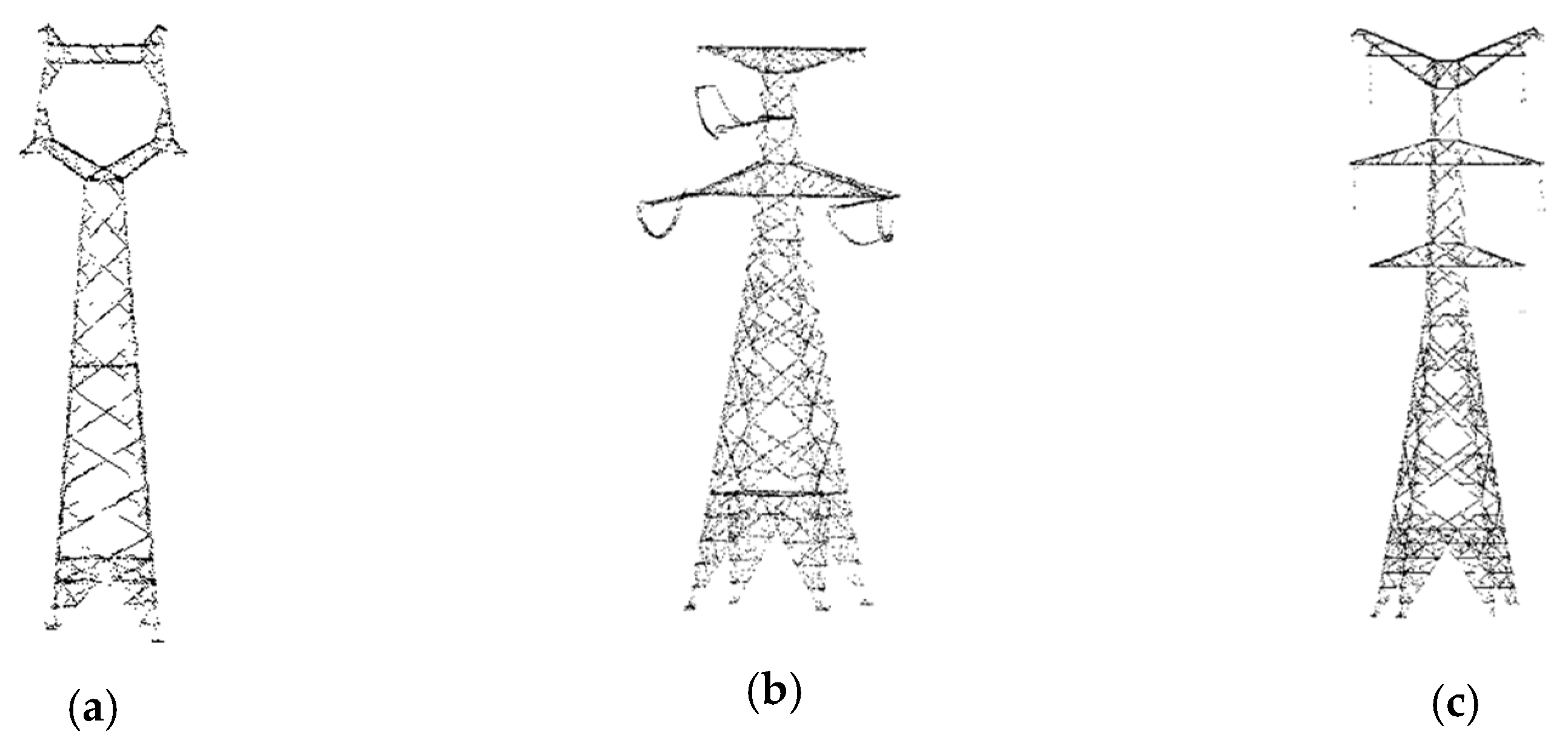
Figure 3.
The pylon types of datasets: (a) Pylon belongs to the line in Figure 1a; (b) pylon belongs to the line in Figure 1c; (c) pylon belongs to the line in Figure 1d. Three different types of pylon are included.

Figure 4.
The complete flowchart of our study. This flowchart has been divided into two parts. The left box is the basic classification framework and the right box lists the main experiments, including comparison among classifiers, balanced versus unbalanced learning, comparison between feature sets, and sensitivity analysis of neighborhood radius. All classifiers, feature sets and class distribution tested are listed in the dotted box.

Figure 5.
Neighborhood types used in feature extraction: (a) Cylinder neighborhood C, (b) spherical neighborhood S (hollow point: Center point, r: Neighborhood radius).
Figure 5.
Neighborhood types used in feature extraction: (a) Cylinder neighborhood C, (b) spherical neighborhood S (hollow point: Center point, r: Neighborhood radius).

Figure 6.
The classification results of site I with different classifiers: (a) the point clouds colored by the true labels; (b) the point clouds colored by the KNN prediction results; (c) the point clouds colored by the LR prediction results; (d) the point clouds colored by the RF prediction results; (e) the point clouds colored by the GBDT prediction results. The black box is an area of obvious misclassification.


Figure 7.
The classification results of site II with different classifiers. (a) The point clouds colored by the true labels; (b) the point clouds colored by the KNN prediction results; (c) the point clouds colored by the LR prediction results; (d) the point clouds colored by the RF prediction results; (e) the point clouds colored by the GBDT prediction results. The black box is an area of obvious misclassification.


Figure 8.
The classification results of site III with different classifiers: (a) The point clouds colored by the true labels; (b) the point clouds colored by the KNN prediction results; (c) the point clouds colored by the LR prediction results; (d) the point clouds colored by the RF prediction results; (e) the point clouds colored by the GBDT prediction results. The black box is an area of obvious misclassification.

Figure 9.
The pylons are colored by the true labels: (a) Pylon type in the training set; (b) pylon type-I in site II; (c) pylon type-III in site III.
Figure 9.
The pylons are colored by the true labels: (a) Pylon type in the training set; (b) pylon type-I in site II; (c) pylon type-III in site III.

Figure 10.
The classification results of pylon type-I with different classifiers (feature set = , class distribution = unbalanced, R = 1.5 m): (a) The pylon is colored by the KNN prediction results; (b) the pylon is colored by the LR prediction results; (c) the pylon is colored by the RF prediction results; (d) the pylon is colored by the GBDT prediction results.

Figure 11.
The classification results of pylon type-II with different classifiers( feature set = , class distribution = unbalanced, R = 1.5 m): (a) The pylon is colored by the KNN prediction results; (b) the pylon is colored by the LR prediction results; (c) the pylon is colored by the RF prediction results; (d) the pylon is colored by the GBDT prediction results.

Figure 12.
Oversampling results of the building, pylon and power line class: (a) Oversampled building, (b) oversampled pylon, (c) oversampled power line. The original points are colored with blue, while the synthetic points are colored with red.
Figure 12.
Oversampling results of the building, pylon and power line class: (a) Oversampled building, (b) oversampled pylon, (c) oversampled power line. The original points are colored with blue, while the synthetic points are colored with red.

Figure 13.
The sensitivity analysis of neighborhood radius for different classes based on the RF classifier.
Figure 13.
The sensitivity analysis of neighborhood radius for different classes based on the RF classifier.


Table 1.
Details about data acquisition.
| Sensor | Flight Height | Swath | Flight Speed | Field of View | Scanning Speed | Laser Pulse Rate | Laser Beam Divergence | Number of Returns |
|---|---|---|---|---|---|---|---|---|
| RIEGL VUX-1 | 200 m | 400 m | 30 km/h | 330° | 200 lines/s | 550 kHz | 0.5 mrad | 4 |
Table 2.
Overview of the Datasets.
| Dataset | Area/m2 | Density (pt/m2) | Points | ||||||
|---|---|---|---|---|---|---|---|---|---|
| Ground | Vegetation | Pylon | Power Line | Building | SUM | ||||
| Training Set | 907 × 90 | 52 | 3,763,849 | 2,345,327 | 321,306 | 26,877 | 49,912 | 6,199,950 | |
| 60.71% | 37.83% | 5.18% | 0.43% | 0.81% | 100% | ||||
| Test Set | I | 535 × 90 | 44 | 1,782,922 | 1,004,471 | 5850 | 15,391 | 10,381 | 2,819,021 |
| 63.25% | 35.63% | 0.21% | 0.55% | 0.37% | 100% | ||||
| II | 397 × 90 | 73 | 1,586,186 | 1,848,031 | 20,509 | 20,688 | 222,033 | 3,697,447 | |
| 42.90% | 50.00% | 0.60% | 0.60% | 6.00% | 100% | ||||
| III | 937 × 80 | 41 | 2,464,418 | 1,246,571 | 62,074 | 162,771 | 43,777 | 3,979,611 | |
| 61.93% | 31.32% | 1.56% | 4.09% | 1.10% | 100% | ||||
Table 3.
Feature vector description. The first column represents the basis of feature computing, the second column is the feature name, the third column is the feature abbreviation, the fifth column is the feature computing method, and the last column is the description of the feature meaning.
Table 3.
Feature vector description. The first column represents the basis of feature computing, the second column is the feature name, the third column is the feature abbreviation, the fifth column is the feature computing method, and the last column is the description of the feature meaning.
| Category | Feature | Abbreviation | Equation | Description |
|---|---|---|---|---|
| Eigenvalue | Sum | SU | The sum of the eigenvalues | |
| Omnivariance | OM | - | ||
| Eigenentropy | EI | The entropy of eigen | ||
| Anisotropy | AN | The homogeneity distribution of points in three directions | ||
| Planarity | PL | A measure of planar-likeness | ||
| Linearity | LI | A measure of linear-likeness | ||
| Surface Variation | SUV | A measure of surface roughness | ||
| Sphericity | SP | A measure of spherical-likeness | ||
| Verticality | VE | A measure of vertical-likeness | ||
| Density | Point Density | PD | The density of points within S | |
| Density Ratio | DR | The ratio of the point density in S and in its projection plane | ||
| Height | Vertical Range | VR | Height difference in C | |
| Height Above | HA | The height difference between the current point and the lowest point in C | ||
| Height Below | HB | The height difference between the current point and the highest point in C | ||
| Sphere Variance | SPV | Standard deviation of height difference in S | ||
| Cylinder Variance | CV | Standard deviation of height difference in C | ||
| Vertical Profile | ContiOffSegment | CFS | - | Maximum number of discrete segments |
| ContiOnSegment | COS | - | Maximum number of consecutive segments | |
| MaxHeightDev | MHD | Maximum height difference of the barycenter | ||
| MaxPtsNumDev | MPD | Maximum height difference of the mean height | ||
| OnSegmentNum | OS | - | Number of segments containing points |
Table 4.
Classification performance for the different classifiers (feature set = , class distribution = unbalanced, R = 1.5 m). Three performance measures are shown in this table. P denotes the macro precision, R denotes the macro recall, and F denotes the macro F1. Bold denotes best results for each performance metric in each test set.
| Dataset | Classifiers | Performance Measures | ||
|---|---|---|---|---|
| Macro Precision (P, %) | Macro Recall (R, %) | Macro F1 (F, %) | ||
| Site I | KNN | 77.76 | 81.36 | 78.24 |
| LR | 80.05 | 69.93 | 73.71 | |
| RF | 82.16 | 83.15 | 82.33 | |
| GBDT | 79.99 | 82.80 | 80.45 | |
| Site II | KNN | 86.59 | 78.55 | 81.00 |
| LR | 89.87 | 65.58 | 69.78 | |
| RF | 92.70 | 84.60 | 87.72 | |
| GBDT | 91.88 | 83.12 | 86.34 | |
| Site III | KNN | 81.34 | 70.11 | 73.50 |
| LR | 78.29 | 62.52 | 68.47 | |
| RF | 74.71 | 67.00 | 66.01 | |
| GBDT | 78.52 | 76.35 | 76.59 | |
| Average | KNN | 81.90 | 76.67 | 77.58 |
| LR | 82.74 | 66.01 | 70.65 | |
| RF | 83.19 | 78.25 | 78.69 | |
| GBDT | 83.46 | 80.76 | 81.13 | |
Table 5.
The confusion matrix and performance measures of site I (classifier = RF, feature set = , class distribution = unbalanced, R = 1.5 m).
Table 5.
The confusion matrix and performance measures of site I (classifier = RF, feature set = , class distribution = unbalanced, R = 1.5 m).
| Class | Ground | Vegetation | Pylon | Power Line | Building | PRECISION RATE (PRE, %) |
|---|---|---|---|---|---|---|
| Ground | 1,685,297 | 165,815 | 151 | 0 | 3098 | 90.88 |
| Vegetation | 97,524 | 834,939 | 2,005 | 69 | 6,215 | 88.75 |
| Pylon | 0 | 1 | 3,655 | 30 | 0 | 99.16 |
| Power line | 0 | 57 | 22 | 15,287 | 0 | 99.49 |
| Building | 101 | 3,659 | 17 | 11 | 1068 | 21.99 |
| Recall rate (REC, %) | 94.52 | 83.12 | 62.48 | 99.29 | 10.29 |
Table 6.
The confusion matrix and performance measures of site II (classifier = RF, feature set = , class distribution = unbalanced, R = 1.5 m).
Table 6.
The confusion matrix and performance measures of site II (classifier = RF, feature set = , class distribution = unbalanced, R = 1.5 m).
| Class | Ground | Vegetation | Pylon | Power Line | Building | PRE (%) |
|---|---|---|---|---|---|---|
| Ground | 1,537,494 | 366,825 | 43 | 1 | 35,103 | 79.27 |
| Vegetation | 45,978 | 1,474,955 | 3844 | 1 | 31,213 | 94.79 |
| Pylon | 0 | 3 | 15,813 | 196 | 0 | 98.76 |
| Power line | 0 | 16 | 809 | 20,490 | 0 | 96.13 |
| Building | 2,714 | 6232 | 0 | 0 | 155,717 | 94.57 |
| REC(%) | 96.93 | 79.81 | 77.1 | 99.04 | 70.13 |
Table 7.
The confusion matrix and performance measures of site III (classifier = RF, feature set = , class distribution = unbalanced, R = 1.5 m).
Table 7.
The confusion matrix and performance measures of site III (classifier = RF, feature set = , class distribution = unbalanced, R = 1.5 m).
| Class | Ground | Vegetation | Pylon | Power Line | Building | PRE (%) |
|---|---|---|---|---|---|---|
| Ground | 2,427,197 | 327,024 | 499 | 0 | 18,829 | 87.51 |
| Vegetation | 36,798 | 915,267 | 16,302 | 53,945 | 17,513 | 88.02 |
| Pylon | 411 | 1,192 | 41,800 | 3,601 | 0 | 88.93 |
| Power line | 0 | 97 | 1,187 | 91,748 | 0 | 98.62 |
| Building | 12 | 2,991 | 2,286 | 13,477 | 7,435 | 28.38 |
| REC(%) | 98.49 | 73.42 | 67.34 | 56.37 | 16.98 |
Table 8.
Classification performance for different sampling references (feature set = F0, classifier = RF, R = 1.5 m).
Table 8.
Classification performance for different sampling references (feature set = F0, classifier = RF, R = 1.5 m).
| Sampling Reference Value | Performance Measures | |
|---|---|---|
| Mean Score (%) | Time/s | |
| Original training set | 91.28 | 3284 |
| 50,000 | 93.46 | 77 |
| 100,000 | 97.24 | 179 |
| 150,000 | 97.32 | 291 |
Table 9.
The resampled training dataset. Table shows the number of points and proportion per class after resampling.
Table 9.
The resampled training dataset. Table shows the number of points and proportion per class after resampling.
| Class | Resampled Dataset | |
|---|---|---|
| Ground | 100,000 | 19.26% |
| Vegetation | 100,000 | 19.26% |
| Pylon | 111,880 | 21.55% |
| Power line | 107,508 | 20.71% |
| Building | 99,824 | 19.23% |
| SUM | 519,212 | 100% |
Table 10.
Classification performance for different class distributions (classifier = RF, feature set = , R = 1.5 m). Three performance measures are shown in the table. The symbol Δ denotes the difference between the measures obtained by balanced and unbalanced learning. P denotes macro precision, R denotes macro recall, and F denotes the macro F1.
| Dataset | Class Distribution | Performance Measures | ||
|---|---|---|---|---|
| P (%) | R (%) | F (%) | ||
| Site I | Unbalanced | 82.16 | 83.15 | 82.16 |
| Balanced | 75.81 | 87.34 | 76.95 | |
| Δ | −6.35 | +4.19 | −5.21 | |
| Site II | Unbalanced | 89.87 | 65.58 | 89.87 |
| Balanced | 84.59 | 87.38 | 85.58 | |
| Δ | −5.28 | +21.80 | −4.29 | |
| Site III | Unbalanced | 74.71 | 67.00 | 74.71 |
| Balanced | 67.81 | 72.68 | 64.10 | |
| Δ | −6.9 | +5.68 | −10.61 | |
Table 11.
Variation of F1 values for different classes and class distributions (classifier = RF, feature set = , R = 1.5 m). Δ denotes the difference between the measures obtained by balanced and unbalanced learning.
Table 11.
Variation of F1 values for different classes and class distributions (classifier = RF, feature set = , R = 1.5 m). Δ denotes the difference between the measures obtained by balanced and unbalanced learning.
| Dataset | Class Distribution | F1 (%) | ||||
|---|---|---|---|---|---|---|
| Ground | Vegetation | Pylon | Power Line | Building | ||
| Site I | Unbalanced | 93.54 | 87.74 | 97.89 | 99.93 | 32.54 |
| Balanced | 92.38 | 86.71 | 94.14 | 99.91 | 11.6 | |
| Δ | −1.16 | −1.03 | −3.75 | −0.02 | −20.94 | |
| Site II | Unbalanced | 87.22 | 86.66 | 86.6 | 97.56 | 80.54 |
| Balanced | 87.81 | 87.04 | 81.13 | 95.82 | 76.09 | |
| Δ | +0.59 | +0.38 | −5.47 | −1.74 | −4.45 | |
| Site III | Unbalanced | 93.15 | 82.9 | 49.62 | 51.03 | 53.38 |
| Balanced | 92.67 | 83.22 | 47.99 | 60.53 | 36.07 | |
| Δ | −0.48 | +0.32 | −1.63 | +9.50 | −17.31 | |
Table 12.
The classification performance for different feature sets (classifier = RF, class distribution = unbalanced, R = 1.5 m). Three performance measures are shown in the table. P denotes the macro precision, R denotes the macro recall, and F denotes the macro F1. Bold denotes best results for each performance metric in each test set.
| Dataset | Feature Set | Performance Measures | ||
|---|---|---|---|---|
| P (%) | R (%) | F (%) | ||
| Site I | 82.16 | 83.15 | 82.33 | |
| 77.67 | 79.01 | 77.62 | ||
| 81.62 | 82.37 | 81.66 | ||
| Site II | 89.87 | 65.58 | 89.87 | |
| 88.24 | 77.71 | 81.51 | ||
| 92.14 | 82.86 | 86.36 | ||
| Site III | 74.71 | 67.00 | 74.71 | |
| FPCA | 70.69 | 62.92 | 65.04 | |
| 74.48 | 63.32 | 63.36 | ||
Table 13.
The sensitivity analysis of neighborhood radius for feature extraction about each class (classifier = RF, class distribution = unbalanced, test set = site III). Bold denotes best results for each class.
Table 13.
The sensitivity analysis of neighborhood radius for feature extraction about each class (classifier = RF, class distribution = unbalanced, test set = site III). Bold denotes best results for each class.
| Radius/m | 1.5 | 2.5 | 3.5 | 4.5 | 5.5 | |
|---|---|---|---|---|---|---|
| F1(%) | ||||||
| Ground | 86.85 | 85.37 | 85.08 | 84.14 | 84.45 | |
| Vegetation | 86.22 | 83.86 | 83.40 | 82.30 | 82.86 | |
| Pylon | 80.18 | 81.14 | 85.48 | 89.95 | 67.65 | |
| Power line | 96.74 | 97.70 | 96.65 | 96.57 | 95.65 | |
| Building | 81.69 | 84.21 | 85.29 | 84.84 | 83.89 | |
| Mean | 86.34 | 86.46 | 87.18 | 87.56 | 82.90 | |
© 2019 by the authors. Licensee MDPI, Basel, Switzerland. This article is an open access article distributed under the terms and conditions of the Creative Commons Attribution (CC BY) license (http://creativecommons.org/licenses/by/4.0/).
Share and Cite
MDPI and ACS Style
Peng, S.; Xi, X.; Wang, C.; Dong, P.; Wang, P.; Nie, S. Systematic Comparison of Power Corridor Classification Methods from ALS Point Clouds. Remote Sens. 2019, 11, 1961. https://doi.org/10.3390/rs11171961
AMA Style
Peng S, Xi X, Wang C, Dong P, Wang P, Nie S. Systematic Comparison of Power Corridor Classification Methods from ALS Point Clouds. Remote Sensing. 2019; 11(17):1961. https://doi.org/10.3390/rs11171961
Chicago/Turabian StylePeng, Shuwen, Xiaohuan Xi, Cheng Wang, Pinliang Dong, Pu Wang, and Sheng Nie. 2019. "Systematic Comparison of Power Corridor Classification Methods from ALS Point Clouds" Remote Sensing 11, no. 17: 1961. https://doi.org/10.3390/rs11171961
Note that from the first issue of 2016, this journal uses article numbers instead of page numbers. See further details here.