A Hybrid Model Integrating Spatial Pattern, Spatial Correlation, and Edge Information for Image Classification

Abstract

This paper develops a novel hybrid model that integrates three spatial contexts into probabilistic classifiers for remote sensing classification. First, spatial pattern is introduced using multiple-point geostatistics (MPGs) to characterize the general distribution and arrangement of land covers. Second, spatial correlation is incorporated using spatial covariance to quantify the dependence between pixels. Third, an edge-preserving filter based on the Sobel mask is introduced to avoid the over-smoothing problem. These three types of contexts are combined with the spectral information from the original image within a higher-order Markov random field (MRF) framework for classification. The developed model is capable of classifying complex and diverse land cover types by allowing effective anisotropic filtering of the image while retaining details near edges. Experiments with three remote sensing images from different sources based on three probabilistic classifiers obtained results that significantly improved classification accuracies when compared with other popular contextual classifiers and most state-of-the-art methods.

1. Introduction

Land cover classification is one of the most common remote sensing applications. Traditional classification methods based on spectral information of individual pixels may result in undesirable artifacts (e.g., salt-and-pepper effects) as reported in many studies [1,2]. According to Tobler’s first law of geography, everything is related to everything else, but near things are more related than distant things [3]. Therefore, many contextual classification methods have been proposed to improve classification results by taking into account information from neighboring pixels (i.e., spatial contexts) [4,5,6,7,8,9,10,11,12,13]. Contextual classification methods are roughly grouped into four categories: Filtering-based, object-based, spatial weight based, and probabilistic graphical model (PGM)-based methods [14,15].

Filtering-based methods apply a sliding window (i.e., filter) to an image with the central pixel of the window becoming a function of the features of all the pixels within the filter. The most popular filter-based method is majority voting, which smooths noise by assigning the most common class in the filter to the central pixel. Other filtering-based methods include the Gaussian filter, bilateral filter [16], anisotropic diffusion [17], etc. However, filtering-based methods may smear the boundary of geographic objects, especially with a large sliding window size. This deficiency can be addressed with well-known object-based image analysis (OBIA). In this approach, image segmentation is applied first to form homogeneous patches or image segments. Then, a segment is assigned to an object class using voting strategies based on the spatial contexts of all the pixels within the segment [18,19,20,21]. This differs from traditional object-based classification, which assumes segments are uniform inside. The object-based methods can result in clear boundaries, but the classification results are greatly influenced by the quality of the segmentation, which has been a problem [22]. Spatial weight-based methods characterize spatial contexts using models (e.g., geostatistical models) that assign greater spatial weight in classification to nearby pixels than more distant ones [3,23,24,25]. Multiple-point geostatistics (MPGs) is an enhancement to traditional geostatistical models. It extracts spatial patterns by characterizing the joint relationship of multiple points [26] and has been employed for both improving classifiers [27,28] and post-processing of classification results [29]. Spatial weight-based methods are less common because the determination of the most suitable model is subjective and usually requires the involvement of expert knowledge.

PGM is a probabilistic model that can express the conditional dependency between random variables. Markov random fields (MRFs) is the most common PGM-based method. MRF models consider contexts by awarding neighboring pixels with the same label and penalizing those with different labels. It can iteratively optimize classification results and has often proven able to deliver superior classification accuracy [30,31]. Combining MRFs with other models to improve classification has been widely studied. For example, Sun et al. [32] and Khodadadzadeh et al. [33] introduced MRFs for hyperspectral image classification by combining multinomial logistic regression with total variation regularization and mixed pixel modeling. Some recent work has explored the data fusion capability of MRF by combining multiple spectral with spatial features [34] and edge information [35]. Another promising trend is to expand the neighborhood of the MRF model hierarchically and spatially. Multi-resolution techniques, such as quad-tree or wavelet transform, are employed in the hierarchical MRF model [36,37]. Object-based MRF [38] and higher-order MRF [39,40] can model long-range spatial interactions between variables, providing more knowledge about the contexts of a scene.

In general, the above contextual classifications have the following limitations. First, most contexts (e.g., neighborhood information) do not incorporate spatial correlation and joint spatial relationships. Second, most contextual classification models focus on one specific context. A model is needed that can integrate several different and sometimes complementary spatial contexts into the classification. Third, it is difficult to control the balance between noise smoothing and detail retention in most contextual classification methods. Finally, there is still much room for improving the MRF-based methods despite their aforementioned success. For example, a higher-order MRF is rarely used in land cover classification, and the strength of interactions in different orders has not been extensively explored.

To address the above problems, a novel model that aims to integrate various spatial contexts was developed. It combines spatial pattern, spatial correlation, and edge information within an MRF framework to improve the traditional probabilistic classifications. Spatial pattern reflects the general distribution and arrangement of land cover classes, whereas spatial correlation quantifies pairwise spatial dependence of the pixels. Spatial pattern and spatial correlation are complementary, and when combined may potentially provide an anisotropic filtering based on the contexts of land cover distributions and pixel dependency. In addition, the over-smoothing problem is addressed by introducing an edge-preserving filter to retain detail near boundaries. A higher-order multi-grid MRF model is used for integration in order to capture long-range contexts and reduce computation load. The model can be utilized in traditional probabilistic classifiers, such as maximum likelihood classification (MLC), support vector machine (SVM), and k-nearest neighbor (KNN), to improve the accuracy of original classifiers that use spectral information only.

2. Material and Methods

2.1. Datasets and Study Areas

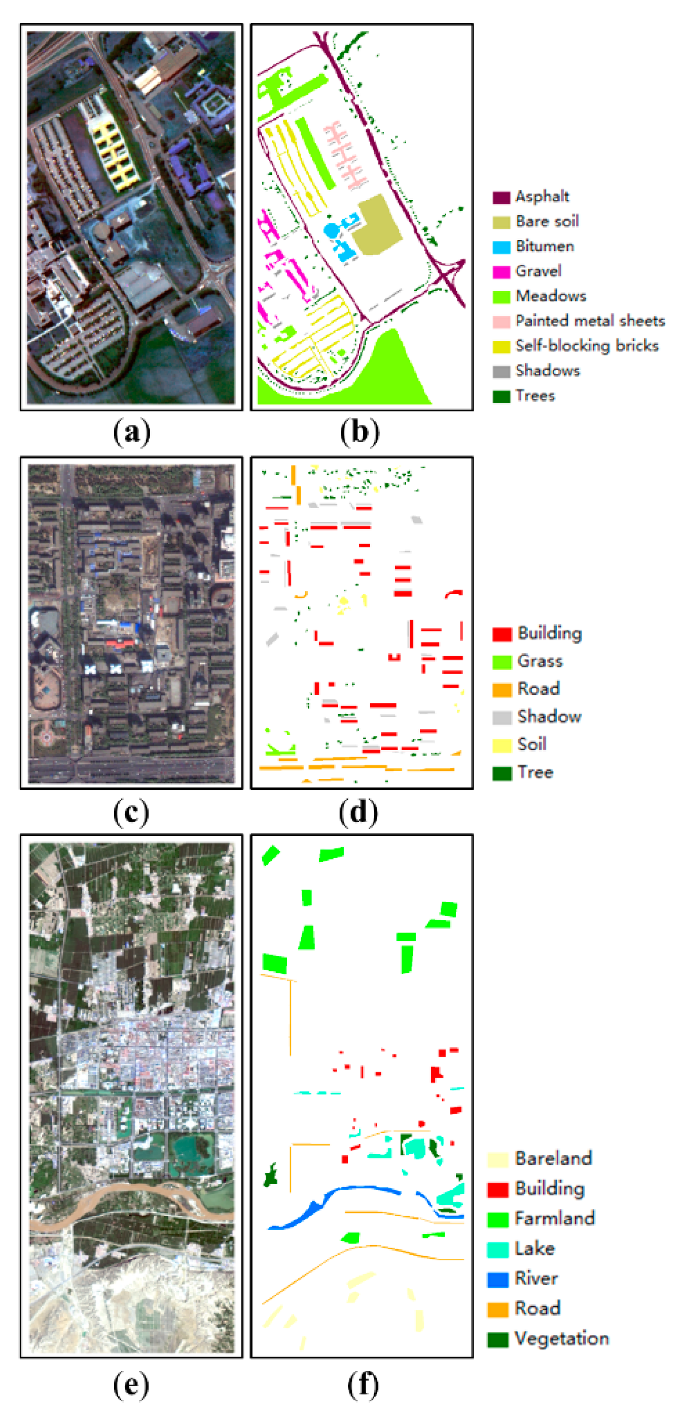
The developed model was tested on three differing remote sensing images, including hyperspectral, and multispectral images with medium and high spatial resolutions. The three images shown in Figure 1 (each corresponding to a study area) were used as the experimental datasets. The study areas feature different environments with differing spatial distributions of their land covers and the images were derived from different sensors, thus providing a robust test of the new approach.

The first image covers the University of Pavia in Italy, acquired by the hyperspectral ROSIS sensor (The scene is available online at http://www.ehu.eus/ccwintco/index.php?title=Hyperspectral_Remote_Sensing_Scenes). The image has 103 bands (after removing 12 noisy channels) with a spectral coverage ranging from 0.43 to 0.86 μm. There are 610 × 340 pixels and the spatial resolution is 1.3 m per pixel. A principal component analysis was employed to reduce the dimensionality of the spectral bands to six principal components for classification purposes, the accumulated contribution of which reached 99.5%. The second image is a high spatial resolution image acquired by the IKONOS satellite (4-band bundle, standard 2A) over the Beijing urban area (39°57′55″–39°58′28″N, 116°24ʹ5′–116°24′49″E) in May 2000. The image has 850 × 551 pixels, and the spatial resolution of the four multispectral bands was increased to 1 m using the Gram–Schmidt pansharpening method applied to the panchromatic band. The third image is a Landsat 8 OLI image subset (level 1T) of medium spatial resolution acquired over Zhongwei City (37°26′38″–37°33′43″E, 105°8′47″–105°17′41″E), Ningxia Hui Autonomous Region, China on 22 April 2017. The image has 875 × 350 pixels, with the spatial resolution of the multispectral bands enhanced to 15 m again using the Gram–Schmidt pansharpening method.

The training data for classification were selected from the ground-truth data using stratified random sampling. The sampling scheme incorporates class imbalance in order to reduce the effects of small sample size on some classifiers (e.g., KNN). For all three images, the training samples accounted for a very small proportion (<1%) of the ground-truth data, and the rest were used for testing. Sample information is provided in

Table 1. The training and testing samples per class for the three study areas.

ROSIS			IKONOS			Landsat
Class	Training	Testing	Class	Training	Testing	Class	Training	Testing
Asphalt	45	6586	Building	57	15,956	Bare land	24	2298
Bare soil	16	5013	Grass	17	1315	Building	35	1626
Bitumen	18	1312	Road	33	6962	Farmland	38	6742
Gravel	24	2075	Shadow	38	6184	Lake	20	2764
Meadows	39	18,610	Soil	30	1612	River	11	2103
Painted metal sheets	14	1331	Tree	61	3445	Road	27	1750
Self-blocking bricks	68	3614				Vegetation	17	1329
Shadows	44	903
Trees	80	2984
Total	348	42,428	Total	236	35,474	Total	172	18,612

.

2.2. Methods

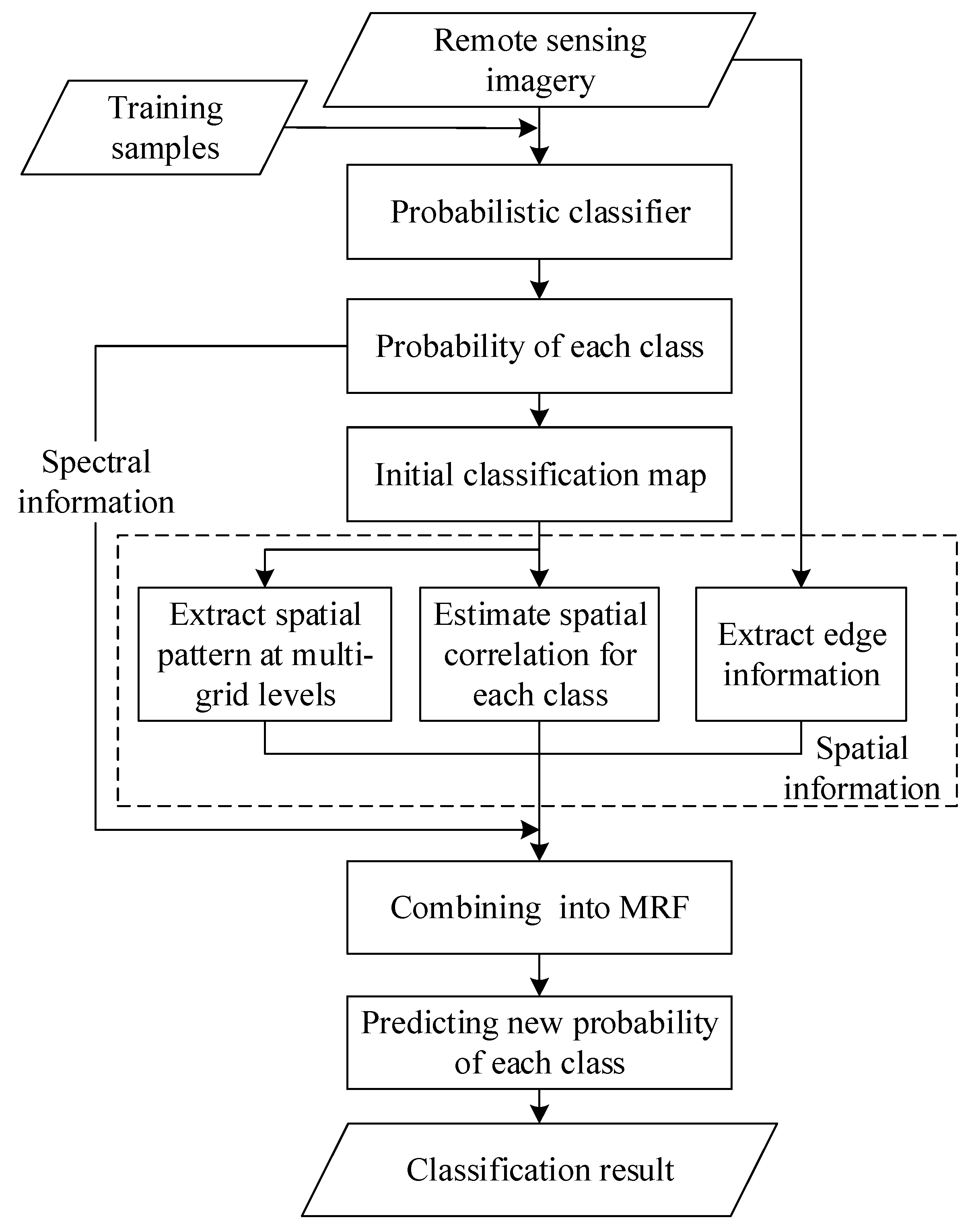
Using an MRF framework, the developed model integrates the spatial pattern (i.e., spatial distribution, spatial arrangement) of land cover classes, the spatial correlation within each land cover class, and the edge information of geographic objects with the original spectral information of the image. The spatial pattern and spatial correlation are derived from prior knowledge, whereas the edge information is directly extracted from the remote sensing images. These contexts are then combined with the spectral information in an MRF framework before being further classified. The flowchart of the new classification method is shown in Figure 2. For simplicity, the abbreviation MIX-E is used to refer to this mixed-contexts model.

The prior knowledge required for the spatial pattern and spatial correlation components is provided by an initial classification map produced using traditional probabilistic classification of a remote sensing image with labeled training samples. The result is then taken as a training image (TI), a term used in MPG representing prior knowledge about the underlying scene [26]. The spatial pattern of classes in the form of multiple-point (MP) probabilities are then extracted by data templates at multi-grid levels. Simultaneously, spatial correlation is measured by spatial covariance for each class using distance lags compiled from the same data templates. A Sobel mask is applied as an edge-preserving filter to compute gradients for spectral bands and to constrain smoothing effects near boundaries. To derive the final classification result, all the extracted contexts are integrated with the spectral information in a higher-order MRF model for optimization. The details are explained in the following subsections.

2.2.1. Multi-Grid Template

A data template, T_N, is a moving window composed of N pixels, u_n (n = 1, …, N). When a TI is given, the data template, T_N, is used to scan the TI to capture spatial pattern, termed a data event in MPG [41]. In this study, a square (e.g., 9 × 9) T_N is used. The data template can also be expressed as T_N = {h₁, …, h_N}, where h_n (n = 1, …, N) is a directional distance vector between u_n and the central node in the data template. In the following text, u stands for a pixel in general, and u_i stands for a central pixel in the data template, T_N. The neighboring pixels, u_n, around u_i in T_N are referred to as Nei{u_i}, where u_n $\in$ Nei{u_i}.

Long-range structures can be captured by using a large template, but that may cause the details of the structures to be lost and also exerts an undue burden on computer resources [42]. Therefore, a multi-grid strategy is employed [43] to achieve the operational range of a large data template. The number, L, represents a new multi-grid sparse template, $T_N^L$, at level L, such that $T_N^L=\left\{2^{L-1}{h}_1,\dots ,2^{L-1}{h}_N\right\}$. The template, $T_N^L$, has the same number of vectors and geometric configuration as T_N, but with a larger spatial extent (i.e., the template size is of (2^L + 1) × (2^L + 1) pixels), and hence can capture long-range structures without increasing the number of pixels. An example of a data template of 3 × 3 pixels with a multi-grid level, L, of 5 is shown in Figure 3. This template has 33 × 33 pixels, but only those pixels at multi-grid levels (i.e., lag distance h = 1, 2, 4, 8, and 16) are used to extract patterns.

2.2.2. Extraction of Spatial Pattern

The number of occurrences of a pattern can be calculated when the TI is scanned by the data template. The relative frequency of the pattern can then be converted to a multiple-point (MP) probability. The data template scans the image L times to derive the MP probability at L multi-grid levels. The MP probability of a pixel, u, belonging to class c at a single grid level is defined as:

$$P_{\mathrm{MP}}\left(u=c\right)=\frac{1}{M\left(c\right)}{\displaystyle \sum _{i=1}^{M}I\left(\mathrm{Nei}\left\{u_i\right\}=c\right)},$$

(1)

where M is the number of pixels in the image, and M(c) is the number of pixels belonging to class c. The indicator function, I(.), takes a value of one if the condition is satisfied, otherwise zero. In Equation (1), the indicator contributes to the numerator only when all the neighboring pixels, Nei{u_i}, at the current grid level belong to the same class c. Therefore, the MP probability of each land cover class reflects whether the class’s distribution is clustered or dispersed. A higher MP probability value for a class indicates a greater likelihood of a clustered distribution, whereas a lower value suggests it is more likely distributed as individual pixels (noise).

2.2.3. Estimation of Spatial Correlation

Spatial correlation is measured by the spatial covariance, also referred to as class-conditional probability. The class-conditional probability of a pixel, u, belonging to class c given a neighboring pixel is estimated as:

$$P_{\mathrm{cov}}\left(u=c\right)=\frac{{\displaystyle \sum _{i=1}^{M}I\left(u_n=c|u_i=c\right)}}{{\displaystyle \sum _{i=1}^{M}I\left(u_i=c\right)}}.$$

(2)

Spatial covariance is based on the pairwise correlation in a data template, which means the indicator contributes to the numerator when the conditional neighboring pixel, u_n, has the same class c, with the central pixel, u_i. Previous work has commonly used geostatistical models to fit class-conditional probability plots derived from sample data [23]. Here, the class-conditional probabilities themselves provide spatial covariance measures since they are estimated from the TI via the data template rather than from sample data. Coupled with the multi-grid levels, the neighboring pixel, u_n, implies the direction and distance from u_i in the data template. Therefore, each land cover class has different spatial covariance values at different lag distances (i.e., L intervals) and in different directions. The spatial covariance of a land cover class is usually larger for two pixels separated by a smaller distance than a larger distance, whereas the noise pattern is presumed to have a constant spatial covariance.

2.2.4. Extraction of Edge Information

Edge information in the form of gradients, ρ, is extracted directly from the remote sensing images, where ρ is the convolution result of the original image, U, and the Sobel mask, G. The masks are applied in horizontal, vertical, and two diagonal directions using a 3 × 3 filter [44]. The gradient in each direction is computed as the sum of the gradients of each spectral band, and the resulting gradient, ρ, at location u_i is computed as the average of all the directional gradients. To integrate the edge information into the classification, a fuzzy no-edge/edge function is defined as [35,45]:

$$\epsilon \left(u_i\right)=1-\frac{\rho \left(u_i\right)}{\alpha +\rho \left(u_i\right)},$$

(3)

where ε(.) is the fuzzy no-edge/edge function at location u_i and α is a positive parameter controlling the edge–strength threshold.

2.2.5. The MIX-E Model

For a probabilistic classification based on MRF, the decision rule is the maximum a posteriori (MAP) estimation. According to the Bayesian rule and the log-linear property, solving the MAP $P\left(c|x\right)$ (i.e., the probability of the pixel belonging to class c given the feature vector, x) is equivalent to minimizing the energy functions, E_spectral and E_spatial [15,46]:

$$c=\arg \max P\left(c|x\right)=\arg \min \left(E_{\mathrm{spectral}}+E_{\mathrm{spatial}}\right),$$

(4)

with:

$$\begin{array}{c}{E}_{\mathrm{spectral}}=-\ln P_{\mathrm{spectral}}\left(\mathbf{x}|c\right)\\ E_{\mathrm{spatial}}=-\ln P_{\mathrm{spatial}}\left(c\right)\end{array}.$$

(5)

The spectral term, $P_{\mathrm{spectral}}\left(x|c\right)$, is a probability density function (PDF) derived from different classifiers. For example, MLC assumes that the PDF follows a Gaussian distribution. For other non-Bayesian classifiers, such as SVM and KNN, estimating the PDF is not as straightforward. Previous efforts to combine non-Bayesian classifiers and MRF have used other probability forms as alternatives to PDFs [47,48]. For the MIX-E model developed here, the pairwise coupling of probability is taken as the spectral information for the SVM classifier [49]; probabilities are estimated using an inverse distance weighted scheme [50] for the KNN classifier.

The spatial term, $P_{\mathrm{spatial}}\left(c\right)$, of u_i is decided by the classes in its neighborhood, Nei{u_i}. In the MRF method, the spatial term is established by:

$$P_{\text{spatial-MRF}}\left(c\right)=\frac{1}{Z}\exp \left(-V_c\right)=\frac{1}{Z}\exp \left\{{\displaystyle \sum _{u_n\in \mathrm{Nei}\left\{u_i\right\}}\beta \cdot \left[1-I\left(u_i=u_n\right)\right]}\right\},$$

(6)

where V_c is called the potential function of the clique. β is a smoothing parameter representing the degree to which the occurrence of a class for a pixel is affected by its neighboring pixels, usually based on 4-connectivity (first order) or 8-connectivity (second order). Z is a normalization constant. The indicator function, $I\left(u_i=u_n\right)$, takes a value of one or zero based on whether the class of pixel u_i and its neighboring pixel, u_n ∈ Nei{u_i}, is the same or not.

In the MIX-E model, the MRF works on a higher-order multi-grid data template, incorporating the spatial pattern in the form of MP probabilities, spatial correlation in the form of spatial covariance, and edge information. According to Equations (1) to (3), the spatial term is thus defined as:

$$\begin{array}{l}\hspace{1em}{P}_{\text{spatial-MIX-E}}\left(c\right)\\ =P_{\text{spatial-MIX-E}}\left(u_i=c|\mathrm{Nei}\left\{u_i\right\}\right)\\ =\frac{1}{Z}\exp \left\{\frac{1}{L}{\displaystyle \sum _{l=1}^L{\displaystyle \sum _{u_{n(l)}\in {\mathrm{Nei}}_{(l)}\left\{u_i\right\}}\beta \cdot \epsilon \left(u_i\right)\cdot \left[w{P}_{\mathrm{MP}(l)}\left(u_i=c\right)+\left(1-w\right)P_{\mathrm{cov}(l)}\left(u_i=c\right)\right]\cdot \left[1-I\left(u_i=u_{n(l)}\right)\right]}}\right\}\\ =\frac{1}{Z}\exp \{\frac{1}{L}{\displaystyle \sum _{l=1}^L{\displaystyle \sum _{u_{n(l)}\in {\mathrm{Nei}}_{(l)}\left\{u_i\right\}}\beta \cdot \left[1-\frac{\rho \left(u_i\right)}{\alpha +\rho \left(u_i\right)}\right]}\cdot [\frac{w}{M\left(c\right)}{\displaystyle \sum _{i=1}^{M}I\left({\mathrm{Nei}}_{(l)}\left\{u_i\right\}=c\right)}}\\ +\left(1-w\right)\frac{{\displaystyle \sum _{i=1}^{M}I\left(u_{n(l)}=c|u_i=c\right)}}{{\displaystyle \sum _{i=1}^{M}I\left(u_i=c\right)}}]\cdot \left[1-I\left(u_i=u_{n(l)}\right)\right]\}\end{array},$$

(7)

where w is a proportional weight ranging from 0 to 1. l stands for the lth grid level, and L is the number of total multi-grid levels.

Combining Equations (4), (5), and (7), class c at location u_i is predicted as:

$$\begin{array}{l}c=\arg \min \{-\ln P_{\mathrm{spectral}}\left(x|c\right)-\frac{1}{L}{\displaystyle \sum _{l=1}^L{\displaystyle \sum _{u_{n(l)}\in {\mathrm{Nei}}_{(l)}\left\{u_i\right\}}\beta \cdot \left[1-\frac{\rho \left(u_i\right)}{\alpha +\rho \left(u_i\right)}\right]}\cdot [\frac{w}{M\left(c\right)}{\displaystyle \sum _{i=1}^{M}I\left[c\left({\mathrm{Nei}}_{(l)}\left\{u_i\right\}\right)=c\right]}}\\ \hspace{1em}+\left(1-w\right)\frac{{\displaystyle \sum _{i=1}^{M}I\left(u_{n(l)}=c|u_i=c\right)}}{{\displaystyle \sum _{i=1}^{M}I\left(u_i=c\right)}}]\cdot \left[1-I\left(u_i=u_{n(l)}\right)\right]\}\end{array}.$$

(8)

Incorporation of the multi-grid allows the MRF to work on a larger range (i.e., higher-order) than the traditional MRF method. The MP probability and spatial covariance derived at multi-grid levels assign different weights to different orders. Pixels further away from the central pixel of the data template receive smaller spatial weights than the nearer ones. Also, larger spatial weights are assigned to clustered classes rather than to dispersed classes, and anisotropic weighting is considered. The gradients derived by the Sobel mask are high near boundaries, assigning small spatial weights to prevent over-smoothing of the results. Overall, the MIX-E model incorporates much richer spatial contexts than the traditional MRF model.

An iterated conditional mode (ICM) algorithm is applied to minimize the energy function. The algorithm first chooses an initial configuration of parameters, such as the convergence rule and the decrease rate. Then, it converges at a local minimum by iterating over each pixel and updating the parameters. ICM is chosen because it is not computationally intensive compared with other minimization methods, such as simulated annealing. Also, the same result is guaranteed given the same initial conditions, thus facilitating parameter analysis of the developed model.

2.3. Classification

The developed MIX-E model utilizes three traditional classifiers: MLC, KNN, and SVM. For each specific classifier, the results from an initial traditional classification are used to extract the two spatial contexts (i.e., spatial pattern and spatial correlation). For example, the MLC-MIX-E method first extracts these contexts from the traditional MLC result, with the edge context derived from the unclassified images (i.e., original remote sensing images). These contexts are then used as the spatial term (Equation (7)) and combined with the spectral term within the MRF framework to obtain a final classification (Equation (8)) for the MIX-E model.

For comparison purposes, three contextual methods were implemented: A post-classification method using spatial filtering (SF), a classification based on MRF, and our contextual model including spatial pattern and spatial correlation but without edge information (MIX). These three contextual methods were combined with the same MLC, KNN, and SVM traditional classifiers to enhance classification results. These three benchmarks are referred to as enhanced methods.

For further comparison, eight state-of-the-art contextual classification methods were also applied: (1) The random forest classification method (RF), which creates a set of decision trees from randomly selected subset of training data and decides the class based on the most votes; (2) the extreme gradient boosting method (XGBoost) [51], an ensemble of classification and regression tree (CART), and a variant of gradient boosting machine; (3) the multilayer perceptron (MLP) method, a feedforward artificial neural network (ANN) that learns the correlation between inputs and outputs through backpropagation; (4) the geostatistically weighted KNN method (gKNN) [23], which incorporates spatial correlation into the KNN classifier; (5) the multiple-point weighted KNN method (MPKNN) [29], which enhances gKNN by further considering spatial pattern in an irregular data template of a pixel and its nearest neighbors in feature space; (6) the weighted majority voting (WMV) method [18], an object-based method that applies a voting scheme based on the contexts of all the pixels within each segment; (7) the modified Metropolis-based MRF method, which also applies Sobel masks for preserving edge information (MMD-E) [35]; and finally, (8) an edge-preserving filtering method (EPF), which extracts contexts from the first three principal components of a remote sensing image [52]. Among these eight state-of-the-art methods, RF and XGBoost are based on the decision tree classifier, and MLP is based on the ANN classifier. These three methods do not consider contextual information. gKNN and MPKNN are based on the KNN classifier, where the WMV, MMD-E, and EPF are based on the SVM classifier. These five methods incorporate different types of contexts. High accuracies have been reported with all eight methods.

In all the MRF related methods, the decreasing rate was set at 0.98 for the next iteration, and the convergence parameter at 0.05, meaning the iteration would stop if the difference between energy values for the latest two iterations was less than 0.05. The edge threshold, α, was set to the average of the Sobel gradients. The SF methods were tested with local window sizes of 3, 5, and 7, and the results with the highest accuracies among these window sizes were chosen. A range of values for the smoothing parameter, β, in the MRF, MIX, and MIX-E methods, and the proportional weighting, w, in the MIX-E and MIX methods, were tested and the results giving the highest accuracies were selected. Parameter setting is further discussed in Section 3.2.

3. Results and Analysis

3.1. Classification Results

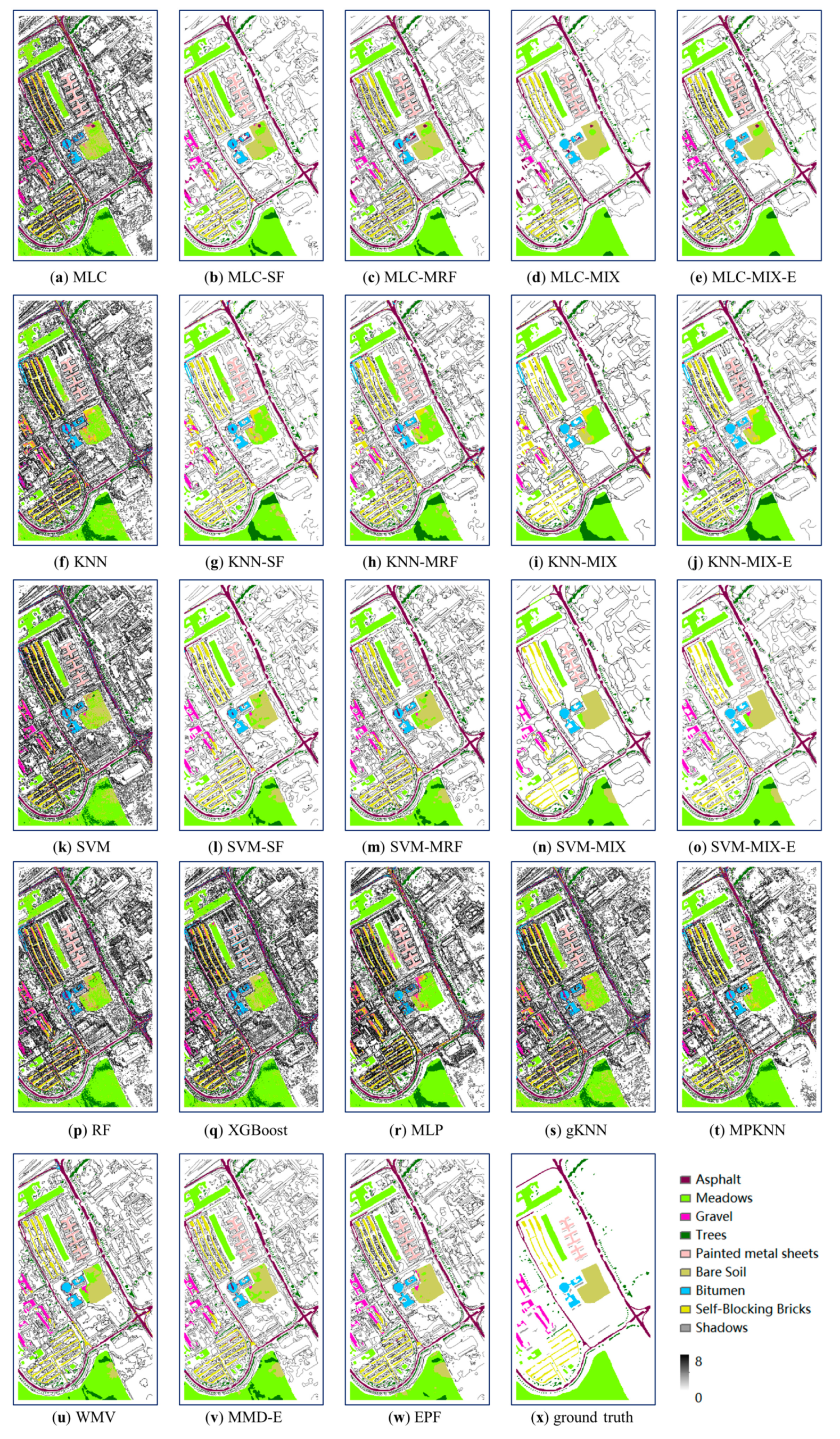
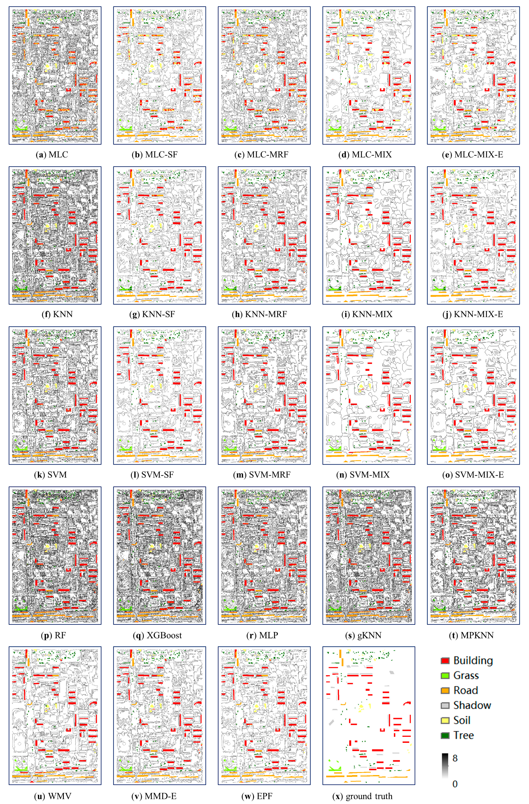
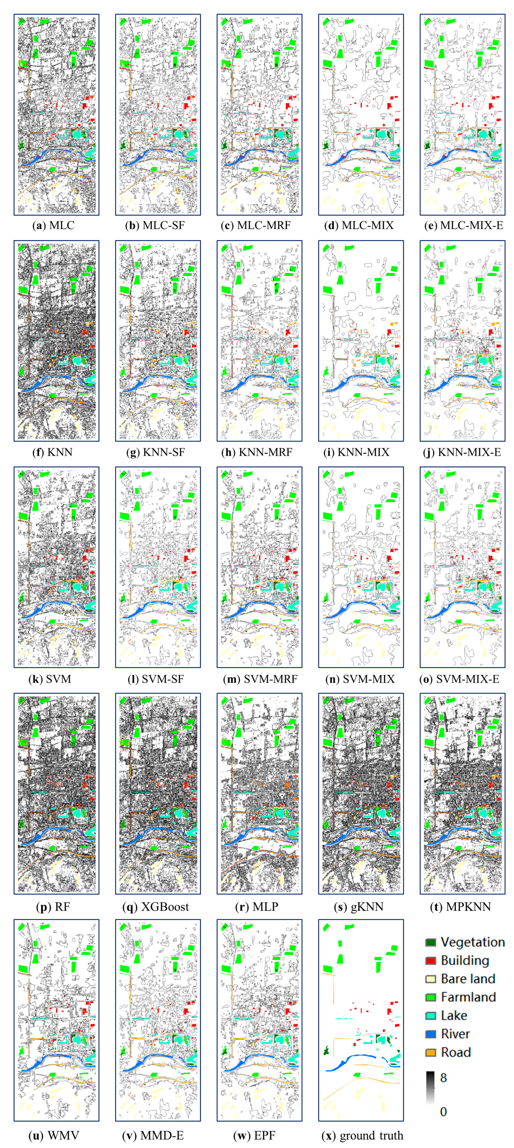
The classification results at ground-truth locations are shown in Figure 4, Figure 5 and Figure 6. Each classification result is superimposed on top of an edge map, which reflects the smoothness of the classification result. The edge map is produced by assigning to each pixel the number of neighboring labels different from that of the central pixel based on the 8-connectivity [53] for the entire classification result. The highest value for a pixel is 8 in the edge map, indicating the pixel is surrounded by pixels with different classes (most likely noise); the lowest value is 0, indicating the pixel has the same class with all its eight neighbors. Since the ground-truth data for entire study areas are not available, there is no reference edge map.

As expected, the classification results largely depend on the initial classifier. For example, in the ROSIS image, bare soils were misclassified as meadows using the KNN classifier (Figure 4f), thus the four KNN enhanced methods (KNN-SF, KNN-MRF, KNN-MIX, and KNN-MIX-E in Figure 4g–j), and the two state-of-the-art methods (gKNN and MPKNN in Figure 4s,t) all suffer from similar misclassifications. Again, for the Landsat image, more buildings appeared in the traditional MLC (Figure 6a) than in the KNN classification (Figure 6f), thus similar trends are observed in the four MLC enhanced methods (SF, MRF, MIX, and MIX-E in Figure 6b–e).

Although all the contextual classification methods can filter noise, employing only one type of context may still cause the results to suffer from this problem. For example, the SF post-classification and MRF methods filter considerable noise from the original classification results, but it still persisted in many places (Figure 4b,c,g,h,l,m). The utilization of spatial pattern and spatial covariance does further smooth noise. For example, the meadows in the ROSIS image are nicely smoothed using the MIX model with all three classifiers (Figure 4d,e,i,j,n,o), but many results using this model suffer from over-smoothing according to the edge maps. The edge constraint capability within the MIX-E model can counter this. For example, the KNN-MIX and SVM-MIX methods fail to keep the connectivity of the asphalts in the ROSIS image in the upper left corner (Figure 4i,n), but by incorporating an edge-preserving filter, the MIX-E model (Figure 4j,o) is able to generate more satisfactory classification results than both the traditional classifiers and the enhanced methods.

Among the eight state-of-the-art methods, the MLP and the MPKNN results (Figure 4r,t, Figure 5r,t and Figure 6r,t) are smoother than the RF, XGBoost, and gKNN results (Figure 4p,q,s, Figure 5p,q,s and Figure 6p,q,s), but all the above five results contain a great deal of noise. Further, linear objects, such as roads in the Landsat image in the lower left corner, are retained only by the classifiers without considering contexts (e.g., MLP in Figure 6r) or those incorporating a single simple context (e.g., MLC-SF, gKNN in Figure 6b,s) at the expense of persistent noise. The edge information is better preserved in the WMV results than with methods reliant on edge preserving filters since the method is object-based, but it still does not do a good job of classifying road objects in the Landsat image because it ignores the contexts between segments. As with MRF, the MMD-E results still retain some noise (Figure 4v, Figure 5v and Figure 6v). The EPF results are well balanced between noise smoothing and detail retention (Figure 4w, Figure 5w and Figure 6w), although a few rough edges appear in the edge maps.

To provide a quantitative assessment, the overall classification accuracy and F1-score of each class were calculated. The McNemar test was performed to test if the increases in overall accuracy (measured as the percentage point change in the percent of correctly classified pixels) of the MIX-E method against other methods are significant at the 99% confidence interval (χ² > 6.63). The enhanced and the state-of-the-art methods were compared with the MIX-E model based on the same classifier. For example, the gKNN and MPKNN were compared with the KNN-MIX-E method, the WMV, MMD-E, and EPF were compared with the SVM-MIX-E method. Since the MIX-E model was not tested on the decision tree and ANN classifiers, the RF, XGBoost, and MLP methods were compared with all three MIX-E classification methods. In addition, the edge preserving ability of classifiers was measured by an edge index, calculated as the mean value of the edge map. The greater the edge index, the noisier the classification result. A too small edge index often suggests an over-smoothed classification result. The classification quality for three study areas is shown in

Table 2. Overall accuracy (%), F1-score per class, and edge index of classification results for the ROSIS dataset.

Classifier	Algorithm	Edge	Accuracy
			Total	1	2	3	4	5	6	7	8	9
MLC	MLC	2.6	83.0 *	0.89	0.67	0.8	0.65	0.87	0.99	0.81	0.99	0.76
	SF	0.8	90.7 *	0.94	0.84	0.89	0.82	0.93	0.99	0.91	0.97	0.8
	MRF	1.1	90.5 *	0.92	0.86	0.83	0.81	0.93	1	0.9	0.99	0.8
	MIX	0.6	92.9 *	0.93	0.89	0.95	0.71	0.96	1	0.92	0.96	0.87
	MIX-E	0.9	94.0	0.96	0.89	0.99	0.84	0.96	1	0.96	1	0.87
KNN	KNN	2.7	71.3 †	0.8	0.33	0.59	0.43	0.79	0.97	0.71	1	0.69
	SF	0.9	77.7 †	0.93	0.31	0.85	0.63	0.82	0.98	0.78	0.97	0.66
	MRF	1.0	76.8 †	0.92	0.27	0.79	0.55	0.82	0.98	0.76	1	0.69
	MIX	0.6	78.7 †	0.93	0.3	0.88	0.56	0.84	1	0.76	0.97	0.65
	MIX-E	0.9	80.1	0.94	0.31	0.87	0.66	0.85	0.98	0.78	0.99	0.69
SVM	SVM	2.8	81.3 #	0.86	0.64	0.66	0.72	0.86	0.99	0.83	1	0.77
	SF	0.9	90.2 #	0.97	0.78	0.96	0.9	0.91	1	0.93	0.98	0.8
	MRF	1.0	89.6 #	0.96	0.78	0.91	0.88	0.9	1	0.92	1	0.81
	MIX	0.4	93.3 #	0.97	0.89	0.99	0.93	0.94	1	0.95	0.96	0.83
	MIX-E	0.7	93.8	0.98	0.89	1	0.9	0.95	1	0.94	0.99	0.85
State-of-the-art methods	RF	2.8	77.5 *,†	0.83	0.52	0.62	0.57	0.84	1	0.77	0.93	0.71
	XGBoost	3.0	75.8 *,†,#	0.81	0.5	0.55	0.56	0.83	0.83	0.77	0.99	0.72
	MLP	2.6	71.1 *,†,#	0.71	0.33	0.57	0.05	0.84	0.98	0.6	0.9	0.75
	gKNN	2.8	71.4 †	0.81	0.35	0.6	0.5	0.78	0.97	0.72	1	0.7
	MPKNN	2.1	78.2 †	0.87	0.26	0.73	0.58	0.84	0.98	0.77	0.99	0.74
	WMV	1.1	89.3 #	0.94	0.76	0.93	0.91	0.91	0.98	0.9	0.93	0.81
	MMD-E	1.1	90.0 #	0.97	0.79	0.92	0.88	0.91	1	0.92	1	0.81
	EPF	1.1	93.0 #	0.98	0.83	0.99	0.88	0.94	1	0.94	1	0.91

Class: 1–Asphalt, 2–Bare soil, 3–Bitumen, 4–Gravel, 5–Meadows, 6–Painted metal sheets, 7–Self–blocking bricks, 8–Shadows, 9–Trees. * Significant when comparing with the MLC-MIX-E, ^† significant when comparing with the KNN-MIX-E, ^# significant when comparing with the SVM-MIX-E.

,

Table 3. Overall accuracy (%), F1-score per class, and edge index of classification results for the IKONOS dataset.

Classifier	Algorithm	Edge	Accuracy
			Total	1	2	3	4	5	6
MLC	MLC	1.9	76.0 *	0.69	0.86	0.8	0.98	0.38	0.94
	SF	0.8	81.0 *	0.75	0.94	0.86	0.99	0.43	0.97
	MRF	1.0	80.5 *	0.75	0.91	0.84	0.99	0.44	0.96
	MIX	0.6	82.2 *	0.77	0.94	0.88	0.99	0.44	0.96
	MIX-E	0.8	83.5	0.79	0.96	0.88	0.99	0.46	0.97
KNN	KNN	2.3	88.7 †	0.91	0.65	0.82	0.99	0.83	0.88
	SF	0.8	93.4 †	0.95	0.65	0.9	1	0.93	0.9
	MRF	0.9	93.4 †	0.95	0.77	0.89	1	0.89	0.93
	MIX	0.4	93.6 †	0.95	0.72	0.91	0.98	0.96	0.92
	MIX-E	0.7	95.2	0.96	0.81	0.92	1	0.94	0.94
SVM	SVM	1.7	91.7 #	0.93	0.87	0.85	0.99	0.84	0.95
	SF	0.7	94.4 #	0.94	0.93	0.89	1	0.9	0.97
	MRF	0.7	93.7 #	0.94	0.91	0.88	1	0.88	0.97
	MIX	0.3	93.3 #	0.93	0.98	0.88	0.96	0.9	0.99
	MIX-E	0.4	95.4	0.95	0.98	0.91	1	0.91	0.99
State-of-the-art methods	RF	2.5	88.7 †,#	0.91	0.72	0.81	0.98	0.81	0.88
	XGBoost	2.5	87.9 †,#	0.9	0.74	0.81	0.98	0.76	0.89
	MLP	2.0	89.0 †,#	0.91	0.75	0.84	0.97	0.77	0.89
	gKNN	2.3	88.5 †	0.9	0.69	0.81	0.99	0.8	0.89
	MPKNN	1.9	92.9 †	0.95	0.7	0.9	0.98	0.92	0.9
	WMV	0.8	93.1 #	0.93	0.99	0.84	0.99	0.92	0.97
	MMD-E	0.8	93.9 #	0.94	0.9	0.89	1	0.87	0.97
	EPF	0.8	95.8	0.96	0.96	0.92	1	0.94	0.99

Class: 1–Building, 2–Grass, 3–Road, 4–Shadow, 5–Soil, 6–Tree. * Significant when comparing with the MLC-MIX-E, ^† significant when comparing with the KNN-MIX-E, ^# significant when comparing with the SVM-MIX-E.

and

Table 4. Overall accuracy (%), F1-score per class, and edge index of classification results for the Landsat dataset.

Classifier	Algorithm	Edge	Accuracy
			Total	1	2	3	4	5	6	7
MLC	MLC	1.9	87.7 *	0.93	0.8	0.89	0.99	0.95	0.84	0.61
	SF	1.2	90.4 *	0.94	0.83	0.92	0.99	0.96	0.85	0.66
	MRF	0.7	90.5 *	0.93	0.82	0.93	0.99	0.95	0.84	0.69
	MIX	0.4	92.3 *	0.97	0.76	0.98	0.96	0.94	0.79	0.87
	MIX-E	0.5	94.7	0.96	0.86	0.98	0.98	0.97	0.86	0.87
KNN	KNN	2.7	81.9 †	0.86	0.59	0.87	1	1	0.67	0.25
	SF	1.4	84.6 †	0.87	0.57	0.9	1	1	0.7	0.18
	MRF	0.7	84.3 †	0.9	0.58	0.9	1	1	0.65	0.19
	MIX	0.3	85.4 †	0.97	0.58	0.92	0.98	1	0.61	0.26
	MIX-E	0.5	87.4	0.96	0.7	0.91	1	1	0.7	0.26
SVM	SVM	1.7	89.5 #	0.9	0.87	0.92	1	1	0.82	0.55
	SF	0.7	92.0 #	0.94	0.93	0.93	1	1	0.88	0.55
	MRF	0.6	92.5 #	0.93	0.93	0.93	1	1	0.89	0.57
	MIX	0.4	92.1 #	0.97	0.93	0.94	0.97	1	0.81	0.6
	MIX-E	0.5	93.3	0.96	0.95	0.94	1	1	0.88	0.58
State-of-the-art methods	RF	2.9	82.5 *,†,#	0.88	0.67	0.84	1	1	0.69	0.4
	XGBoost	2.9	83.5 *,†,#	0.87	0.73	0.85	0.99	0.99	0.7	0.41
	MLP	2.0	82.1 *,†,#	0.92	0.53	0.89	0.98	0.96	0.6	0.04
	gKNN	2.8	81.4 †	0.87	0.59	0.85	1	1	0.65	0.28
	MPKNN	2.2	85.2 †	0.88	0.61	0.91	1	1	0.66	0.21
	WMV	0.7	93.2	0.94	0.93	0.94	0.99	1	0.9	0.58
	MMD-E	0.6	92.4 #	0.93	0.93	0.93	1	1	0.89	0.55
	EPF	0.8	92.6 #	0.92	0.9	0.94	1	1	0.87	0.66

Class: 1–Bare land, 2–Building, 3–Farmland, 4–Lake, 5–River, 6–Road, 7–Vegetation. * Significant when comparing with the MLC-MIX-E, ^† significant when comparing with the KNN-MIX-E, ^# significant when comparing with the SVM-MIX-E.

.

The edge index greater than 2 usually indicates a noisy classification result without consideration of neighborhood contexts, as revealed by edge maps in Figure 4, Figure 5 and Figure 6. The edge index in Table 2, Table 3 and Table 4 is around or below 1 in most contextual classifications. The value smaller than 0.5 corresponds to an over-smoothed result (the MIX method) and hence a reduced accuracy.

The overall classification accuracies show that all the enhanced methods improve classification accuracies over their original counterparts, but the original classifier itself has a great impact on the final accuracy. The improvement over the enhanced MRF and SF is relatively similar for both methods. The MIX-E model is also consistently more accurate than the MIX, indicating that the edge preserving filter improves classification accuracy. The improvement is relatively small because MIX itself incorporates elements of spatial context, nevertheless it is statistically significant. Regardless of which classifier is applied, the MIX-E model developed here outperforms the original classifiers and the three enhanced methods in classification accuracy for all three cases.

For the state-of-the-art methods, the decision tree based methods (RF and XGBoost) outperform the MLP in the ROSIS image. The RF, XGBoost, and MLP methods outperform all the MLC enhanced methods in the case of the IKONOS image due to a relative low accuracy for the traditional MLC method. However, the accuracies for the MIX-E model based on KNN and SVM are significantly higher than those for these three methods (RF, XGBoost, and MLP) that do not consider contexts. The accuracies for MPKNN are higher than those for gKNN, indicating the spatial pattern derived from MP probability improves the classification accuracy. Accuracies relative to the MMD-E and MRF methods are also relatively similar. This suggests that an edge preserving filter does not show a great advantage if only one context (i.e., the neighborhood context from MRF) is considered. Only the EPF method in this case betters our new method. Even so, its overall accuracy is only 0.4 of a percentage point higher than the MIX-E method. Other than for EPF, the only non-statistically significant improvement in accuracy was relative to WMV for the Landsat data. As an OBIA, it was particularly adept at capturing the narrow spatial shape of roads and crossroads in this image, as evidenced by its high overall accuracy score (93.2%) in Table 4. The increases in accuracy using the MIX-E model are significant at the 99% confidence level in all other cases.

According to the F1-score, misclassification is often caused by similar spectral features of different classes, for example, the gravel and bare soil classes in the ROSIS image. One reason that limits the increase in accuracy using the contextual methods is the low accuracy of some classes derived from the traditional classifier. Another important factor that affects contextual classifications is the proportion of this class within a range. A typical case is the bare soil class in the ROSIS image has low F1-scores using all the three traditional classifiers (MLC, KNN, and SVM). The MIX-E model improves its F1-score from 0.67 to 0.89 and 0.64 to 0.89 based on the MLC and SVM classifiers, respectively. However, the KNN-MIX-E method reduces its F1-score from 0.33 to 0.31 because the bare soil class is not the dominant class within a certain range (in the middle of the study area), and it is thus filtered out when incorporating contexts.

3.2. Parameter Analysis

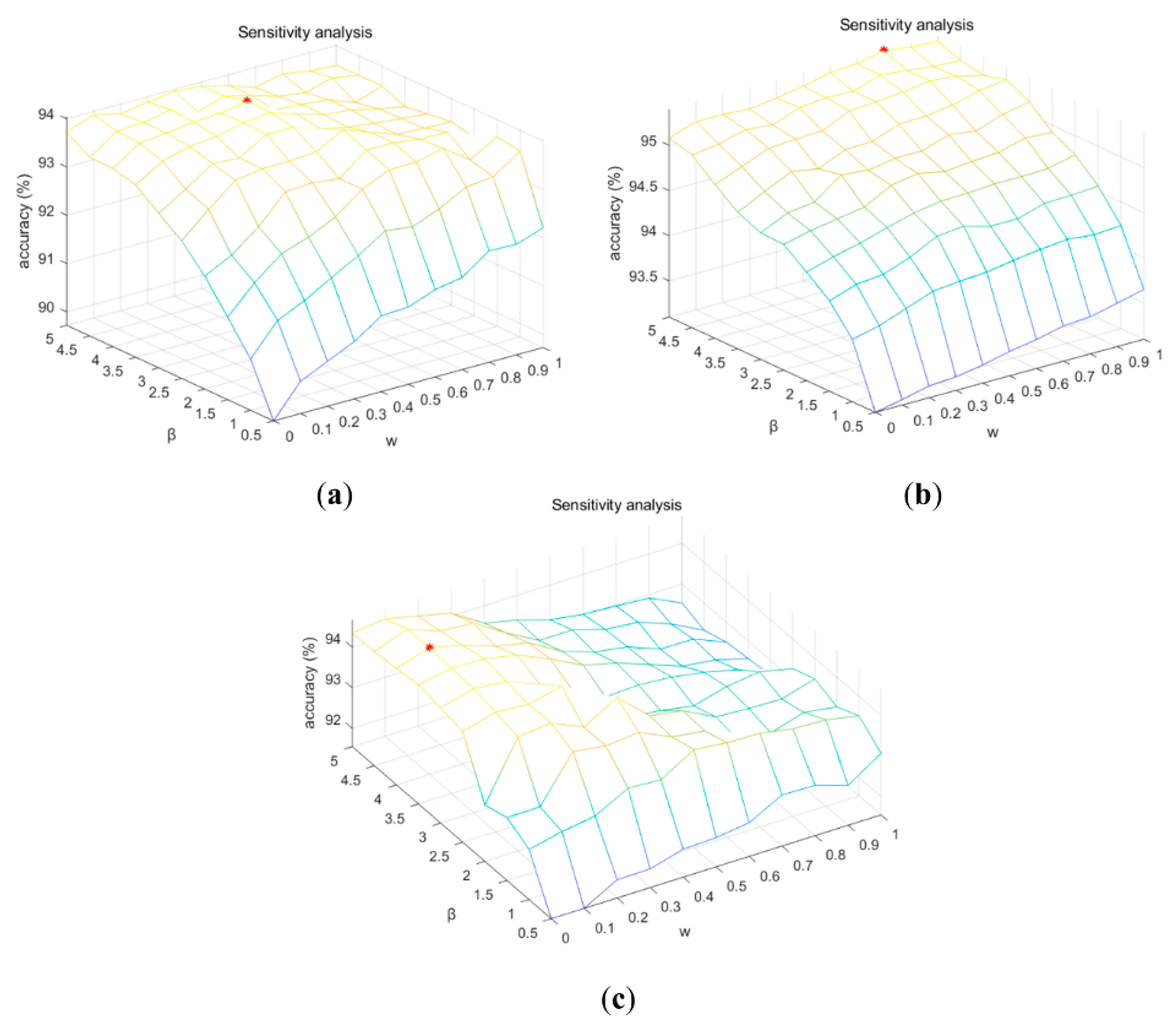
There are several parameters in the developed method that can affect classification results, specifically the proportional weighting, w, the edge-preserving parameter, α, and the smoothing parameter, β, in Equation (8), as well as the decrease rate and the convergence parameter in MRF. Many prior studies have used predetermined and fixed parameters [41,54] because the automatic selection of parameters is challenging [55]. It is beyond the scope of the current paper to analyze the impact of all the parameters, therefore most parameters were not customized here. For example, simply the mean value of gradients was used for the edge-preserving parameter, α, which limits the impact of contexts from the lowest value of 0.008 near edges to the highest value of 0.962 far away from edges. Rather, we focused on the choices of the proportional weighting, w, and the smoothing parameter, β. The former decides the balance between spatial pattern and spatial correlation, and is a new parameter introduced with the MIX-E model. The latter controls the smoothness of results. Of special interest is whether the choice of β in the MIX-E model has a different impact than in traditional MRF methods. Parameter sensitivity was explored with weight w varying from 0 to 1 in intervals of 0.1, and β from 0.5 to 5 in intervals of 0.5, resulting in 110 combinations in total. Figure 7 shows the overall classification accuracies against varying proportional weighting, w, and smoothing parameter, β, values, with the maximum values marked by red stars. Only the classifiers using the MIX-E model with the greatest accuracy are shown for each dataset.

As can be seen from Figure 7, initial increases in the smoothing parameter, β, lead to higher accuracy in all three cases. Accuracy reaches a maximum and then decreases slightly as β increases for the ROSIS and Landsat cases, but it keeps increasing for the IKONOS dataset. However, the classification result becomes over-smoothed when β exceeds 5 for the IKONOS dataset due to its relatively simple class distribution. Therefore, we stopped when β equaled 5. All three cases indicate that the choice of a small value for the smoothing parameter, β, is not recommended, as in the traditional MRF methods, because the extra smoothness caused by spatial pattern and spatial correlation can be counterbalanced by the edge information.

As the proportional weighting, w, increases, spatial pattern gains more weight relative to spatial correlation. When β is large, the classification accuracies are relatively high, with w varying from 0.2 to 0.8 for the ROSIS (Figure 7a) and IKONOS (Figure 7b) cases. In the case of Landsat (Figure 7c), higher accuracies are also achieved when β takes a large value and w a small value. Both observations indicate that the combination of two contexts (spatial pattern and spatial correlation) can improve the classification results over one alone since the highest accuracies are achieved when w is neither 0 nor 1.

3.3. Spatial Pattern vs. Spatial Correlation

The MIX-E model merges MPG and spatial covariance into its MRF optimization, thus incorporating contexts representing spatial pattern and spatial correlation, respectively. As mentioned before, spatial pattern characterizes the degree of aggregation of land cover patterns at the global level and is an isotropic measure. Spatial correlation, on the other hand, measures pairwise spatial correlation in each individual direction, and characterizes the distribution of a class at the local level.

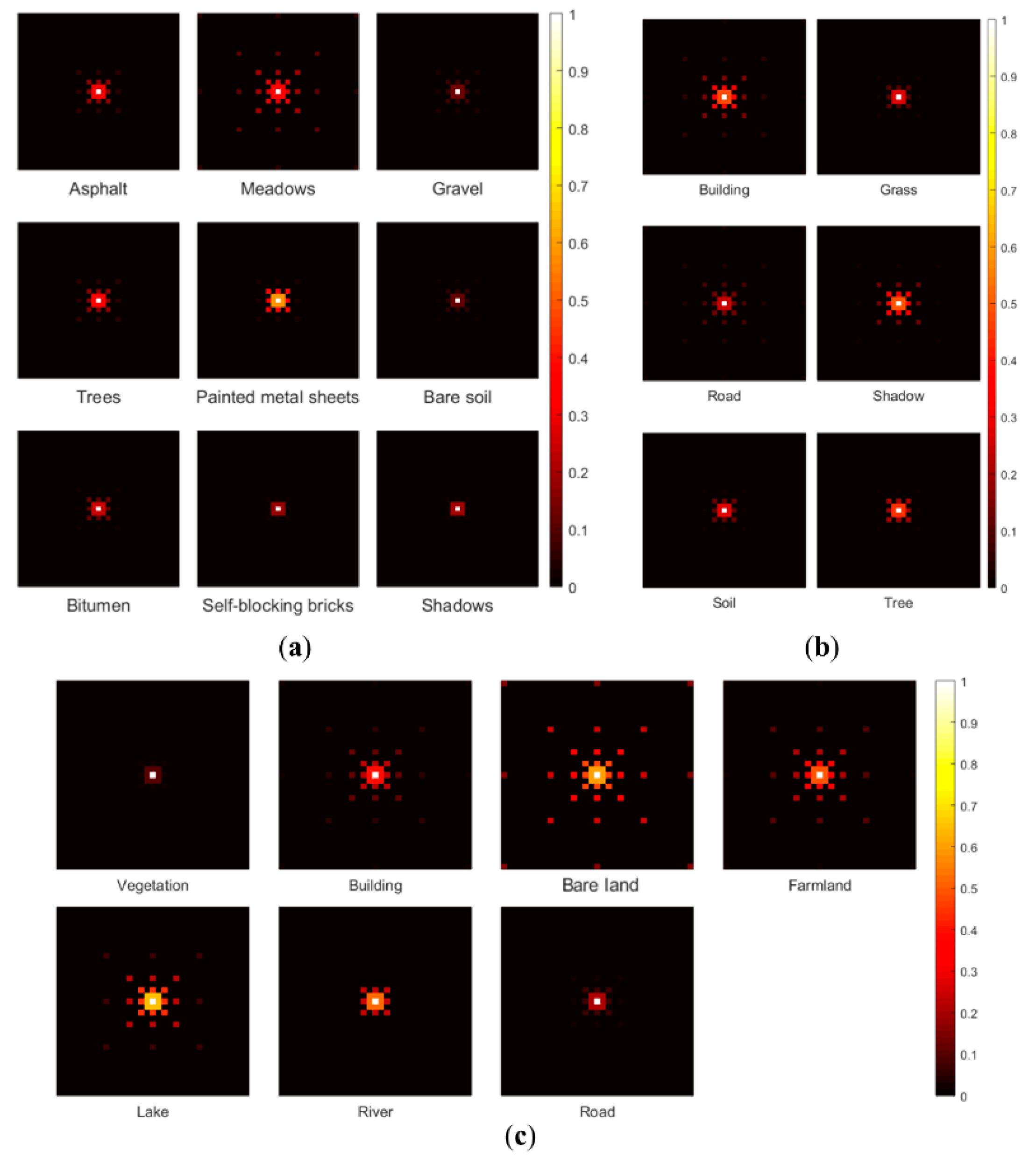
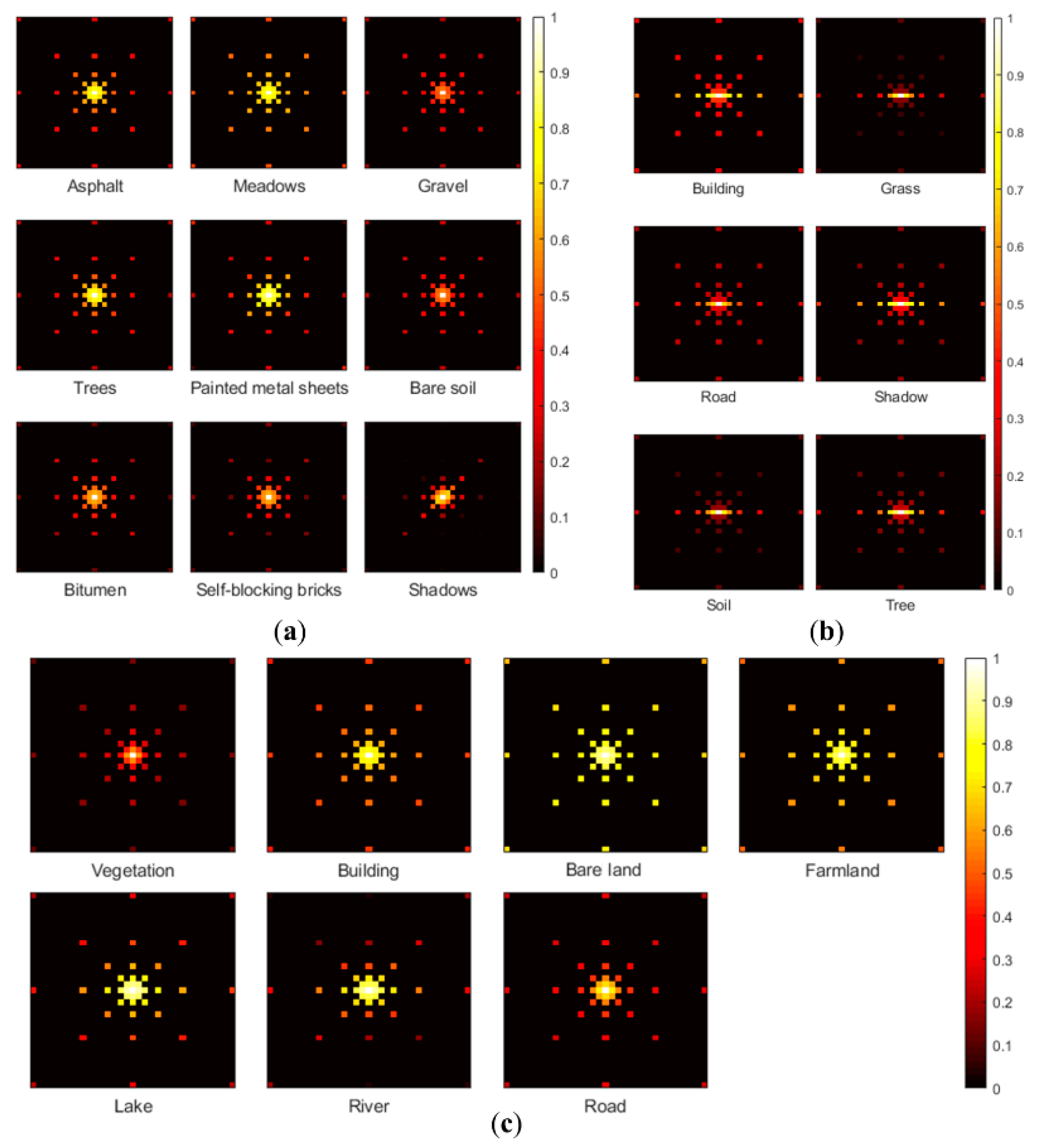
The spatial patterns and spatial correlations were derived from the initial classification results using a 3 × 3 data template with a multi-grid level L of 5, which implies five lag intervals. They were computed in all eight cardinal directions (south, north, east, west, southeast, southwest, northeast, northwest), as illustrated in Figure 3. The MLC results was used as an example of the extraction of spatial contexts. Figure 8 and Figure 9 show the spatial pattern and spatial correlation of classes from the multi-grid data template illustrated in Figure 3. The patterns in Figure 8 reflect the spatial distribution of land cover classes, with more spatially concentrated classes having a large MP probability. For example, the lake class in the Landsat image, although not the dominant class, has a pattern that is clustered in patches, leading to a larger MP probability. The spatial correlation in Figure 9 is related to lag distance, with pixels separated by smaller distances having greater spatial correlation than those separated by larger distances. Some classes show anisotropic correlation. For example, all six classes in the IKONOS image show stronger correlations in the horizontal direction, indicating the classes are distributed more continuously horizontally.

However, how spatial pattern and spatial correlation affected the classification is not obvious from Figure 8 and Figure 9. Therefore, we further evaluated their specific contribution to the classification results by applying these two contexts individually to the ROSIS and Landsat datasets. The IKONOS image was not included due to its relatively simple land cover distribution. Since edge information was not considered, the gradient ρ(u_i) in Equation (8) was set to 0. To isolate the individual contribution of each spatial context to the classification result, w was set to 0 for spatial correlation only and to 1 for spatial pattern only. Since we focused on the pattern distribution of land cover classes rather than classification accuracy, the entire classification results are shown in Figure 10 and Figure 11, along with zoomed views of a portion of the results.

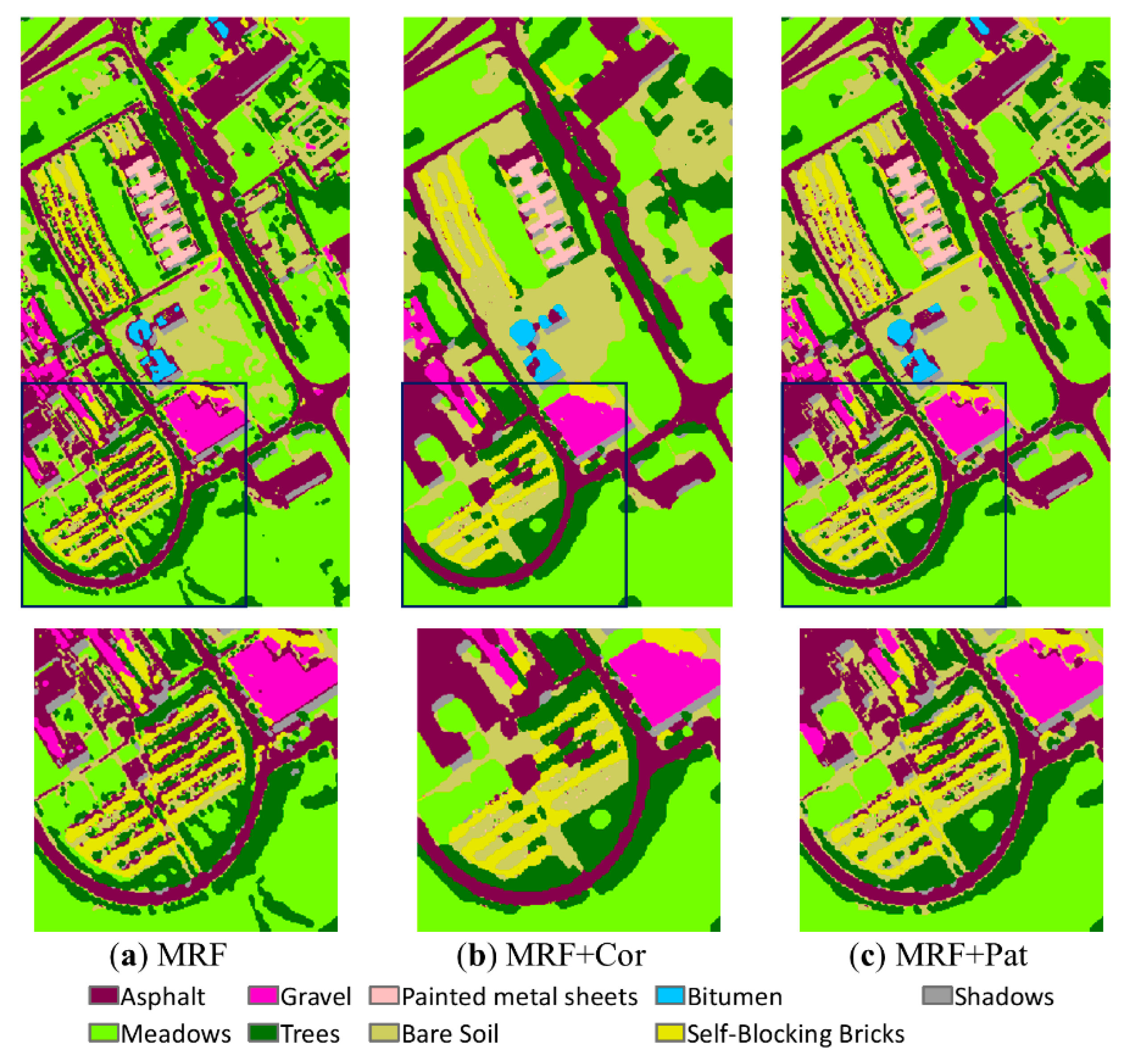
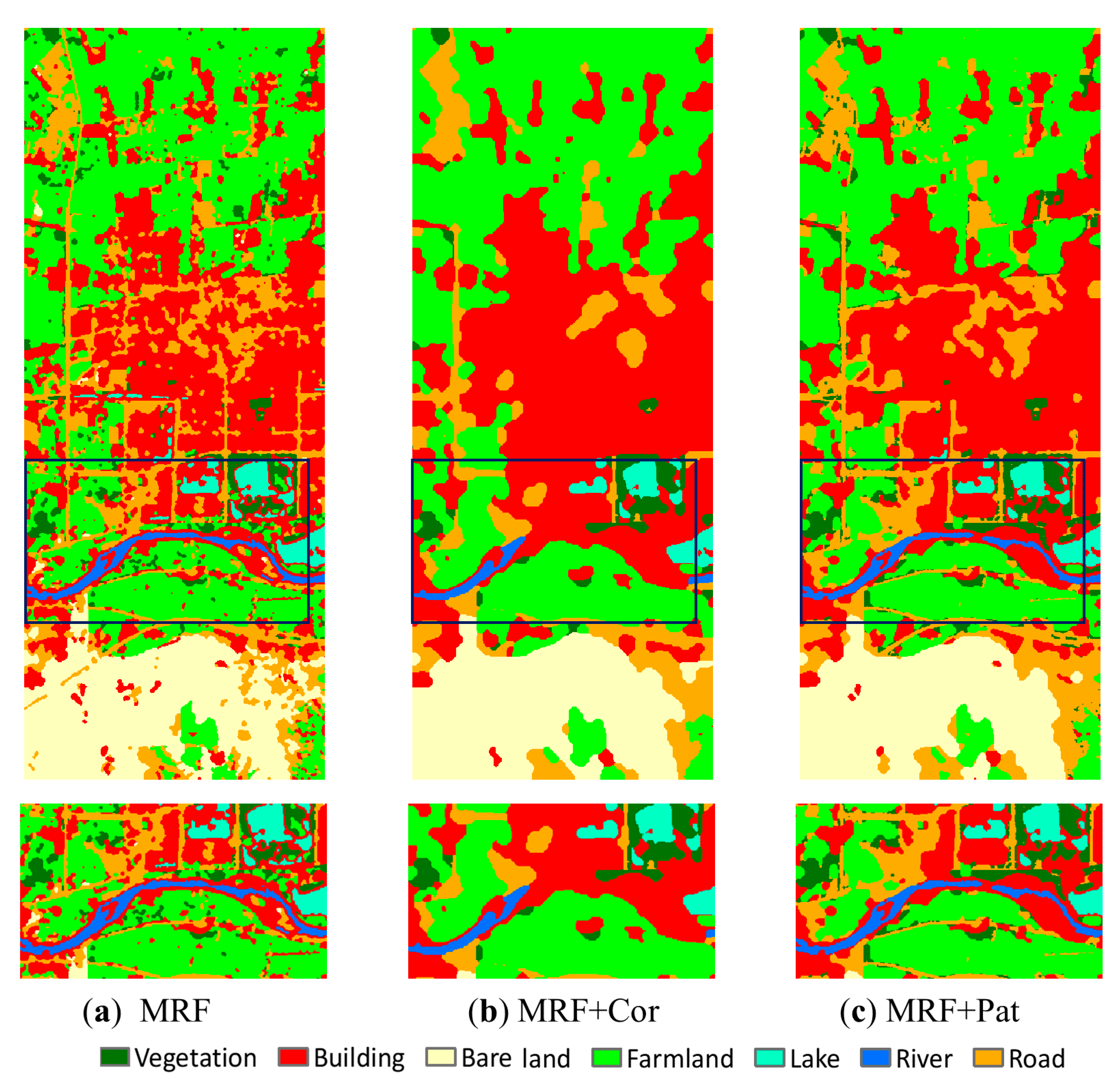
Combining either of the contexts (spatial pattern or spatial correlation) with MRF generates smoother results compared with MRF alone, but results for MRF combined with spatial correlation (MRF + Cor) are smoother than for MRF combined with spatial pattern (MRF + Pat). Spatial pattern is more capable of capturing linear and curvilinear objects, which are more interrupted using spatial correlation, effects which are apparent in asphalt in the ROSIS image and road and river in the Landsat image. However, some noise is also produced, for example, in the upper right corner of the zoomed image in Figure 10c for the gravel class. Spatial pattern appears to produce replications of this class in all the directions within a data template. Overall, due to its capability for characterizing joint relationships, spatial pattern can smooth results without losing linear/curvilinear details, but at the expense of increasing noise near edges, whereas spatial correlation produces a smoother result due to its additive anisotropic effects, but it may compromise the connectivity of patterns.

4. Discussion

A key feature of our MIX-E model is the incorporation of spatial contexts, but the initial extraction of these contexts requires prior knowledge. Hence, it is important to examine the potential impact of this prior knowledge on model performance, as well as other more general limitations and challenges of the MIX-E model.

4.1. Training Image Selection

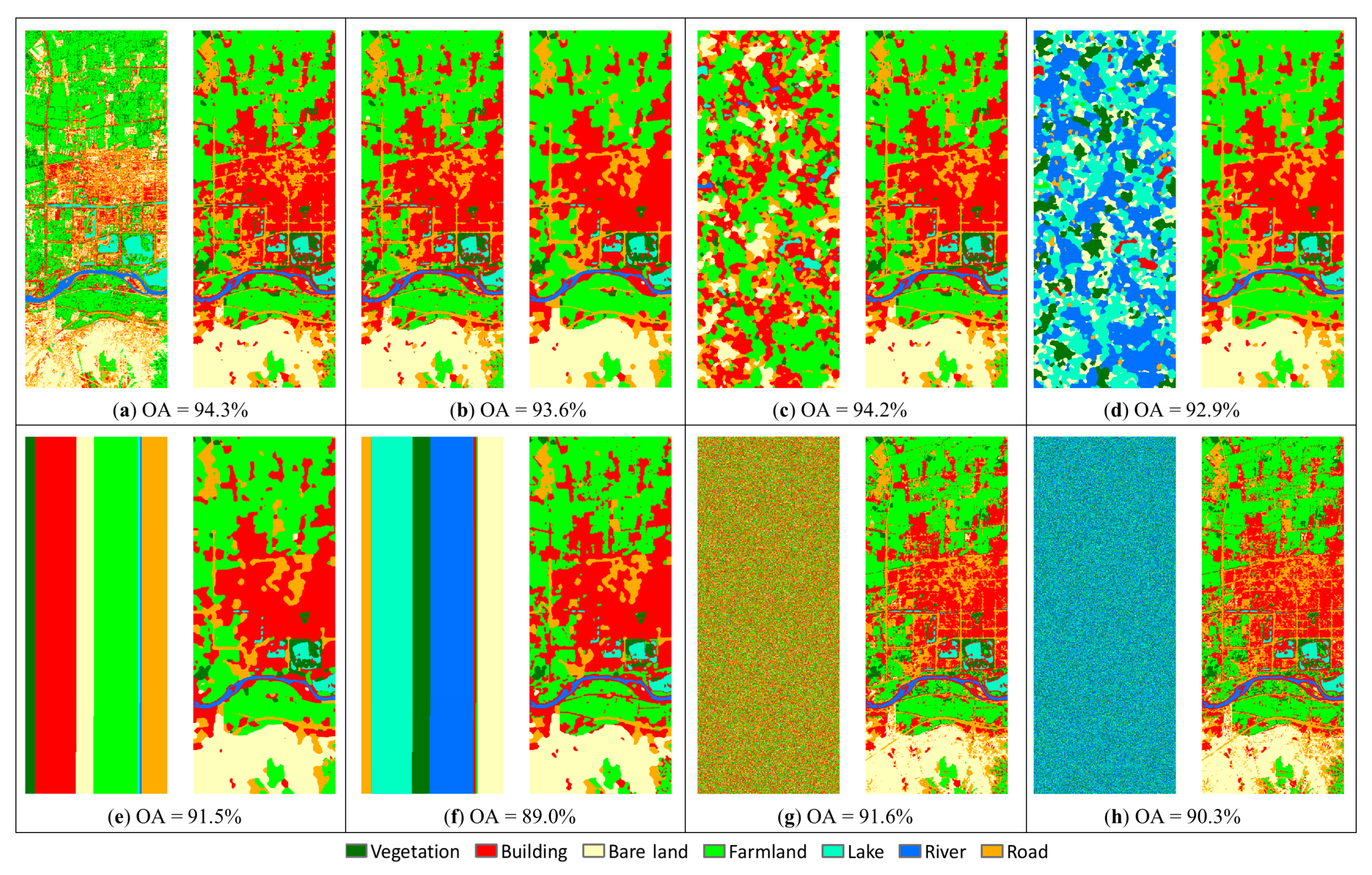
A training image (TI) is used as the prior knowledge for extracting spatial pattern and spatial correlation contexts. How might imperfect or defective TIs affect the classification results? The classification method for producing a TI can be different from that of the classifier employed by the main model, although we used the same method. Further, the TI does not even need to be derived from a classification result or from an image of the same size. In the following analysis of the potential impact of different TIs, for simplicity, only the Landsat dataset was used and only the MIX-E model based on the MLC classifier was considered since it has the highest accuracy (94.7%). Eight different images were used as TIs for comparison. The TIs and corresponding classification results are shown in Figure 12, along with the reported overall accuracies (OA). The first TI (Figure 12a) is the KNN classification result, which allows us to check how an inaccurate TI affects the classification result since the accuracy of the KNN (81.9%) is lower than that of the MLC (87.7%). As a contrast, the MLC-MIX-E result itself is taken as a TI (Figure 12b) to check if the classification result can be further improved using a TI with high accuracy. The third and fourth TIs are two simulated images created using single normal equation simulation (SNESIM) [56]; one has similar class proportions (i.e., proper proportions) to the classification result (about 7% vegetation, 29% building, 12% bare land, 31% farmland, 2% lake, 1% river, and 18% road classes) (Figure 12c), while the other has the same pattern but with very different class proportions (i.e., improper proportions) (Figure 12d). The last four TIs are artificial image patterns of vertical stripes (Figure 12e,f) and random noise (Figure 12g,h). Both stripes and noise patterns include two scenarios: Similar class proportions to the classification result (i.e., proper proportions) and very different class proportions (i.e., improper proportions). The TIs with stripes pattern have very good MP probabilities for the classes with large proportions and high spatial correlation in the north and south directions. The TIs with random noise have zero MP probabilities and similar spatial correlation in each direction. All other parameters were set the same as those used in the MLC-MIX-E method.

Interestingly, the MLC-MIX-E has a higher accuracy (94.7%) than that of the KNN (81.9%) but the classification using the former as the TI leads to a lower accuracy (93.6%) than that using the latter (94.3%). This occurs because the MLC-MIX-E itself is a smoothed result, and therefore some details are not retained when an over-smoothed image is used as the TI. Also notable is that the class distribution of the classification map using the KNN result as the TI is more similar to the MLC result (more buildings) than that of the KNN result (less buildings), indicating that the classifier rather than the TI is decisive to the final classification. The accuracies achieved using the two simulated images as TIs (94.2% for the proper and 92.9% for the improper class distributions) further proves that a high accuracy TI is not required, but proper class proportion is helpful. The classification accuracies are relatively low using all the stripes and random noise patterns as TIs. However, again, TIs with proper class proportions lead to higher accuracies than those with improper class proportions. The stripes patterns lead to smoother classification results than those of the noise patterns, so the contexts derived from TIs with stripes pattern have a greater influence than those with noise patterns. Not unexpectedly, the classification accuracies using the TIs with stripes patterns are lower than for the first four TIs because misleading contexts are provided. Similarly, the classification result based on the random noise pattern with improper class proportions as the TI has more noise than that with proper class proportions since there are no useful contexts extracted from the former.

Overall, these tests demonstrate that similar class distributions and proportions to the underlying scene are preferred when choosing appropriate TIs, but an imperfect TI is still acceptable because the classifier plays the decisive role. The test also demonstrates the advantage of the developed method for integrating contexts into an MRF framework. The MRF is an optimization algorithm, and a relatively stable result can be achieved by its iterative updating of the energy function. If the TI does not provide any useful contexts, such as in the case of random noise with improper class proportions (Figure 12h), the MIX-E model is basically degraded to a simple MRF model with no consideration of other contexts.

4.2. Pros and Cons

The model developed here outperformed most classification methods we tested using the experimental data. It provides a solution for integrating different types of contexts derived from both the original image and its initial classification results. The model is suited to different types of remote sensing datasets and many probabilistic classification methods. It infers spatial correlation contexts directly from TIs rather than from sample data, thus avoiding the involvement of expert knowledge in determining initial parameters during the modeling process. Another advantage of introducing TIs is that the choice of sampling schemes can be avoided. In previous methods, such as gKNN and MPKNN, the autocorrelation in the sampling data needs to be considered in order to establish a proper model.

The spatial pattern and spatial correlation in this method are both based on indicator functions, deriving contexts by counting occurrences of classes. There are other types of contexts, for example, local indicators of spatial association (LISA) [57], join count statistics (JCSs) [58,59], and geographic connectivity matrices [5]. However, some contexts are only suited to specific classifiers. Basically, the locational information, the method for combining spatial and spectral information, and the applicability to massively large datasets should be considered together in order to construct a contextual classification method. Recently, Huang et al. [14] proposed a relearning method to iteratively update the initial classification result according to the frequency and spatial pattern of the class labels. The deep learning technology emerging nowadays, such as convolutional neural networks (CNNs), has been used for remote sensing classification [60,61] and can achieve very high classification accuracy. Both aspects are very promising and may be applied to the MIX-E model. However, the MIX-E model is established by scanning the TI once only at a single grid level, without iteratively learning the contexts. The application of relearning techniques may require model modifications in order to reduce the computational load. The CNN method extracts abstract features from a large amount of image patches. In order to apply it to the MIX-E model, contexts between image patches instead of pixels should be considered. Also, new schemes for combining all the features instead of the current proportional weighting scheme may be required. How to integrate contexts into non-probabilistic classifiers (e.g., the decision tree classifier) is also worth further exploration.

5. Conclusions

This paper developed a new contextual classification method based on the MIX-E model. The model includes two complimentary contexts: Spatial pattern and spatial correlation, both of which lead to smoothing effects. The former characterizes the degree of aggregation of land cover classes and is able to retain linear/curvilinear features, whereas the latter quantifies pairwise correlation by assigning anisotropic weighting in various distances and directions. The combination of these two contexts can improve the classification result over the use of one alone. Additionally, an edge-preserving filter was applied to prevent an over-smoothed result. All the contexts were integrated into a higher-order multi-grid MRF framework, which makes it possible for a relatively stable result to be obtained through optimization. The integration of different contexts over a long-was is superior to the traditional MRF method, which is based on an isotropic, nearest neighborhood context alone. The developed model was tested with three commonly used probabilistic classifiers using three different data sources with differing land cover characteristics. The new method was shown to increase classification accuracy significantly compared with other enhanced contextual methods and most state-of-the-art classification methods.

References

- Shekhar, S.; Schrater, P.; Vatsavai, R.R.; Weili, W.; Chawla, S. Spatial contextual classification and prediction models for mining geospatial data. IEEE Trans. Multimedia 2002, 4, 174–188. [Google Scholar] [CrossRef]
- Osaku, D.; Nakamura, R.Y.M.; Pereira, L.A.M.; Pisani, R.J.; Levada, A.L.M.; Cappabianco, F.A.M.; Falcão, A.X.; Papa, J.P. Improving land cover classification through contextual-based optimum-path forest. Inf. Sci. 2015, 324, 60–87. [Google Scholar] [CrossRef] [Green Version]
- Tobler, W.R. A computer movie simulating urban growth in the Detroit region. Econ. Geogr. 1970, 46, 234–240. [Google Scholar] [CrossRef]
- Atkinson, P.M.; Lewis, P. Geostatistical classification for remote sensing: An introduction. Comput. Geosci. 2000, 26, 361–371. [Google Scholar] [CrossRef]
- Griffith, D.A.; Fellows, P.L. Pixels and eigenvectors: Classification of Landsat TM imagery using spectral and locational information. In Spatial Accuracy Assessment: Land Information Uncertainty in Natural Resources; CRC: Kim Lowell, Annick Jaton, 2000; pp. 309–317. [Google Scholar]
- Magnussen, S.; Boudewyn, P.; Wulder, M. Contextual classification of Landsat TM images to forest inventory cover types. Int. J. Remote Sens. 2004, 25, 2421–2440. [Google Scholar] [CrossRef]
- Ghimire, B.; Rogan, J.; Miller, J. Contextual land-cover classification: Incorporating spatial dependence in land-cover classification models using random forests and the Getis statistic. Remote Sens. Lett. 2010, 1, 45–54. [Google Scholar] [CrossRef]
- Negri, R.G.; Dutra, L.V.; Sant’Anna, S.J.S. An innovative support vector machine based method for contextual image classification. ISPRS J. Photogramm. Remote Sens. 2014, 87, 241–248. [Google Scholar] [CrossRef]
- Pasolli, E.; Melgani, F.; Tuia, D.; Pacifici, F.; Emery, W.J. SVM active learning approach for image classification using spatial information. IEEE Trans. Geosci. Remote Sens. 2014, 52, 2217–2233. [Google Scholar] [CrossRef]
- Pereira, D.R.; Papa, J.P. A new approach to contextual learning using interval arithmetic and its applications for land-use classification. Pattern Recognit. Lett. 2016, 83, 188–194. [Google Scholar] [CrossRef]
- Ma, L.; Ma, A.; Ju, C.; Li, X. Graph-based semi-supervised learning for spectral-spatial hyperspectral image classification. Pattern Recognit. Lett. 2016, 83, 133–142. [Google Scholar] [CrossRef]
- Zhao, W.; Du, S.; Wang, Q.; Emery, W.J. Contextually guided very-high-resolution imagery classification with semantic segments. ISPRS J. Photogramm. Remote Sens. 2017, 132, 48–60. [Google Scholar] [CrossRef]
- Tang, Y.; Jing, L.; Li, H.; Atkinson, P.M. A multiple-point spatially weighted k-NN method for object-based classification. Int. J. Appl. Earth Obs. Geoinf. 2016, 52, 263–274. [Google Scholar] [CrossRef] [Green Version]
- Huang, X.; Lu, Q.; Zhang, L.; Plaza, A. New postprocessing methods for remote sensing image classification: A systematic study. IEEE Trans. Geosci. Remote Sens. 2014, 52, 7140–7159. [Google Scholar] [CrossRef]
- Wang, L.; Huang, X.; Zheng, C.; Zhang, Y. A Markov random field integrating spectral dissimilarity and class co-occurrence dependency for remote sensing image classification optimization. ISPRS J. Photogramm. Remote Sens. 2017, 128, 223–239. [Google Scholar] [CrossRef]
- Tomasi, C.; Manduchi, R. Bilateral filtering for gray and color images. In Proceedings of the Sixth International Conference on Computer Vision, Bombay, India, 7 January 1998. [Google Scholar]
- Perona, P.; Malik, J. Scale-space and edge detection using anisotropic diffusion. IEEE Trans. Pattern Anal. Mach. Intell. 1990, 12, 629–639. [Google Scholar] [CrossRef] [Green Version]
- Büschenfeld, T.; Ostermann, J. Edge preserving land cover classification refinement using mean shift segmentation. In Proceedings of the GEOBIA 2012: 4th International Conference on Geographic Object-Based Image Analysis, Rio de Janeiro, Brazil, 7–9 May 2012. [Google Scholar]
- Blaschke, T.; Hay, G.J.; Kelly, M.; Lang, S.; Hofmann, P.; Addink, E.; Feitosa, R.Q.; van der Meer, F.; van der Werff, H.; van Coillie, F.; et al. Geographic object-based image analysis—Towards a new paradigm. ISPRS J. Photogramm. Remote Sens. 2014, 87, 180–191. [Google Scholar] [CrossRef] [PubMed]
- Voltersen, M.; Berger, C.; Hese, S.; Schmullius, C. Object-based land cover mapping and comprehensive feature calculation for an automated derivation of urban structure types at block level. Remote Sens. Environ. 2014, 154, 192–201. [Google Scholar] [CrossRef]
- Chen, G.; Weng, Q.; Hay, G.J.; He, Y. Geographic object-based image analysis (GEOBIA): Emerging trends and future opportunities. GISci. Remote Sens. 2018, 55, 159–182. [Google Scholar] [CrossRef]
- Aksoy, S.; Yalniz, I.Z.; Tasdemir, K. Automatic detection and segmentation of orchards using very high resolution imagery. IEEE Trans. Geosci. Remote Sens. 2012, 50, 3117–3131. [Google Scholar] [CrossRef]
- Atkinson, P.M.; Naser, D.K. A geostatistically weighted K-NN classifier for remotely sensed imagery. Geograph. Anal. 2010, 42, 204–225. [Google Scholar] [CrossRef]
- Adjorlolo, C.; Mutanga, O. Integrating remote sensing and geostatistics to estimate woody vegetation in an African savanna. J. Spatial Sci. 2013, 58, 305–322. [Google Scholar] [CrossRef]
- Van der Meer, F. Remote-sensing image analysis and geostatistics. Int. J. Remote Sens. 2012, 33, 5644–5676. [Google Scholar] [CrossRef]
- Strebelle, S. Conditional simulation of complex geological structures using multiple-point statistics. Math. Geol. 2002, 34, 1–21. [Google Scholar] [CrossRef]
- Ge, Y.; Bai, H. Multiple-point simulation-based method for extraction of objects with spatial structure from remotely sensed imagery. Int. J. Remote Sens. 2011, 32, 2311–2335. [Google Scholar] [CrossRef]
- Tang, Y.; Jing, L.; Atkinson, P.M.; Li, H. A multiple-point spatially weighted k-NN classifier for remote sensing. Int. J. Remote Sens. 2016, 37, 4441–4459. [Google Scholar] [CrossRef]
- Tang, Y.; Atkinson, P.M.; Wardrop, N.A.; Zhang, J. Multiple-point geostatistical simulation for post-processing a remotely sensed land cover classification. Spat. Stat. 2013, 5, 69–84. [Google Scholar] [CrossRef]
- Solberg, A.H.S.; Taxt, T.; Jain, A.K. A Markov random field model for classification of multisource satellite imagery. IEEE Trans. Geosci. Remote Sens. 1996, 34, 100–113. [Google Scholar] [CrossRef]
- Sun, S.; Zhong, P.; Xiao, H.; Wang, R. Spatial contextual classification of remote sensing images using a Gaussian process. Remote Sens. Lett. 2016, 7, 131–140. [Google Scholar] [CrossRef]
- Sun, L.; Wu, Z.; Liu, J.; Xiao, L.; Wei, Z. Supervised spectral-spatial hyperspectral image classification with weighted Markov random fields. IEEE Trans. Geosci. Remote Sens. 2015, 53, 1490–1503. [Google Scholar] [CrossRef]
- Khodadadzadeh, M.; Li, J.; Plaza, A.; Ghassemian, H.; Bioucas-Dias, J.; Li, X. Spectral-spatial classification of hyperspectral data using local and global probabilities for mixed pixel characterization. IEEE Trans. Geosci. Remote Sens. 2014, 52, 6298–6314. [Google Scholar] [CrossRef]
- Lu, Q.; Huang, X.; Li, J.; Zhang, L. A novel MRF-based multifeature fusion for classification of remote sensing images. IEEE Geosci. Remote Sens. Lett. 2016, 13, 515–519. [Google Scholar] [CrossRef]
- Tarabalka, Y.; Fauvel, M.; Chanussot, J.; Benediktsson, J.A. SVM-and MRF-based method for accurate classification of hyperspectral images. IEEE Geosci. Remote Sens. Lett. 2010, 7, 736–740. [Google Scholar] [CrossRef]
- Noda, H.; Shirazi, M.N.; Kawuguchi, E. MRF-based texture segmentation using wavelet decomposed images. Pattern Recognit. 2002, 35, 771–782. [Google Scholar] [CrossRef] [Green Version]
- Zheng, C.; Qin, Q.; Liu, G.; Hu, Y. Image segmentation based on multiresolution Markov random field with fuzzy constraint in wavelet domain. IET Image Process. 2012, 6, 213–221. [Google Scholar] [CrossRef]
- Zheng, C.; Zhang, Y.; Wang, L. Semantic segmentation of remote sensing imagery using an object-based Markov random field model with auxiliary label fields. IEEE Trans. Geosci. Remote Sens. 2017, 55, 3015–3028. [Google Scholar] [CrossRef]
- Luo, H.; Wang, C.; Wen, C.; Chen, Y.; Zai, D.; Yu, Y.; Li, J. Semantic labeling of mobile LiDAR point clouds via active learning and higher order MRF. IEEE Trans. Geosci. Remote Sens. 2018, 56, 3631–3644. [Google Scholar] [CrossRef]
- Zhao, W.; Emery, W.J.; Bo, Y.; Chen, J. Land cover mapping with higher order graph-based co-occurrence model. Remote Sens. 2018, 10, 1713. [Google Scholar] [CrossRef]
- Okabe, H.; Blunt, M.J. Pore space reconstruction using multiple-point statistics. J. Pet. Sci. Eng. 2005, 46, 121–137. [Google Scholar] [CrossRef]
- Remy, N. Geostatistical Earth Modeling Software: User’s Manual; Stanford University: Stanford, CA, USA, 2004; pp. 69–85. [Google Scholar]
- Tran, T. Improving variogram reproduction on dense simulation grids. Comput. Geosci. 1994, 20, 1161–1168. [Google Scholar] [CrossRef]
- Gonzalez, R.; Woods, R. Digital Image Processing, 2nd ed.; Prentice Hall: Upper Saddle River, NJ, USA, 2002; pp. 167–187. [Google Scholar]
- Tarabalka, Y.; Chanussot, J.; Benediktsson, J. Segmentation and classification of hyperspectral images using watershed transformation. Pattern Recognit. 2010, 43, 2367–2379. [Google Scholar] [CrossRef] [Green Version]
- Li, S.Z. Markov Random Field Modeling in Image Analysis, 3rd ed.; Springer: London, UK, 2009; pp. 13–17. [Google Scholar]
- Li, S.; Zhang, B.; Chen, D.; Gao, L.; Peng, M. Errata: Adaptive support vector machine and Markov random field model for classifying hyperspectral imagery. J. Appl. Remote Sens. 2011, 5, 053538. [Google Scholar] [CrossRef]
- Moser, G.; Serpico, S.B. Combining support vector machines and Markov random fields in an integrated framework for contextual image classification. IEEE Trans. Geosci. Remote Sens. 2013, 51, 2734–2752. [Google Scholar] [CrossRef]
- Wu, T.-F.; Lin, C.-J.; Weng, R.C. Probability estimates for multiclass classification by pairwise coupling. J. Mach. Learn. Res. 2004, 5, 975–1005. [Google Scholar]
- Dudani, S.A. The distance weighted k-nearest neighbour rule. IEEE Trans. Syst. Man Cybern. 1976, SMC-6, 325–327. [Google Scholar] [CrossRef]
- Chen, T.; Guestrin, C. XGBoost: A scalable tree boosting system. In Proceedings of the 22nd ACM Sigkdd International Conference on Knowledge Discovery and Data Mining, San Francisco, CA, USA, 13–17 August 2016; p. 785. [Google Scholar]
- Kang, X.; Li, S.; Benediktsson, J.A. Spectral-spatial hyperspectral image classification with edge-preserving filtering. IEEE Trans. Geosci. Remote Sens. 2014, 52, 2666–2677. [Google Scholar] [CrossRef]
- Thoonen, G.; Hufkens, K.; Borre, J.V.; Spanhove, T.; Scheunders, P. Accuracy assessment of contextual classification results for vegetation mapping. Int. J. Appl. Earth Observ. Geoinf. 2012, 15, 7–15. [Google Scholar] [CrossRef]
- Xia, J.; Chanussot, J.; Du, P.; He, X. Spectral-spatial classification for hyperspectral data using rotation forests with local feature extraction and Markov random fields. IEEE Trans. Geosci. Remote Sens. 2015, 53, 2532–2546. [Google Scholar] [CrossRef]
- Li, F.; Clausi, D.A.; Xu, L.; Wong, A. ST-IRGS: A region-based self-training algorithm applied to hyperspectral image classification and segmentation. IEEE Trans. Geosci. Remote Sens. 2017, 56, 3–16. [Google Scholar] [CrossRef]
- Strebelle, S. Sequential Simulation Drawing Structures from Training Images. Ph.D. Thesis, Stanford University, Stanford, CA, USA, 2000. [Google Scholar]
- Anselin, L. Local indicators of spatial association—LISA. Geogr. Anal. 1995, 27, 93–115. [Google Scholar] [CrossRef]
- Kabos, S.; Csillag, F. The analysis of spatial association on a regular lattice by join-count statistics without the assumption of first-order homogeneity. Comput. Geosci. 2002, 28, 901–910. [Google Scholar] [CrossRef]
- Bai, H.; Ge, Y.; Mariethoz, G. Utilizing spatial association analysis to determine the number of multiple grids for multiple-point statistics. Spat. Stat. 2016, 17, 83–104. [Google Scholar] [CrossRef]
- Han, M.; Cong, R.; Li, X.; Fu, H.; Lei, J. Joint spatial-spectral hyperspectral image classification based on convolutional neural network. Pattern Recognit. Lett. 2018. [Google Scholar] [CrossRef]
- Cao, X.; Zhou, F.; Xu, L.; Meng, D.; Xu, Z.; Paisley, J. Hyperspectral image classification with Markov random fields and a convolutional neural network. IEEE Trans. Image Process. 2018, 27, 2354–2367. [Google Scholar] [CrossRef] [PubMed]
Figure 1.
The three images used for experiments: (a,b) The ROSIS image subset and the ground-truth map, (c,d) the IKONOS image subset and the ground-truth map, (e,f) the Landsat image subset and the ground-truth map.
Figure 2.
The flowchart of the contextual classification using an MIX-E model.
Figure 3.
The data template of 3 × 3 pixels with a multi-grid level, L, of 5.
Figure 4.
Classification results using different methods for the ROSIS image: (a) MLC, (b) MLC-SF, (c) MLC-MRF, (d) MLC-MIX, (e) MLC-MIX-E, (f) KNN, (g) KNN-SF, (h) KNN-MRF, (i) KNN-MIX, (j) MLC-MIX-E, (k) SVM, (l) SVM-SF, (m) SVM-MRF, (n) SVM-MIX, (o) SVM-MIX-E, (p) RF, (q) XGBoost, (r) MLP, (s) gKNN, (t) MPKNN, (u) WMV, (v) MMD-E, (w) EPF, and (x) ground-truth.
Figure 5.
Classification results using different methods for the IKONOS image: (a) MLC, (b) MLC-SF, (c) MLC-MRF, (d) MLC-MIX, (e) MLC-MIX-E, (f) KNN, (g) KNN-SF, (h) KNN-MRF, (i) KNN-MIX, (j) MLC-MIX-E, (k) SVM, (l) SVM-SF, (m) SVM-MRF, (n) SVM-MIX, (o) SVM-MIX-E, (p) RF, (q) XGBoost, (r) MLP, (s) gKNN, (t) MPKNN, (u) WMV, (v) MMD-E, (w) EPF, and (x) ground-truth.
Figure 6.
Classification results using different methods for the Landsat image: (a) MLC, (b) MLC-SF, (c) MLC-MRF, (d) MLC-MIX, (e) MLC-MIX-E, (f) KNN, (g) KNN-SF, (h) KNN-MRF, (i) KNN-MIX, (j) MLC-MIX-E, (k) SVM, (l) SVM-SF, (m) SVM-MRF, (n) SVM-MIX, (o) SVM-MIX-E, (p) RF, (q) XGBoost, (r) MLP, (s) gKNN, (t) MPKNN, (u) WMV, (v) MMD-E, (w) EPF, and (x) ground-truth.
Figure 7.
Plots of overall classification accuracies against proportional weighting, w, and smoothing parameter, β, with the maximum value indicated by the red star. (a) The MLC-MIX-E method for the ROSIS image (with maximum accuracy achieved at w = 0.5, β = 4), (b) the SVM-MIX-E method for the IKONOS image (with maximum accuracy achieved at w = 0.8, β = 5), and (c) the MLC-MIX-E method for the Landsat image (with maximum accuracy achieved at w = 0.1, β = 4).
Figure 8.
Spatial pattern in the form of MP probabilities derived from MLC classification results: (a) The ROSIS image, (b) the IKONOS image, and (c) the Landsat image.
Figure 9.
Spatial correlation in the form of spatial covariance derived from MLC classification results: (a) The ROSIS image, (b) the IKONOS image, and (c) the Landsat image.
Figure 10.
Contextual classification results based on the MLC for the ROSIS image: (a) MRF result and zoomed image, (b) MRF + Cor result and zoomed image, (c) MRF + Pat result and zoomed image.
Figure 11.
Contextual classification results based on the MLC for the Landsat image: (a) MRF result and zoomed image, (b) MRF + Cor and zoomed image, (c) MRF + Pat and zoomed image.
Figure 12.
Classification results using the MLC-MIX-E method for the Landsat image based on different TIs. (a) The KNN classification result used as TI and the classification result, (b) the MLC-MIX-E classification result used as TI and the classification result, (c) the simulation image with the proper class proportions used as TI and the classification result, (d) the simulation image with the improper class proportions used as TI and the classification result, (e) the stripes pattern with the proper class proportions used as TI and the classification result, (f) the stripes pattern with the improper class proportions used as TI and the classification result, (g) the random noise pattern with the proper class proportions used as TI and the classification result, (h) the random noise pattern with the improper class proportions used as TI and the classification result.