Characterizing a New England Saltmarsh with NASA G-LiHT Airborne Lidar
by
Ian Paynter
1,2,*, 
Crystal Schaaf
3,
Jennifer L. Bowen
4,
Linda Deegan
5,
Francesco Peri
3 and
Bruce Cook
2 1
Universities Space Research Association, Columbia, MD 21046, USA
2
Earth Sciences, NASA Goddard Space Flight Center, Greenbelt, MD 20771, USA
3
School for the Environment, University of Massachusetts Boston, Boston, MA 02125, USA
4
Department of Marine and Environmental Sciences, Northeastern University, Boston, MA 02115, USA
5
Woods Hole Research Center, Falmouth, MA 02540, USA
*
Author to whom correspondence should be addressed.
Remote Sens. 2019, 11(5), 509; https://doi.org/10.3390/rs11050509
Submission received: 1 February 2019
/
Revised: 25 February 2019
/
Accepted: 28 February 2019
/
Published: 2 March 2019
(This article belongs to the Special Issue Satellite-Based Wetland Observation)
Abstract
:Airborne lidar can observe saltmarshes on a regional scale, targeting phenological and tidal states to provide the information to more effectively utilize frequent multispectral satellite observations to monitor change. Airborne lidar observations from NASA Goddard Lidar Hyperspectral and Thermal (G-LiHT) of a well-studied region of saltmarsh (Plum Island, Massachusetts, United States) were acquired in multiple years (2014, 2015 and 2016). These airborne lidar data provide characterizations of important saltmarsh components, as well as specifications for effective surveys. The invasive Phragmites australis was observed to increase in extent from 8374 m2 in 2014, to 8882 m2 in 2015 (+6.1%), and again to 13,819 m2 in 2016 (+55.6%). Validation with terrestrial lidar supported this increase, but suggested the total extent was still underestimated. Estimates of Spartina alterniflora extent from airborne lidar were within 7% of those from terrestrial lidar, but overestimation of height of Spartina alterniflora was found to occur at the edges of creeks (+83.9%). Capturing algae was found to require observations within ±15° of nadir, and capturing creek structure required observations within ±10° of nadir. In addition, 90.33% of creeks and ditches were successfully captured in the airborne lidar data (8206.3 m out of 9084.3 m found in aerial imagery).
1. Introduction
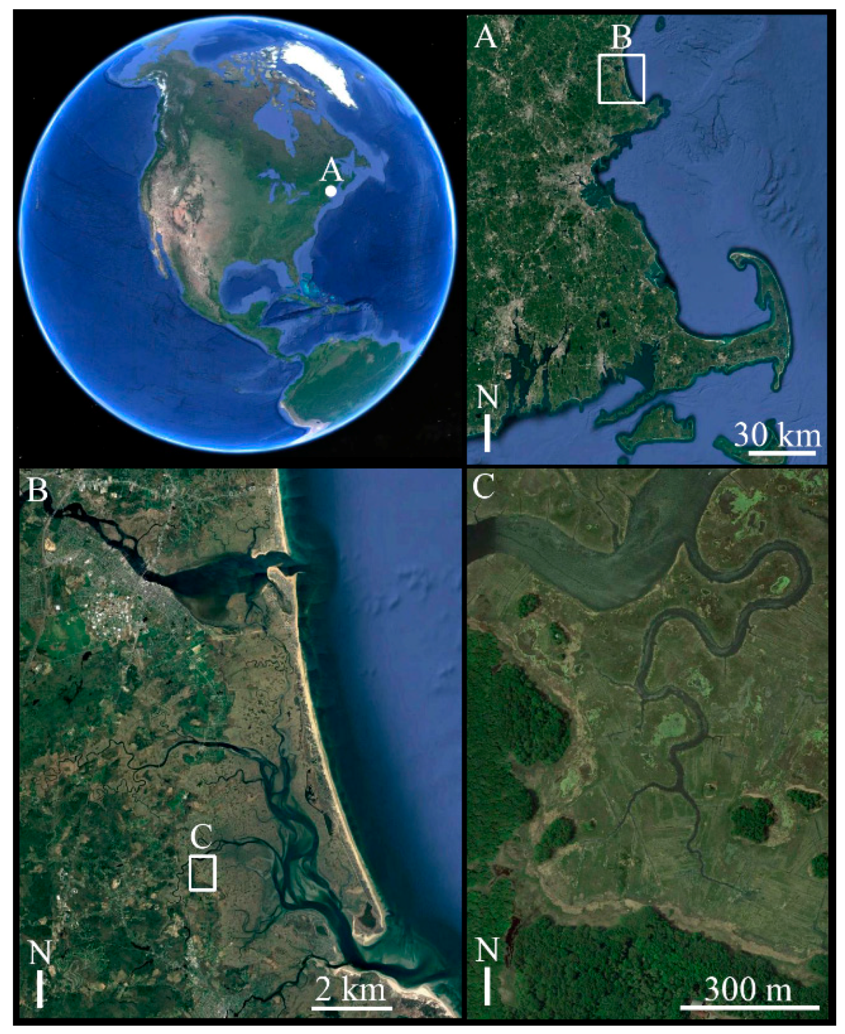
This multi-year study investigated how airborne light detection and ranging (lidar) observations can characterize saltmarsh ecosystems by providing detailed classifications, representations of vegetation and geomorphology, and snapshots of phenological state. From 2014 to 2016, airborne lidar observations of a saltmarsh in a National Science Foundation Long Term Ecological Research (LTER) site in Plum Island (Massachusetts, United States) were carried out by National Aeronautics and Space Administration (NASA) Goddard Lidar Hyperspectral and Thermal (G-LiHT) airborne instrument package (Figure 1). This study was intended as an extensive pathfinding effort to establish the strengths and limitations of airborne lidar in a well-studied saltmarsh, providing insight for planning future wider-scale survey efforts in mid latitude saltmarshes, and refining interpretations of satellite imagery time series. Although G-LiHT is a multi-instrument package, and includes a hyperspectral imager, the airborne lidar data were the focus of this study (noting that the illumination and aerosol conditions at the times of overflights were suboptimal for hyperspectral retrievals). The lidar observations from G-LiHT were supported by terrestrial lidar observations and spectroscopy measurements, conducted concurrently to G-LiHT overflights, and at key phenological stages throughout 2015 and 2016. Landsat 7 and Landsat 8 observations were also used to evaluate the potential of G-LiHT airborne lidar observations for characterizing saltmarshes.
Saltmarshes are grasslands associated with freshwater outflows to low-energy coastal systems, and are regularly inundated by salt or brackish water [1,2]. They are formed by accreted sediment, colonized and stabilized by a succession of algal species and halotolerant terrestrial grasses [3]. Saltmarshes are globally distributed, but mostly restricted to areas of temperate climate, and higher latitudes [4]. The strong gradients and fluctuations of salinity in saltmarshes, controlled by the interactions of tides and topography, result in conserved zonation of vegetation species [5,6,7].
The importance of saltmarshes to both blue carbon sequestration [8,9] and to coastal armoring [10,11] have been well established. Saltmarshes are some of the most productive coastal ecosystems in terms of carbon fixation [12] and, alongside the other blue carbon ecosystems of mangroves and seagrass beds, have been established as important sinks for carbon [8,13,14,15]. Furthermore, saltmarshes greatly contribute to coastal shoreline protection [10,16], reducing the physical impact of waves [11,17] on habitats and infrastructure inshore, thereby mitigating the potential socioeconomic impacts of storm events and sea-level rise [18,19].
Additionally, saltmarshes serve as filters for terrestrial nitrogen inputs to coastal systems, buffering nitrogen-loading of near-shore areas [20] and therefore limiting eutrophication events and harmful algal blooms [21]. Furthermore, saltmarshes provide habitat for commercially important aquatic species [22,23,24,25], and migratory birds [26,27,28], representing a high endemic biodiversity [29].
However, saltmarsh ecosystems, and their concomitant services, are subject to chronic and increasing pressures [30,31,32]. Potentially perturbing factors include nutrient enrichment [33,34,35], chemical contamination [36,37,38,39], radioactivity [40,41], sea-level rise [42,43] and coastal land-use changes [27,44,45,46]. Sea-level rise [18,47] and more frequent storm surge [19], both associated with global climate change, have a large impact on saltmarsh extent, hydrology and salinity. Changes in sea-level and extreme weather events directly cause erosion and sand deposition, reducing vegetation growth and overall saltmarsh extent [43,48]. Changes in salinity distributions are believed to be responsible for the prominent invasion of the common reed Phragmites australis, which is spreading rapidly and creating monocultures in temperate saltmarshes [49,50,51].
The potential long-term changes to saltmarsh extents, conditions, and services, together with the long history of active ecosystem management in saltmarshes [52], have encouraged interest in monitoring these ecosystems with remote sensing resources. The wide and frequent coverage, and the ever-expanding long-term record of satellite resources is particularly appealing for monitoring saltmarshes. For example, in combination Landsat 7 and Landsat 8 provide an eight day repeat coverage of most regions, while the more recently launched Sentinel-2a and Sentinel-2b, in combination, offer a five day global repeat coverage.
Despite increasing public access to moderate resolution satellite resources, it continues to be challenging to characterize saltmarshes with passive optical satellite resources alone. Observations of coastal ecosystems from satellites are frequently contaminated by persistent cloud cover [53,54], and New England saltmarshes such as Plum Island are periodically covered by ice and snow during winter. Saltmarsh vegetation species form spectrally distinct cover types, existing in adjoining, relatively pure patches, with horizontal extents typically on the order of meters, controlled by the hydrology, topography and geomorphology of a particular saltmarsh. This mosaic-like ecosystem composition means that typical satellite pixels with resolutions of tens of meters, will contain multiple cover types, and frequently multiple, separate patches of each type [55]. Furthermore, each satellite observation can include a highly variable amount of water of varying turbidity, depending on the specific footprint of the observation, the tidal state at the time of overpass, and sediment loading and run-off. Extreme inundation events such as storm surges that submerge upland areas of saltmarshes can restructure hydrology [19,56], and cause substantial changes in biology [57] over a short time-scale, further confounding satellite observations.
Airborne lidar instruments can overcome some of these challenges by providing the high spatial resolution of structural information required to distinguish between the different cover types found in saltmarshes, and mitigating the effects of variable atmospheric and soil moisture conditions with active measurement [58]. Previous studies have utilized both discrete and full-waveform airborne lidar to delineate various saltmarsh components, including vegetation types and species, by their relative heights [59,60,61,62]. The cover of invasive Spartina species has been successfully discriminated by height in airborne lidar observations of California saltmarshes [63]. Surface terrain models, and the depth of saltmarsh vegetation have also been derived [64,65,66,67], although airborne laser scanner data was found to struggle to penetrate dense saltmarsh vegetation [68] and overestimate heights in several vegetation types [69]. Airborne lidar have also been used to derive flow paths for hydrologic connectivity analysis [70]. Furthermore, an evaluation of the challenges of acquiring airborne lidar data suggested that flight times, and filtering and interpolation algorithms, required additional consideration in saltmarshes [71].
Synthesis of lidar with high resolution multispectral data has been recommended for saltmarsh studies, so that both structurally distinct and spectrally distinct components can be classified effectively [72,73]. Fusion of hyperspectral and lidar data has been used to improve habitat and vegetation classifications and quantification [68,74,75,76,77,78], and monitor carbon stocks [79]. The relative intensity data from dual-wavelength airborne lidar instruments has been utilized for characterization of vegetation and zonation [80]. Optical and lidar acquisitions have also been combined with Synthetic Aperture Radar (SAR) to offer classified models of vegetation that include vegetation height [81]. SAR has also been utilized to detect change in the extent and composition of saltmarshes [82,83,84]; measure topography [85]; monitor storm surge and flooding [86,87,88]; burn recovery [89]; hurricane recovery [90,91]; oil spill impacts [92,93,94,95]. Structure from motion has enabled digital imagery to provide equivalent structural representations to lidar, permitting the retrieval of leaf area index from Spartina alterniflora [96].
Although airborne lidar have proven useful in characterizing saltmarshes, alone and when synthesized with other instruments, acquisitions of airborne lidar for any given saltmarsh region are inevitably much less frequent than acquisitions of multispectral satellite data. Additionally, airborne lidar observations of saltmarshes are challenged by occlusion of topography by vegetation [97]; water and soil moisture absorption [98,99]; and complex geomorphology [100].
Therefore, the role of airborne lidar has to be in the provision of characterizations that refine the interpretation of satellite observations of saltmarshes. Airborne lidar can conceivably achieve this aim by providing estimates of baseline conditions to contextualize satellite observations of saltmarshes, as well as by mitigating uncertainties due to the particular sensitivities of satellite observations, such as to the complex arrangement of vegetation patches [55], and to the highly dynamic coverage of variation in water turbidity.
The maximum performance, variety and remaining limitations of airborne lidar applications for saltmarsh characterization and monitoring in a New England saltmarsh were investigated. The saltmarshes of the north-eastern, New England region of the United States are recognized to be of a conserved archetype, owing to their shared geological substrate and history [101,102]. This regional comparability of saltmarshes that belong to distinct watersheds and bays has long made the saltmarshes of New England an appealing subject of study, particularly since they have been subjected to a variety of anthropogenic impacts dating back to the 17th Century [103,104]. These anthropogenic impacts include extensive modification of hydrological features, such as the addition of ditches branching off from natural tidal creeks [103]. These ditches aimed to reduce standing water, and accelerate drainage of the marsh platform after inundation [105]. The true long-term effects are still under investigation. The general ecology [103,106], and particularly vegetation community structure, and its determining factors have been well-studied in the region [107,108,109,110,111].
NASA’s G-LiHT airborne instrument package was able to acquire observations in three consecutive years, in an area that is particularly well-studied within the Plum Island Estuary LTER. The study site is also that of the NSF-funded Trophic cascades and Interacting control processes in a Detritus-based aquatic Ecosystem (TIDE) project, which studied the influence of nitrate enrichment on physical, chemical and biological attributes of saltmarsh ecosystems. Focusing G-LiHT’s acquisitions on this area enabled the use of existing data from historical and ongoing studies, and provided the opportunity for acquiring additional complimentary ground acquisitions specifically for this study.
Classification maps, derived from G-LiHT airborne lidar, were evaluated for general vegetation, Spartina alterniflora, the invasive Phragmites australis, wrack (dead, detached vegetation), exposed soil, water, and algae. In addition, the ability of G-LiHT to capture creeks and ditches, pools and pannes, vegetation composition, and vegetation volume are assessed using coincident data. Terrestrial lidar acquisitions provided validation for some G-LiHT structural products, were used to produce pathfinders for hybrid models to refine satellite interpretations, and were used to form simulations to guide specifications for future airborne lidar data acquisitions in temperate saltmarshes.
2. Materials and Methods
2.1. Study Site
Plum Island is a sand-based barrier island [112] in New England (Massachusetts, United States), which fronts onto the Gulf of Maine (Figure 1). Shielded by Plum Island, the 25 km Plum Island Sound is the largest wetland estuary in New England. The Sound comprises, from the closed end in the north to the open end in the south, the watersheds of the Parker, Rowley and Ipswich Rivers. The central region of the Rowley River watershed is occupied by a typical New England saltmarsh [113]. Plum Island was declared a LTER site in the National Science Foundation’s (NSF) LTER network, in 1998. The specific region of interest for this study is: Northwest corner: 42°43′36.90″N, 70°51′11.27″W; Southeast corner: 42°43′6.34″N, 70°50′36.07″W. This is the site of the NSF-funded Trophic cascades and Interacting control processes in a Detritus-based aquatic Ecosystem (TIDE) project.
2.2. Airborne Lidar
Airborne lidar observations were provided by NASA G-LiHT [114]. The lidar instrument included in G-LiHT is the Riegl VQ-480, a 1550 nm laser scanner which produces discrete returns with onboard waveform processing. At the standard operating height of 335 m above ground, this airborne lidar achieves a ranging accuracy of 25 mm over a 60 degree swath, resulting in a ground swath 387 m wide (Figure 2). The beam divergence of 0.3 mrad results in a typical beam diameter of 10 cm on the ground. A preliminary G-LiHT acquisition of Plum Island was made in June of 2014, which was used to plan for a ground campaign to support another acquisition in June 2015. A third G-LiHT overflight to expand monitoring of Phragmites australis extent was conducted in June 2016. The mean density of pulses on the ground was estimated to be 16.9 pulses/m2 (σ = 6.2) in 2014, 14.1 pulses/m2 (σ = 5.9) in 2015, and 15.3 pulses/m2 (σ = 6.0) in 2016. G-LiHT data are available from https://G-LiHTdata.gsfc.nasa.gov/.
Georeferencing of lidar data was achieved with information from an onboard INS/GNSS unit. G-LiHT lidar acquisitions are provided in georeferenced, LAS format. The co-alignment between acquisitions was manually adjusted based on common features. For the 2014 dataset, returns corresponding to a vertical misalignment of adjacent flight-lines, consisting of the minimum 3 m of height present in the dataset, was manually removed. For the 2016 dataset, returns corresponding to a horizontal misalignment of adjacent flight-lines were removed by filtering the relevant region by the angle of the pulses within the swaths.
2.3. Classification of Saltmarsh Components with Airborne Lidar
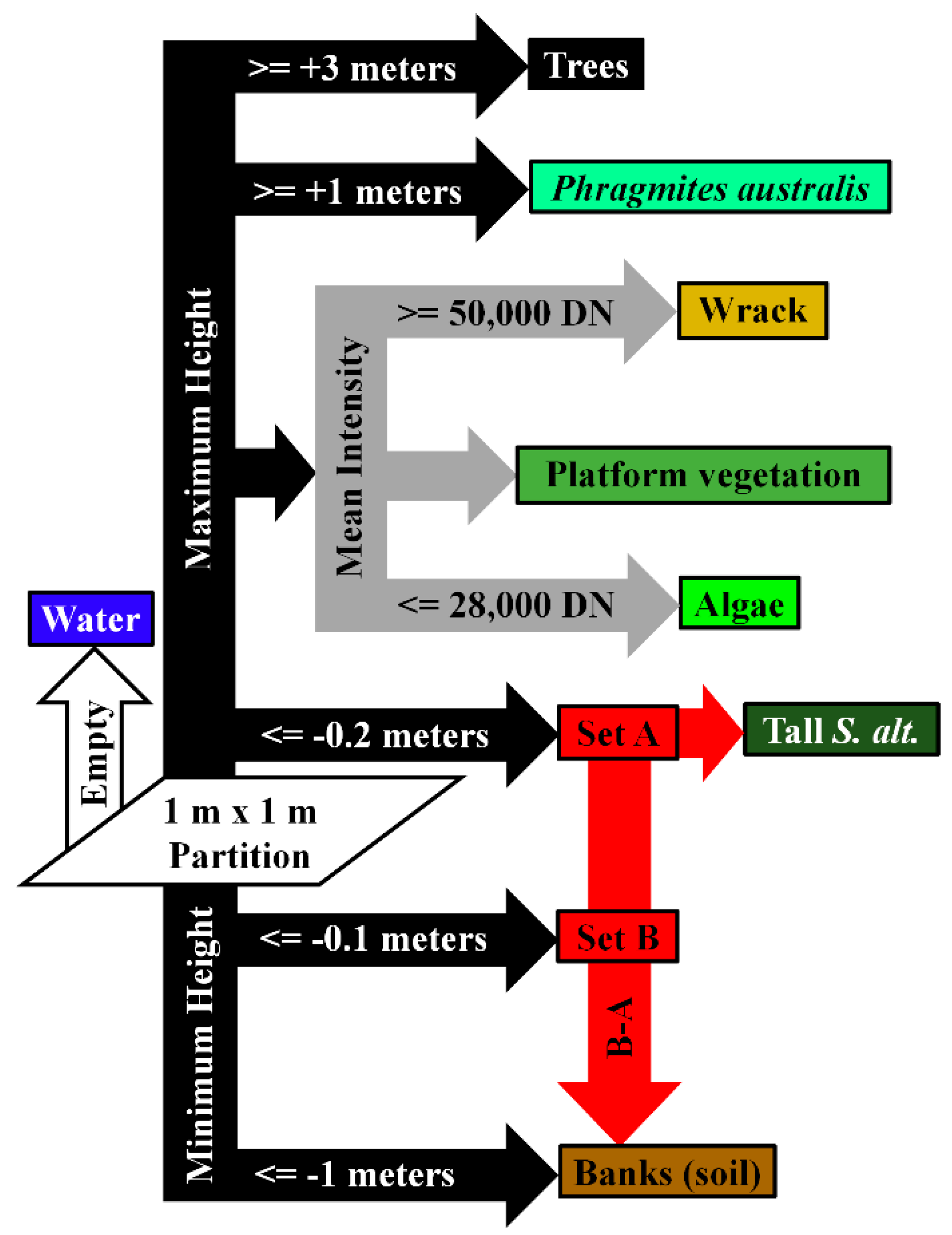
The classification of saltmarsh components was based on procedural assessment of structure, primarily as a function of height, and secondarily as a function of the intensity of recorded returns (Figure 3). Classifications were carried out across the study region for the 2015 airborne lidar acquisition. First, a grid comprised of 1 m-sided partitions was established over the data, and the maximum and minimum heights of returns were retrieved for each grid square. Height was interpreted relative to a datum of marsh platform height, derived from the mean height of returns occurring in the most-occupied 0.05 m height bin. Thresholds in height were determined with reference to terrestrial lidar and field observations. Thresholds in lidar intensity, used to separate components of the marsh platform, were determined with reference to terrestrial lidar data and airborne imagery.
The first stage of the classification procedure utilized thresholds applied to the minimum and maximum heights of returns in each partition. This initial height-based assessment resulted in each partition either being directly assigned a classification, or being subjected to a further assessment based on the mean intensity of returns, or being included in a set and subjected to set operations (Figure 3). Height thresholds were determined with reference to the terrestrial lidar and field observations acquired during this study. Partitions containing no returns were given a classification of water. The relative complement of the sets from the central range of heights were classified as exposed soil of creek and ditch banks, while the remainder (functionally, the intersection of the two sets, plus the inverse of the previous relative complement) were classified as tall Spartina alterniflora (Figure 3). Thresholds in the mean intensity of the 1550 nm lidar returns were used to reclassify some of the marsh platform grid squares as wrack (DN ≥ 50,000), or algae (DN ≤ 28,000).
2.4. Terrestrial Lidar
Terrestrial lidar observations were acquired with University of Massachusetts Boston’s Compact Biomass Lidar (CBL), an instrument optimized for rapid acquisition in the short time windows permitted by the tidal cycles of saltmarshes, and compatible with special deployment platforms optimized for acquisitions in saltmarshes [115]. The CBL is a 905 nm instrument with ranging error of ±30 mm.
Acquisitions to monitor Phragmites australis extent and growth, to characterize marsh platform pannes, and derive vegetation maps for comparison to G-LiHT lidar, were conducted throughout 2015 with the CBL mounted on a tripod, with an optical center height of 1.3 m. Acquisitions for representing the specific geomorphology of sections of creek were conducted during April 2015, while vegetation was absent, and with the CBL mounted on a tower deployment system [115]. All co-location of terrestrial lidar data was achieved with an initial automatic co-location based on measured field location, followed by manual adjustment by an experienced operator, based on observation of common features, including targets placed while in the field.
2.5. Volume and Surface Area Estimates from Lidar
Volumes were estimated for vegetation and water components from airborne and terrestrial lidar data. The method utilized is described as square-based column projection in [116], and is simply the sum of volumes of cuboids of regular cross-sectional area, arranged in a grid, and of height equal to the distance to lidar points encountered relative to an established reference plane, or reference surface. For vegetation volume, the reference plane was the marsh platform, and the distance to lidar returns estimated the height of vegetation in each cuboid. For water volume from tidal models, the reference surface was the structure of the creek bank observed with terrestrial lidar. A reference plane was added to span the bottom of the creek, since even at the lowest tidal level during observations, some creek structure was obscured from lidar observations by water that absorbed the lidar energy. The visible surface area of water for a given tidal height was derived by summing the area of grid-squares in which the height of the tide relative to the reference plane exceeded the height of the creek bank reference surface.
2.6. Ground Spectroscopy
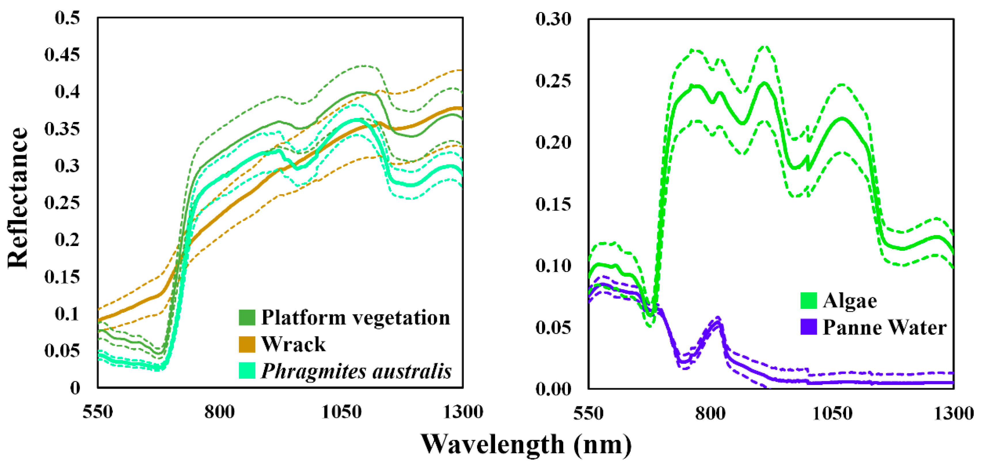
For several applications in situ spectroscopy measurements were also used. Plant and leaf level spectroscopy have previously been used to study saltmarsh components and their relationship to satellite observations [117,118]. These were acquired with an ASD FieldSpec spectrometer on 28 August 2015 (Figure 4), simultaneous to a Landsat 8 overpass. The weather conditions were predominantly clear with scattered clouds. Measurements were made only when clouds were not obscuring, or close to obscuring, the sun. Measurements were made with an eight degree field-of-view, and a Lambertian white panel was utilized for calibration prior to each measurement. For the spectral signatures used in linear combinations, between four and twenty ASD measurements were made of different patches of each saltmarsh component. These were assessed to potentially discount contaminated observations, although none were found among the observations. As end-members for linear combinations, the mean of the integrated reflectance within the relevant spectral bands of Landsat 7 and Landsat 8 was used, convolved by the Relative Spectral Reflectance (RSR) (average of the reflectance at wavelength extents of the full width at half maximum values).
2.7. Airborne Imagery
High resolution aerial imagery were accessed through Google Earth and utilized for further comparisons and evaluations of retrievals.
2.8. Tidal Height
Where estimates of tidal heights were required for analyses, the National Oceanic and Atmospheric Administration (NOAA) Center for Operational Oceanographic Products (CO-OP) six minute interval predictions were utilized. The Station ID for tidal predictions was 8441241 (Plum Island South, south end). Tide heights from this source are relative to the datum of mean lower low water.
2.9. Airborne and Terrestrial Lidar Hybrid Model
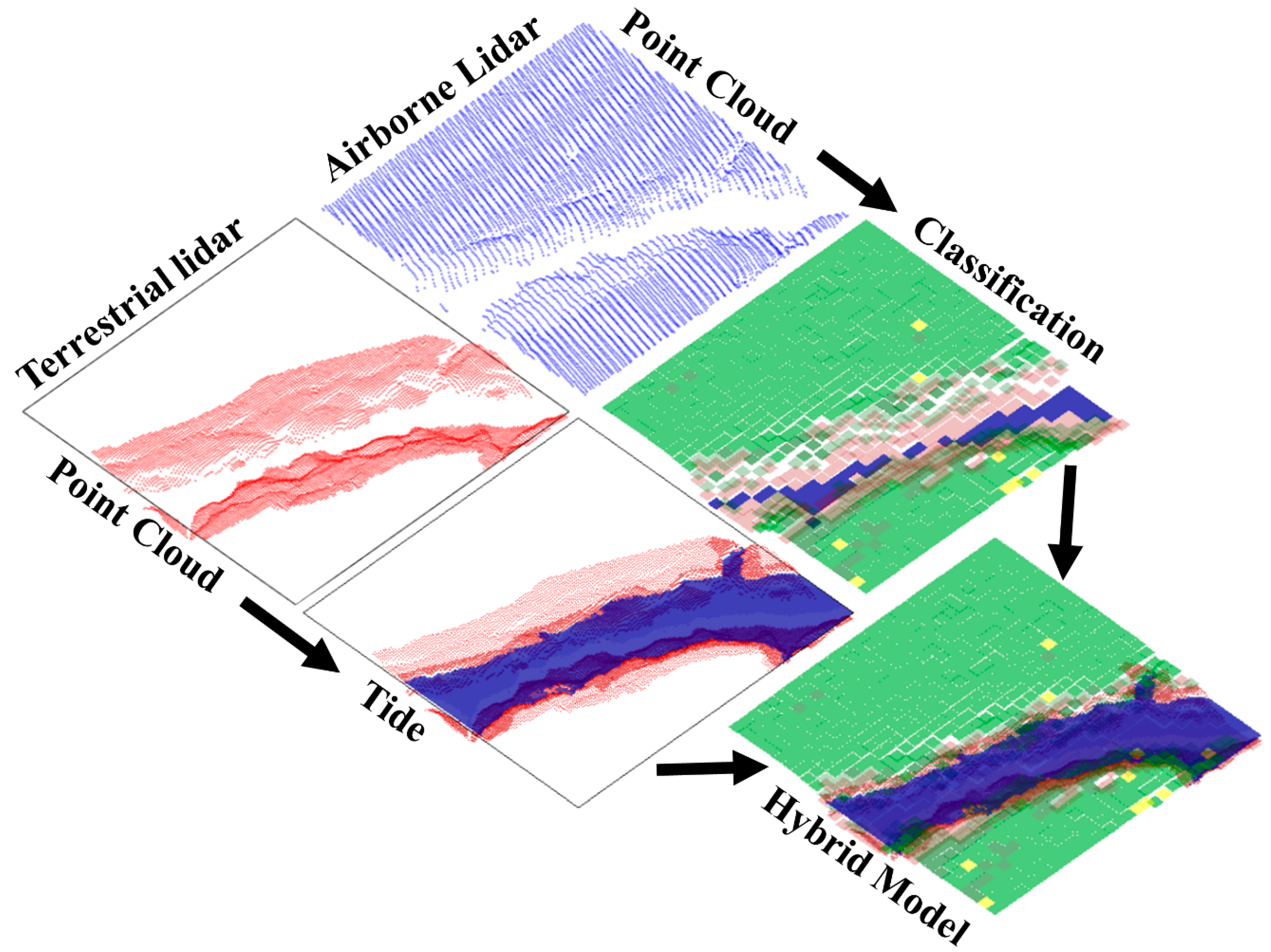
To address the influence of the discrepancy in tidal height, and therefore water coverage, between the time and date of the airborne classification model (1.9 m, 10 June 2015) and the Landsat 8 overpass (2.71 m, 8 August 2015), water coverage was modelled via the synthesis of airborne and terrestrial lidar data (Figure 5). A Landsat pixel prominently featuring a tidally active creek was identified, and a detailed representation of the geomorphology of the creek within the pixel was acquired with terrestrial lidar during April 2015, when vegetation was absent. An artificial water surface at the appropriate tidal height was added to the detailed geomorphological model (0.2 m resolution) to retrieve a refined estimate of water cover at the time of Landsat overpass. This tidal coverage model was then combined with the airborne lidar classifications of cover for the Landsat pixel, and linear combination with ground spectroscopy measurements for the various components were used to estimate Landsat 8 surface reflectance in the green, red and NIR (bands 3, 4, 5) [119,120].
2.10. Assessment of Hydrological Features
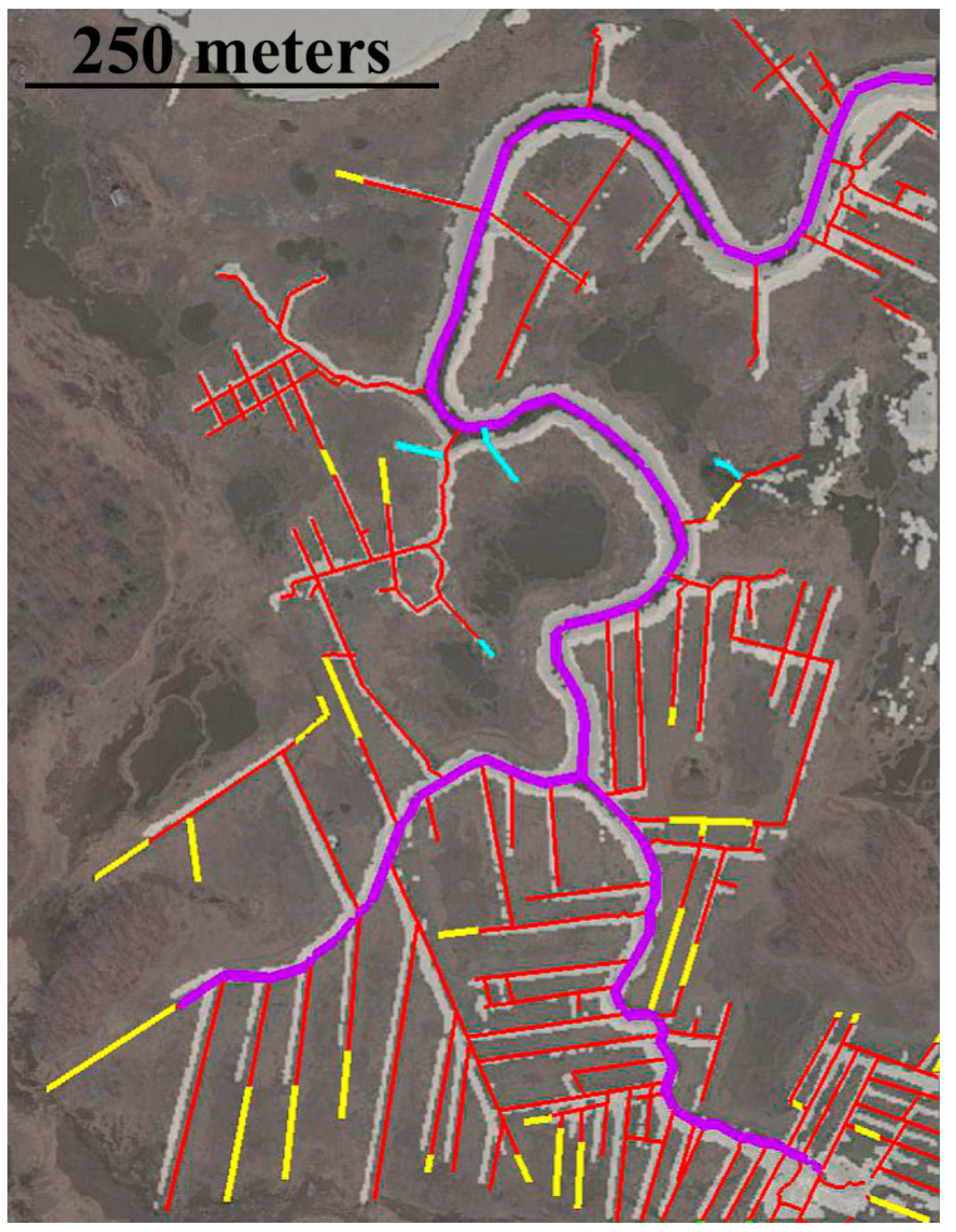
To evaluate airborne lidar retrievals of the tidally active hydrological features in the saltmarsh (creeks and ditches) the union of components in the 2015 airborne lidar classification that were found below the height of the marsh platform (water, exposed banks, and tall-form Spartina alterniflora) were compared to aerial imagery (Figure 6). Areas classified as water that were not within 5 m of either exposed banks or tall-form Spartina alterniflora was assumed to be in marsh platform pannes, and removed. To provide a quantitative assessment, vector maps were produced from high resolution aerial images from September 2014, June 2015, May 2016, April 2017 and April 2018. To maximize the completeness of the assessment map, creeks and ditches were traced independently for each airborne image, and separately by two operators, and the union of all of the representations was treated as the reference for creeks and ditches.
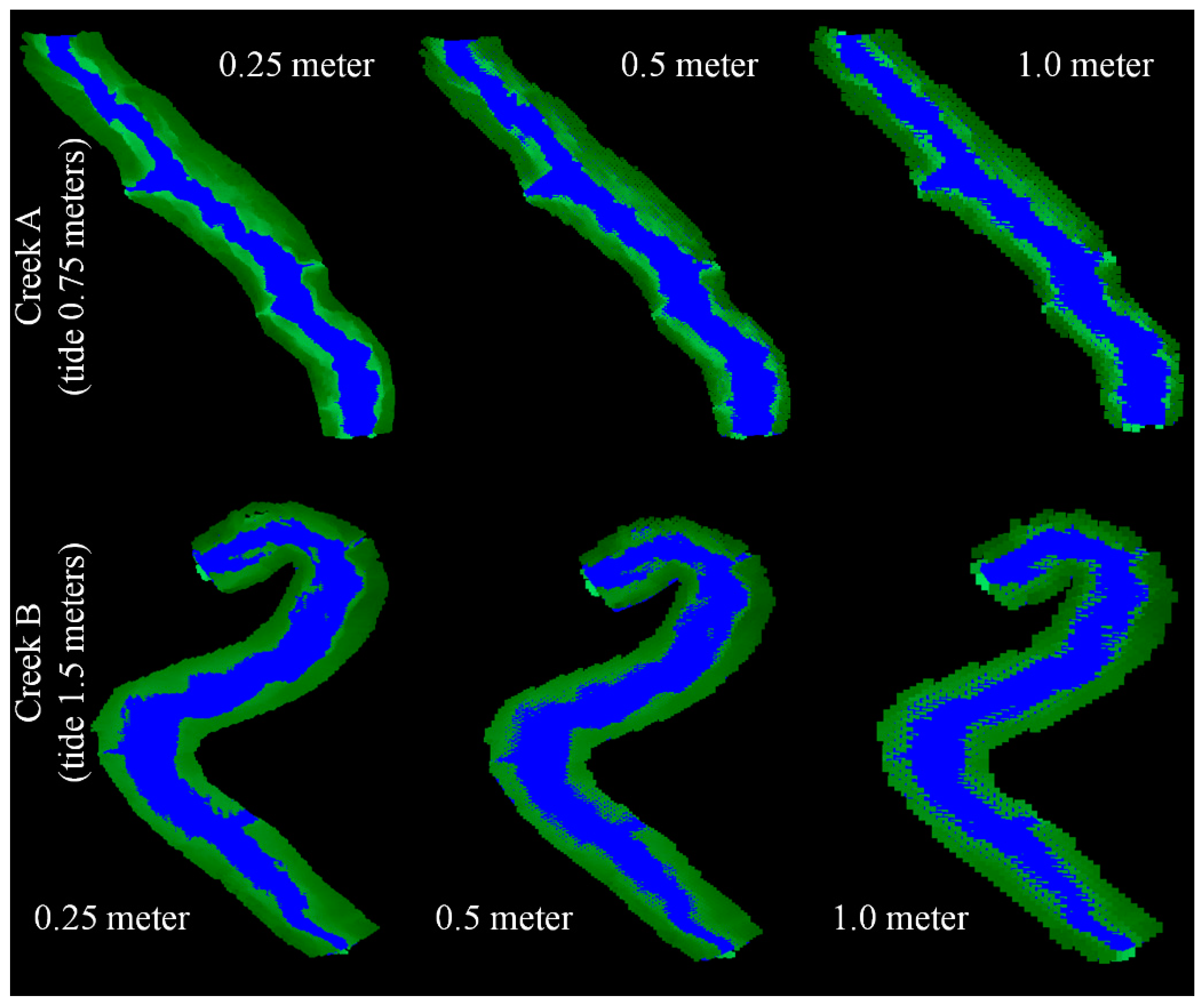
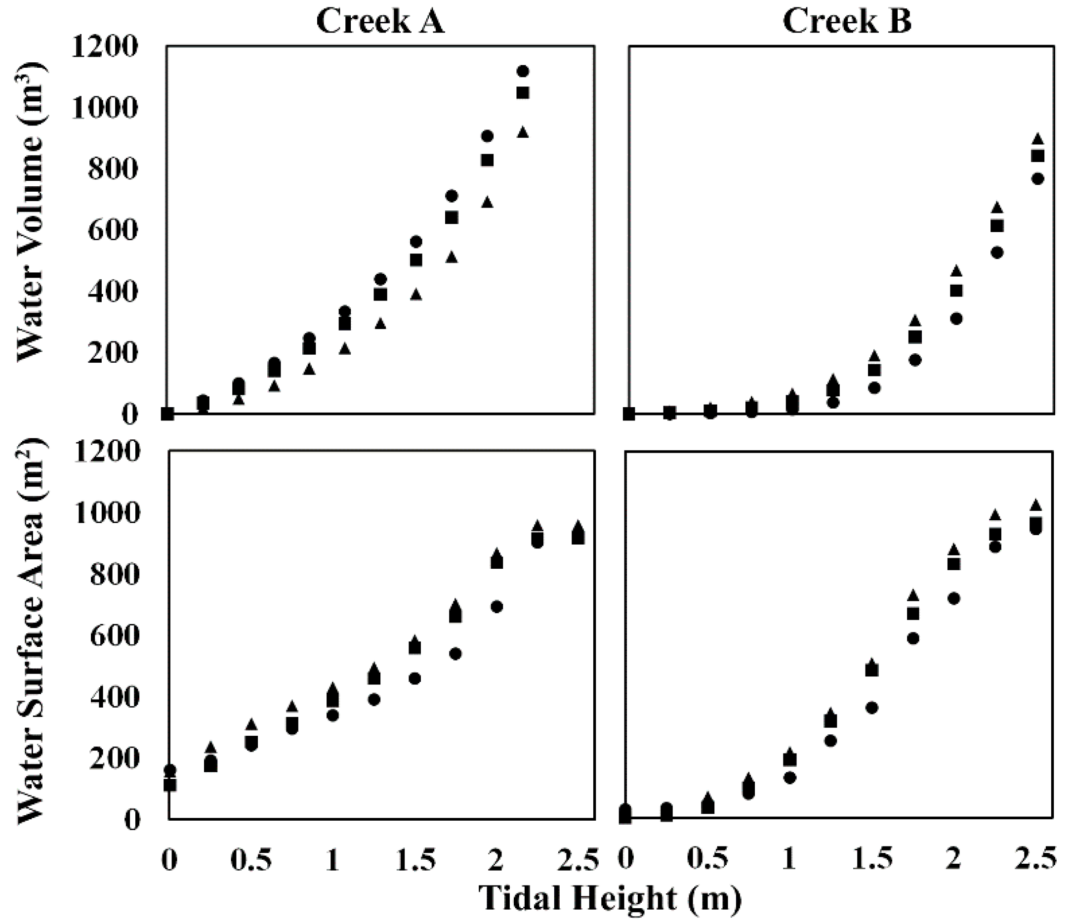
To investigate whether airborne lidar could make meaningful retrievals of geomorphology for saltmarsh tidal modelling, terrestrial lidar data was down-sampled, retaining the mean height of returns in each partition of grids arranged across the X and Y planes. 0.25 m, 0.5 m, and 1 m resolution representations of geomorphology were produced for two sections of saltmarsh creeks at Plum Island. Over a tidal height range of 2.5 m, estimates of water surface area and volume were retrieved for every 0.25 m increment of tidal height using the method described above (Figure 7).
3. Results
3.1. Classification and Representation of Saltmarsh Components
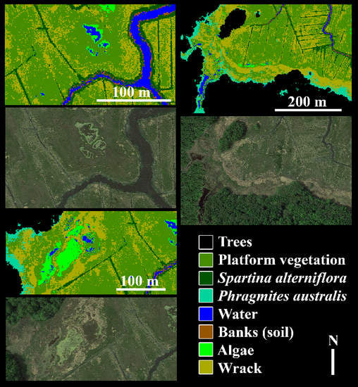
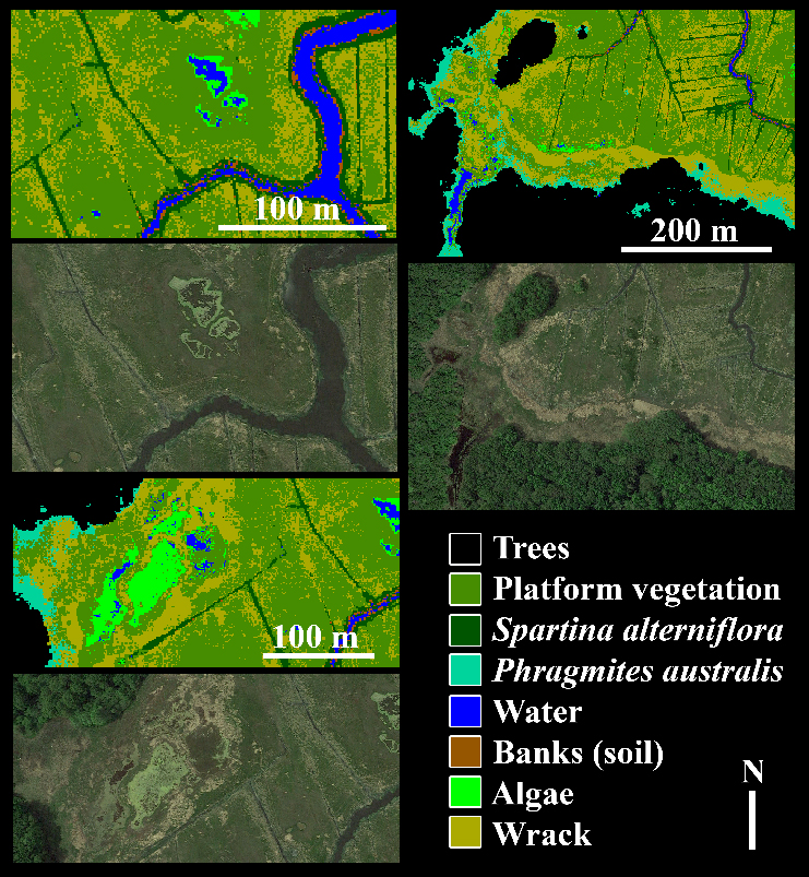
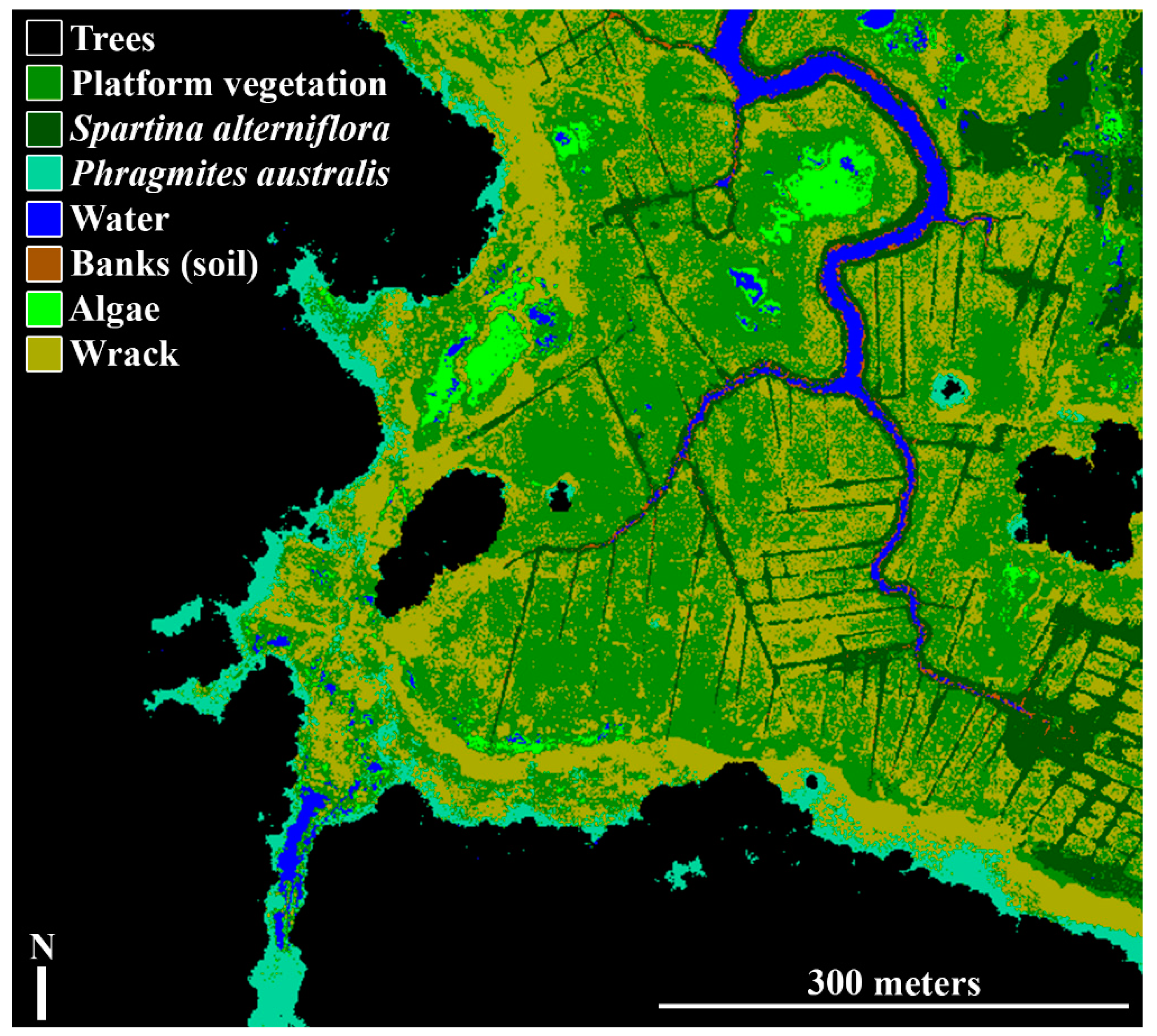
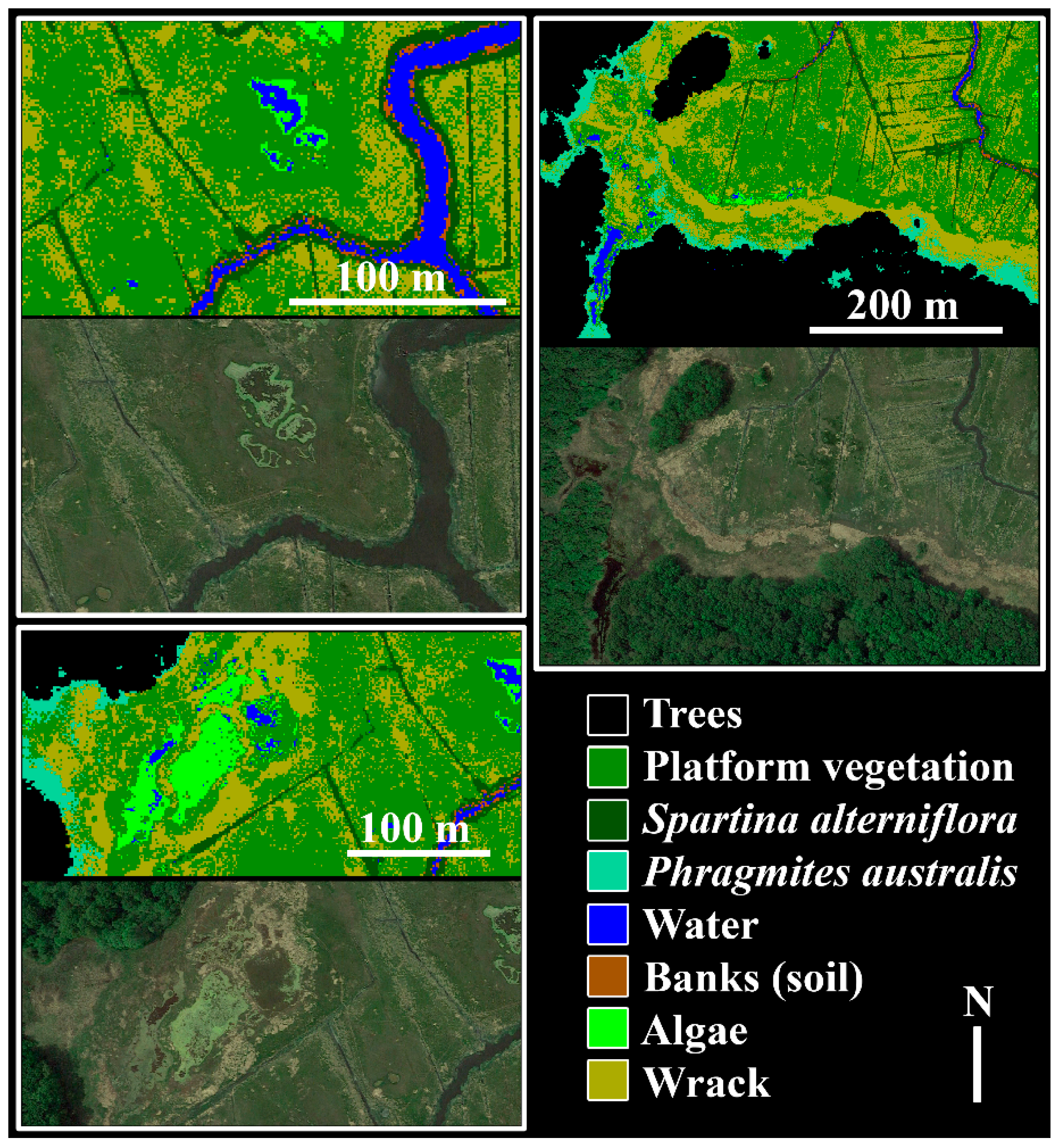
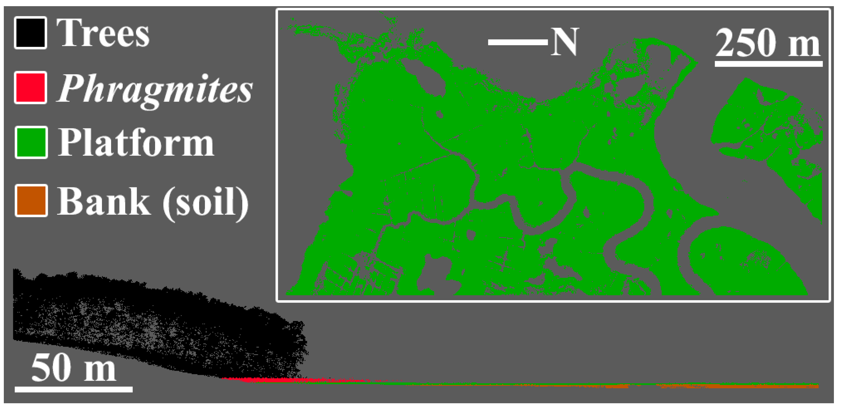
A 1 m resolution classification map was derived from the airborne lidar observations acquired in 2015. Aerial imagery was available from within three days of the G-LiHT overflight for evaluation. The initial impression of the airborne lidar classification of saltmarsh components is encouraging, with a plausible representation of the layout of the saltmarsh, and good agreement with high resolution imagery (Figure 8 and Figure 9). Vegetation types were all represented in the model in regions which jibe with their ecological niches and tolerances. Phragmites australis (total area: 16,958 m2) is constrained to the upland edge of the marsh, while tall form Spartina alterniflora (total area: 53,911 m2) has a strong spatial association with creeks and ditches.
The components of wrack (total area: 93,061 m2) and algae (total area: 7962 m2), delineated by intensity of the lidar returns, rather than estimated height, are well-represented in the 2015 dataset in qualitative comparisons to aerial imagery. The difference in tidal state between the airborne lidar classification and the aerial images is clearly visible in the difference in the areas of water (total area: 10,669 m2) in the creeks, and the increased visibility of the exposed soil of the creek banks (total area: 2339 m2). The remaining area of the lidar classification comprised general marsh platform vegetation (total area: 119,004 m2) and trees (total area: 221,992 m2).
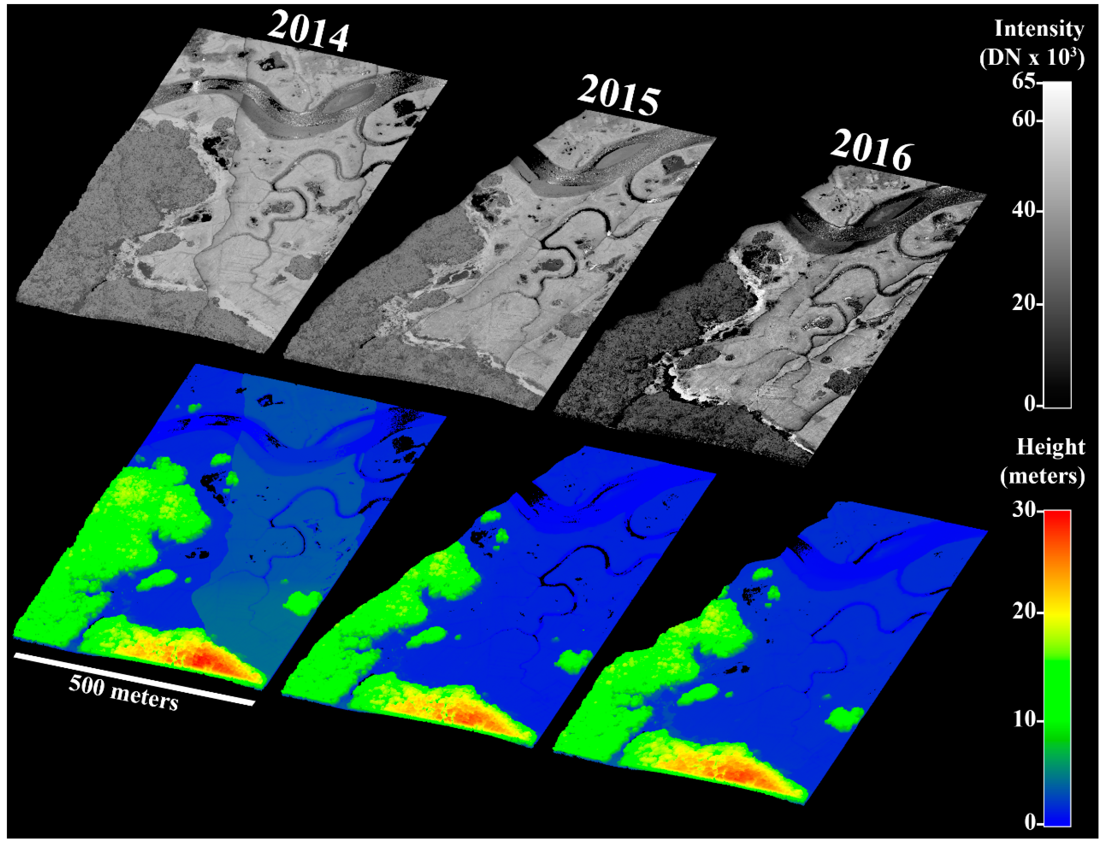
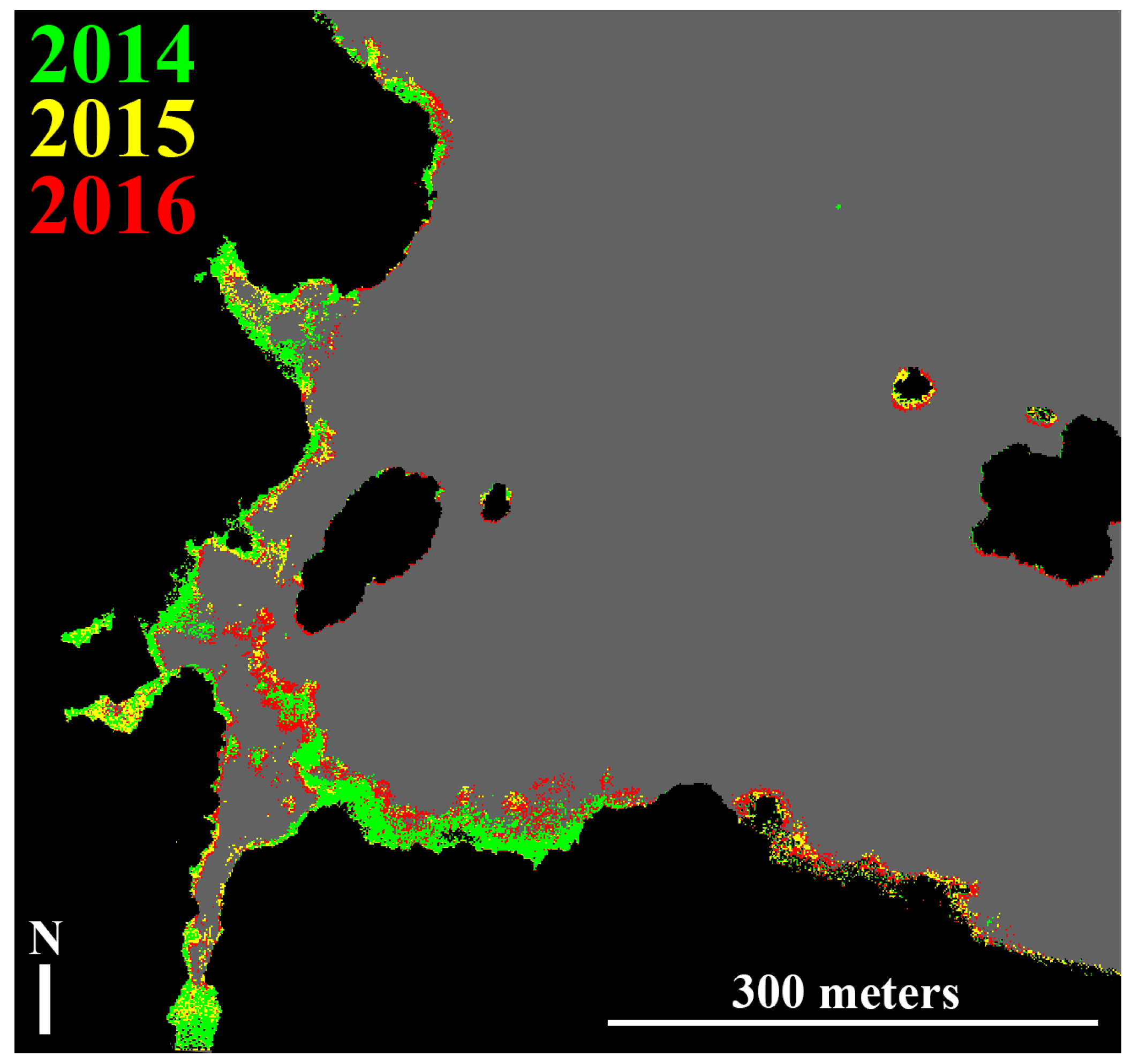
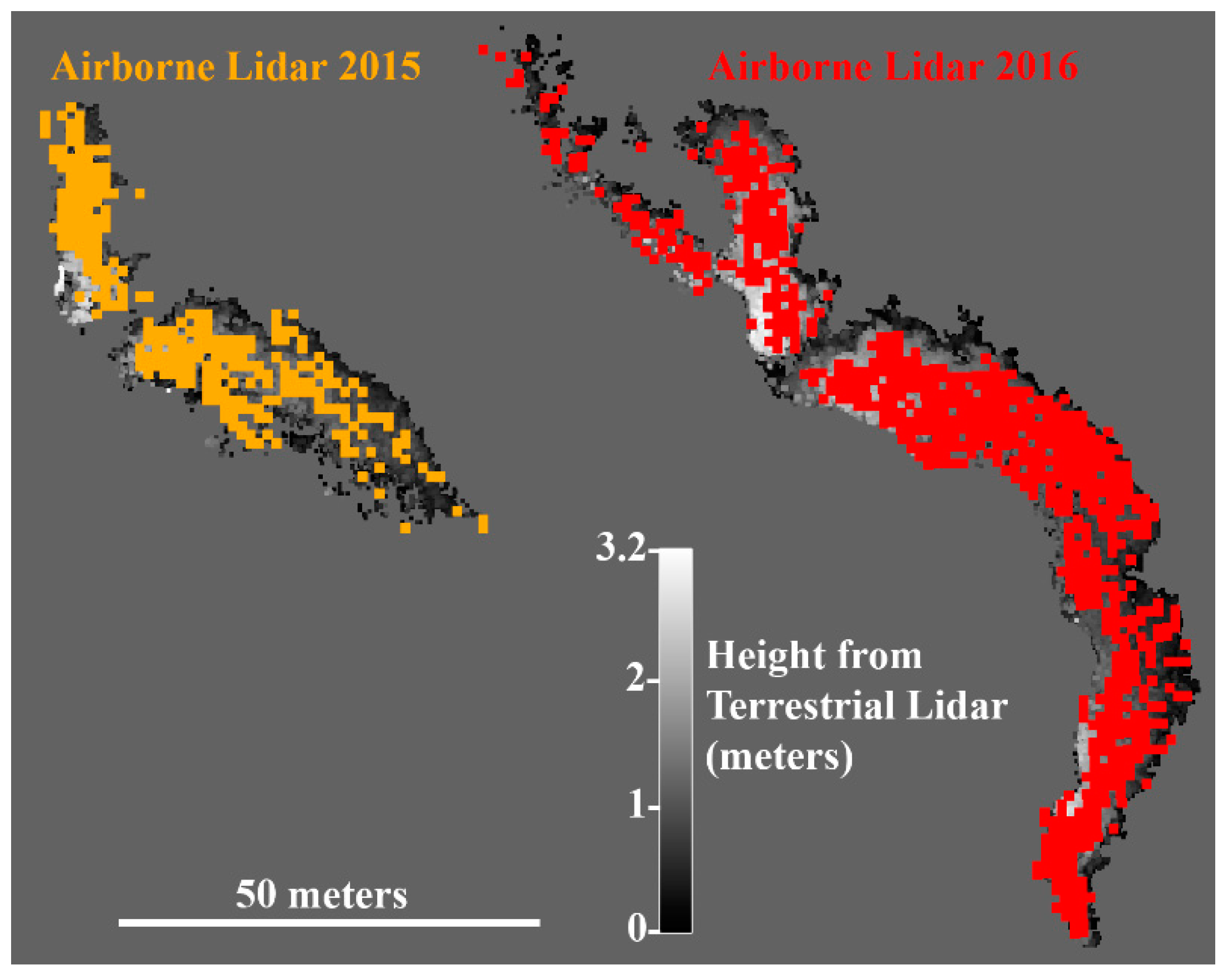
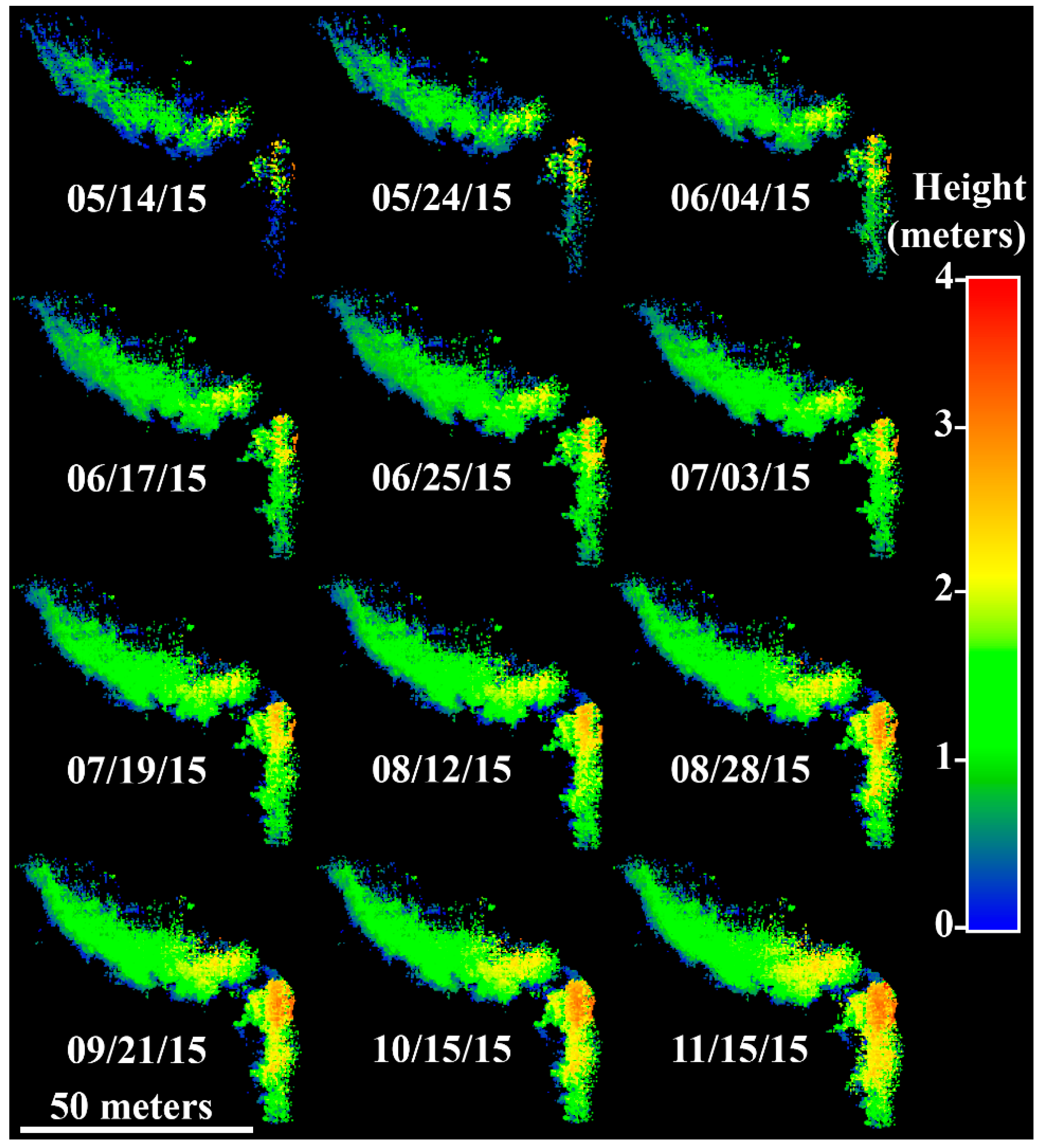
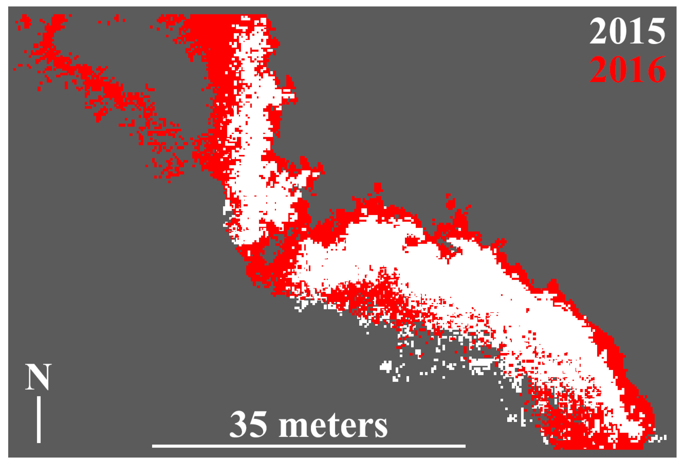
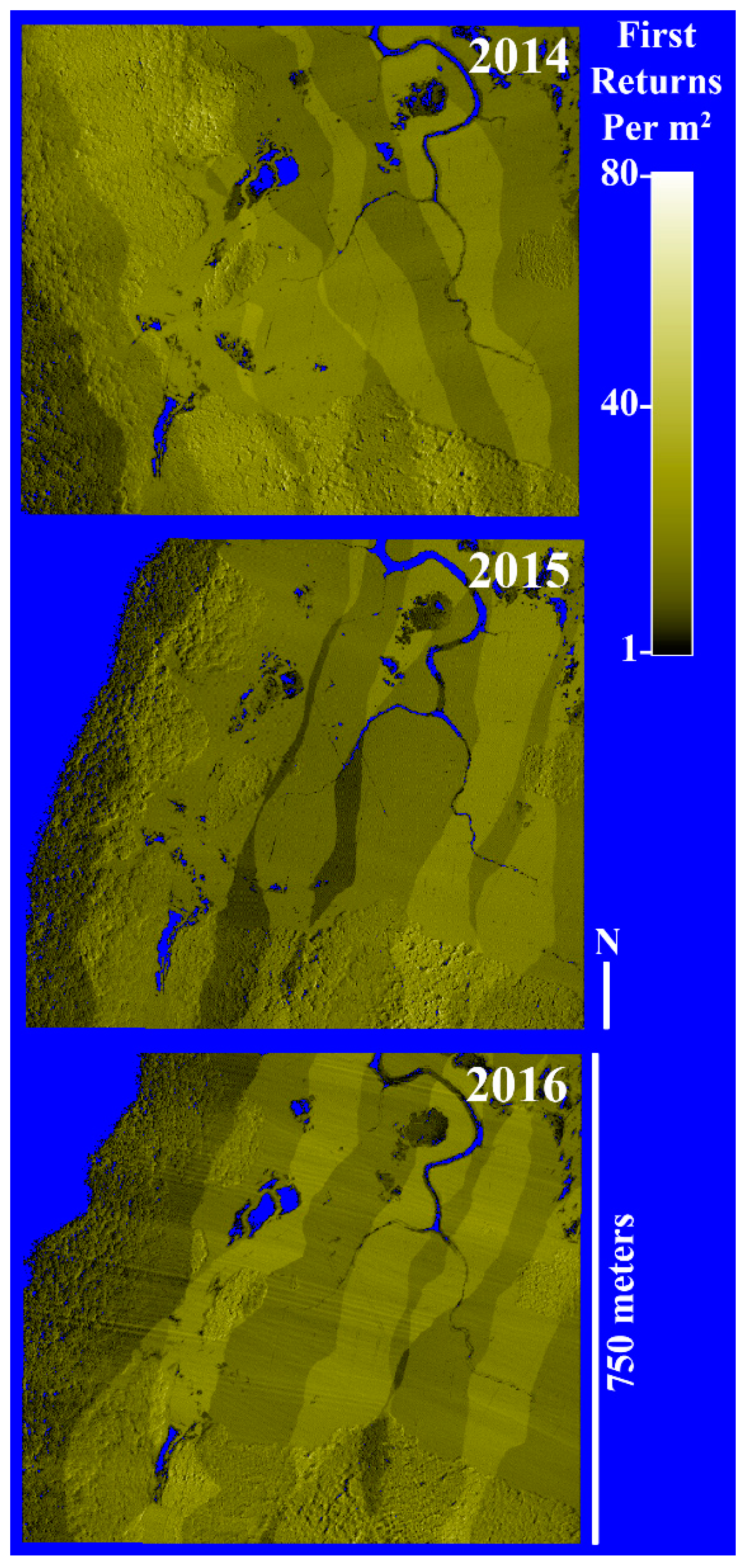
Subsequently, airborne lidar estimates of Phragmites australis cover were extracted for 2014, 2015, and 2016 (Figure 10). Phragmites australis cover increased from 8374 m2 in 2014, to 8882 m2 in 2015 (+6.1%), and again to 13,819 m2 in 2016 (+55.6%). Independent estimates for smaller areas derived from terrestrial lidar suggested the airborne lidar was underestimating Phragmites australis cover (Figure 11). In 2015, 438.7 m2 of Phragmites australis was found with terrestrial lidar, and only 281 m2 was found with airborne lidar in the same area (−35.9%). In 2016, an expanded terrestrial lidar survey found 1113.3 m2 of Phragmites australis in an area where the airborne lidar found only 763 m2 (−31.5%). The growth of a patch of Phragmites australis was also monitored with terrestrial lidar throughout 2015 (Figure 12, Table A1) with an estimated total gain in extent of 1317 m2, and an estimated total gain in volume of 676.3 m3 (±39.51 m3 based on ranging error) between 5th April 2015 and 11th November 2015.
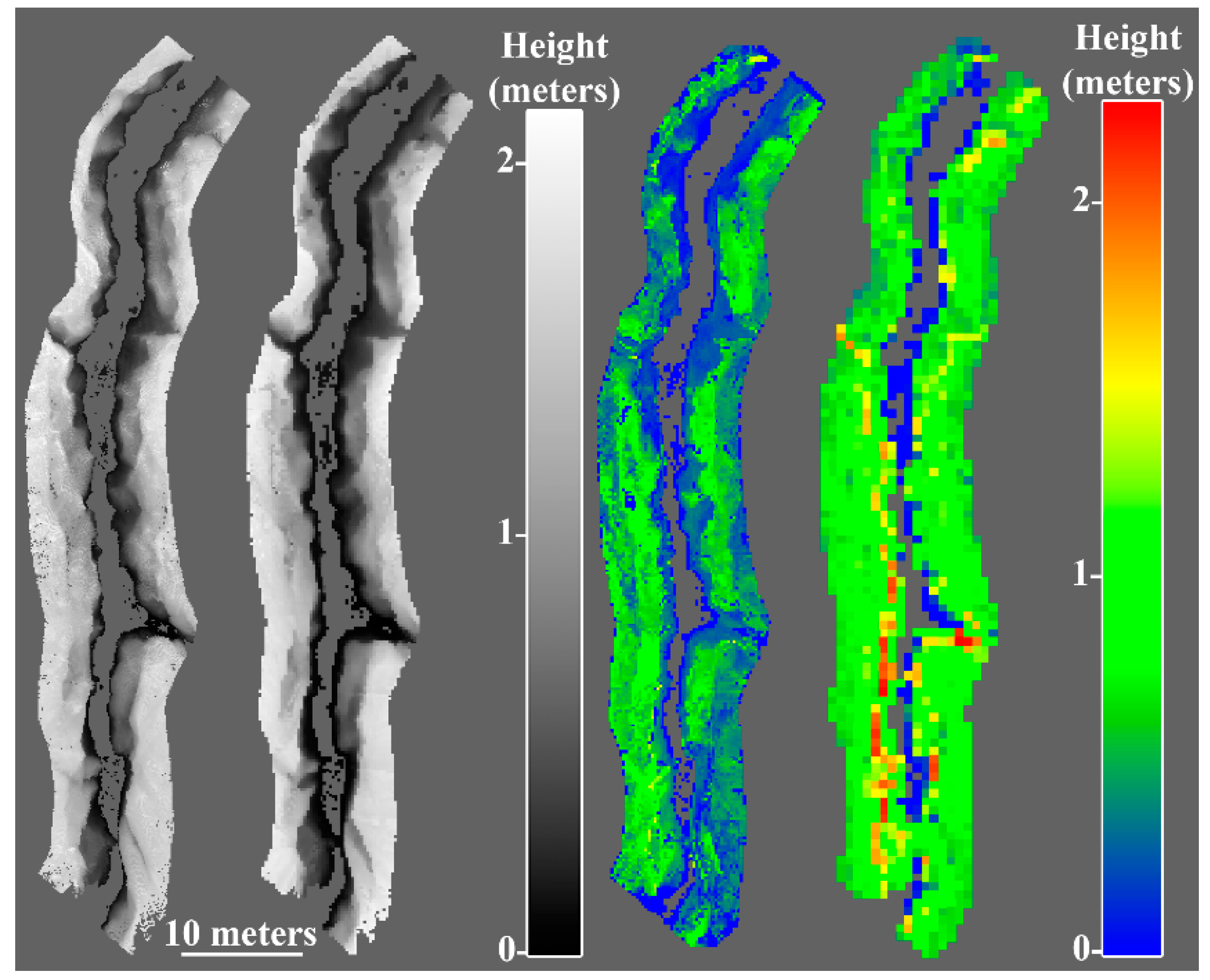
Terrestrial lidar observations of creek bank geomorphology, acquired during April 2015 while vegetation was dormant were used as a baseline surface for estimates of volume of tall-form Spartina alterniflora from both terrestrial and airborne lidar (Figure 13). Vegetation heights from 2015 airborne lidar (0.75 m resolution) produced a Spartina alterniflora volume estimate of 693.3 m3 (±21.6 m3 based on ranging error), which was 83.9% higher than that derived from terrestrial lidar vegetation heights (0.25 m resolution) acquired simultaneously (373.2 m3, ±23.98 m3 based on ranging error).
To evaluate airborne lidar retrievals of the creeks and ditches, relevant components from the 2015 classification were compared to aerial imagery (Figure 6). When assessing which sections of creek and ditch were represented in the airborne lidar classification, discontinuous sections were only counted as present if the section of creek or ditch airborne lidar also appeared discontinuously in both of the aerial images closest to the overpass in time (May 2016 and April 2017). Out of a total of 9084.3 m of creeks and ditches found in the airborne imagery, 8206.27 m (90.33%) were present in the airborne lidar classification.
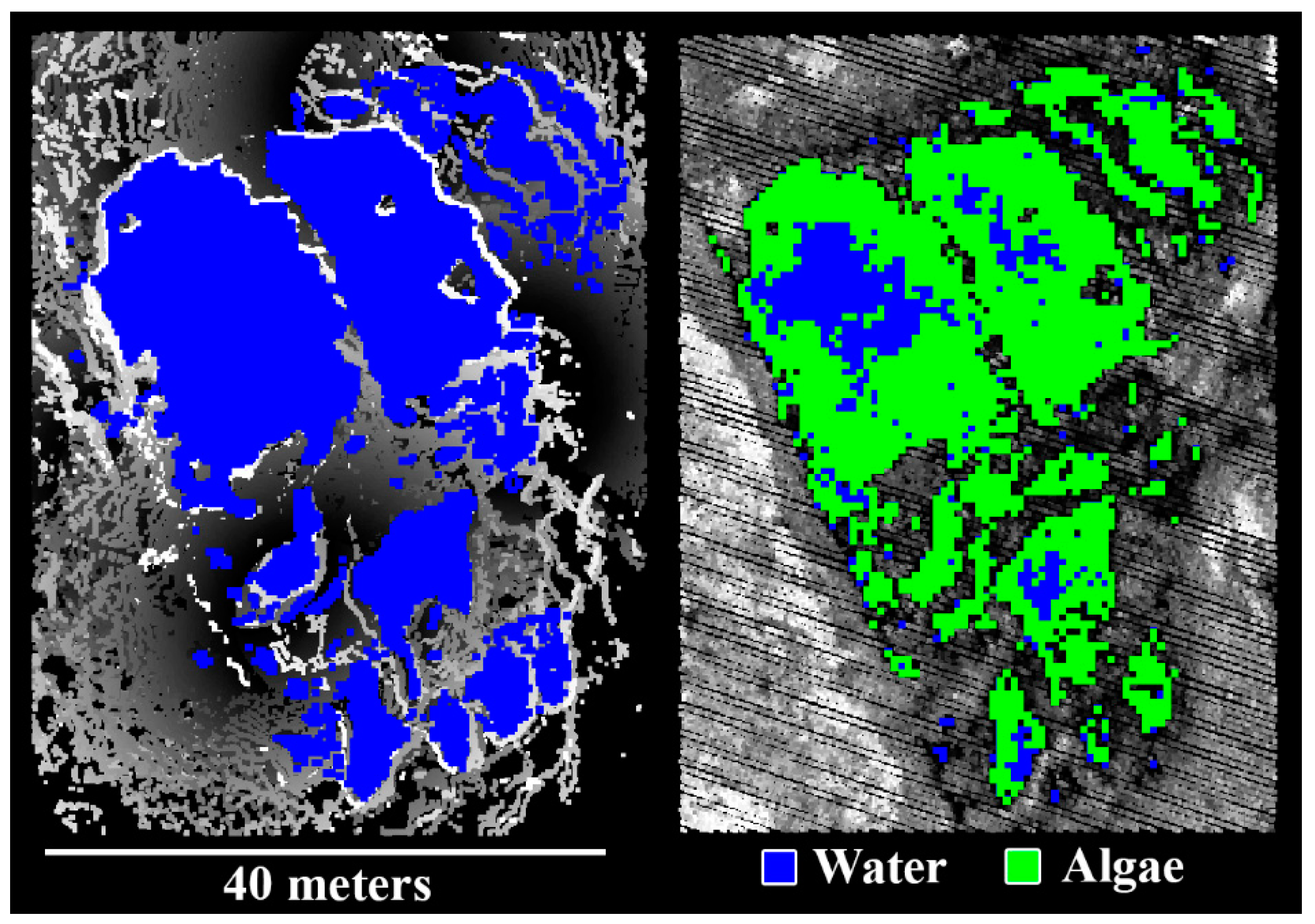
Detailed terrestrial lidar acquisitions of several adjacent pannes on the marsh platform were acquired simultaneously to the 2015 airborne lidar acquisition, and were used to derive estimates of area of standing water and algae to compare to airborne lidar estimates (Figure 14). Terrestrial lidar observations did not successfully capture surface algae, but produced a water cover estimate of 690.5 m2 (0.25 m resolution). The airborne lidar estimate of water coverage (0.5 m resolution) was similar to the terrestrial lidar estimate (768 m2, +11.2%), and was additionally able to estimate that algae covered 81.6% (626.5 m2) of the standing water.
3.2. Comparison to Landsat
For a Landsat pixel prominently featuring a tidal creek, a refined estimate of water coverage at the time of Landsat overpass was retrieved from a terrestrial lidar representation of the creek geomorphology, and combined with the airborne lidar classification and ground spectroscopy to refine predicted simulations of Landsat reflectance. The use of the airborne lidar classification alone produced reasonable predictions of Landsat reflectance for this pixel (green +18.88% error, red +18.4% error, NIR −3.50% error). However, estimations of Landsat reflectance were improved for all bands when derived from the airborne and terrestrial lidar hybrid model (green +9.29%, error, red +4.2% error, NIR −0.12% error) (Figure 5).
3.3. Simulation of Airborne Geomorphology Retrievals
Estimates of water volume and surface area from down-sampled terrestrial lidar data increased as tidal height increased for both creek samples, at all resolutions (0.25 m, 0.5 m and 1 m, Figure 7 and Figure 15). Estimates of volume decreased as the resolution of the terrestrial lidar representations of the geomorphology decreased (Table A2, Table A3, Table A4 and Table A5). Although the absolute disagreement between estimates of water volume at different resolutions increased with tidal height, the proportional disagreement decreased. For estimates of water surface area, estimates typically increased as the resolution of the terrestrial lidar representations of the geomorphology decreased, although there were exceptions at low tidal heights (Table A2, Table A3, Table A4 and Table A5). The absolute disagreement between estimates of water volume at different resolutions varied across the range of modelled tidal heights, though the proportional disagreement decreased.
4. Discussion
4.1. Airborne Lidar Characterization of Saltmarsh Features
Both qualitative comparison to aerial imagery and limited quantitative comparisons to terrestrial lidar and aerial imagery suggest the airborne lidar-derived saltmarsh classification model alone has potential. Examining the distribution of heights in the airborne lidar data, it is unsurprising that a model based primarily on delineation by height should be successful, given that the height ranges occupied by each of the classified components are extremely conserved (Figure 16). The marsh platform, for example, occupies only a 0.4 m height range across most of its extent. Utilizing structural information from airborne lidar data as a primary means of delineating saltmarsh components seems promising, at least for the type of saltmarsh found in the New England region.
Some components appear to be particularly well-characterized by the airborne lidar classification. One well-characterized component is the invasive reed Phragmites australis, which was a priority for characterization due to its formation of monocultures, and documented increase in many saltmarshes [49,50,51]. There was strong suggestion that Phragmites australis expanded both in existing regions, and into new regions between 2014 and 2016 (Figure 10). The airborne lidar-derived estimated area of Phragmites australis for the full region increased from 8374 m2 in 2014, to 8882 m2 in 2015, and again to 13,819 m2 in 2016. This observed rapid expansion between 2015 and 2016 is backed up by comparison to the terrestrial lidar estimates for the overlapping region (Figure 17) acquired in 2015 (438.7 m2) and 2016 (714.6 m2). However, the terrestrial lidar observations suggested that the airborne lidar may still be underestimating Phragmites australis cover (−35.9% in 2015, −31.5% in 2016).
The underestimation of Phragmites australis extent seems to correspond to a tendency of the airborne lidar classification to fail to capture Phragmites australis at the edges of the major patches shown in the terrestrial lidar classification. There are several possible reasons for this tendency. The Phragmites australis at the edges of the patches tend to be shorter individuals that might not meet the height thresholds in the classification, or may be occluded, and therefore omitted from the airborne lidar data. Occlusion is a general concern when it comes to characterizing Phragmites australis, as the species’ relatively low saline tolerance means it is often focused in more upland areas of saltmarsh that have adjacent forest trees.
The arrangement of flight-lines afforded multiple view-angles to most of the forest boundary where Phragmites australis was found. However, if Phragmites australis monitoring is of concern for future studies in regions where forests are frequently adjacent to saltmarshes, it is recommended that flight-lines are planned inset from forested boundaries of saltmarshes, and parallel to the prevailing direction of the boundary in each area. Since terrestrial lidar monitoring throughout 2015 suggested that Phragmites australis growth continued late into the year (Figure 12, Table A1), it is also possible that airborne lidar acquisitions would have increased success at retrieving the true extent of Phragmites australis if conducted after its annual growth was at its peak. Although none were observed in this study, wider-scale studies should also be cautious of other saltmarsh upland species and forest edge species that occupy similar height ranges as Phragmites australis, as these may confound monitoring.
Another vegetation species with apparently competent representation in the airborne lidar classification is the tall form of Spartina alterniflora. This species is known to be saline-tolerant, and therefore dominates at the edges of hydrological features. The representation of Spartina alterniflora in the airborne lidar classification successfully represents narrow patches associated with ditches branching off from larger creeks (Figure 9). The airborne lidar estimates did appear to miss particularly narrow patches, and dilate sections at the edges of smaller creeks. The overestimation of creek-side Spartina alterniflora may be due to the vegetation overhanging the creek. With the nadir view-angle of the airborne lidar, and the priority selection of Spartina alterniflora over water as a classification (a tendency of the model that is discussed further below), both overhanging and mixed vegetation/water sections would be interpreted as pure Spartina alterniflora.
Sensitivity of the airborne lidar to overhanging vegetation may also explain the much higher volume estimates for Spartina alterniflora from airborne lidar as opposed to terrestrial lidar (+83.9%) for the modelled section of creek (Figure 13). There are narrow, unrealistically tall regions of vegetation in the airborne lidar estimates that are closely associated with steep edges in the geomorphology. To refine estimates of the extent and volume of creek-side vegetation in future studies it may be possible to use the height variation of returns within a partition to identify areas where vegetation may be overhanging an edge. Retrievals of vegetation volume for the relatively flat marsh platform should not be affected by this particular challenge, and will be the subject of future efforts, since reliable estimates of vegetation volume at the resolution possible with airborne lidar would be useful for modelling biomass and carbon fluxes [121].
Since Spartina alterniflora occupies the narrowest band of heights in the classification model, its classification is expected to be particularly vulnerable to uncertainties in height estimation, for example from airborne lidar co-location errors. However, there is no indication that this, or substantial co-location error between the airborne and terrestrial lidar is a concern in this dataset, even though either would be potential causes of the extent and volume dilation at creek edges. The installation of an improved GNSS/INS on G-LiHT since this study occurred gives even more confidence in future retrievals.
Despite the need to further refine volume retrievals, it is encouraging that the classification model appears to avoid ubiquitously classifying Spartina alterniflora wherever there are hydrological features. Aerial imagery suggests that Spartina alterniflora is not falsely declared in areas where it is absent, even when hydrological features are present (Figure 9). While Spartina alterniflora is not radically spectrally different to Spartina patens and other common saltmarsh vegetation species, its successful classification could be important to understanding changes in creek bank structure [122].
Taking Spartina alterniflora alongside direct observations of water and creek banks as indications of creeks and ditches, the airborne lidar classification also contained excellent representation of the hydrological features of the saltmarsh. 90.33% of the creeks and ditches found in an exhaustive survey of aerial imagery were also found in the airborne lidar classification (Figure 6). It is encouraging that the sections missing from the airborne lidar classification were almost entirely sections of ditch, and primarily the terminal regions of ditches at the saltmarsh edges, which tend to be the narrowest. The hydrology of a saltmarsh controls the distribution of tidal and precipitated water, and therefore the salinity gradients that in turn control the saltmarsh cover types and extents. Therefore the ability to capture the major hydrological features of a saltmarsh could be extremely useful for the purposes of modelling tidal forces, sediment transport, and carbon and nutrient fluxes.
Two major factors control the quality of the airborne lidar representation of hydrology. The first is tidal state, since water in the creeks and ditches will absorb the 1550 nm energy of G-LiHT’s lidar instrument. Therefore, classifications of creeks and ditches will be most successful at low tide, when more of the banks are exposed. The tide was lowest during the 2015 airborne lidar acquisition, both observably in the data, and according to NOAA tide predictions (1.24 m tidal height, 2 h and 45 min after low tide). It can be reasonably assumed that attempts to retrieve creeks and ditches would have been less successful from the 2014 (1.32 m tidal height, 3 h and 15 min after high tide) and 2016 (1.82 m tidal height, 1 h after high tide) airborne lidar acquisitions. Regardless, it can be recommended based on these results that airborne lidar acquisitions seeking to characterize saltmarsh ditches and creeks should be carried out at, or soon after, low tide. If, as was the case in this study, the nearest available tidal prediction station is some distance (at least hydrologically speaking) from the study site, in situ preliminary tidal height monitoring may be worthwhile to establish the lag between tidal predictions, and tidal heights in the saltmarsh.
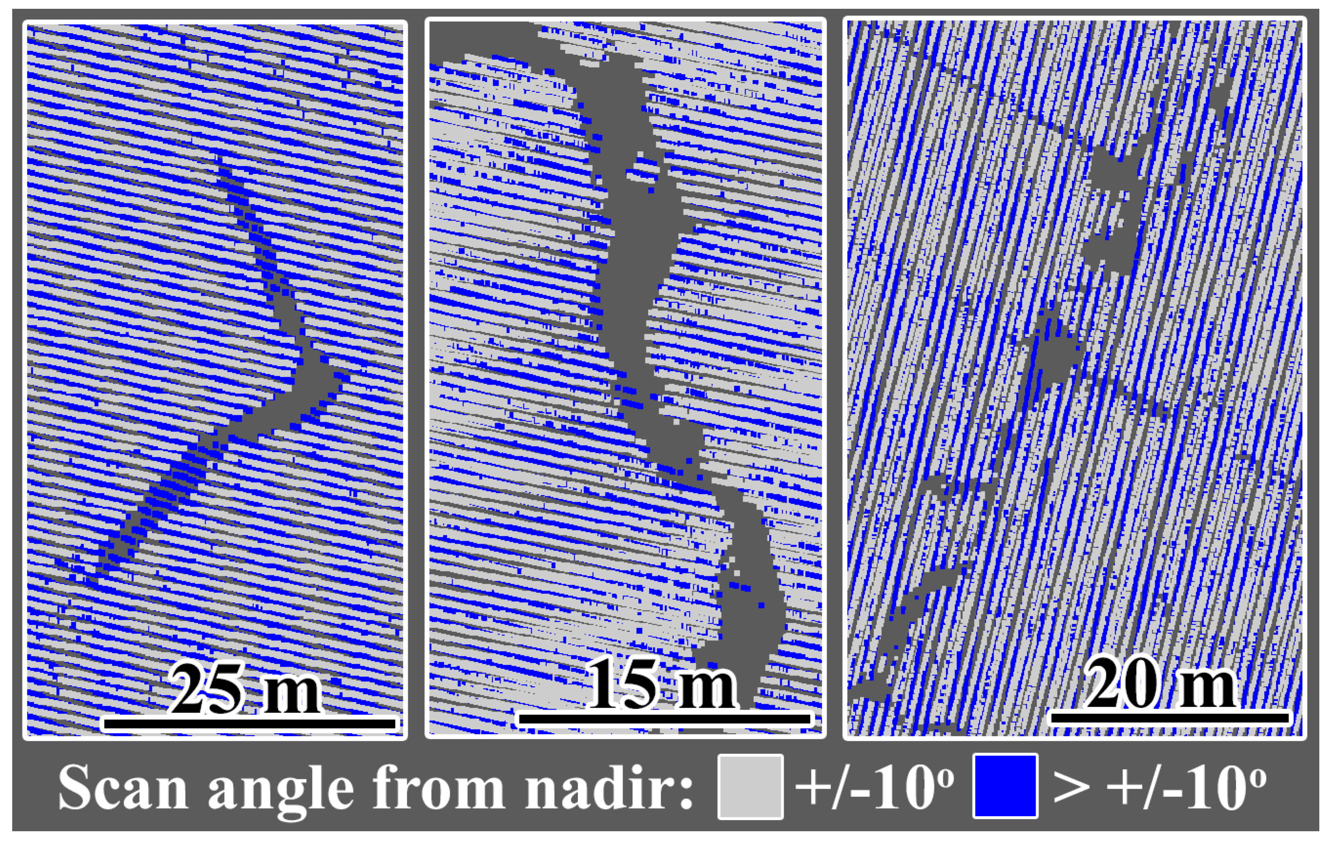
The second factor controlling the representation of creeks and ditches in the airborne lidar data was the scan-angles of available observations. The structure, and even the presence of some creeks and ditches were only observable at scan-angles of ±10° of nadir (Figure 18). Although G-LiHT’s swath width is 387 m at its typical operational altitude of 355 m the requirement of blanket coverage at ±10° of nadir would mean that there should only be a maximum distance of 125.2 m between flight-lines in future acquisitions. Since this would increase the number of flight-lines to cover a saltmarsh, and therefore the cost of deployment, and since G-LiHT’s airborne lidar was able to capture creeks and ditches competently in these acquisitions, further investigation is warranted before changing the flight line protocol for future studies. Additionally, increases in the resolution of the lidar data from G-LiHT are expected in the future, owing to the addition of a second identical lidar instrument, which should improve characterization of creeks and ditches. It is worth noting that since the classification model relies on the presence of below-platform returns to eventually classify a partition as a ditch, it may also be improved by a change in waveform processing, or access to full-waveform observations.
Analyzing the density of the airborne lidar observations implies that higher resolution data products could be produced from future G-LiHT acquisitions, and possibly even derived from the existing datasets (Figure 19). A mean observation density of 14.1 pulses/m2 (σ = 5.9) was found in the 2015 lidar acquisitions, with similar observation densities in the 2014 (16.9 pulses/m2, σ = 6.2) and 2016 (15.3 pulses/m2, σ = 6.0) lidar acquisitions. However, there was considerable spatial heterogeneity in the observation densities, mostly associated with the overlap of adjacent fight-lines, where a maximum observation density of 73 pulses/m2 was found. Additionally, since water strongly absorbs the 1550 nm wavelength of the G-LiHT lidar, it is difficult to ascertain whether areas without observations were occluded from view, or were reached by pulses, but reflected insufficient energy to declare a return. With this potentially confounding factor in mind, it seems prudent to implement an observation density assessment that infers the trajectories of pulses [123] before increasing the resolution of the data products. Such an approach mitigates the uncertainty in ecosystems with a high occurrence of water, which is particular important if airborne lidar classifications are to be compared to satellite resources, since water is such an impactful spectral component of cover.
Regardless, lidar characterizations of saltmarsh components will almost always see meaningful improvement as the resolution of available classifications and representations increase. Terrestrial lidar representations of geomorphology were down-sampled to investigate the influence of observation density on tidal modelling. Over a modelled range of tide heights, estimated surface area of water differed greatly (Figure 15) depending on whether the underlying representation of geomorphology was higher resolution (0.25 m) or lower resolution (1 m). That the discrepancy between estimates of water cover derived from high and low resolution geomorphological representations becomes more extreme as tidal height increases (Figure 16, Table A2, Table A3, Table A4 and Table A5) is a pertinent consideration if a lidar model is to be used to interpret satellite observations of saltmarshes, since water coverage estimates will vary most when the magnitude of their influence is greatest. Thus, meaningful improvements to saltmarsh characterization with increased airborne lidar resolution are generally expected, since saltmarsh components tend to exist in relatively pure patches of cover, with convoluted boundaries, and extents in the order of meters. This mosaic-like composition of saltmarshes occurs because of the variation of salinity and topography on a small spatial scale, interacting with the highly specific tolerances, and therefore niches, of vegetation types, and is one of the major motivations for using airborne lidar for monitoring.
The tendency towards improved water cover estimates with improved representations of geomorphology also strongly recommends higher resolution retrievals of geomorphology for future airborne lidar surveys of saltmarshes. However, an additional overflight in the late winter or early spring would likely be required, when vegetation is absent from the creeks and ditches. Additionally, capturing features of creeks and ditches below the marsh platform might require adjustments to flight-line spacing to mitigate occlusion outside of ±10° of nadir, as previously discussed. Some further justification for these increased logistical costs in future acquisitions is provided, since the benefits to interpreting satellite signals when tidal models are used with high resolution geomorphology are demonstrated. Embedding a water cover estimate derived from terrestrial lidar modelling of geomorphology into the 2015 classification map derived from airborne lidar improved the prediction of Landsat 8 reflectance by 9.59% for green (+9.29% remaining error), 14.2% for red (+4.2% remaining error), and 3.38% for NIR (−0.12% remaining error). Although this example seems very successful, it should be noted that this is only for a single sample Landsat pixel, selected for prominently featuring a creek, and therefore does not have the validation or scope of inference to be considered as more than a demonstration of the method.
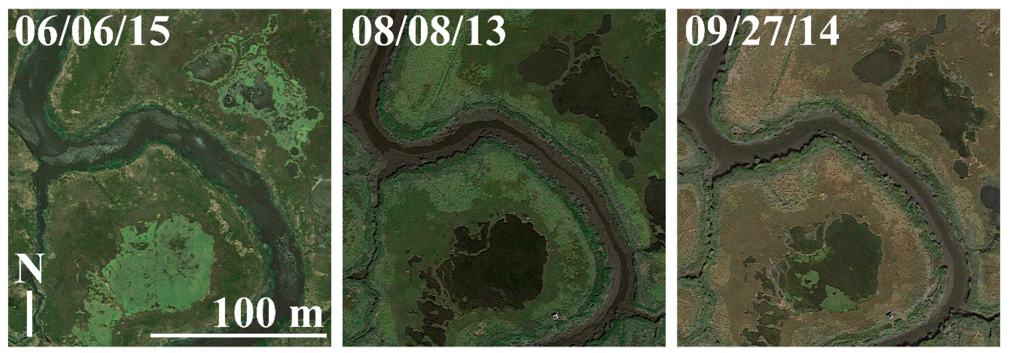
The ability to observe the algae present in the saltmarsh pannes was also found to be dependent on view-angle. Airborne lidar classifications in 2015 were able to capture the presence of algae in the pannes reliably from angles ±15°, but there were often no lidar returns from the algae at larger incidence angles (Figure 14), likely due to energy absorption from the water content of the algae and panne, and the lower returning energy from these more acute incidence angle. Spectroscopy measurements taken in situ suggested that the algae is quite spectrally distinct from other vegetated platform components and the water beneath it (Figure 4), and historical high resolution imagery speaks both to the conservation of the presence and shape of the pannes, and the intra- and inter-annual variation in algal cover (Figure 20). Aerial imagery from June 2013 suggests extremely low algae coverage in the same set of pannes which are confirmed by aerial imagery and the airborne lidar to be mostly covered in algae in June 2015 (estimated at 81.6% by airborne lidar).
Since the algae is a spectrally distinct saltmarsh component, and appears to vary on timescales different to the general marsh platform phenology, it is important to consider its retrieval in future airborne lidar acquisitions. The ability to delineate algae by its intensity in lidar returns would facilitate filtering it out from future estimates of standing water, but to study the algae in its own right would require G-LiHT to operate with a distance no greater than 190.25 m between flight-lines, given its 355 m typical operational altitude.
For pannes themselves, airborne lidar-derived estimates of water extent (including area classified as algae) were close to those derived from terrestrial lidar (+11.2%) for a convoluted area of pannes (Figure 14). Pannes are particularly appealing to characterize across wider scales in New England saltmarshes since they harbor unique microalgal communities [124], and may be vulnerable to perturbation by changing conditions including sea-level rise, and the legacy of anthropogenic modification of hydrological features [125,126]. G-LiHT appeared to effectively represent pannes in all three years of acquisitions, and so proceeding with the current protocol and deployment specifications is expected to be appropriate for future studies.
An attempt was also made to classify wrack using the intensity of lidar returns. The 2015 airborne lidar classification showed favorable results in comparison to contemporary aerial imagery (Figure 9). However, propagating the threshold of intensity used to classify wrack in the 2015 airborne lidar to the lidar acquisitions from the other years made it apparent that it was too sensitive a threshold for the 2014 acquisitions, and vastly too sensitive for the 2016 acquisitions. Ground spectroscopy measurements of wrack suggested that its reflectivity can be highly variable (Figure 4), possibly related to the species of the dead vegetation, and its saturation state. Since iteration of the intensity threshold did not produce wrack retrievals for the 2014 and 2016 acquisitions that were of comparable quality to the 2015 retrieval this is a subject that warrants further study. If future deployments of G-LiHT are conducted under suitable atmospheric conditions, then the onboard hyperspectral instrument may provide more insight into the spectral signature of wrack, and conceivably provide competent wrack classifications on its own.
4.2. Limitations of the Study
4.2.1. Validation
The advantage of airborne lidar as a survey tool is that it can achieve wide structural coverage at relatively high resolutions. Inevitably, obtaining meaningful validation data at similar scales and resolutions is challenging. There were several sources of observations available to corroborate findings, including aerial imagery and terrestrial lidar. However, the terrestrial lidar data were limited in extent, and the areas surveyed with terrestrial lidar were not randomly selected within the airborne lidar survey area, limiting their scope of inference. Additionally, the aerial imagery was separated from the airborne lidar acquisitions by weeks or months for the 2014 and 2016 acquisitions, leading to considerable uncertainty in whether they were representative of conditions during the airborne lidar acquisitions. For the 2015 airborne lidar acquisitions, aerial imagery was available from within three days, but these aerial images were consulted during the process of parameterizing the classification model, and therefore cannot be considered as true validation.
These limitations in validation caution against putting the classification and characterization methods, along with their parameterization, into immediate operational use for wider-scale surveys, particularly if the results from such surveys would sway ecosystem management decisions. However, as a pathfinding effort to produce operational models in the future, promising approaches have been demonstrated for many of the prominent components of northeastern saltmarshes. Independently parameterizing the models, without reference to external sources and accompanied by robust validation, will be the natural next step. In addition, adaption or expansion of the methods may be needed for their application to saltmarshes from other, distinct regions.
4.2.2. Precedence in Classifications
The classification model gives precedence to certain components over others. For example, water can only be recorded as the classification for a partition if there were no lidar returns in the partition, so any form of mixed cover within the partition will result in a classification other than water. This effect is visible in the underrepresentation of water by the airborne classification. An opposite case is Phragmites australis, which will be classified in any partition with maximum heights of lidar returns above 1 m, although this classification is, in turn, supplanted by a classification of trees if there are lidar returns above 3 m in height. The net effect of these mechanisms is the relative dilation of patches of the components that are given precedence in the classification model, and therefore the potential to overestimate their extent. By extension, classifications that are not given precedence will have a tendency towards underestimation. These tendencies will be exacerbated as the resolution of classifications decrease and the size of partitions increase.
Ultimately, classification models always have to make a choice in cases where a partition has symptoms of multiple classifications, and the rule that governs that choice will introduce an accompanying bias. The implementation of these rules should be guided by knowledge of which type of error it is most important to mitigate in a given study. For example, for a management decision that is dependent on a classification model, if it would be more detrimental for a particular component to be underestimated by false negatives, then the rules and parameterization of the classification model should govern in favor of that particular classification in uncertain cases. Since this study was seeking to assess the general capabilities of airborne lidar as a survey tool for saltmarshes, such considerations were not applied in the formation and parameterization of the classification model. However, these factors should be considered in the interpretation of the results.
4.2.3. Scope of Inference
While airborne lidar is demonstrated capturing Phragmites australis and the tall Spartina alterniflora, it should be noted that this capability arises from the distinct height difference between these species and the other marsh platform vegetation. Although the marsh platform is dominated by Spartina patens and the short form of Spartina alterniflora, these species were not able to be separated from each other by height. Neither could other genera present in the marsh platform be distinguished by height, such as Distichlis, Limonium, Salicornia, and Solidago. Therefore, while this study suggests airborne lidar could be effective for estimating coverage of some species, across this particular region of saltmarshes, this success may not propagate to other regions where height differences are less distinct between components. In addition, saltmarshes with greater structural complexity, where vegetation topography varies over distances shorter than the airborne lidar footprint could be challenging, and structural delineation might be achieved more readily with polarimetric SAR.
5. Conclusions
The potential of small-footprint airborne lidar data to characterize ecologically significant components of saltmarshes was explored by using NASA Goddard’s Lidar, Hyperspectral and Thermal (G-LiHT). Airborne lidar retrievals were made with G-LiHT in a well-studied National Science Foundation (NSF) Long Term Ecological Research (LTER) site in Plum Island (Massachusetts, United States) in 2014, 2015 and 2016, along with complimentary terrestrial lidar acquisitions and ground spectroscopy measurements. Classifications of vegetation type, creeks, ditches, pools and pannes, estimates of the spread of the invasive reed Phragmites australis, and the volume of Spartina alterniflora on creek banks were retrieved from the airborne lidar data. The classifications based on observable structure from airborne lidar classifications were encouraging when evaluated through comparisons to airborne imagery and terrestrial lidar. Classifications of wrack (dead, detached vegetation), based on airborne lidar intensities, were successful in the 2015 dataset. However, the thresholds in intensity did not propagate successfully to the 2014 and 2016 dataset, warranting further investigation. Classifications of algae, also based on lidar intensity, were found to depend on observation angles close to nadir, as were observations of the structure and vegetation below the height of the marsh platform, in ditches and creeks.
Airborne lidar is confirmed by these findings to be an effective saltmarsh survey tool, and has the potential to provide information to refine and extend interpretations of saltmarshes from long-term satellite resources. Some of the remaining challenges to the airborne lidar characterizations may well be met by spectral instruments in the G-LiHT package, as well as improvements to G-LiHT, including the addition of a second lidar and an improved GNSS/INS, that have already occurred since the conclusion of this study. If appropriate overflight conditions can be met, lidar classification models may also be refined by the hyperspectral and thermal instruments. The G-LiHT hyperspectral instrument could be particularly useful for further delineating genera of vegetation within the marsh platform, including Spartina, Distichlis, Limonium, Salicornia, and Solidago, as well as identifying any upland species at the saltmarsh edge. The addition of an identical lidar instrument should increase the density of observations, and therefore improve estimates of cover extent in future acquisitions. A newly integrated Phase One digital camera on G-LiHT now offers RGB imagery at a resolution of approximately 3 cm on the ground, which will offer excellent corroborating and contextualizing information, as well as the potential for even higher resolution classifications. Finally, the recently upgraded INS/GNSS unit should enable high confidence in the geolocation and co-location of future acquisitions, which was identified as essential for classification efforts with airborne lidar.
To finalize operational models for wider-scale surveys of northeastern saltmarshes, future studies should expand and formalize validation. Tools such as Unmanned Airborne Vehicles (UAVs) could be used to expand validation efforts, though UAVs would have to leverage their flexible logistics to meet the challenge of the frequently windy conditions in these coastal ecosystems. Including hyperspectral imagery among the ground acquisitions supporting overflights could help the integration of G-LiHT hyperspectral observations, as well as providing further insight into the relationship between airborne and multispectral satellite observations. The spectral influence and variation of the tidal water found in the creeks and ditches, and the standing water found in the pools and pannes is another important bridge to be made between ground, airborne, and satellite observations.
The synthesis of airborne lidar and terrestrial lidar produced some favorable results. However, since terrestrial lidar coverage will always be limited in extent in comparison to airborne lidar, these results speak more to the potential benefit from additional retrievals of airborne lidar during later winter or early spring, when vegetation would be absent from the marsh platform. Also, specifications were offered for future airborne acquisitions seeking to best characterize certain components, such as the requirements for flight-line spacing for the retrieval of algae extent and geomorphological structure.
Overall, this multi-year study can help plan effective regional-scale surveys of saltmarshes by utilizing the ever-improving G-LiHT instrument package, as well as providing insight for others seeking to do the same with similar airborne remote sensing resources in other regions. The ever-lengthening satellite record, and ever-improving available satellite resources, especially the publically available Landsat and Sentinel series, are the best tools for monitoring long-term change in saltmarsh ecosystems. Airborne lidar retrievals were evaluated in this context, finding that the active technology has a great deal to offer to the refinement and interpretation of satellite passive observations. Airborne lidar acquisitions stand to be especially beneficial to satellite monitoring of saltmarshes if the airborne acquisitions are carefully targeted to capture the most informative windows of phenological and tidal state. It is also apparent that multiple acquisitions at key times in a single year, in particular when vegetation is absent, and when it is at peak growth, will be worth more than the sum of their parts. G-LiHT, even functioning as it was here solely as a source of discrete airborne lidar data, performed well in retrieving important saltmarsh components, and it is clear that there remains much untapped potential for characterizing saltmarshes in the wider G-LiHT instrument package, and airborne lidar in general.
Author Contributions
Conceptualization, I.P., C.S., and B.C.; methodology, I.P., C.S., and B.C.; software, I.P. and F.P.; validation, I.P.; formal analysis, I.P.; investigation, I.P., C.S., and B.C.; resources, C.S., F.P., J.L.B., L.D., and B.C.; data curation, I.P., C.S., and B.C.; writing—original draft preparation, I.P.; writing—review and editing, C.S., J.L.B., L.D.; visualization, I.P.; supervision, C.S., J.L.B., L.D., and B.C.; project administration, C.S. and B.C.; funding acquisition, C.S. and B.C.
Funding
This research was funded by the Oracle Graduate Fellowship, and NASA grant numbers NNX14AK12G and NNX14AI73G.
Acknowledgments
For facilitating work at Plum Island: Anne Giblin (Lead PI PIE LTER), members of PIE LTER, and members of TIDE Project. For fieldwork, and data collection and processing assistance: Edward Saenz, Daniel Genest, Angela Erb, Zhan Li, Qingsong Sun, Shabnam Rouhani, Yan Liu, Kara Wiggin, Christina Ciarfella, Erica Skye Schaaf, Jack Payette, Molly Forgaard, Randall Erb, Lawrence Corp. For advice: Patrick Kearns, Robert Chen, Alan Strahler, Sergio Fagherazzi, David Johnson.
Conflicts of Interest
The authors declare no conflict of interest.
Appendix A

Table A1.
Phragmites australis growth from terrestrial lidar acquisitions throughout 2015. Volumes rounded to two decimal places.
Table A1.
Phragmites australis growth from terrestrial lidar acquisitions throughout 2015. Volumes rounded to two decimal places.
| Date (dd/mm/yy) | Total Area (m2) | Additional Area (m2) | Total Volume (m3) | Additional Volume (m3) |
|---|---|---|---|---|
| 05/14/15 | 1183.25 | 0 | 223.05 | 0 |
| 05/24/15 | 1439 | 255.75 | 311.02 | 87.97 |
| 06/04/15 | 1643.5 | 204.5 | 382.61 | 71.59 |
| 06/10/15 | 1756.25 | 112.75 | 423.52 | 40.91 |
| 06/17/15 | 1861 | 104.75 | 471.51 | 47.99 |
| 06/25/15 | 1915.5 | 54.5 | 506.47 | 34.96 |
| 07/03/15 | 1954.25 | 38.75 | 544.54 | 38.07 |
| 07/11/15 | 2042.75 | 88.5 | 578.68 | 34.13 |
| 07/19/15 | 2151.5 | 108.75 | 642.46 | 63.78 |
| 08/12/15 | 2230.25 | 78.75 | 678.89 | 36.43 |
| 08/28/15 | 2265.5 | 35.25 | 726.83 | 47.94 |
| 09/21/15 | 2343 | 77.5 | 770.52 | 43.69 |
| 10/15/15 | 2398.25 | 55.25 | 811.55 | 41.03 |
| 11/15/15 | 2500.25 | 102 | 899.32 | 87.76 |
Table A2.
Creek A Volume (m3) from Terrestrial Lidar, rounded to two decimal places.
| Height of Water (m) | Resolution (m) | ||
|---|---|---|---|
| 0.25 | 0.5 | 1 | |
| 2.5 | 1119.68 | 1048.08 | 922.09 |
| 2.25 | 907.27 | 829.66 | 693.05 |
| 2 | 713.01 | 641.74 | 514.69 |
| 1.75 | 563.86 | 503.95 | 393.58 |
| 1.5 | 440.77 | 390.52 | 295.95 |
| 1.25 | 335.48 | 294.26 | 215.63 |
| 1 | 245.04 | 212.29 | 148.95 |
| 0.75 | 165.40 | 140.54 | 92.34 |
| 0.5 | 97.97 | 81.00 | 48.39 |
| 0.25 | 43.49 | 34.54 | 17.89 |
Table A3.
Creek B Volume (m3) from Terrestrial Lidar, rounded to two decimal places.
| Height of Water (m) | Resolution (m) | ||
|---|---|---|---|
| 0.25 | 0.5 | 1 | |
| 2.5 | 901.70 | 845.42 | 769.99 |
| 2.25 | 678.63 | 616.71 | 530.15 |
| 2 | 472.10 | 404.61 | 312.73 |
| 1.75 | 308.23 | 251.20 | 176.12 |
| 1.5 | 191.01 | 144.29 | 86.57 |
| 1.25 | 115.05 | 78.18 | 37.16 |
| 1 | 67.48 | 40.26 | 14.54 |
| 0.75 | 39.81 | 21.27 | 6.34 |
| 0.5 | 22.23 | 11.36 | 3.00 |
| 0.25 | 10.01 | 4.98 | 1.25 |
Table A4.
Creek A Surface Area (m2) from Terrestrial Lidar.
| Height of Water (m) | Resolution (m) | ||
|---|---|---|---|
| 0.25 | 0.5 | 1 | |
| 2.5 | 162.25 | 112.5 | 158 |
| 2.25 | 193.25 | 174 | 238 |
| 2 | 242.50 | 253.5 | 313 |
| 1.75 | 295.50 | 314.5 | 370 |
| 1.5 | 340.25 | 387.5 | 430 |
| 1.25 | 391.75 | 460.5 | 495 |
| 1 | 459 | 558.5 | 584 |
| 0.75 | 539.50 | 660.5 | 701 |
| 0.5 | 692.50 | 835.5 | 868 |
| 0.25 | 903.25 | 914.5 | 958 |
Table A5.
Creek B Surface Area (m2) from Terrestrial Lidar.
| Height of Water (m) | Resolution (m) | ||
|---|---|---|---|
| 0.25 | 0.5 | 1 | |
| 2.5 | 28 | 1 | 6 |
| 2.25 | 31 | 9 | 25 |
| 2 | 46.25 | 34.5 | 69 |
| 1.75 | 78.25 | 98.5 | 131 |
| 1.5 | 130.75 | 188.5 | 215 |
| 1.25 | 253 | 317 | 344 |
| 1 | 360.5 | 483 | 507 |
| 0.75 | 587.75 | 669 | 731 |
| 0.5 | 718.75 | 831.5 | 882 |
| 0.25 | 887.25 | 928.5 | 993 |
References
- Frey, R.W.; Basan, P.B. Coastal salt marshes. In Coastal Sedimentary Environments; Springer: New York, NY, USA, 1978; pp. 101–169. [Google Scholar]
- Allen, J.R.L. Morphodynamics of Holocene salt marshes: A review sketch from the Atlantic and Southern North Sea coasts of Europe. Quat. Sci. Rev. 2000, 19, 1155–1231. [Google Scholar] [CrossRef]
- Ranwell, D.S. Ecology of Salt Marshes and Sand Dunes; Chapman and Hall: London, UK, 1972; Volume 258. [Google Scholar]
- Duarte, B.; Reboreda, R.; Caçador, I. Seasonal variation of extracellular enzymatic activity (EEA) and its influence on metal speciation in a polluted salt marsh. Chemosphere 2008, 73, 1056–1063. [Google Scholar] [CrossRef] [PubMed]
- Adams, D.A. Factors influencing vascular plant zonation in North Carolina salt marshes. Ecology 1963, 44, 445–456. [Google Scholar] [CrossRef]
- Costa, C.S.; Marangoni, J.C.; Azevedo, A.M. Plant zonation in irregularly flooded salt marshes: Relative importance of stress tolerance and biological interactions. J. Ecol. 2003, 91, 951–965. [Google Scholar] [CrossRef]
- Pennings, S.C.; Grant, M.B.; Bertness, M.D. Plant zonation in low-latitude salt marshes: Disentangling the roles of flooding, salinity and competition. J. Ecol. 2005, 93, 159–167. [Google Scholar] [CrossRef]
- Mcleod, E.; Chmura, G.L.; Bouillon, S.; Salm, R.; Björk, M.; Duarte, C.M.; Lovelock, C.E.; Schlesinger, W.H.; Silliman, B.R. A blueprint for blue carbon: Toward an improved understanding of the role of vegetated coastal habitats in sequestering CO2. Front. Ecol. Environ. 2011, 9, 552–560. [Google Scholar] [CrossRef]
- Howard, J.; Hoyt, S.; Isensee, K.; Telszewski, M.; Pidgeon, E. Coastal Blue Carbon: Methods for Assessing Carbon Stocks and Emissions Factors in Mangroves, Tidal Salt Marshes, and Seagrasses; Conservation International, Intergovernmental Oceanographic Commission of UNESCO, International Union for Conservation of Nature: Arlington, VA, USA, 2014. [Google Scholar]
- Feagin, R.A.; Lozada-Bernard, S.M.; Ravens, T.M.; Möller, I.; Yeager, K.M.; Baird, A.H. Does vegetation prevent wave erosion of salt marsh edges? Proc. Natl. Acad. Sci. USA 2009, 106, 10109–10113. [Google Scholar] [CrossRef] [PubMed] [Green Version]
- Möller, I.; Spencer, T. Wave dissipation over macro-tidal saltmarshes: Effects of marsh edge typology and vegetation change. J. Coast. Res. 2002, 36, 506–521. [Google Scholar] [CrossRef]
- Nixon, S.W. Between Coastal Marshes and Coastal Waters—A Review of Twenty Years of Speculation and Research on the Role of Salt Marshes in Estuarine Productivity and Water Chemistry; Springer: New York, NY, USA, 2012; pp. 437–525. [Google Scholar]
- Connor, R.F.; Chmura, G.L.; Beecher, C.B. Carbon accumulation in Bay of Fundy salt marshes: Implications for restoration of reclaimed marshes. Glob. Biogeochem. Cycles 2001, 15, 943–954. [Google Scholar] [CrossRef]
- Chmura, G.L.; Anisfeld, S.C.; Cahoon, D.R.; Lynch, J.C. Global carbon sequestration in tidal, saline wetland soils. Glob. Biogeochem. Cycles 2003, 17. [Google Scholar] [CrossRef]
- Pendleton, L.; Donato, D.C.; Murray, B.C.; Crooks, S.; Jenkins, W.A.; Sifleet, S.; Craft, C.; Fourqurean, J.W.; Kauffman, J.B.; Marbà, N.; Megonigal, P. Estimating global “blue carbon” emissions from conversion and degradation of vegetated coastal ecosystems. PloS ONE 2012, 7, 43542. [Google Scholar] [CrossRef] [PubMed]
- Möller, I.; Spencer, T.; French, J.R.; Leggett, D.J.; Dixon, M. The Sea-Defence Value of Salt Marshes: Field Evidence From North Norfolk. Water Environ. J. 2001, 15, 109–116. [Google Scholar] [CrossRef]
- Möller, I.; Spencer, T.; French, J.R.; Leggett, D.J.; Dixon, M. Wave transformation over salt marshes: A field and numerical modelling study from North Norfolk, England. Estuar. Coast. Shelf Sci. 1999, 49, 411–426. [Google Scholar] [CrossRef]
- Thorne, K.M.; Takekawa, J.Y.; Elliott-Fisk, D.L. Ecological effects of climate change on salt marsh wildlife: A case study from a highly urbanized estuary. J. Coast. Res. 2012, 28, 1477–1487. [Google Scholar] [CrossRef]
- Wilson, A.M.; Moore, W.S.; Joye, S.B.; Anderson, J.L.; Schutte, C.A. Storm-driven groundwater flow in a salt marsh. Water Resour. Res. 2011, 47. [Google Scholar] [CrossRef] [Green Version]
- Valiela, I.; Cole, M.L. Comparative evidence that salt marshes and mangroves may protect seagrass meadows from land-derived nitrogen loads. Ecosystems 2002, 5, 92–102. [Google Scholar] [CrossRef]
- Cao, Y.; Green, P.G.; Holden, P.A. Microbial community composition and denitrifying enzyme activities in salt marsh sediments. Appl. Environ. Microbiol. 2008, 74, 7585–7595. [Google Scholar] [CrossRef] [PubMed]
- Boesch, D.F.; Turner, R.E. Dependence of fishery species on salt marshes: The role of food and refuge. Estuaries 1984, 7, 460–468. [Google Scholar] [CrossRef]
- Irlandi, E.A.; Crawford, M.K. Habitat linkages: The effect of intertidal saltmarshes and adjacent subtidal habitats on abundance, movement, and growth of an estuarine fish. Oecologia 1997, 110, 222–230. [Google Scholar] [CrossRef] [PubMed]
- Minello, T.J.; Able, K.W.; Weinstein, M.P.; Hays, C.G. Salt marshes as nurseries for nekton: Testing hypotheses on density, growth and survival through meta-analysis. Mar. Ecol. Prog. Ser. 2003, 246, 39–59. [Google Scholar] [CrossRef]
- Green, B.C.; Smith, D.J.; Grey, J.; Underwood, G.J. High site fidelity and low site connectivity in temperate salt marsh fish populations: A stable isotope approach. Oecologia 2012, 168, 245–255. [Google Scholar] [CrossRef] [PubMed]
- Burger, J.; Shisler, J.; Lesser, F.H. Avian utilisation on six salt marshes in New Jersey. Biol. Conserv. 1982, 23, 187–212. [Google Scholar] [CrossRef]
- Bos, D.; Loonen, M.J.; Stock, M.; Hofeditz, F.; Van der Graaf, A.J.; Bakker, J.P. Utilisation of Wadden Sea salt marshes by geese in relation to livestock grazing. J. Nat. Conserv. 2005, 13, 1–15. [Google Scholar] [CrossRef] [Green Version]
- Tian, B.; Zhou, Y.; Zhang, L.; Yuan, L. Analyzing the habitat suitability for migratory birds at the Chongming Dongtan Nature Reserve in Shanghai, China. Estuar. Coast. Shelf Sci. 2008, 80, 296–302. [Google Scholar] [CrossRef]
- Beaumont, N.J.; Austen, M.C.; Mangi, S.C.; Townsend, M. Economic valuation for the conservation of marine biodiversity. Mar. Pollut. Bull. 2008, 56, 386–396. [Google Scholar] [CrossRef] [PubMed]
- Allen John, R.L. Saltmarshes: Morphodynamics, Conservation, and Engineering Significance; Cambridge University Press: Cambridge, UK, 1992. [Google Scholar]
- Simas, T.; Nunes, J.P.; Ferreira, J.G. Effects of global climate change on coastal salt marshes. Ecol. Model. 2001, 139, 1–15. [Google Scholar] [CrossRef]
- Adam, P. Saltmarshes in a time of change. Environ. Conserv. 2002, 29, 39–61. [Google Scholar] [CrossRef]
- Wigand, C.; McKinney, R.A.; Charpentier, M.A.; Chintala, M.M.; Thursby, G.B. Relationships of nitrogen loadings, residential development, and physical characteristics with plant structure in New England salt marshes. Estuaries 2003, 26, 1494–1504. [Google Scholar] [CrossRef]
- Deegan, L.A.; Bowen, J.L.; Drake, D.; Fleeger, J.W.; Friedrichs, C.T.; Galvan, K.A.; Hobbie, J.E.; Hopkinson, C.; Johnson, D.S.; Johnson, J.M.; et al. Susceptibility of salt marshes to nutrient enrichment and predator removal. Ecol. Appl. 2007, 17. [Google Scholar] [CrossRef]
- Turner, R.E.; Howes, B.L.; Teal, J.M.; Milan, C.S.; Swenson, E.M.; Goehringer-Toner, D.D. Salt marshes and eutrophication: An unsustainable outcome. Limnol. Oceanogr. 2009, 54, 1634. [Google Scholar] [CrossRef]
- Lin, Q.; Mendelssohn, I.A. A comparative investigation of the effects of south Louisiana crude oil on the vegetation of fresh, brackish and salt marshes. Mar. Pollut. Bull. 1996, 32, 202–209. [Google Scholar] [CrossRef]
- Mason, C.F.; Underwood, G.J.C.; Baker, N.R.; Davey, P.A.; Davidson, I.; Hanlon, A.; Long, S.P.; Oxborough, K.; Paterson, D.M.; Watson, A. The role of herbicides in the erosion of salt marshes in eastern England. Environ. Pollut. 2003, 122, 41–49. [Google Scholar] [CrossRef]
- Bai, J.; Xiao, R.; Zhang, K.; Gao, H. Arsenic and heavy metal pollution in wetland soils from tidal freshwater and salt marshes before and after the flow-sediment regulation regime in the Yellow River Delta, China. J. Hydrol. 2012, 450, 244–253. [Google Scholar] [CrossRef]
- Silliman, B.R.; van de Koppel, J.; McCoy, M.W.; Diller, J.; Kasozi, G.N.; Earl, K.; Adams, P.N.; Zimmerman, A.R. Degradation and resilience in Louisiana salt marshes after the BP–Deepwater Horizon oil spill. Proc. Natl. Acad. Sci. USA 2012, 109, 11234–11239. [Google Scholar] [CrossRef] [PubMed]
- Bolivar, J.P.; García-Tenorio, R.; García-León, M. Enhancement of natural radioactivity in soils and salt-marshes surrounding a non-nuclear industrial complex. Sci. Total Environ. 1995, 173, 125–136. [Google Scholar] [CrossRef]
- Thomson, J.; Dyer, F.M.; Croudace, I.W. Records of radionuclide deposition in two salt marshes in the United Kingdom with contrasting redox and accumulation conditions. Geochim. Cosmochim. Acta 2002, 66, 1011–1023. [Google Scholar] [CrossRef]
- Reed, D.J. The impact of sea-level rise on coastal salt marshes. Prog. Phys. Geogr. 1990, 14, 465–481. [Google Scholar] [CrossRef]
- Van Wijnen, H.J.; Bakker, J.P. Long-term surface elevation change in salt marshes: A prediction of marsh response to future sea-level rise. Estuar. Coast. Shelf Sci. 2001, 52, 381–390. [Google Scholar] [CrossRef]
- Ranwell, D.S. Spartina salt marshes in southern England: I. The effects of sheep grazing at the upper limits of Spartina marsh in Bridgwater Bay. J. Ecol. 1961, 325–340. [Google Scholar] [CrossRef]
- Morris, J.T.; Jensen, A. The carbon balance of grazed and non-grazed Spartina anglica saltmarshes at Skallingen, Denmark. J. Ecol. 1998, 86, 229–242. [Google Scholar] [CrossRef] [Green Version]
- Silliman, B.R.; Bertness, M.D. Shoreline development drives invasion of Phragmites australis and the loss of plant diversity on New England salt marshes. Conserv. Biol. 2004, 18, 1424–1434. [Google Scholar] [CrossRef]
- Hartig, E.K.; Gornitz, V.; Kolker, A.; Mushacke, F.; Fallon, D. Anthropogenic and climate-change impacts on salt marshes of Jamaica Bay, New York City. Wetlands 2002, 22, 71–89. [Google Scholar] [CrossRef]
- Gedan, K.B.; Altieri, A.H.; Bertness, M.D. Uncertain future of New England salt marshes. Mar. Ecol. Prog. Ser. 2011, 434, 229–237. [Google Scholar] [CrossRef]
- Burdick, D.M.; Buchsbaum, R.; Holt, E. Variation in soil salinity associated with expansion of Phragmites australis in salt marshes. Environ. Exp. Bot. 2001, 46, 247–261. [Google Scholar] [CrossRef]
- Bart, D.; Hartman, J.M. The role of large rhizome dispersal and low salinity windows in the establishment of common reed, Phragmites australis, in salt marshes: New links to human activities. Estuaries 2003, 26, 436–443. [Google Scholar] [CrossRef]
- Vasquez, E.A.; Glenn, E.P.; Brown, J.J.; Guntenspergen, G.R.; Nelson, S.G. Salt tolerance underlies the cryptic invasion of North American salt marshes by an introduced haplotype of the common reed Phragmites australis (Poaceae). Mar. Ecol. Prog. Ser. 2005, 298, 1–8. [Google Scholar] [CrossRef] [Green Version]
- Gedan, K.B.; Silliman, B.R.; Bertness, M.D. Centuries of human-driven change in salt marsh ecosystems. Mar. Sci. 2009, 1, 117–141. [Google Scholar] [CrossRef] [PubMed]
- Green, E.P.; Mumby, P.J.; Edwards, A.J.; Clark, C.D. A review of remote sensing for the assessment and management of tropical coastal resources. Coast. Manag. 1996, 24, 1–40. [Google Scholar] [CrossRef] [Green Version]
- Malthus, T.J.; Mumby, P.J. Remote sensing of the coastal zone: An overview and priorities for future research. Int. J. Remote Sens. 2003, 24, 2805–2815. [Google Scholar] [CrossRef] [Green Version]
- Gallant, A. The Challenges of remote monitoring of wetlands. Remote Sens. 2015, 7, 10938–10950. [Google Scholar] [CrossRef]
- Williams, P.B.; Orr, M.K. Physical evolution of restored breached levee salt marshes in the San Francisco Bay estuary. Restor. Ecol. 2002, 10, 527–542. [Google Scholar] [CrossRef]
- Schuerch, M.; Vafeidis, A.; Slawig, T.; Temmerman, S. Modeling the influence of changing storm patterns on the ability of a salt marsh to keep pace with sea level rise. J. Geophys. Res. Earth Surf. 2013, 118, 84–96. [Google Scholar] [CrossRef] [Green Version]
- Guo, M.; Li, J.; Sheng, C.; Xu, J.; Wu, L. A review of wetland remote sensing. Sensors 2017, 17, 777. [Google Scholar] [CrossRef] [PubMed]
- Wang, C.; Menenti, M.; Stoll, M.P.; Feola, A.; Belluco, E.; Marani, M. Separation of ground and low vegetation signatures in LiDAR measurements of salt-marsh environments. IEEE Trans. Geosci. Remote Sens. 2009, 47, 2014–2023. [Google Scholar] [CrossRef]
- Moeslund, J.E.; Arge, L.; Bøcher, P.K.; Nygaard, B.; Svenning, J.C. Geographically comprehensive assessment of salt-meadow vegetation-elevation relations using LiDAR. Wetlands 2011, 31, 471–482. [Google Scholar] [CrossRef]
- Hladik, C.; Alber, M. Classification of salt marsh vegetation using edaphic and remote sensing-derived variables. Estuar. Coast. Shelf. Sci. 2014, 141, 47–57. [Google Scholar] [CrossRef]
- Alexander, C.; Deák, B.; Kania, A.; Mücke, W.; Heilmeier, H. Classification of vegetation in an open landscape using full-waveform airborne laser scanner data. Int. J. Appl. Earth Obs. Geoinf. 2015, 41, 76–87. [Google Scholar] [CrossRef]
- Rosso, P.H.; Ustin, S.L.; Hastings, A. Use of lidar to study changes associated with Spartina invasion in San Francisco Bay marshes. Remote Sens. Environ. 2006, 100, 295–306. [Google Scholar] [CrossRef]
- Rapinel, S.; Hubert-Moy, L.; Clément, B. Using LiDAR data to evaluate wetland functions. In Proceedings of the 34th International Symposium for Remote Sensing of the Environment (ISRSE), Sydney, Australia, 10–15 April 2011. [Google Scholar]
- Rapinel, S.; Rossignol, N.; Gore, O.; Jambon, O.; Bouger, G.; Mansons, J.; Bonis, A. Daily Monitoring of Shallow and Fine-Grained Water Patterns in Wet Grasslands Combining Aerial LiDAR Data and In Situ Piezometric Measurements. Sustainability 2018, 10, 708. [Google Scholar] [CrossRef]
- Schalles, J.F.; Hladik, C.M.; Lynes, A.A.; Pennings, S.C. Landscape estimates of habitat types, plant biomass, and invertebrate densities in a Georgia salt marsh. Oceanography 2013, 26, 88–97. [Google Scholar] [CrossRef]
- Rogers, J.N.; Parrish, C.E.; Ward, L.G.; Burdick, D.M. Assessment of Elevation Uncertainty in Salt Marsh Environments using Discrete-Return and Full-Waveform Lidar. J. Coast. Res. 2016, 76 (Suppl. 1), 107–122. [Google Scholar] [CrossRef] [Green Version]
- Hladik, C.; Schalles, J.; Alber, M. Salt marsh elevation and habitat mapping using hyperspectral and LIDAR data. Remote Sens. Environ. 2013, 139, 318–330. [Google Scholar] [CrossRef]
- Montane, J.M.; Torres, R. Accuracy assessment of LIDAR saltmarsh topographic data using RTK GPS. Photogramm. Eng. Remote Sens. 2006, 72, 961–967. [Google Scholar] [CrossRef]
- Wu, Q.; Lane, C.R. Delineating wetland catchments and modeling hydrologic connectivity using lidar data and aerial imagery. Hydrol. Earth Syst. Sci 2017, 21, 3579–3595. [Google Scholar] [CrossRef] [PubMed] [Green Version]
- Rose, L.S.; Seong, J.C.; Ogle, J.; Beute, E.; Indridason, J.; Hall, J.D.; Nelson, S.; Jones, T.; Humphrey, J. Challenges and lessons from a wetland LiDAR project: A case study of the Okefenokee Swamp, Georgia, USA. Geocarto Int. 2013, 28, 210–226. [Google Scholar] [CrossRef]
- Wang, J. (Ed.) Mapping Salt Marsh Vegetation by Integrating Hyperspectral and LiDAR Remote Sensing; CRC Press: Boca Raton, FL, USA, 2009; pp. 173–190. [Google Scholar]
- Rapinel, S.; Hubert-Moy, L.; Clément, B. Combined use of LiDAR data and multispectral earth observation imagery for wetland habitat mapping. Int. J. Appl. Earth Obs. Geoinf. 2015, 37, 56–64. [Google Scholar] [CrossRef]
- Sadro, S.; Gastil-Buhl, M.; Melack, J. Characterizing patterns of plant distribution in a southern California salt marsh using remotely sensed topographic and hyperspectral data and local tidal fluctuations. Remote Sens. Environ. 2007, 110, 226–239. [Google Scholar] [CrossRef]
- Chust, G.; Galparsoro, I.; Borja, A.; Franco, J.; Uriarte, A. Coastal and estuarine habitat mapping, using LIDAR height and intensity and multi-spectral imagery. Estuar. Coast. Shelf Sci. 2008, 78, 633–643. [Google Scholar] [CrossRef]
- Cook, B.D.; Bolstad, P.V.; Næsset, E.; Anderson, R.S.; Garrigues, S.; Morisette, J.T.; Nickeson, J.; Davis, K.J. Using LiDAR and quickbird data to model plant production and quantify uncertainties associated with wetland detection and land cover generalizations. Remote Sens. Environ. 2009, 113, 2366–2379. [Google Scholar] [CrossRef]
- Hladik, C.M.; Alber, M. Salt Marsh Habitat Mapping on Sapelo Island, GA Using LIDAR and Hyperspectral Imagery; Georgia Southern University: Statesboro, GA, USA, 2009. [Google Scholar]
- Wang, J.; Liu, Z.; Yu, H.; Li, F. Mapping Spartina alterniflora Biomass Using LiDAR and Hyperspectral Data. Remote Sens. 2017, 9, 589. [Google Scholar] [CrossRef]
- Kulawardhana, R.W.; Popescu, S.C.; Feagin, R.A. Fusion of lidar and multispectral data to quantify salt marsh carbon stocks. Remote Sens. Environ. 2014, 154, 345–357. [Google Scholar] [CrossRef]
- Collin, A.; Long, B.; Archambault, P. Salt-marsh characterization, zonation assessment and mapping through a dual-wavelength LiDAR. Remote Sens. Environ. 2010, 114, 520–530. [Google Scholar] [CrossRef]
- Van Beijma, S.J. Remote Sensing-Based Mapping and Modelling of Salt Marsh Habitats Based on Optical, Lidar and Sar Data. Ph.D. Thesis, Department of Geography, University of Leicester, Leicester, UK, 2015. Available online: http://hdl.handle.net/2381/32455 (accessed on 15 January 2019).
- Ramsey, E.W.; Nelson, G.A.; Sapkota, S.K. Classifying coastal resources by integrating optical and radar imagery and color infrared photography. Mangroves Salt Marshes 1998, 2, 109–119. [Google Scholar] [CrossRef]
- Ramsey, E., III; Lu, Z.; Rangoonwala, A.; Rykhus, R. Multiple baseline radar interferometry applied to coastal land cover classification and change analyses. Giscience Remote Sens. 2006, 43, 283–309. [Google Scholar] [CrossRef]
- Ramsey, E., III; Rangoonwala, A.; Chi, Z.; Jones, C.E.; Bannister, T. Marsh dieback, loss, and recovery mapped with satellite optical, airborne polarimetric radar, and field data. Remote Sens. Environ. 2014, 152, 364–374. [Google Scholar] [CrossRef]
- Ramsey, E.W., III; Nelson, G.A.; Laine, S.C.; Kirkman, R.G.; Topham, W. Generation of coastal marsh topography with radar and ground-based measurements. J. Coast. Res. 1997, 1335–1341. [Google Scholar]
- Ramsey, E.W., III. Monitoring flooding in coastal wetlands by using radar imagery and ground-based measurements. Int. J. Remote Sens. 1995, 16, 2495–2502. [Google Scholar] [CrossRef]
- Ramsey, E.; Lu, Z.; Suzuoki, Y.; Rangoonwala, A.; Werle, D. Monitoring duration and extent of storm-surge and flooding in western coastal Louisiana marshes with Envisat ASAR data. IEEE J. Sel. Top. Appl. Earth Obs. Remote Sens. 2011, 4, 387–399. [Google Scholar] [CrossRef]
- Suzuoki, Y.; Rangoonwala, A.; Ramsey, E.W., III. Monitoring coastal inundation with Synthetic Aperture Radar satellite data (No. 2011-1208). US Geol. Surv. 2011. [Google Scholar] [CrossRef]
- Ramsey, E.W.; Nelson, G.A.; Sapkota, S.K.; Laine, S.C.; Verdi, J.; Krasznay, S. Using multiple-polarization L-band radar to monitor marsh burn recovery. IEEE Trans. Geosci. Remote Sens. 1999, 37, 635–639. [Google Scholar] [CrossRef]
- Ramsey, E.; Rangoonwala, A.; Middleton, B.; Lu, Z. Satellite optical and radar data used to track wetland forest impact and short-term recovery from Hurricane Katrina. Wetlands 2009, 29, 66. [Google Scholar] [CrossRef]
- Rangoonwala, A.; Enwright, N.M.; Ramsey, E., III; Spruce, J.P. Radar and optical mapping of surge persistence and marsh dieback along the New Jersey Mid-Atlantic coast after Hurricane Sandy. Int. J. Remote Sens. 2016, 37, 1692–1713. [Google Scholar] [CrossRef] [Green Version]
- Ramsey, E.; Rangoonwala, A. Mapping oil in a coastal marsh with polarimetric synthetic aperture radar. Oceans 2012, 1–8. [Google Scholar] [CrossRef]
- Ramsey, E., III; Meyer, B.M.; Rangoonwala, A.; Overton, E.; Jones, C.E.; Bannister, T. Oil source-fingerprinting in support of polarimetric radar mapping of Macondo-252 oil in Gulf Coast marshes. Mar. Pollut. Bull. 2014, 89, 85–95. [Google Scholar] [CrossRef] [PubMed]
- Ramsey, E.; Rangoonwala, A.; Jones, C. Structural classification of marshes with polarimetric SAR highlighting the temporal mapping of marshes exposed to oil. Remote Sens. 2015, 7, 11295–11321. [Google Scholar] [CrossRef]
- Ramsey, E., III; Rangoonwala, A.; Suzuoki, Y.; Jones, C.E. Oil detection in a coastal marsh with polarimetric synthetic aperture radar (SAR). Remote Sens. 2011, 3, 2630–2662. [Google Scholar] [CrossRef]
- Badura, G.P.; Bachmann, C.M.; Tyler, A.C.; Goldsmith, S.; Eon, R.S.; Lapszynski, C.S. A Novel Approach for Deriving LAI of Salt Marsh Vegetation Using Structure From Motion and Multiangular Spectra. IEEE J. Sel. Top. Appl. Earth Obs. Remote Sens. 2019. [Google Scholar] [CrossRef]
- Fernandez-Nunez, M.; Burningham, H.; Zujar, J.O. Improving accuracy of LiDAR-derived digital terrain models for saltmarsh management. J. Coast. Conserv. 2017, 21, 209–222. [Google Scholar] [CrossRef] [Green Version]
- Hodges, B.R. Representing hydrodynamically important blocking features in coastal or riverine lidar topography. Nat. Hazards Earth Syst. Sci. 2015, 15, 1011–1023. [Google Scholar] [CrossRef] [Green Version]
- Hladik, C.; Alber, M. Accuracy assessment and correction of a LIDAR-derived salt marsh digital elevation model. Remote Sens. Environ. 2012, 121, 224–235. [Google Scholar] [CrossRef]
- Chirol, C.; Haigh, I.D.; Pontee, N.; Thompson, C.E.; Gallop, S.L. Parametrizing tidal creek morphology in mature saltmarshes using semi-automated extraction from lidar. Remote Sens. Environ. 2018, 209, 291–311. [Google Scholar] [CrossRef]
- Chapman, V.J. Coastal movement and the development of some New England salt marshes. Proc. Geol. Assoc. 1938, 49, 373–384. [Google Scholar] [CrossRef]
- Deevey, E.S. On the date of the last rise of sea level in southern New England, with remarks on the Grassy Island site. Am. J. Sci. 1948, 246, 329–352. [Google Scholar] [CrossRef]
- Redfield, A.C. Development of a New England salt marsh. Ecol. Monogr. 1972, 42, 201–237. [Google Scholar] [CrossRef]
- Nixon, S.W. Ecol. New Engl. High Salt Marshes: A Community Profile 1982 (No. FWS/OBS-81/55); National Coastal Ecosystems Team: Washington, DC, USA; Rhode Island Univ.: Kingston, RI, USA; Graduate School of Oceanography: Narragansett, RI, USA, 1982. [Google Scholar]
- Teal, J.; Pendleton, E.; Kitchens, W.; Young, M.W. The Ecology of Regularly Flooded Salt Marshes of New England: A Community Profile; Fish and Wildlife Service, US Department of the Interior: Annapolis, MD, USA, 1986. [Google Scholar]
- Nixon, S.W.; Oviatt, C.A. Ecology of a New England salt marsh. Ecol. Monogr. 1973, 43, 463–498. [Google Scholar] [CrossRef]
- Bertness, M.D.; Ellison, A.M. Determinants of pattern in a New England salt marsh plant community. Ecol. Monogr. 1987, 57, 129–147. [Google Scholar] [CrossRef]
- Hartman, J.M. Recolonization of small disturbance patches in a New England salt marsh. Am. J. Bot. 1988, 75, 1625–1631. [Google Scholar] [CrossRef]
- Callaway, R.M. Positive interactions among plants. Bot. Rev. 1995, 61, 306–349. [Google Scholar] [CrossRef]
- Bertness, M.D.; Ewanchuk, P.J. Latitudinal and climate-driven variation in the strength and nature of biological interactions in New England salt marshes. Oecologia 2002, 132, 392401. [Google Scholar] [CrossRef] [PubMed]
- Ewanchuk, P.J.; Bertness, M.D. Structure and organization of a northern New England salt marsh plant community. J. Ecol. 2004, 92, 72–85. [Google Scholar] [CrossRef] [Green Version]
- Jones, J.R.; Cameron, B. Landward migration of barrier island sands under stable sea level conditions: Plum Island, Massachusetts. J. Sediment. Res. 1977, 47. [Google Scholar] [CrossRef]
- Deegan, L.A.; Garritt, R.H. Evidence for spatial variability in estuarine food webs. Mar. Ecol. Prog. Ser. 1997, 147, 3147. [Google Scholar] [CrossRef]
- Cook, B.D.; Nelson, R.F.; Middleton, E.M.; Morton, D.C.; McCorkel, J.T.; Masek, J.G.; Ranson, K.J.; Ly, V.; Montesano, P.M. NASA Goddard’s LiDAR, hyperspectral and thermal (G-LiHT) airborne imager. Remote Sens. 2013, 5, 4045–4066. [Google Scholar] [CrossRef]
- Paynter, I.; Saenz, E.; Genest, D.; Peri, F.; Erb, A.; Li, Z.; Wiggin, K.; Muir, J.; Raumonen, P.; Schaaf, E.S.; et al. Observing ecosystems with lightweight, rapid-scanning terrestrial lidar scanners. Remote Sens. Ecol. Conserv. 2016, 2, 174–189. [Google Scholar] [CrossRef] [Green Version]
- Paynter, I.; Genest, D.; Peri, F.; Schaaf, C. Bounding uncertainty in volumetric geometric models for terrestrial lidar observations of ecosystems. Interface Focus 2018, 8, 20170043. [Google Scholar] [CrossRef] [PubMed] [Green Version]
- Ramsey, I.I.I.; Rangoonwala, A. Leaf optical property changes associated with the occurrence of Spartina alterniflora dieback in coastal Louisiana related to remote sensing mapping. Photogramm. Eng. Remote Sens. 2005, 71, 299–311. [Google Scholar] [CrossRef]
- Ramsey, E., III; Rangoonwala, A.; Nelson, G.; Ehrlich, R.; Martella, K. Generation and validation of characteristic spectra from EO1 Hyperion image data for detecting the occurrence of the invasive species, Chinese tallow. Int. J. Remote Sens. 2005, 26, 1611–1636. [Google Scholar] [CrossRef]
- Barsi, J.A.; Lee, K.; Kvaran, G.; Markham, B.L.; Pedelty, J.A. The Spectral Response of the Landsat-8 Operational Land Imager. Remote Sens. 2014, 6, 10232–10251. [Google Scholar] [CrossRef] [Green Version]
- Vermote, E.; Justice, C.; Claverie, M.; Franch, B. Preliminary analysis of the performance of the Landsat 8/OLI land surface reflectance product. Remote Sens. Environ. 2016, 185, 46–56. [Google Scholar] [CrossRef]
- Chmura, G.L. What do we need to assess the sustainability of the tidal salt marsh carbon sink? Ocean. Coast. Manag. 2013, 83, 25–31. [Google Scholar] [CrossRef]
- Deegan, L.A.; Johnson, D.S.; Warren, R.S.; Peterson, B.J.; Fleeger, J.W.; Fagherazzi, S.; Wollheim, W.M. Coastal eutrophication as a driver of salt marsh loss. Nature 2012, 490, 388. [Google Scholar] [CrossRef] [PubMed]
- Paynter, I.; Genest, D.; Saenz, E.; Peri, F.; Li, Z.; Strahler, A.; Schaaf, C. Quality Assessment of Terrestrial Laser Scanner Ecosystem Observations Using Pulse Trajectories. IEEE Trans. Geosci. Remote Sens. 2018, 99, 1–10. [Google Scholar] [CrossRef]
- Sullivan, M.J.; Currin, C.A. Community structure and functional dynamics of benthic microalgae in salt marshes. In Concepts and Controversies in Tidal Marsh Ecology; Springer: Dordrecht, The Netherlands, 2002; pp. 81–106. [Google Scholar]
- Bertness, M.D.; Ewanchuk, P.J.; Silliman, B.R. Anthropogenic modification of New England salt marsh landscapes. Proc. Natl. Acad. Sci. USA 2002, 99, 1395–1398. [Google Scholar] [CrossRef] [PubMed] [Green Version]
- Vincent, R.E.; Burdick, D.M.; Dionne, M. Ditching and ditch-plugging in New England salt marshes: Effects on hydrology, elevation, and soil characteristics. Estuaries Coasts 2013, 36, 610–625. [Google Scholar] [CrossRef]
Figure 1.
New England, United States (Top left). Plum Island NSF LTER site is close to the Boston, Massachusetts metropolitan area (A). Plum Island consists of a barrier island, protecting saltmarsh around several rivers (B). Field Site Location next to Rowley River is also the site of the NSF-funded TIDE project, which explored the effects of nitrogen enrichment (C). Aerial imagery sources: Google, Landsat, Copernicus and International Bathymetric Chart of the Arctic Ocean (IBCAO) via Google.

Figure 2.
Airborne lidar acquisitions for 2014–2016 from NASA G-LiHT instrument package for the Plum Island (MA, USA) study site. The top row shows lidar returns colored by intensity (1550 nm wavelength). The bottom row shows lidar returns colored by height.
Figure 2.
Airborne lidar acquisitions for 2014–2016 from NASA G-LiHT instrument package for the Plum Island (MA, USA) study site. The top row shows lidar returns colored by intensity (1550 nm wavelength). The bottom row shows lidar returns colored by height.

Figure 3.
Airborne lidar saltmarsh classification method. Lidar data are divided into 1 m by 1 m partitions, then classified based on thresholds, rules and set-based operations to produce a final classification.
Figure 3.
Airborne lidar saltmarsh classification method. Lidar data are divided into 1 m by 1 m partitions, then classified based on thresholds, rules and set-based operations to produce a final classification.

Figure 4.
Spectral signatures of saltmarsh components collected with ASD FieldSpec spectrometer on the ground during August 28th 2015, the day of a Landsat 8 overpass of the study site. Solid lines are the mean of collected spectra. Dashed lines are the 95% confidence intervals.
Figure 4.
Spectral signatures of saltmarsh components collected with ASD FieldSpec spectrometer on the ground during August 28th 2015, the day of a Landsat 8 overpass of the study site. Solid lines are the mean of collected spectra. Dashed lines are the 95% confidence intervals.

Figure 5.
Hybrid model embedding terrestrial lidar representations of geomorphology and projected cover of water for a tidal height at the time of Landsat overpass with airborne lidar classifications of cover.
Figure 5.
Hybrid model embedding terrestrial lidar representations of geomorphology and projected cover of water for a tidal height at the time of Landsat overpass with airborne lidar classifications of cover.

Figure 6.
Map of creeks (purple) and ditches (red) derived from aerial imagery by the union of two operators’ assessments of aerial images from September 2014, June 2015, May 2016, April 2017 and April 2018, and present in the airborne lidar classification of creeks and ditches (gray). Sections not represented in the airborne lidar classification are shown in yellow, and sections which were present in two or fewer of the aerial images assessed are shown in blue. Aerial imagery source: Google.

Figure 7.
Modelling of tidal height to estimate water volume and surface area (blue) based on terrestrial lidar acquisitions of two sections of saltmarsh creek within the study site (green), degraded to coarser resolutions to represent potential airborne lidar acquisitions.
Figure 7.
Modelling of tidal height to estimate water volume and surface area (blue) based on terrestrial lidar acquisitions of two sections of saltmarsh creek within the study site (green), degraded to coarser resolutions to represent potential airborne lidar acquisitions.

Figure 8.
Classification map (1 m resolution) based on airborne lidar acquisitions in 2015.

Figure 9.
Subsections of airborne lidar classification featured in Figure 8 from 10th June 2015, compared to aerial imagery from 6th June 2015. Aerial imagery source: Google.
Figure 9.
Subsections of airborne lidar classification featured in Figure 8 from 10th June 2015, compared to aerial imagery from 6th June 2015. Aerial imagery source: Google.

Figure 10.
Extent of Phragmites australis derived from airborne lidar acquisitions in 2014 (green), 2015 (yellow), and 2016 (red). The small, isolated patch in the North East (green) is an artificial platform for nutrient enrichment experiments, and was excluded from analyses.
Figure 10.
Extent of Phragmites australis derived from airborne lidar acquisitions in 2014 (green), 2015 (yellow), and 2016 (red). The small, isolated patch in the North East (green) is an artificial platform for nutrient enrichment experiments, and was excluded from analyses.

Figure 11.
Phragmites australis extent derived from airborne lidar acquisitions in 2015 (left, orange) and 2016 (right, red). Terrestrial lidar representations of Phragmites australis from 2015 (left) and 2016 (right) are co-located with airborne representations, and colored by height.
Figure 11.
Phragmites australis extent derived from airborne lidar acquisitions in 2015 (left, orange) and 2016 (right, red). Terrestrial lidar representations of Phragmites australis from 2015 (left) and 2016 (right) are co-located with airborne representations, and colored by height.

Figure 12.
Terrestrial lidar acquisitions of Phragmites australis extent throughout 2015.

Figure 13.
Terrestrial lidar point cloud (far left), and representation of geomorphology (middle left, 0.25 m resolution) used a baseline for estimating Spartina alterniflora vegetation height from terrestrial (middle right, 0.25 m resolution) and airborne lidar (far right, 0.75 m resolution).
Figure 13.
Terrestrial lidar point cloud (far left), and representation of geomorphology (middle left, 0.25 m resolution) used a baseline for estimating Spartina alterniflora vegetation height from terrestrial (middle right, 0.25 m resolution) and airborne lidar (far right, 0.75 m resolution).

Figure 14.
Terrestrial lidar acquisitions of a saltmarsh panne (left) with lidar returns (grayscale), and estimated water extent (blue). Airborne lidar acquisitions for the same area (right) with lidar returns (grayscale) and estimates of water extent (blue) and algae extent (green).
Figure 14.
Terrestrial lidar acquisitions of a saltmarsh panne (left) with lidar returns (grayscale), and estimated water extent (blue). Airborne lidar acquisitions for the same area (right) with lidar returns (grayscale) and estimates of water extent (blue) and algae extent (green).

Figure 15.
Estimates of water volume (top row) and surface area (bottom row) for two sections of creek within the study area, derived from tidal modelling based on 0.25 m resolution (circles), 0.5 m resolution (squares), and 1 m resolution (triangles) representations of geomorphology with terrestrial lidar (Figure 7).

Figure 16.
A 5 m wide slice (bottom) of the 2015 airborne lidar returns, colored according to the height thresholds used in the classification model. A 0.4 m height bin of the 2015 airborne lidar returns (inset, top right) shows the narrow and conserved height ranges of the saltmarsh components.
Figure 16.
A 5 m wide slice (bottom) of the 2015 airborne lidar returns, colored according to the height thresholds used in the classification model. A 0.4 m height bin of the 2015 airborne lidar returns (inset, top right) shows the narrow and conserved height ranges of the saltmarsh components.

Figure 17.
Terrestrial lidar acquisitions of Phragmites australis from 2015 (white) and 2016 (red) showing the expanded extent (0.25 m resolution).
Figure 17.
Terrestrial lidar acquisitions of Phragmites australis from 2015 (white) and 2016 (red) showing the expanded extent (0.25 m resolution).

Figure 18.
Airborne lidar returns showing examples of creeks and ditches, colored by scan angle. Scan angles more than ±10° from nadir are colored in gray. Some creek and ditch structure is only captured by scan angles less than ±10° from nadir, colored in blue.
Figure 18.
Airborne lidar returns showing examples of creeks and ditches, colored by scan angle. Scan angles more than ±10° from nadir are colored in gray. Some creek and ditch structure is only captured by scan angles less than ±10° from nadir, colored in blue.

Figure 19.
Densities of first returns (1 m resolution) for the 2014-2016 airborne lidar acquisitions.
Figure 19.
Densities of first returns (1 m resolution) for the 2014-2016 airborne lidar acquisitions.

Figure 20.
Aerial imagery showing the variable extent of algae in saltmarsh pannes. The images are arranged in order of month of year from left to right. Imagery source: Google.
Figure 20.
Aerial imagery showing the variable extent of algae in saltmarsh pannes. The images are arranged in order of month of year from left to right. Imagery source: Google.

© 2019 by the authors. Licensee MDPI, Basel, Switzerland. This article is an open access article distributed under the terms and conditions of the Creative Commons Attribution (CC BY) license (http://creativecommons.org/licenses/by/4.0/).
Share and Cite
MDPI and ACS Style
Paynter, I.; Schaaf, C.; Bowen, J.L.; Deegan, L.; Peri, F.; Cook, B. Characterizing a New England Saltmarsh with NASA G-LiHT Airborne Lidar. Remote Sens. 2019, 11, 509. https://doi.org/10.3390/rs11050509
AMA Style
Paynter I, Schaaf C, Bowen JL, Deegan L, Peri F, Cook B. Characterizing a New England Saltmarsh with NASA G-LiHT Airborne Lidar. Remote Sensing. 2019; 11(5):509. https://doi.org/10.3390/rs11050509
Chicago/Turabian StylePaynter, Ian, Crystal Schaaf, Jennifer L. Bowen, Linda Deegan, Francesco Peri, and Bruce Cook. 2019. "Characterizing a New England Saltmarsh with NASA G-LiHT Airborne Lidar" Remote Sensing 11, no. 5: 509. https://doi.org/10.3390/rs11050509
Note that from the first issue of 2016, this journal uses article numbers instead of page numbers. See further details here.