Building Detection from VHR Remote Sensing Imagery Based on the Morphological Building Index
by
 , ,
, ,
Yongfa You
1,2 ,
,
Siyuan Wang
1,*,
Yuanxu Ma
1,
Guangsheng Chen
3,
Bin Wang
4,
Ming Shen
1,2 and
Weihua Liu
1,2 1
Key Laboratory of Digital Earth Science, Institute of Remote Sensing and Digital Earth, Chinese Academy of Sciences, Beijing 100094, China
2
College of Resources and Environment, University of Chinese Academy of Sciences, Beijing 100049, China
3
Ecosystem Dynamics and Global Ecology Laboratory, School of Forestry and Wildlife Sciences, Auburn University, Auburn, AL 36837, USA
4
School of Civil Engineering, Beijing Jiaotong University, Beijing 100044, China
*
Author to whom correspondence should be addressed.
Remote Sens. 2018, 10(8), 1287; https://doi.org/10.3390/rs10081287
Submission received: 26 June 2018
/
Revised: 6 August 2018
/
Accepted: 9 August 2018
/
Published: 15 August 2018
(This article belongs to the Special Issue Very High Resolution (VHR) Satellite Imagery: Processing and Applications)
Abstract
:Automatic detection of buildings from very high resolution (VHR) satellite images is a current research hotspot in remote sensing and computer vision. However, many irrelevant objects with similar spectral characteristics to buildings will cause a large amount of interference to the detection of buildings, thus making the accurate detection of buildings still a challenging task, especially for images captured in complex environments. Therefore, it is crucial to develop a method that can effectively eliminate these interferences and accurately detect buildings from complex image scenes. To this end, a new building detection method based on the morphological building index (MBI) is proposed in this study. First, the local feature points are detected from the VHR remote sensing imagery and they are optimized by the saliency index proposed in this study. Second, a voting matrix is calculated based on these optimized local feature points to extract built-up areas. Finally, buildings are detected from the extracted built-up areas using the MBI algorithm. Experiments confirm that our proposed method can effectively and accurately detect buildings in VHR remote sensing images captured in complex environments.
1. Introduction
Buildings are the places where human beings live, work, and recreate [1]. The distribution of buildings is useful in many applications such as disaster assessment, urban planning, and environmental monitoring [2,3], and the precise location of buildings can also help municipalities in their efforts to better assist and protect their citizens [4]. Therefore, it is very important to accurately detect buildings. With the development of sensor technology, High spatial Resolution/Very High spatial Resolution (VHR) remote sensing images with multispectral channels can be acquired. In the context of this paper, images with a spatial resolution lower than one meter in the panchromatic channel are referred to as VHR imagery, and images with a spatial resolution greater than one meter and lower than ten meters in the panchromatic channel are referred to as High Resolution imagery [5]. Since these High Resolution/VHR remote sensing images contain a large amount of spectral, structure, and texture information, they provide more potential for accurate building detection. However, manual processing of these images to extract buildings requires continuous hard work and attention from humans, and it is impractical when applied to regional or global scales. Therefore, it is necessary to develop methods that can automatically or semi-automatically detect buildings from High Resolution/VHR remote sensing images. In the past decades, a large number of studies in this area have been conducted. Depending on whether or not the auxiliary information is used, we can divide the methods developed into two categories. The first category uses monocular remote sensing images to detect buildings, and the second category combines remote sensing images with auxiliary data such as height information to detect buildings. Several review articles can be found in [6,7,8,9,10]. Among them, Unsalan and Boyer [7] extended the work in [6] by comparing and analyzing the performance of different methods proposed until late 2003. Baltsavias [8] provided a review of different knowledge-based object extraction methods. Haala and Kada [9] discussed previous works on building reconstruction from a method and data perspective. More recently, Cheng and Han [10] systematically analyzed the existing methods devoted to object detection from optical remote sensing images. Since this study is dedicated to detecting buildings from a single VHR remote sensing imagery, our discussion of previous studies will focus on this area.
The development of low-orbit earth imaging technology has made available VHR remote sensing images with multispectral bands. In order to make full use of this spectral and spatial information, a large number of studies have used classification methods to detect buildings. For example, Lee et al. [11] combined supervised classification, iterative self-organizing data analysis technique algorithm (ISODATA) and Hough transformation to automatically detect buildings from IKONOS images. In their study, the classification process was designed to obtain the approximation locations and shapes of candidate building objects, and ISODATA segmentation followed by Hough transformation were performed to accurately extract building boundaries. Later, Inglada [12] used a large number of geometric features to characterize the man-made objects in high resolution remote sensing images and then combined them with support vector machine classification to extract buildings. In a different study, Senaras et al. [13] proposed a decision fusion method based on a two-layer hierarchical ensemble learning architecture to detect buildings. This method first extracted fundamental features such as color, texture, and shape features from the input image to train individual base-layer classifiers, and then fused the outputs of multiple base-layer classifiers by a meta-layer classifier to detect buildings. More recently, a new method based on a modified patch-based Convolutional Neural Network (CNN) architecture has been proposed for automatic building extraction [14]. This method did not require any pre-processing operations and it replaced the fully connected layers of the CNN model with the global average pooling. In summary, although these classification methods are effective for building extraction, it should be noted that these methods require a large volume of training samples, which is quite laborious and time-consuming.
Graph theory, as an important branch of mathematics, has also been used for building detection. For example, Unsalan and Boyer [7] developed a system to extract buildings and streets from satellite images using graph theory. In their work, four linear structuring elements were used to construct the binary balloons and then these balloons were represented in a graph framework to detect buildings and streets. However, due to the assumptions involved in the detection process, this method is only applicable to the type of buildings in North America. Later, Sirmacek and Unsalan [15] combined scale invariant feature transform (SIFT) with graph theory to extract buildings, where the vertices of the graph were represented by the SIFT key points. They validated this method on 28 IKONOS images and obtained promising results with a building detection accuracy of 88.4%. However, it should be noted that this method can only detect buildings that correspond to preset templates and are spatially isolated. In a different work, Ok et al. [16] developed a novel approach for automatic building detection based on fuzzy logic and the GrabCut algorithm. In their work, the directional spatial relationship between buildings and their shadows was first modeled to generate fuzzy landscapes, and then the buildings were detected based on the fuzzy landscapes and shadow evidence using the GrabCut partitioning algorithm. Nevertheless, the performance of this method is limited by the accuracy of shadow extraction. Later, Ok [17] extended their previous work by introducing a new shadow detection method and a two-level graph partitioning framework to detect buildings more accurately. However, buildings whose shadows are not visible cannot be detected by this method.
On the other hand, some studies have also used active contour models to detect buildings. For example, Peng and Liu [18] proposed a new building detection method using a modified snake model combined with radiometric features and contextual information. Nevertheless, this method cannot effectively extract buildings in complex image scenes. In a different work, Ahmadi et al. [19] proposed a new active contour model based on level set formulation to extract building boundaries. An experiment conducted in an aerial image showed that this model can achieve a completeness ratio of 80%. However, it should be noted that this model fails to extract buildings with similar radiometric values to the background. More recently, Liasis and Stavrou [20] used the HSV color components of the input image to modify the traditional active contour segmentation model to detect buildings. However, some non-building objects such as roads and bridges are also incorrectly labeled as buildings by this method when applied to high-density urban environments.
In recent years, a number of feature indices that can predict the presence of buildings have also been proposed. For example, Pesaresi et al. [21] developed a novel texture-derived built-up presence index (PanTex) for automatic building detection based on fuzzy composition of anisotropic textural co-occurrence measures. The construction of the PanTex was based on the fact that there was a high local contrast between the buildings and their surrounding shadows. Therefore, they used the contrast textural measures derived from the gray-level co-occurrence matrix to calculate the PanTex. Later, Lhomme et al. [22] proposed a semi-automatic building detection method using a new feature index called “Discrimination by Ratio of Variance” (DRV). The DRV was defined based on the gray-level variations of the building’s body and its periphery. More recently, Huang and Zhang [23] proposed the morphological building index (MBI) to automatically detect buildings from GeoEye-1 images. The fundamental principle of the MBI was to represent the intrinsic spectral-structural properties of buildings (e.g., brightness, contrast, and size) using a set of morphological operations (e.g., top-hat by reconstruction, directionality, and granulometry). Furthermore, some improved methods for the original MBI, aiming at reducing the commission and omission errors in urban areas, have also been proposed [24,25]. The original MBI and its improved methods are effective for the detection of buildings in urban areas, but they fail to detect buildings in non-urban areas (e.g., mountainous, agricultural, and rural areas) where many irrelevant objects such as farmland, bright barren land, and impervious roads will cause large numbers of interferences to the detection of buildings. To solve this problem, a postprocessing framework for the MBI algorithm was proposed in [26] to extend the detection of buildings to non-urban areas by additionally considering the geometrical, spectral, and contextual information of the input image. However, it should be noted that this method is limited by the performance of these additional information extractions.
In this study, a new building detection method based on the MBI algorithm is proposed to detect buildings from VHR remote sensing images captured in complex environments. The proposed method can effectively solve the problem that many irrelevant objects with similar spectral characteristics to buildings will cause large numbers of interferences to the detection of buildings. Specifically, the proposed method first extracts built-up areas from the VHR remote sensing imagery, and then detects buildings from the extracted built-up areas. For the extraction of built-up areas (first step), the spatial voting method [27] based on the local feature points is used in this study. The term “local feature point” is defined as a small point of interest that is distinct from the background [28]. Among the literature, various local feature point detectors have been used to extract built-up areas, such as the Gabor-based detector [27], the SIFT-based detector [15], the Harris-based detectors [29,30], and the FAST-based detector [31]. However, it should be mentioned that these local feature point detectors have a common problem when used for built-up areas extraction. Since they are mainly designed to detect local feature points over areas with complex textures or salient edges, they not only detect local feature points in built-up areas, but also detect local feature points in non-built-up areas. However, these local feature points in non-built-up areas (referred to as false local feature points in this study) will weaken the extraction accuracy of built-up areas, so it is necessary to design a method that can effectively eliminate these false local feature points. To this end, a saliency index is proposed in this study, which is constructed based on the density and the distribution evenness of the local feature points in a local circle window. In addition, we adopt the idea of voting based on superpixels in [32] to improve the original spatial voting method [27]. Through these processes, we can extract the built-up areas more accurately. On the other hand, for the detection of buildings (second step), since the original MBI algorithm is susceptible to large numbers of interferences from irrelevant objects (e.g., bright barren land, farmland, and impervious roads) in non-built-up areas, it has poor performance when detecting buildings in non-urban areas, such as mountainous, agricultural, and rural areas. To solve this problem, we propose applying the MBI algorithm in the extracted built-up areas (first step) to detect buildings, which can directly eliminate large numbers of interferences caused by irrelevant objects in non-built-up areas. In addition, to further eliminate some errors in built-up areas, we also build a rule based on the shadow, spectral, and geometric information for the postprocessing of the initial building detection results. Through these processes, our proposed method can effectively detect buildings in images captured in complex environments.
2. Proposed Method
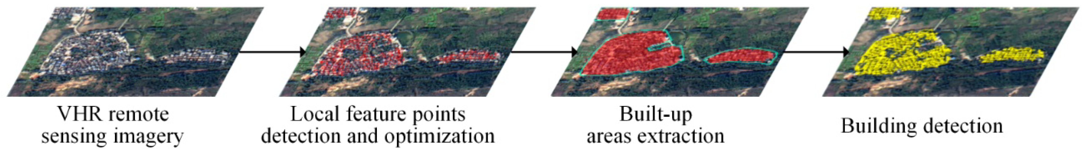
The proposed method is mainly composed of three key steps. First, the local feature points are detected using the Gabor wavelet transform results of the input VHR remote sensing imagery, and then these local feature points are optimized using a proposed saliency index. Next, a spatial voting matrix is computed based on these optimized local feature points to extract built-up areas. Finally, buildings are detected from the built-up areas using the MBI algorithm, and then the initial building detection results are further optimized by the built rule. The flow chart of the proposed method is shown in Figure 1.
2.1. Local Feature Points Detection and Optimization
2.1.1. Local Feature Points Detection
Built-up areas are mainly composed of man-made objects such as buildings and roads. Compared with natural objects, these man-made objects usually produce a large number of local feature points. Since the density of local feature points in built-up areas is higher than that of non-built-up areas, many studies have used the density map of local feature points to identify built-up areas [27,32,33]. In addition, some studies have shown that 2D Gabor wavelets [34] are able to detect salient cues such as local feature points from images. Therefore, we use the Gabor wavelets to extract local feature points.
In order to obtain a complete representation of the image, the input VHR remote sensing image is first decomposed by Gabor wavelets at multi-scales along multi-directions, and then the magnitudes of the decomposition of all scales in each direction are summed up to obtain the Gabor energy map. Given that represents the coordinate of a pixel in the image, represents the scale, represents the direction, and and represent the number of scales and directions, respectively, the Gabor energy map can be defined as
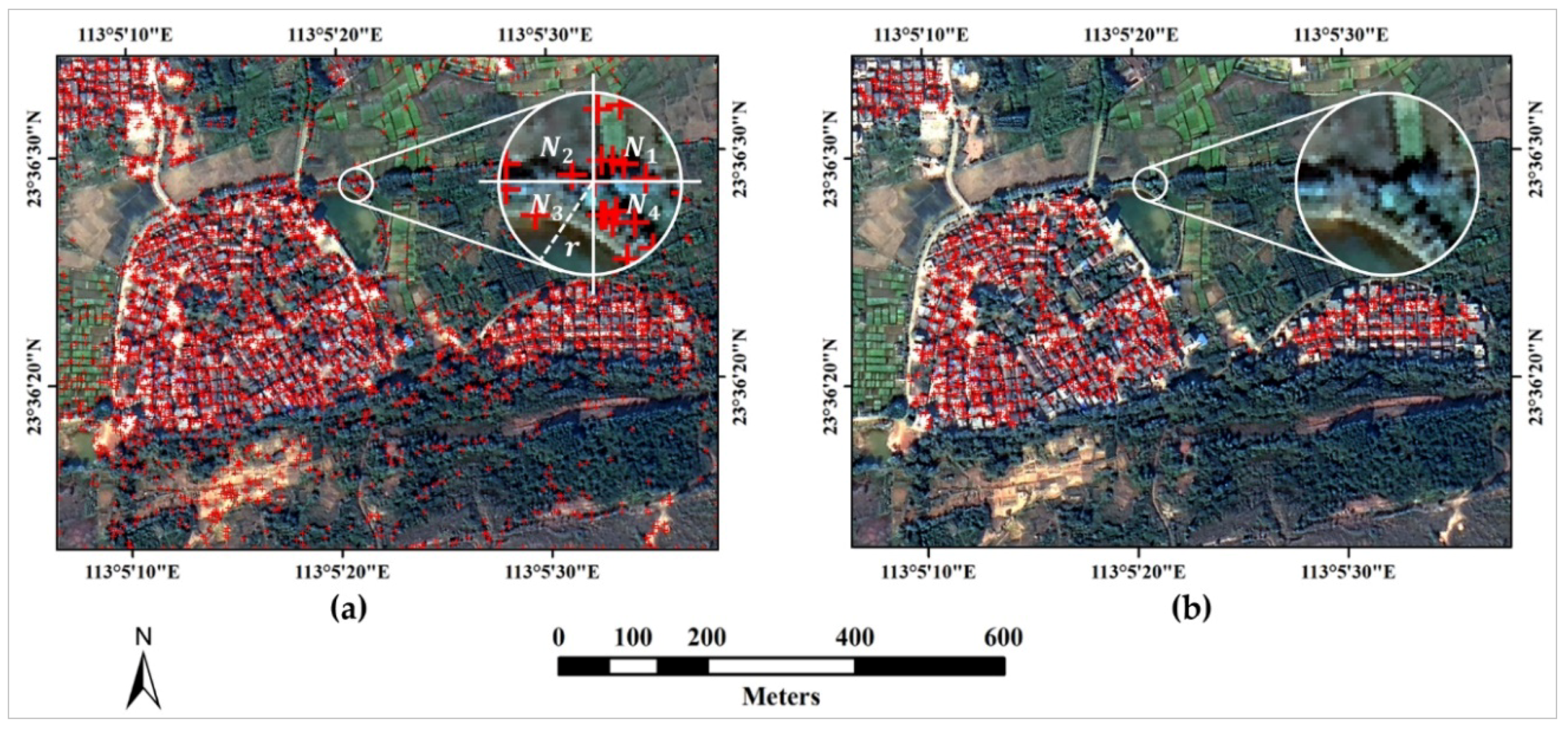
where denotes the magnitude of the decomposition at scale and direction , and denotes the Gabor energy map at direction . After the Gabor energy maps in all directions are obtained, the local feature point detection method proposed by Sirmacek and Unsalan [27] is used to detect local feature points from the Gabor energy maps. More specifically, this method first searches for the local maxima within the eight-connected neighborhoods of all pixels in the Gabor energy map, and these local maxima are taken as candidates for local feature points. Then, these candidate points are optimized according to their magnitude of , and only the candidate whose magnitude is greater than a threshold, which is automatically obtained by performing Otsu’s method on [35], will be retained as the local feature point of direction . Finally, these procedures are applied to the Gabor energy maps in all directions to obtain a local feature point set, noted as . Figure 2a shows an example of using this method to detect local feature points. As shown in Figure 2a, this method not only detects a large number of local feature points in the built-up areas, but also detects many false local feature points in the non-built-up areas. Since these false local feature points will weaken the extraction accuracy of built-up areas, it is necessary to develop a method that can effectively eliminate them.
2.1.2. Local Feature Points Optimization
In order to eliminate these false local feature points located in non-built-up areas and obtain a reliable local feature point set, a saliency index is proposed in this study. The proposal of the saliency index is inspired by the texture saliency index proposed in [36]. These two indices are similar, but their implementation and purpose are completely different. The construction of our proposed saliency index is based on the fact that the local feature points are more densely and evenly distributed in built-up areas than in non-built-up areas. Therefore, we use the density and the distribution evenness of the local feature points in a local circle window to calculate the saliency index. To more clearly describe the derivation process of the saliency index, we use the enlarged circle in Figure 2a as an example for illustration. Given that represents the number of the local feature points in the th quadrant of the local circle window, the spatial distribution evenness parameter can be defined as
where represents the minimum operation, and represents the averaging operation. If there is no local feature point in any of the four quadrants, then is equal to 0, which in turn causes to be equal to 0. In addition, given that represents the radius of the local circle window, represents the number of the local feature points in the local circle window, and represents the number of pixels in the local circle window, the point density parameter can be defined as
where , and . This equation indicates that the more local feature points in the local circle window, the larger the value of . The suggested value of is twice the average size of buildings in the image. For example, the average size of buildings in Figure 2a is about 13 pixels, so the recommended value of is 26 pixels. The sensitivity of built-up areas extraction to the parameter setting will be discussed in Section 4.1.
For each local feature point in , its saliency index can be calculated by the product of and
where the combination of and ensures that only those local feature points that are densely and evenly distributed in the local circle window will have large values. Since the value of the local feature points in built-up areas is higher than that in non-built-up areas, we use the Otsu’ method [35] to automatically calculate the threshold to segment these values to optimize the initial local feature point set , and those local feature points whose values are less than the threshold will be eliminated. Figure 2b shows the result of the optimization of the local feature points using our proposed saliency index. As shown in Figure 2b, those false local feature points located in non-built-up areas are effectively eliminated by our method. More specifically, from the enlarged circle in Figure 2a, we can see that the local feature points located in non-built-up areas are unevenly distributed in the local circle window. The number of the detected local feature points in the first and fourth quadrants of the local circle window is six, and the number of the detected local feature points in the second and third quadrants is two, which causes the calculated value to be relatively low, resulting in a relatively low value. Therefore, we can effectively eliminate these local feature points with low values through threshold processing, as shown in the enlarged circle of Figure 2b. As we obtain the optimized local feature point set, the next step is to use these local feature points to extract built-up areas.
2.2. Built-Up Areas Extraction
Based on the assumption that the probability of existence of built-up areas around the local feature points is high, Sirmacek and Unsalan [27] proposed a spatial voting approach to calculate the voting matrix to measure the probability that each pixel belongs to a built-up area. However, the calculation of the voting matrix is time-consuming. To solve this problem, we adopt the idea of voting based on superpixels in [32] to improve the original voting method, which is achieved by replacing the primary computational unit from pixels to a homogeneous object. In addition, since the cardinality of the optimized local feature point set is so large that using these local feature points to calculate the voting matrix is still time-consuming, we also introduce a local feature point sparse representation method to reduce the cardinality of to further speed up the calculation process. The main steps for extracting built-up areas using the improved method are as follows.
- (1)
- Superpixel segmentation: The simple linear iterative clustering (SLIC) method is used here to partition the input VHR image into superpixels [37]. Given the number parameter and the compactness parameter , the input image will be partitioned into homogeneous objects. In order to automatically handle different images, we set and use the width and height of the input image to calculate the parameter with the expression .
- (2)
- Local feature point sparse representation: This method first searches for the connected components in , and then uses the centroid of the connected component to represent all the local feature points it contains. In this way, the optimized local feature point set can be represented by a sparse local feature point set, noted as , where denotes the centroid coordinate of the th connected component , and denotes the number of connected components. The centroid coordinate of is defined aswhere represents the coordinate of the th local feature point in , and represents the number of the local feature points belonging to .
- (3)
- Calculation of the voting matrix: In order to improve the computational efficiency and extraction accuracy, our improved spatial voting method uses the homogeneous objects as the basic calculation units and combines them with the sparse local feature point set to calculate the voting matrix, which is defined aswhere represents the voting value of the homogeneous object , represents the tolerance parameter of the th connected component , which is calculated by the expression , represents the centroid coordinate of , and represents the centroid coordinate of . Figure 3a shows the voting matrix calculated by the improved spatial voting method. As shown in Figure 3a, the calculated voting matrix can clearly indicate the location of the built-up areas. The high voting value (marked in red) in the voting matrix corresponds to the built-up area, while the low voting value (marked in blue) corresponds to the non-built-up area.
- (4)
- Built-up areas extraction: Since the voting value of the built-up area is higher than that of the non-built-up area, we use the Otsu’ method [35] to segment the voting matrix to extract built-up areas. Figure 3b shows the built-up areas (marked with red-colored area) extracted using the voting matrix shown in Figure 3a. As shown in Figure 3b, the extracted built-up areas match very well with the reference data (marked with cyan-colored polygons), which demonstrates the effectiveness of our improved spatial voting method.
2.3. Building Detection via the MBI Algorithm
The original MBI algorithm [23] is specifically designed for the detection of buildings in urban areas where the density of buildings is high. It fails to detect buildings in rural, agricultural, and mountainous regions. In addition, many irrelevant objects (e.g., open areas, bright barren land, and impervious roads) that have similar spectral characteristics to buildings will generate large numbers of interferences when detecting buildings, and these interferences are difficult to eliminate by conventional methods. In order to solve these problems, we first use the aforementioned method described in Section 2.2 to extract built-up areas from the input image, and then apply the MBI algorithm to detect buildings from the extracted built-up areas.
The calculation of the MBI is briefly described as follows. First, the brightness image, defined by the maximum of all the visible bands, is used as the basic input for building detection. Next, the white top-hat (WTH) transformation of the brightness image is performed in a reconstruction manner to highlight the high local contrast characteristics of buildings, and then the differential morphological profiles (DMP) are constructed based on the multi-scale and multi-directional WTH transformation to represent the complex spatial patterns of buildings in different scales and directions. Since buildings generally exhibit high local contrast and isotropic characteristics, they have larger DMP values than most other objects such as roads in most directions and scales. Therefore, the multi-scale and multi-directional DMP are averaged to calculate the MBI, which is defined as
where and represent the direction and scale of the WTH transformation, and and represent the total number of directions and scales, respectively. Since a large MBI value means that there is a high possibility of the presence of a building structure, we use a preset threshold to binarize the MBI feature image to obtain buildings, where the locations with MBI values greater than will be extracted as buildings. The selection of the value of is based on [23], and a larger value means that more building candidates will be removed.
Detecting buildings from the extracted built-up areas can effectively eliminate most of the interference coming from other irrelevant objects. However, in the initial building detection results, there are still some small errors caused by open areas, vegetation, roads, and small noises. Therefore, to further eliminate these errors, we build a rule based on the shadow, spectral, and geometric information. Given that represents the connected component in the binarization map, the rule is defined as
where denotes the initial building results, denotes the shadow feature map produced by the shadow index proposed in [38], represents the morphological dilation of by a linear structural element in the opposite direction to the solar illumination angle, , , and denote the normalized difference vegetation index, the length–width ratio, and the number of pixels of the connected component, respectively, and , , and represent their corresponding thresholds, respectively. The selection of the values of these thresholds will be discussed in Section 3.2. Since buildings in high-resolution remote sensing images usually cast shadows around them, the rule uses the spatial relationship between buildings and shadows to eliminate false alarms caused by the connected components that are not adjacent to shadows, such as open areas and parking lots. If there is no overlap between and , then will be removed. Furthermore, the rule uses the normalized difference vegetation index to eliminate false alarms caused by the bright vegetation, and it also uses the length–width ratio and the area to eliminate false alarms caused by the elongated and narrow roads and small noises. In this way, our proposed method can not only eliminate the interferences caused by irrelevant objects in non-built-up areas but also remove the false alarms caused by open areas, vegetation, roads, and small noises in built-up areas.
IF IBR(β) ∪ dilate(S(β)) = ∅ OR NDVI(β) > tNDVI OR LWR(β) > tLWR OR Count(β) < tCount,
THEN β should be removed,
THEN β should be removed,
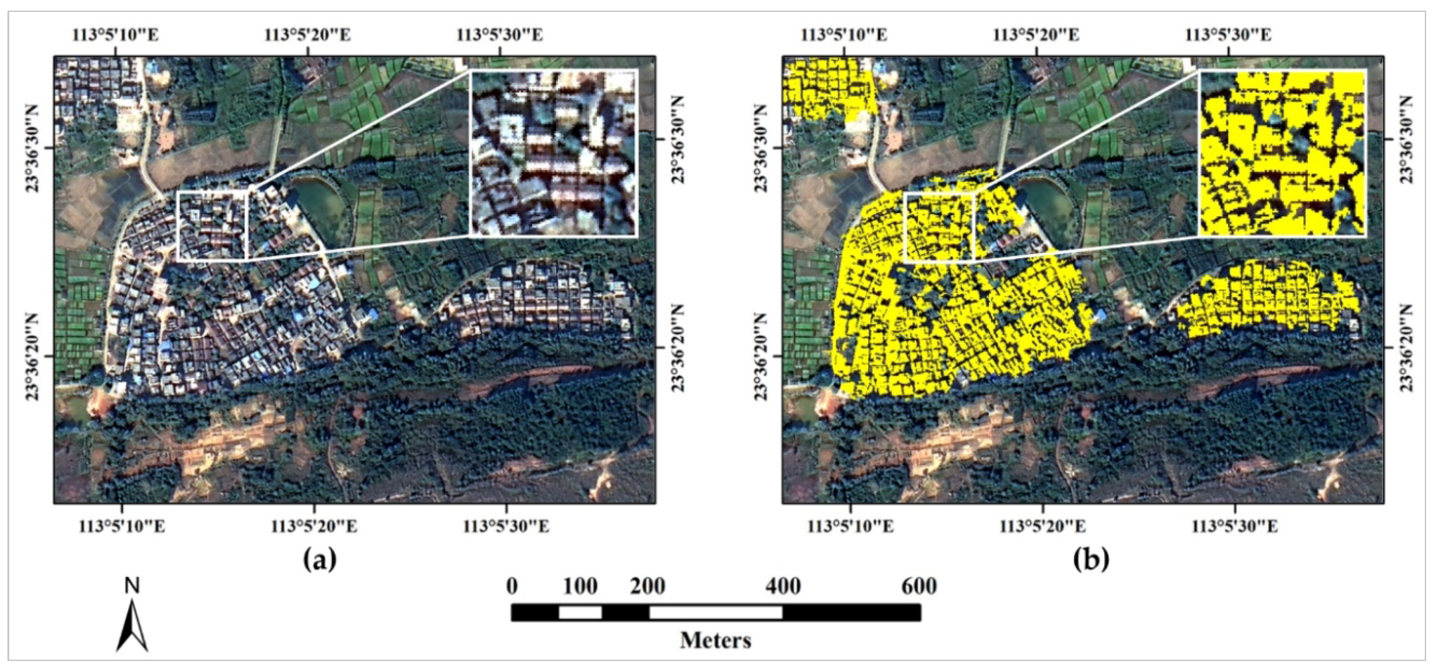
Figure 4a shows the original VHR remote sensing imagery, and Figure 4b shows the building map (marked with yellow-colored areas) detected by our proposed method. As shown in Figure 4b, our method can effectively detect buildings in the image, and it can also eliminate a large amount of interference caused by irrelevant objects that are easily confused with buildings. More specifically, from the enlarged square area shown in Figure 4b, we can see that the detected buildings match very well with the true distribution of the buildings displayed in the enlarged square area in Figure 4a.
3. Experiments
3.1. Data Set Description
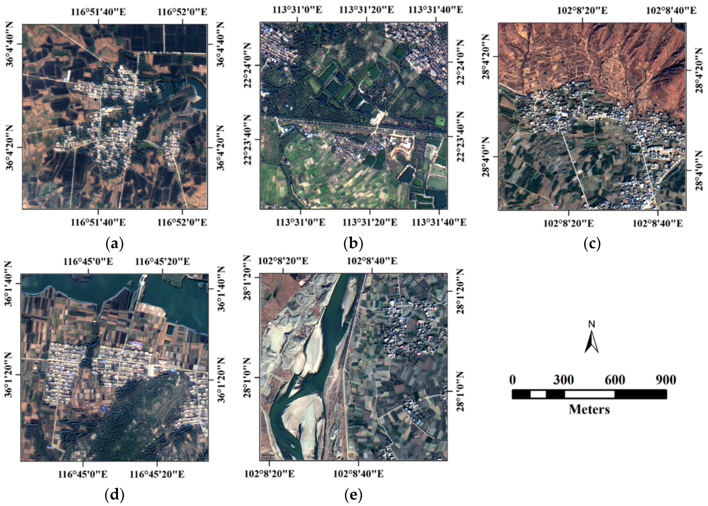
The GaoFen2 satellite is a Chinese high-resolution optical satellite equipped with two panchromatic/multispectral (PAN/MSS) cameras. It was launched on 19 August 2014. The main characteristics of the GaoFen2 satellite are shown in Table 1. In order to evaluate the accuracy of our proposed method, we used five representative image patches selected from three pansharpened GaoFen2 satellite images to perform experiments. The three pansharpened GaoFen2 satellite images are obtained by merging the high spatial resolution panchromatic images with the high spectral resolution multispectral images using the NNDiffuse algorithm [39], and detailed information about them is given in Table 2. As shown in Table 2, the image patches R1 and R4 are selected from the GaoFen2 satellite image with the Scene ID of 3609415; the image patch R2 is selected from the GaoFen2 satellite image with the Scene ID of 3131139, and the image patches R3 and R5 are selected from the GaoFen2 satellite image with the Scene ID of 2097076. All five image patches R1–R5 include four spectral bands (red, green, blue, and near-infrared) with a spatial resolution of 1 m and a size of pixels, and they cover different complex image scenes such as mountainous, agricultural, and rural areas. These image patches are shown in Figure 5. As can be seen from Figure 5, these image patches include a variety of land-cover types such as buildings, impervious roads, bright barren land, mudflats, farmland, vegetation, and water. Among them, impervious roads, bright barren land, and mudflats have similar spectral characteristics to buildings, so they usually cause large numbers of interferences to the detection of buildings. Therefore, using these images for experiments can fully verify the performance of our proposed method. Table 3 shows the number of samples selected for accuracy assessment and the major error sources in each image patch. All the samples were manually labeled by visual interpretation.
3.2. Accuracy Assessment Metrics and Parameter Settings
3.2.1. Accuracy Assessment Metrics
In order to quantitatively evaluate the building detection results, four widely accepted evaluation measures [40] were used in this paper, which are commission error (CE), omission error (OE), overall accuracy (OA), and Kappa coefficient. The CE represents pixels that belong to the background but are labeled as buildings, and the OE represents pixels that belong to a building but are labeled as the background. The OA and the Kappa coefficient are comprehensive indicators for assessing the classification of buildings and backgrounds, which are calculated by the confusion matrix. In addition, since the accurate extraction of built-up areas is a prerequisite for the good performance of our method, we also quantitatively assessed the built-up areas extraction accuracy using the following three metrics: Precision (P), Recall (R), and F-measure (F). Among them, P and R metrics correspond to the correctness and completeness of the built-up areas extraction results, respectively, and F is a comprehensive measure of P and R. The three metrics are defined as
where denotes the number of pixels labeled as built-up area by both reference data and our method, denotes the number of pixels incorrectly labeled as built-up area by our method while they are truly labeled as non-built-up area by reference data, and denotes the number of pixels incorrectly labeled as non-built-up area by our method while they are truly labeled as built-up area by reference data. Meanwhile, a higher F value indicates better performance.
3.2.2. Parameter Settings
Our proposed method mainly involves the following parameters: the parameters , , and for the local feature points detection and optimization, the parameters , , and for the calculation of the MBI, and the parameters , , and for the postprocessing of the building detection results. A detailed description of the selection of these parameters is as follows.
- (1)
- Local feature points detection and optimization parameters: A large number of experiments show that when the scale number and the direction number of the Gabor wavelets are set to 5 and 4, respectively, most of the local feature points in the image can be detected. Therefore, in this study, the values of and are fixed as 5 and 4, respectively. Meanwhile, for the radius of the local circle window, the suggested value is twice the average size of buildings in the image, so it should be tuned according to different test images.
- (2)
- MBI parameters: As analyzed in [23], the four-directional MBI is sufficient to estimate the presence of buildings, and the accuracy of building extraction does not improve significantly as increases. Therefore, in this study, the value of is fixed as 4. For the scale parameter , the suggested value of it is calculated by the expression , where and represent the maximum and minimum sizes of buildings in the image, respectively. Therefore, it needs to be changed according to the test image. For the threshold , its recommended range is [1,6], and a large value will result in a large omission error and a small commission error. This parameter should also be adjusted for different test images.
- (3)
- Postprocessing parameters: For the threshold , according to the author’s experience, its appropriate range is between 0.1 and 0.3, and we can adjust it within this range according to the test images to obtain the best performance. In this study, the parameter is fixed as 0.2. For the thresholds and , since they are relevant to the geometric characteristics of the building, we should also adjust them according to different test images. The appropriate value of should be less than the area of the smallest building in the image to avoid erroneous removal of the building. In this study, the value of is fixed as 20. In addition, after many trials, we determined that the appropriate value of should be greater than 3. In this study, the values of for R1–R5 are 5, 4, 3.5, 4, and 3.5, respectively. Since the postprocessing of the building detection results is to further eliminate some small errors, it does not play a pivotal role in our method. Therefore, these postprocessing parameters (, , and ) are also not critical to our method.
To sum up, the critical parameters of our method are , , , , , and . Among them, the values of , , and are fixed to 5, 4, and 4, respectively, and these values can be used for most images. The parameters that need to be tuned according to different test images are , , and , and their values for the five test images R1–R5 are given in Table 4. The sensitivity of these three parameters will be discussed in Section 4.1.
3.3. Results and Analysis
3.3.1. Built-Up Areas Extraction Results and Analysis
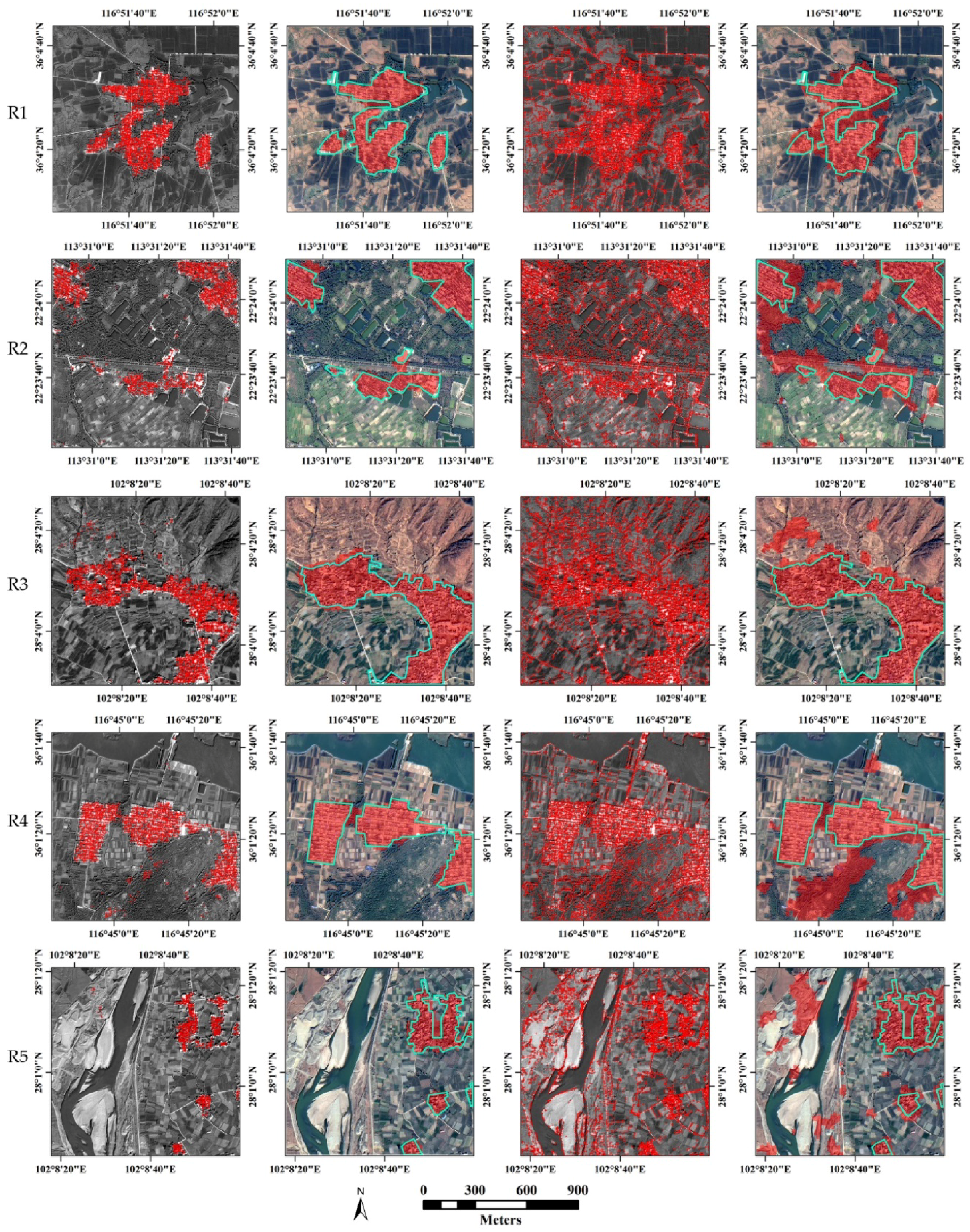
In order to extract built-up areas, images R1–R5 are first decomposed by Gabor wavelets at multi-scales along multi-directions, and then these decomposition results are further processed to obtain local feature points. Next, the proposed saliency index is used to optimize these local feature points. Finally, a voting matrix is calculated based on these optimized local feature points to extract built-up areas. The originally detected local feature points of R1–R5 are shown in the third column of Figure 6, and the results of optimizing these local feature points using the proposed saliency index are shown in the first column of Figure 6. To more clearly display the extraction results of the local feature points, the original VHR remote sensing images are converted into grayscale images for display. From the third column of Figure 6, we can see that a large number of local feature points (marked with red-colored points) are detected over areas with complex textures or salient edges. Among them, many are located in non-built-up areas, which will impair the extraction accuracy of the built-up areas. In contrast, in their optimized results (shown in the first column of Figure 6), there are only a few local feature points in non-built-up areas, which indicates that our proposed saliency index can effectively eliminate the false local feature points located in non-built-up areas and obtain a reliable local feature point set.
The results of the built-up areas extracted using the optimized local feature points are shown in the second column of Figure 6. In addition, to further verify the effectiveness of our proposed saliency index, we also used the originally detected local feature points that were not optimized by the saliency index to extract built-up areas for comparison. The built-up areas extracted using the originally detected local feature points are shown in the fourth column of Figure 6. In the fourth column of Figure 6 we can see that the boundaries of the extracted built-up areas (marked with red-colored area) are very inaccurate, and they incorrectly identify many non-built-up areas as built-up areas. By contrast, as shown in the second column of Figure 6, the built-up areas extracted using the optimized local feature points show very good performance in all test images, which match very well with the reference data (marked with cyan-colored polygons).
The accuracy evaluation results of the built-up areas extracted under these two conditions are provided in Table 5. As shown in Table 5, for the results of the built-up areas extracted using the saliency index, their average precision value is 0.841, their average recall value is 0.936, and their average F-measure value is 0.885, which suggest that our method can effectively extract built-up areas from the image with high correctness and completeness. On the other hand, from Table 5 we can find that the accuracy of the results extracted using the saliency index is better than the accuracy of the results extracted without using the saliency index. Specifically, for each image, the precision value and the F-measure value of the result extracted using the saliency index are higher than that of the result extracted without using the saliency index. For example, when the saliency index is used, the precision value and the F-measure value of R1 are 0.925 and 0.913, respectively, and when the saliency index is not used, the precision value and the F-measure value of R1 are 0.605 and 0.751, respectively. Furthermore, in terms of the average value, the average precision value and the average F-measure value of the results extracted using the saliency index increase by 0.33 and 0.221, respectively, as compared with the results extracted without using the saliency index. The significant improvements of precision and F-measure metrics indicate that our proposed saliency index is very effective in improving the performance of built-up areas extraction. However, it should be noted that the recall value of the results extracted using the saliency index is slightly lower than that of the results extracted without using the saliency index, which is mainly because some small scattered buildings cannot be extracted as built-up areas. According to the above qualitative and quantitative analysis of the built-up areas extraction results, we can prove that our method can accurately extract built-up areas from images by means of the saliency index.
3.3.2. Building Detection Results and Analysis
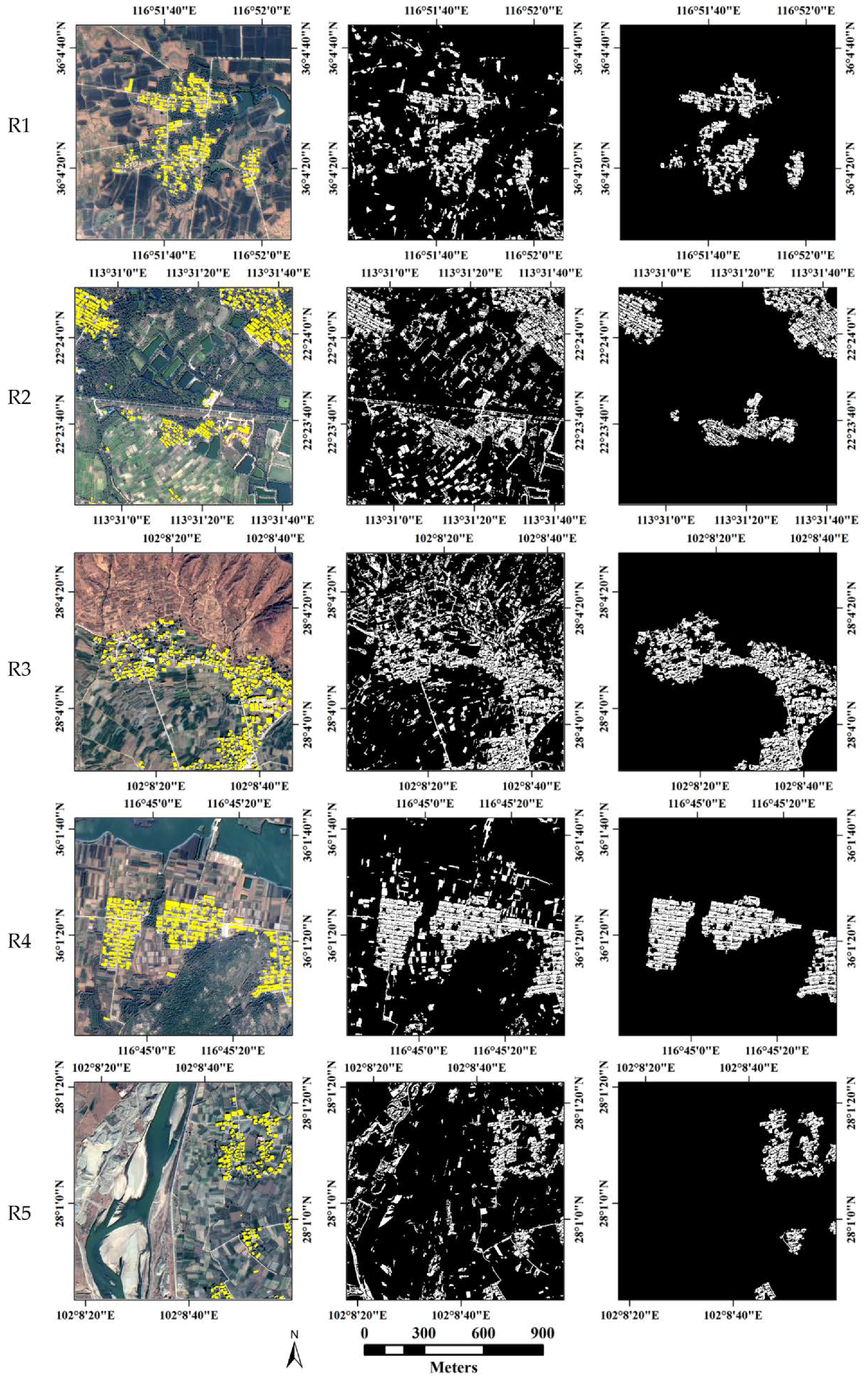
After obtaining the built-up areas of the test images R1–R5, we first use the MBI algorithm to detect buildings from the extracted built-up areas, and then we use the built rule to further eliminate some small errors in the initial building detection results. The final building results of R1–R5 detected by our method are shown in the third column of Figure 7, and their corresponding reference map obtained by visual interpretation (marked with yellow-colored areas) are shown in the first column of Figure 7. In addition, to further verify the effectiveness of our method, we also compared the building detection results of our method with the original MBI algorithm [23]. To ensure the fairness of the comparison, the parameter settings of the original MBI algorithm are consistent with our method. The building results detected by the original MBI algorithm are shown in the second column of Figure 7. As shown in Figure 7, the original MBI algorithm (the second column) performed poorly for all test images as compared with the reference map (the first column). The detected buildings include a large number of irrelevant objects such as farmland, barren land, and impervious roads. In contrast, our method (the third column) can effectively eliminate the interferences from these irrelevant objects and achieve satisfactory results. Taking the test image R5 for illustration, there are several land cover types in the image, including mudflats, bright barren land, impervious roads, buildings, farmland, and river. Among them, bright objects such as mudflats and bright barren land have similar spectral characteristics to buildings and are brighter than their surroundings, which satisfies the brightness hypothesis of the MBI algorithm. Therefore, these bright objects are incorrectly extracted as buildings by the original MBI algorithm. However, our method can eliminate these irrelevant objects and achieve satisfactory performance.
The accuracy evaluation results of building detection are given in Table 6. As depicted in Table 6, the OA of all the test images of our proposed method is greater than 93%, the Kappa coefficient is greater than 0.85, the maximum CE is 11.58%, and the maximum OE is 9.01%. This suggests that our proposed method can effectively distinguish between buildings and backgrounds, and it can also detect buildings with high accuracy and completeness. In addition, from Table 6 we can find that the average CE of the original MBI algorithm is as high as 32%, while our proposed method reduces the average CE to 5.9%, which demonstrates that our proposed method can effectively eliminate large numbers of interferences caused by irrelevant objects. Meanwhile, compared with the original MBI algorithm, the average OA and the average Kappa coefficient of our proposed method increase by 17.55% and 0.342, respectively. The significant improvements of CE, OA, and Kappa coefficient prove that our proposed method remarkably outperforms the original MBI algorithm and can more effectively detect buildings in complex image scenes such as mountainous, agricultural, and rural areas. On the other hand, it should be noted that the OE of our proposed method is slightly larger than the original MBI algorithm, which is mainly because some small scattered buildings have not been recognized during the extraction of built-up areas (first step), so these buildings are not detected in the second step.
4. Discussion
4.1. Parameter Sensitivity Analysis
Our method has three critical parameters (, , and ) that need to be adjusted according to different test images. In this section, we analyzed the effect of the different values of these three parameters on the accuracy of the results.
4.1.1. Sensitivity Analysis of the Parameter
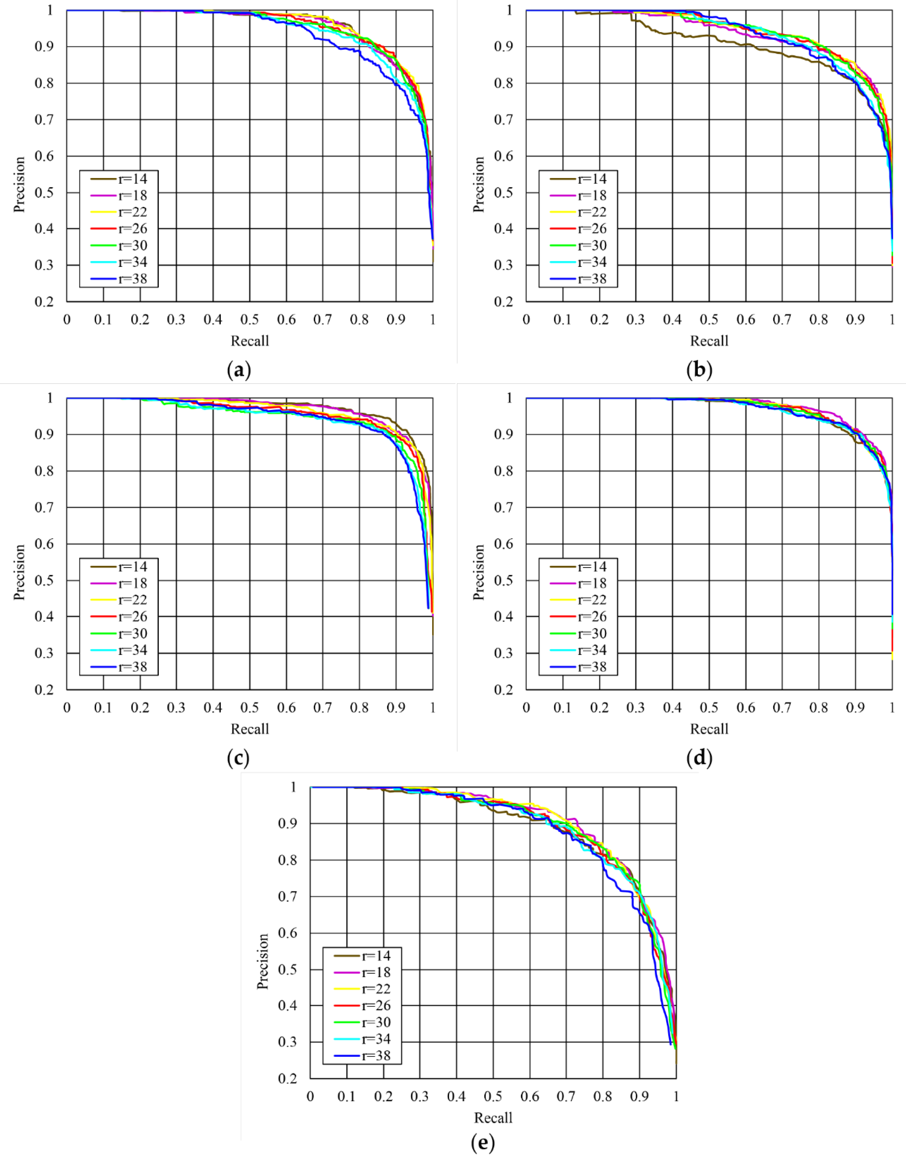
As shown in Figure 2, the proposed saliency index is very effective for the optimization of the local feature point set. It can effectively eliminate a large number of false local feature points located in non-built-up areas, thereby making the extracted built-up areas more accurate. The saliency index contains a tunable parameter, the radius , which is used to control the size of the local circle window. Figure 8 shows the sensitivity of built-up areas extraction to the parameter setting. As depicted in Figure 8, when the value of is about twice the average size of buildings, the corresponding precision–recall curves are very close to each other, which suggests that the extraction of built-up areas is not dramatically sensitive to the value of . In addition, the precision–recall curves also indicate that a good performance can be achieved when the value of is about twice the average size of buildings. Taking the test image R1 for illustration, the average size of buildings in R1 is about 13 pixels. From the precision–recall curves of R1 shown in Figure 8a, we can see that the curve of “r = 26” is close to the curve of “r = 22” and the curve of “r = 30”, and a good performance can be achieved when the value of is close to 26.
4.1.2. Sensitivity Analysis of the Binary Threshold
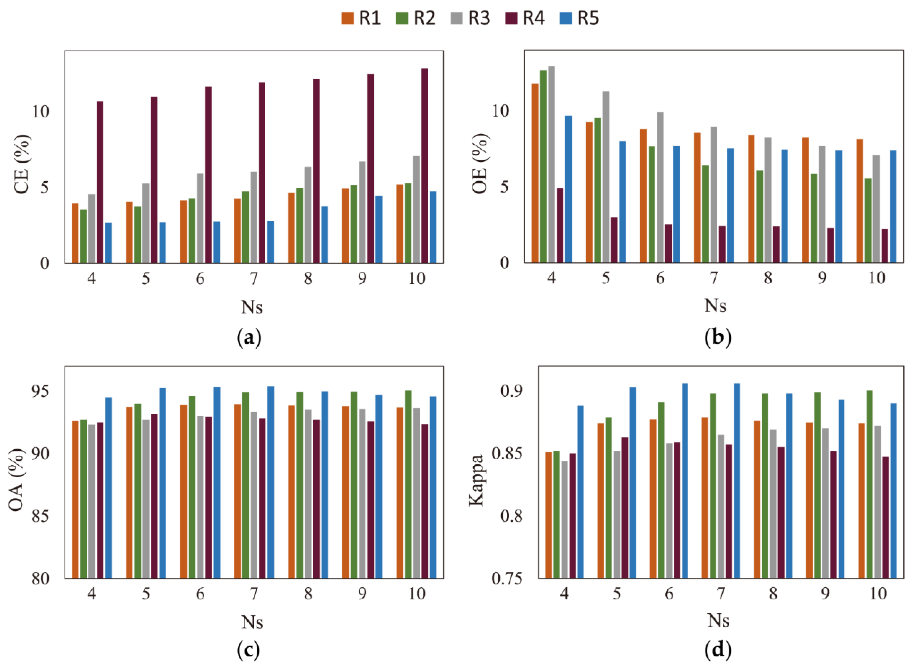
The threshold is used to segment the calculated MBI feature image to obtain buildings. Figure 9 shows the effect of different values on building detection accuracy. As shown in Figure 9, as the threshold increases, the CE of R1–R5 gradually decreases and the OE gradually increases, which suggests that a larger value of will remove more uncertain candidate buildings. At the same time, from Figure 9 we can see that, when the value of is between 1 and 6, the OA and the Kappa coefficient for all test images are very high, and the difference between them is small, but as the value of continues to increase, the OA and the Kappa coefficient begin to decrease, which indicates that the appropriate range of is 1 to 6, and a value of greater than 6 will impair the accuracy of building detection.
4.1.3. Sensitivity Analysis of the Parameter
The parameter is the number of scales of the WTH transformation, which is determined by the size of buildings in the image. The building sizes of R1–R5 range from 4 pixels to 36 pixels, and its corresponding value is 7. Figure 10 shows the effect of different values on building detection accuracy. As shown in Figure 10, as the value of increases, the CE of R1–R5 increases slowly, and the OE decreases slowly, which indicates that a larger value of will extract more buildings. On the other hand, as can be seen from Figure 10, when the value of increases from 4, the OA and the Kappa coefficient of R1–R5 also increase slowly, but when the value of increases to more than 7, the OA and the Kappa begin to decrease slightly, which suggests that the optimal performance can be achieved when the value of is close to the actual size of buildings in the image.
4.2. Merits, Limitations, and Future Work
In this study, we proposed a new building detection method based on the MBI algorithm to detect buildings in complex image scenes. Experiments performed in several representative images demonstrate that the proposed method can effectively detect buildings in VHR remote sensing images and significantly improve on the original MBI algorithm [23]. It achieved good performance with an average OA greater than 93%. In addition, our method has two main advantages. On the one hand, for the detection of buildings, our method can effectively eliminate a large number of false alarms caused by irrelevant objects, which can greatly improve the accuracy of building detection. More specifically, our method first extracts built-up areas from the image and then detects buildings from the extracted built-up areas, which can directly remove a large number of false alarms located in non-built-up areas. Moreover, our method does not rely heavily on the accurate extraction of auxiliary information such as shadows to eliminate false alarms, which is different from most methods. On the other hand, for the extraction of built-up areas, our proposed saliency index solves a common problem in the local feature point extraction, which can greatly improve the extraction accuracy of built-up areas. In addition to these advantages, our method has some limitations that are worth noting.
First, some small scattered buildings cannot be extracted by our method. This is mainly because these small scattered buildings usually produce only a few local feature points, which are easily erroneously eliminated by the saliency index. Therefore, these small scattered buildings cannot be recognized during the extraction of built-up areas (first step), causing them to be missed in the second step. This is also a limitation of our proposed saliency index. In our future work, we will consider incorporating additional information such as short straight lines into the built-up areas extraction process as a supplement to the local feature points to extract these small scattered buildings.
Second, buildings with dark roofs cannot be extracted by our method. Since the MBI algorithm assumes that the building is a bright structure with high local contrast, those buildings with dark roofs will be treated as backgrounds and correspond to low MBI values, which will be removed when binarizing the MBI feature image. In our future work, we will consider combining the spatial features of the building, such as edges, to further judge those areas with relatively low MBI values to avoid erroneous removal.
5. Conclusions
In this paper, we have proposed a new building detection method based on the MBI algorithm to detect buildings from VHR remote sensing images captured in complex environments. This method improves the original MBI algorithm and can effectively detect buildings in non-urban areas. Three key steps are included in our proposed method: local feature points detection and optimization, built-up areas extraction, and building detection. First, the Gabor wavelet transform results of the VHR remote sensing imagery are used to extract local feature points, and then these local feature points are optimized by the proposed saliency index to eliminate the false local feature points located in non-built-up areas. Second, a spatial voting matrix is calculated based on these optimized local feature points to extract built-up areas. Finally, buildings are detected from the extracted built-up areas using the MBI algorithm. Experiments on several representative image patches of GaoFen2 satellite validate the effectiveness of our proposed method for building detection. At the same time, the comparative experiments of built-up areas extraction also proved the effectiveness of our proposed saliency index. In the future, we plan to add additional information to the extraction of built-up areas and the binarization of the MBI feature image to overcome the limitations of our method.
Author Contributions
Y.Y. and S.W. conceived and designed the algorithm and the experiments; Y.M., B.W., G.C., M.S., and W.L. provided help and suggestions in the experiment; G.C. provided help in the paper revision; Y.Y. conducted the experiments and wrote the paper.
Funding
This research was funded by the Strategic Priority Research Program of the Chinese Academy of Sciences: CAS Earth Big Data Science Project (No. XDA19030501), the National Natural Science Foundation of China (Nos. 91547107, 41271426, and 41428103), the Major Program of High Resolution Earth Observation System (No. 30-Y20A37-9003-15/17), and the Science and Technology Research Project of Xinjiang Military.
Acknowledgments
The authors would like to show their gratitude to the editors and the anonymous reviewers for their insightful and valuable comments.
Conflicts of Interest
The authors declare no conflict of interest.
Abbreviations
The abbreviations used in this paper are as follows:
| MBI | morphological building index |
| ISODATA | iterative self-organizing data analysis technique algorithm |
| CNN | convolutional neural network |
| SIFT | scale invariant feature transform |
| DRV | discrimination by ratio of variance |
| SLIC | simple linear iterative clustering |
| WTH | white top-hat |
| DMP | differential morphological profiles |
| IBR | initial building results |
| NDVI | normalized difference vegetation index |
| LWR | length–width ratio |
| CE | commission error |
| OE | omission error |
| OA | overall accuracy |
References
- Ridd, M.K.; Hipple, J.D.; Photogrammetry, A.S.f.; Sensing, R. Remote Sensing of Human Settlements; American Society for Photogrammetry and Remote Sensing: Las Vegas, NV, USA, 2006. [Google Scholar]
- Pesaresi, M.; Guo, H.; Blaes, X.; Ehrlich, D.; Ferri, S.; Gueguen, L.; Halkia, M.; Kauffmann, M.; Kemper, T.; Lu, L. A Global Human Settlement Layer From Optical HR/VHR RS Data: Concept and First Results. IEEE J. Sel. Top. Appl. Earth Obs. Remote Sens. 2013, 6, 2102–2131. [Google Scholar] [CrossRef]
- Florczyk, A.J.; Ferri, S.; Syrris, V.; Kemper, T.; Halkia, M.; Soille, P.; Pesaresi, M. A New European Settlement Map From Optical Remotely Sensed Data. IEEE J. Sel. Top. Appl. Earth Obs. Remote Sens. 2016, 9, 1978–1992. [Google Scholar] [CrossRef]
- Konstantinidis, D.; Stathaki, T.; Argyriou, V.; Grammalidis, N. Building Detection Using Enhanced HOG–LBP Features and Region Refinement Processes. IEEE J. Sel. Top. Appl. Earth Obs. Remote Sens. 2016, 10, 1–18. [Google Scholar] [CrossRef]
- Solano-Correa, Y.T.; Bovolo, F.; Bruzzone, L. An Approach for Unsupervised Change Detection in Multitemporal VHR Images Acquired by Different Multispectral Sensors. Remote Sens. 2018, 10, 533. [Google Scholar] [CrossRef]
- Mayer, H. Automatic object extraction from aerial imagery—A survey focusing on buildings. Comput. Vis. Image Underst. 1999, 74, 138–149. [Google Scholar] [CrossRef]
- Unsalan, C.; Boyer, K.L. A system to detect houses and residential street networks in multispectral satellite images. Comput. Vis. Image Underst. 2005, 98, 423–461. [Google Scholar] [CrossRef]
- Baltsavias, E.P. Object extraction and revision by image analysis using existing geodata and knowledge: Current status and steps towards operational systems. ISPRS-J. Photogramm. Remote Sens. 2004, 58, 129–151. [Google Scholar] [CrossRef]
- Haala, N.; Kada, M. An update on automatic 3D building reconstruction. ISPRS-J. Photogramm. Remote Sens. 2010, 65, 570–580. [Google Scholar] [CrossRef]
- Cheng, G.; Han, J.W. A survey on object detection in optical remote sensing images. ISPRS-J. Photogramm. Remote Sens. 2016, 117, 11–28. [Google Scholar] [CrossRef] [Green Version]
- Lee, D.S.; Shan, J.; Bethel, J.S. Class-guided building extraction from Ikonos imagery. Photogramm. Eng. Remote Sens. 2003, 69, 143–150. [Google Scholar] [CrossRef]
- Inglada, J. Automatic recognition of man-made objects in high resolution optical remote sensing images by SVM classification of geometric image features. ISPRS-J. Photogramm. Remote Sens. 2007, 62, 236–248. [Google Scholar] [CrossRef]
- Senaras, C.; Ozay, M.; Vural, F.T.Y. Building Detection With Decision Fusion. IEEE J. Sel. Top. Appl. Earth Observ. Remote Sens. 2013, 6, 1295–1304. [Google Scholar] [CrossRef]
- Alshehhi, R.; Marpu, P.R.; Woon, W.L.; Dalla Mura, M. Simultaneous extraction of roads and buildings in remote sensing imagery with convolutional neural networks. ISPRS-J. Photogramm. Remote Sens. 2017, 130, 139–149. [Google Scholar] [CrossRef]
- Sirmacek, B.; Unsalan, C. Urban-Area and Building Detection Using SIFT Keypoints and Graph Theory. IEEE Trans. Geosci. Remote Sens. 2009, 47, 1156–1167. [Google Scholar] [CrossRef]
- Ok, A.O.; Senaras, C.; Yuksel, B. Automated Detection of Arbitrarily Shaped Buildings in Complex Environments From Monocular VHR Optical Satellite Imagery. IEEE Trans. Geosci. Remote Sens. 2013, 51, 1701–1717. [Google Scholar] [CrossRef]
- Ok, A.O. Automated detection of buildings from single VHR multispectral images using shadow information and graph cuts. ISPRS-J. Photogramm. Remote Sens. 2013, 86, 21–40. [Google Scholar] [CrossRef]
- Peng, J.; Liu, Y.C. Model and context-driven building extraction in dense urban aerial images. Int. J. Remote Sens. 2005, 26, 1289–1307. [Google Scholar] [CrossRef]
- Ahmadi, S.; Zoej, M.J.V.; Ebadi, H.; Moghaddam, H.A.; Mohammadzadeh, A. Automatic urban building boundary extraction from high resolution aerial images using an innovative model of active contours. Int. J. Appl. Earth Obs. Geoinf. 2010, 12, 150–157. [Google Scholar] [CrossRef]
- Liasis, G.; Stavrou, S. Building extraction in satellite images using active contours and colour features. Int. J. Remote Sens. 2016, 37, 1127–1153. [Google Scholar] [CrossRef]
- Pesaresi, M.; Gerhardinger, A.; Kayitakire, F. A Robust Built-Up Area Presence Index by Anisotropic Rotation-Invariant Textural Measure. IEEE J. Sel. Top. Appl. Earth Obs. Remote Sens. 2008, 1, 180–192. [Google Scholar] [CrossRef]
- Lhomme, S.; He, D.C.; Weber, C.; Morin, D. A new approach to building identification from very-high-spatial-resolution images. Int. J. Remote Sens. 2009, 30, 1341–1354. [Google Scholar] [CrossRef]
- Huang, X.; Zhang, L.P. A Multidirectional and Multiscale Morphological Index for Automatic Building Extraction from Multispectral GeoEye-1 Imagery. Photogramm. Eng. Remote Sens. 2011, 77, 721–732. [Google Scholar] [CrossRef]
- Zhang, Q.; Huang, X.; Zhang, G.X. A Morphological Building Detection Framework for High-Resolution Optical Imagery Over Urban Areas. IEEE Geosci. Remote Sens. Lett. 2016, 13, 1388–1392. [Google Scholar] [CrossRef]
- Huang, X.; Zhang, L. Morphological Building/Shadow Index for Building Extraction From High-Resolution Imagery Over Urban Areas. IEEE J. Sel. Top. Appl. Earth Obs. Remote Sens. 2012, 5, 161–172. [Google Scholar] [CrossRef]
- Huang, X.; Yuan, W.L.; Li, J.Y.; Zhang, L.P. A New Building Extraction Postprocessing Framework for High-Spatial-Resolution Remote-Sensing Imagery. IEEE J. Sel. Top. Appl. Earth Obs. Remote Sens. 2017, 10, 654–668. [Google Scholar] [CrossRef]
- Sirmacek, B.; Unsalan, C. Urban Area Detection Using Local Feature Points and Spatial Voting. IEEE Geosci. Remote Sens. Lett. 2010, 7, 146–150. [Google Scholar] [CrossRef] [Green Version]
- Xu, W.; Huang, X.; Zhang, W. A multi-scale visual salient feature points extraction method based on Gabor wavelets. In Proceedings of the IEEE International Conference on Robotics and Biomimetics, Guilin, China, 19–23 December 2009; pp. 1205–1208. [Google Scholar]
- Kovacs, A.; Sziranyi, T. Improved Harris Feature Point Set for Orientation-Sensitive Urban-Area Detection in Aerial Images. IEEE Geosci. Remote Sens. Lett. 2013, 10, 796–800. [Google Scholar] [CrossRef] [Green Version]
- Hu, Z.; Li, Q.; Zhang, Q.; Wu, G. Representation of Block-Based Image Features in a Multi-Scale Framework for Built-Up Area Detection. Remote Sens. 2016, 8, 155. [Google Scholar] [CrossRef]
- Shi, H.; Chen, L.; Bi, F.K.; Chen, H.; Yu, Y. Accurate Urban Area Detection in Remote Sensing Images. IEEE Geosci. Remote Sens. Lett. 2015, 12, 1948–1952. [Google Scholar] [CrossRef]
- Li, Y.S.; Tan, Y.H.; Deng, J.J.; Wen, Q.; Tian, J.W. Cauchy Graph Embedding Optimization for Built-Up Areas Detection From High-Resolution Remote Sensing Images. IEEE J. Sel. Top. Appl. Earth Obs. Remote Sens. 2015, 8, 2078–2096. [Google Scholar] [CrossRef]
- Tao, C.; Tan, Y.H.; Zou, Z.R.; Tian, J.W. Unsupervised Detection of Built-Up Areas From Multiple High-Resolution Remote Sensing Images. IEEE Geosci. Remote Sens. Lett. 2013, 10, 1300–1304. [Google Scholar] [CrossRef]
- Lee, T.S. Image representation using 2D gabor wavelets. IEEE Trans. Pattern Anal. Mach. Intell. 1996, 18, 959–971. [Google Scholar]
- Otsu, N. A Threshold Selection Method from Gray-Level Histograms. IEEE Trans. Syst. Man Cybern. 1979, 9, 62–66. [Google Scholar] [CrossRef]
- Hu, X.Y.; Shen, J.J.; Shan, J.; Pan, L. Local Edge Distributions for Detection of Salient Structure Textures and Objects. IEEE Geosci. Remote Sens. Lett. 2013, 10, 466–470. [Google Scholar] [CrossRef]
- Achanta, R.; Shaji, A.; Smith, K.; Lucchi, A.; Fua, P.; Susstrunk, S. SLIC Superpixels Compared to State-of-the-Art Superpixel Methods. IEEE Trans. Pattern Anal. Mach. Intell. 2012, 34, 2274–2281. [Google Scholar] [CrossRef] [PubMed]
- Teke, M.; Başeski, E.; Ok, A.Ö.; Yüksel, B.; Şenaras, Ç. Multi-spectral False Color Shadow Detection. In Photogrammetric Image Analysis; Springer: Berlin/Heidelberg, Germany, 2011; pp. 109–119. [Google Scholar]
- Sun, W.; Messinger, D. Nearest-neighbor diffusion-based pan-sharpening algorithm for spectral images. Opt. Eng. 2013, 53, 013107. [Google Scholar] [CrossRef]
- Congalton, R.G.; Green, K. Assessing the Accuracy of Remotely Sensed Data: Principles and Practices; CRC Press: Boca Raton, FL, USA, 2008. [Google Scholar]
Figure 1.
The flow chart of the proposed method.

Figure 2.
Local feature points detection and optimization. (a) Originally detected local feature points; (b) Optimized results by the proposed saliency index.
Figure 2.
Local feature points detection and optimization. (a) Originally detected local feature points; (b) Optimized results by the proposed saliency index.

Figure 3.
Improved spatial voting results. (a) The calculated voting matrix; (b) The extracted built-up areas (marked with red-colored area) and their corresponding reference data (marked with cyan-colored polygons).
Figure 3.
Improved spatial voting results. (a) The calculated voting matrix; (b) The extracted built-up areas (marked with red-colored area) and their corresponding reference data (marked with cyan-colored polygons).

Figure 4.
Building detection results. (a) Original very high resolution (VHR) remote sensing imagery; (b) Building map (marked with yellow-colored areas) detected by our proposed method.
Figure 4.
Building detection results. (a) Original very high resolution (VHR) remote sensing imagery; (b) Building map (marked with yellow-colored areas) detected by our proposed method.

Figure 5.
Five selected test image patches. (a) R1; (b) R2; (c) R3; (d) R4; (e) R5.

Figure 6.
Results of local feature points and built-up areas. (first column) Local feature points (marked with red-colored points) optimized using the proposed saliency index; (second column) The reference data (marked with cyan-colored polygons) and built-up areas (marked with red-colored area) extracted using the optimized local feature points; (third column) Originally detected local feature points (marked with red-colored points); (fourth column) The reference data (marked with cyan-colored polygons) and built-up areas (marked with red-colored area) extracted using the originally detected local feature points.

Figure 7.
Building detection results. (first column) Reference maps of building distribution (marked with yellow-colored areas); (second column) Building maps extracted with the original morphological building index (MBI) algorithm; (third column) Building maps extracted with our method.
Figure 7.
Building detection results. (first column) Reference maps of building distribution (marked with yellow-colored areas); (second column) Building maps extracted with the original morphological building index (MBI) algorithm; (third column) Building maps extracted with our method.

Figure 8.
Built-up areas predication performance under different . (a) The precision–recall curves of R1, where the average size of buildings is 13 pixels; (b) The precision–recall curves of R2, where the average size of buildings is 13 pixels; (c) The precision–recall curves of R3, where the average size of buildings is 12 pixels; (d) The precision–recall curves of R4, where the average size of buildings is 13 pixels; (e) The precision–recall curves of R5, where the average size of buildings is 12 pixels.

Figure 9.
Building detection accuracy under different values of . (a) commission error (CE); (b) omission error (OE); (c) overall accuracy (OA); (d) Kappa coefficient.
Figure 9.
Building detection accuracy under different values of . (a) commission error (CE); (b) omission error (OE); (c) overall accuracy (OA); (d) Kappa coefficient.

Figure 10.
Building detection accuracy under different values of . (a) CE; (b) OE; (c) OA; (d) Kappa coefficient.
Figure 10.
Building detection accuracy under different values of . (a) CE; (b) OE; (c) OA; (d) Kappa coefficient.


Table 1.
The main characteristics of the GaoFen2 satellite.
| Sensor Specification | Panchromatic | Multispectral |
|---|---|---|
| Spatial Resolution | 1 m | 4 m |
| Swath Width | 45 km | 45 km |
| Repetition Cycle | 5 days | 5 days |
| Spectral Range | 450~900 nm | Blue: 450~520 nm Green: 520~590 nm Red: 630~690 nm Near-infrared: 770~890 nm |
Table 2.
The GaoFen2 satellite images used for the detection of buildings in this study.
| Scene ID | Acquisition Date and Time (UTC) | Image Locations | Image Patches |
|---|---|---|---|
| 3609415 | 30 April 2017, 11:27:58 | Tai’an City, China | R1, R4 |
| 3131139 | 18 December 2016, 11:31:01 | Zhongshan City, China | R2 |
| 2097076 | 14 February 2016, 12:11:49 | Xichang City, China | R3, R5 |
Table 3.
Number of samples and major error sources for R1–R5.
| Image | Number of Samples | Major Error Sources | |
|---|---|---|---|
| Building | Background 1 | ||
| R1 | 11218 | 11814 | bright barren land, impervious roads |
| R2 | 12989 | 14816 | impervious roads, open areas, farmland |
| R3 | 10334 | 12115 | bright barren land, impervious roads, farmland |
| R4 | 11028 | 12395 | bright barren land, impervious roads, farmland |
| R5 | 7120 | 7986 | bright barren land, farmland, mudflats |
1 Background refers to the area that is not a building.
Table 4.
Critical parameter settings of our method.
| Image | |||
|---|---|---|---|
| R1 | 26 | 7 | 4 |
| R2 | 26 | 7 | 5 |
| R3 | 24 | 7 | 5 |
| R4 | 26 | 7 | 4 |
| R5 | 24 | 7 | 5 |
Table 5.
The accuracy evaluation results of built-up areas extraction.
| Image | With the Saliency Index 1 | Without the Saliency Index 2 | ||||
|---|---|---|---|---|---|---|
| Precision | Recall | F-Measure | Precision | Recall | F-Measure | |
| R1 | 0.925 | 0.901 | 0.913 | 0.605 | 0.989 | 0.751 |
| R2 | 0.812 | 0.930 | 0.867 | 0.435 | 0.998 | 0.606 |
| R3 | 0.849 | 0.978 | 0.909 | 0.720 | 0.996 | 0.836 |
| R4 | 0.857 | 0.940 | 0.896 | 0.458 | 0.998 | 0.628 |
| R5 | 0.762 | 0.931 | 0.838 | 0.335 | 0.993 | 0.501 |
| Average | 0.841 | 0.936 | 0.885 | 0.511 | 0.995 | 0.664 |
1 The results of the built-up areas extracted using the saliency index. 2 The results of the built-up areas extracted without using the saliency index.
Table 6.
Accuracy assessment of building detection for the original MBI algorithm and our method.
| Image | Accuracy Assessment | |||||||
|---|---|---|---|---|---|---|---|---|
| The Original MBI Algorithm | Our Proposed Method | |||||||
| CE (%) | OE (%) | OA (%) | Kappa | CE (%) | OE (%) | OA (%) | Kappa | |
| R1 | 28.82 | 7.50 | 78.11 | 0.565 | 4.33 | 8.60 | 93.79 | 0.876 |
| R2 | 32.02 | 3.96 | 77.02 | 0.549 | 4.58 | 6.57 | 94.84 | 0.896 |
| R3 | 37.86 | 8.30 | 70.46 | 0.426 | 6.29 | 9.01 | 93.05 | 0.860 |
| R4 | 32.92 | 1.92 | 76.43 | 0.539 | 11.58 | 2.36 | 92.87 | 0.858 |
| R5 | 28.64 | 3.48 | 80.10 | 0.608 | 2.74 | 7.36 | 95.29 | 0.905 |
| Average | 32.05 | 5.03 | 76.42 | 0.537 | 5.90 | 6.78 | 93.97 | 0.879 |
© 2018 by the authors. Licensee MDPI, Basel, Switzerland. This article is an open access article distributed under the terms and conditions of the Creative Commons Attribution (CC BY) license (http://creativecommons.org/licenses/by/4.0/).
Share and Cite
MDPI and ACS Style
You, Y.; Wang, S.; Ma, Y.; Chen, G.; Wang, B.; Shen, M.; Liu, W. Building Detection from VHR Remote Sensing Imagery Based on the Morphological Building Index. Remote Sens. 2018, 10, 1287. https://doi.org/10.3390/rs10081287
AMA Style
You Y, Wang S, Ma Y, Chen G, Wang B, Shen M, Liu W. Building Detection from VHR Remote Sensing Imagery Based on the Morphological Building Index. Remote Sensing. 2018; 10(8):1287. https://doi.org/10.3390/rs10081287
Chicago/Turabian StyleYou, Yongfa, Siyuan Wang, Yuanxu Ma, Guangsheng Chen, Bin Wang, Ming Shen, and Weihua Liu. 2018. "Building Detection from VHR Remote Sensing Imagery Based on the Morphological Building Index" Remote Sensing 10, no. 8: 1287. https://doi.org/10.3390/rs10081287
Note that from the first issue of 2016, this journal uses article numbers instead of page numbers. See further details here.