Assessing Coastal SMAP Surface Salinity Accuracy and Its Application to Monitoring Gulf of Maine Circulation Dynamics


1
Department of Atmospheric and Oceanic Science, University of Maryland, College Park, MD 20742, USA
2
Ocean Process Analysis Laboratory, Institute for the Study of Earth, Oceans, and Space, University of New Hampshire, Durham, NH 03824, USA
*
Author to whom correspondence should be addressed.
Remote Sens. 2018, 10(8), 1232; https://doi.org/10.3390/rs10081232
Submission received: 22 June 2018
/
Revised: 1 August 2018
/
Accepted: 3 August 2018
/
Published: 6 August 2018
(This article belongs to the Special Issue Sea Surface Salinity Remote Sensing)
Abstract
:Monitoring the cold and productive waters of the Gulf of Maine and their interactions with the nearby northwestern (NW) Atlantic shelf is important but challenging. Although remotely sensed sea surface temperature (SST), ocean color, and sea level have become routine, much of the water exchange physics is reflected in salinity fields. The recent invention of satellite salinity sensors, including the Soil Moisture Active Passive (SMAP) radiometer, opens new prospects in regional shelf studies. However, local sea surface salinity (SSS) retrieval is challenging due to both cold SST limiting salinity sensor sensitivity and proximity to land. For the NW Atlantic, our analysis shows that SMAP SSS is subject to an SST-dependent bias that is negative and amplifies in winter and early spring due to the SST-related drop in SMAP sensor sensitivity. On top of that, SMAP SSS is subject to a land contamination bias. The latter bias becomes noticeable and negative when the antenna land contamination factor (LC) exceeds 0.2%, and attains maximum negative values at LC = 0.4%. Coastward of LC = 0.5%, a significant positive land contamination bias in absolute SMAP SSS is evident. SST and land contamination bias components are seasonally dependent due to seasonal changes in SST/winds and terrestrial microwave properties. Fortunately, it is shown that SSS anomalies computed relative to a satellite SSS climatology can effectively remove such seasonal biases along with the real seasonal cycle. SMAP monthly SSS anomalies have sufficient accuracy and applicability to extend nearer to the coasts. They are used to examine the Gulf of Maine water inflow, which displayed important water intrusions in between Georges Banks and Nova Scotia in the winters of 2016/17 and 2017/18. Water intrusion patterns observed by SMAP are generally consistent with independent measurements from the European Soil Moisture Ocean Salinity (SMOS) mission. Circulation dynamics related to the 2016/2017 period and enhanced wind-driven Scotian Shelf transport into the Gulf of Maine are discussed.
1. Introduction
Monitoring interactions between the cold and productive waters of the Gulf of Maine (GoM) and the adjoining northwestern Atlantic shelf is an important yet challenging regional need, with seasonal and longer timescale change impacts that affect ecosystem, fishery, and coastal management efforts. Key water mass inflows influencing this marginal sea include the upstream fresh/cold Scotian Shelf and Labrador Sea currents, and the adjoining salty/warm northwestern (NW) Atlantic shelf (Mountain [1]; Townsend et al. [2]; Feng et al. [3]; Peterson et al. [4]). The primary inflow to the GoM is through deep, typically salty, water along the Northeast Channel (NEC) that lies between Browns and Georges Banks (see Figure 1). Separately, fresher Scotian Shelf water enters through the relatively shallow (100 m) Northern Channel between Cape Sable and Browns Bank (Ramp et al. [5]; Feng et al. [3]). The variability and relative strength of these transports are thought to control interior Gulf of Maine nutrient and density levels (Townsend et al. [2]).
The dominance of subsurface GoM exchange pathways has, so far, limited the utility of surface remote sensing data for monitoring GoM dynamics. However, Feng et al. [3] recently used altimeter data to demonstrate that seasonal and interannual variability in near-surface freshwater advection from the Scotian Shelf into the coastal GoM can be related to local wind-induced changes in the remote upstream coastal geostrophic currents. That study, amongst others cited, highlighted the need to resolve spatial information on surface salinity fields just offshore of and inside the GoM. While focused on open ocean waters, two recent NW Atlantic sea surface salinity (SSS) studies showed new satellite capabilities to resolve along shelf dynamics and Gulf Stream perturbations (Grodsky et al. [6] and Reul et al. [7]). The present study explores SSS data capabilities nearer to shore and in colder waters, including a focus on wintertime interactions between the GoM and NW Atlantic shelf slope region. For this, we use Soil Moisture Active Passive (SMAP) microwave SSS data at a spatial resolution near 40 km. This is a courser resolution than that used for visible or infrared sea surface temperature (SST) data (1–10 km), but it provides weekly-to-monthly data that is unaffected by winter period rain and clouds. The choice of microwave remote sensing data is important, because stronger NEC transport events into the GoM tend to occur in winter (Ramp et al. [5]) when SST is cold and its gradients are at their weakest due to strong surface cooling.
The application of microwave data for SSS observation in marginal seas is complicated by proximity to land (e.g., Dinnat and LeVine [8]). A few successful applications of satellite SSS to study salinity variation near to shore have been in warmer tropical seas where the measurement sensitivity is higher (e.g., Gierach et al. [9]). However, salinity retrievals over cold coastal seas must contend with both known major and competing sources of bias, water temperature, and land effects. Satellite SSS is subject to an SST-dependent bias that is, at present, negative and amplified in winter and early spring due to the SST-related drop in microwave sensor sensitivity (e.g., Köhler et al. [10]; Meissner et al. [11]). On top of that, satellite SSS is subject to a land contamination bias (e.g., Tang et al. [12]). The two bias components have pronounced seasonal signatures due to seasonal changes in SST-related sensor sensitivity and land emissivity. Global ocean SSS analyses have shown that if one is interested in true SSS change (e.g., seasonal anomalies) with respect to these consistently repeating biases, then one can reference SSS data to the sensor-specific SSS climatology to obtain the anomaly. This effectively removes or strongly attenuates all such bias effects. Thus, we expect that the monthly SSS anomalies used for dynamical analyses in this paper have sufficient accuracy and applicability to extend beyond the tropics to mid-latitude oceans and nearer to the coast (Boutin et al. [13]; Lee [14]). This expectation is aided by the relatively large, ~1 psu, spatial and temporal salinity changes that are often observed across the NW Atlantic shelf, which are gradients that are known to be detectable by remote sensing salinity (e.g., Kubryakov et al. [15]; Garcia-Eidell et al. [16]).
In this paper, we first address SMAP SSS data accuracy using concurrent buoy, Array for Real-Time Geostrophic Oceanography (Argo) float, glider, and thermosalinograph datasets with a focus on the land contamination (LC) and SST biases. We also seek to demonstrate that one can successfully remove the observed seasonal SSS cycle to retrieve an accurate estimate of the monthly SMAP SSS anomaly across this marginal sea region. We then compare apparent water mass changes within the GoM and between Georges Banks and the Scotian Shelf in the winters of 2016/17 and 2017/18. Regional wind speed data suggest that the 2016/17 GoM freshening event is likely tied to enhanced Scotian Shelf water inflow in fall 2016.
2. Materials and Methods
Satellite SSS: SMAP SSS data are provided globally and daily using an eight-day running mean on a 0.25o spatial grid (Version 2 as produced by the Remote Sensing Systems (RSS, www.remss.com/missions/smap, Meissner and Wentz [17]) with the effective spatial resolution of ~40 km. Besides SSS retrieval, this dataset provides reference sea surface temperature (SST) as well as antenna land contamination (LC or GLAND) and ice contamination (GICE) fractions (both weighted by antenna gain). To independently confirm and support SMAP results, we also use the debiased 0.25° SSS dataset obtained using the European Soil Moisture Ocean Salinity sensor (SMOS version 2.0, www.catds.fr/sipad/; Boutin et al. [18]).
Mooring data: As noted earlier, satellite SSS data in colder waters (<5–7 °C) and approaching coastlines are still subject to several limitations that may lead to regional and seasonally dependent SSS biases (e.g., Meissner et al. [11]). Fortunately, a number of observational programs are providing valuable salinity ground truth measurements to aid in the characterization of measurement noise and bias. The NorthEastern Regional Association of Coastal and Ocean Observing Systems (NERACOOS) operates a number of GoM coastal and deeper basin moorings (gyre.umeoce.maine.edu/buoyhome.php). We focus on the mid-basin GoM mooring (M01, 2003-present, Figure 1) located in Jordan Basin and the most seaward mooring located in the Northeast Channel (NEC) to monitor GoM inflows (N01, 2004–2017, Figure 1). These buoys monitor temperature and salinity (S), including measurements at depths of 1 m, 20 m, and 50 m. A more recent addition (2014–present) to this regional observation system is provided by the Ocean Observing Initiative (OOI, https://ooinet.oceanobservatories.org/). Their coastal PIONEER array includes an offshore surface mooring (ASIMET Bulk Meteorology Instrument Package) that monitors 1-m depth salinity. Daily buoy S anomalies at each buoy were computed by calculating monthly seasonal cycles (based on the full buoy data temporal coverage) and daily resampling using cubic spline interpolation. All of the buoy data have been averaged daily, in part to reduce the significant variability associated with tides.
Thermosalinograph and glider: Another valuable data source that was used here specifically for SMAP SSS land contamination assessment is ship-based thermosalinograph (TSG) observations collected near coastlines. Study data come from the long-term M/V Oleander transect program (http://po.msrc.sunysb.edu/Oleander). These along transect salinity measurements (3-m depth) cover from the (United States) US east coast to Bermuda with near monthly sampling. Salinity data quality was confirmed against Argo float datasets from 2012–2016. We also use a second higher-latitude Atlantic TSG dataset collected by the M/V NUKA-ARCTICA, which are data that are quality controlled, flagged, and distributed by the Laboratoire d’Etudes en Géophysique et Océanographie (LEGOS) (www.legos.obs-mip.fr/observations/sss/datadelivery/dmdata/). These data include Europe–Greenland transects and episodic summer period coastal Labrador Sea and Greenland coastline visits. Only NUKA-ARCTICA salinity observations that have been flagged as good are used. In the RSS SMAP v.2.0 gridded product, SSS is set to an undefined value for sea ice concentration, GICE > 0.1%. There are no valid SMAP/TSG collocations for GICE > 0.1%. Even after this ice-filtering criterion, GICE > 0.1, some residual sea-ice contamination could still persist. Their possible remaining effect on the SMAP/TSG matchups is not considered herein, but may lead to a fresh SMAP SSS bias (see Section 3.2, Tang et al. [19]). For additional in situ context, Slocum glider T/S data (near-surface data are from 3–5 m) on the Scotian Shelf in fall 2016 and 2017 were obtained via the Marine Environmental Observation Prediction and Response Network (MEOPAR) at gliders.oceantrack.org/data/slocum. Glider near-surface salinity data are averaged across a given day to provide one daily estimate at a daily center position.
Argo data: Our chosen global near-surface in situ salinity database uses the daily 1° × 1° binned version of the original Argo profiles, which are available from ftp://usgodae.org/. The shallowest depth Argo level (typically 5–10 m) is used as a proxy for SSS.
Other satellite data: Finally, the AVISO multi-satellite merged absolute dynamic topography and its related geostrophic currents are used to identify regional ocean circulation dynamics. These satellite altimeter data products are now distributed through the Copernicus Marine Environment Monitoring Service (http://marine.copernicus.eu). Gridded 10-m near-surface winds from the Advanced Scatterometer (ASCAT) scatterometer onboard the European Meteorological Satellite Organization MetOp (ftp.ifremer.fr/ifremer/cersat/products/gridded/MWF/L3/ASCAT) are produced by Bentamy and Croize-Fillon [20].
All of the anomalies used in this paper are calculated as deviations from corresponding monthly seasonal cycles.
3. Results
3.1. SMAP SSS Bias Characterization
3.1.1. Global Distribution of SMAP Bias from Comparisons with Argo
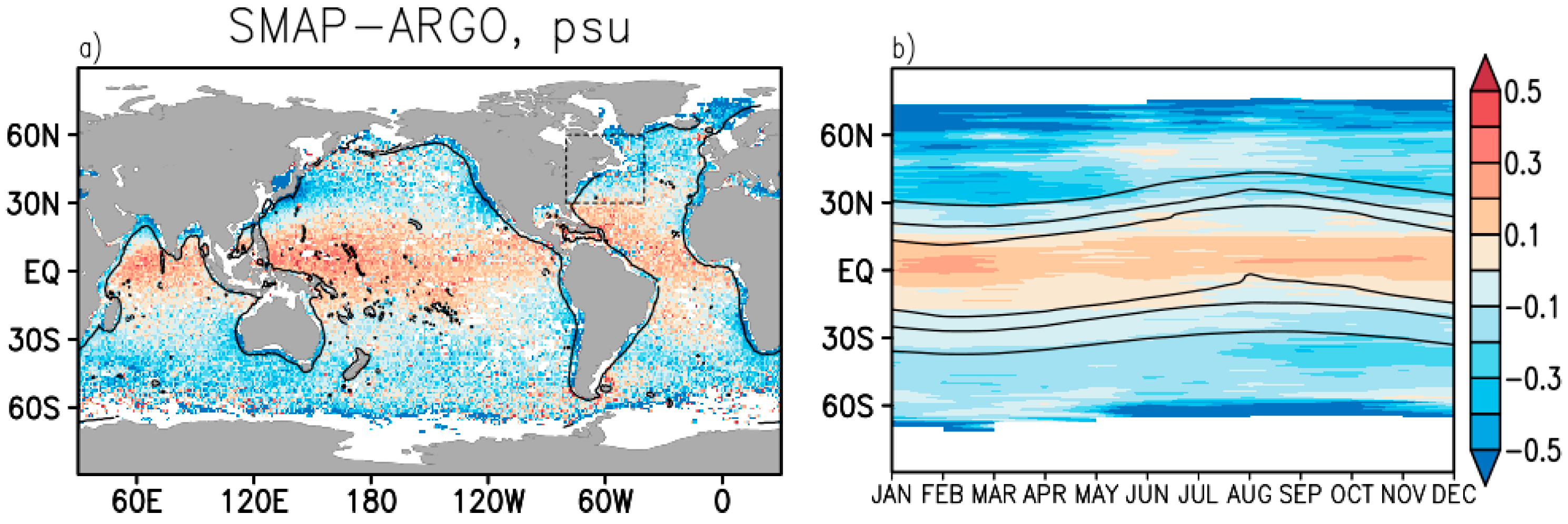
The general characterization of SMAP versus in situ salinity differences (bias hereafter) is illustrated by comparison to quasi-synchronous (same day) Argo salinity measurements, as shown in Figure 2. The time mean SMAP bias (Figure 2a) has a clear spatial distribution (resembling SST, Melnichenko personal communication) with a salty bias in the warmer tropics and a fresh bias in the colder mid-latitude ocean. Noting the strong seasonal cycle of SST, one may anticipate a corresponding seasonal variation in the bias. This time variability is indeed present, but mostly for the higher latitude fresh bias regions where the magnitude increases during cold seasons (Figure 2b). In contrast, the tropical positive bias has only minor seasonal changes, in turn suggesting it may not be related to SST (Tang et al. [12]). Also, note these bias estimates implicitly include any haline stratification that is present between the surface and the shallowest Argo measurement level ~5 m, which is a factor that at present is poorly characterized (Grodsky et al. [21]; Liu et al. [22]; Song et al. [23]).
Besides the meridional structure, the SMAP SSS biases in Figure 2a also depict clear negative patterns in coastal areas. This fresh along coast bias feature is present at all latitudes, including the tropics, reflecting an underestimation of salinity due to the SMAP antenna land contamination (LC, leakage of land surface radiation through antenna side lobes). These coastal features have significant impacts on the accuracy of SMAP SSS over the northwestern (NW) Atlantic shelf, which is our area of focus. Most of the NW shelf shows a negative SSS bias (Figure 1a) that can be examined with further coastal and independent in situ measurements.
3.1.2. SMAP Comparison with TSG Data
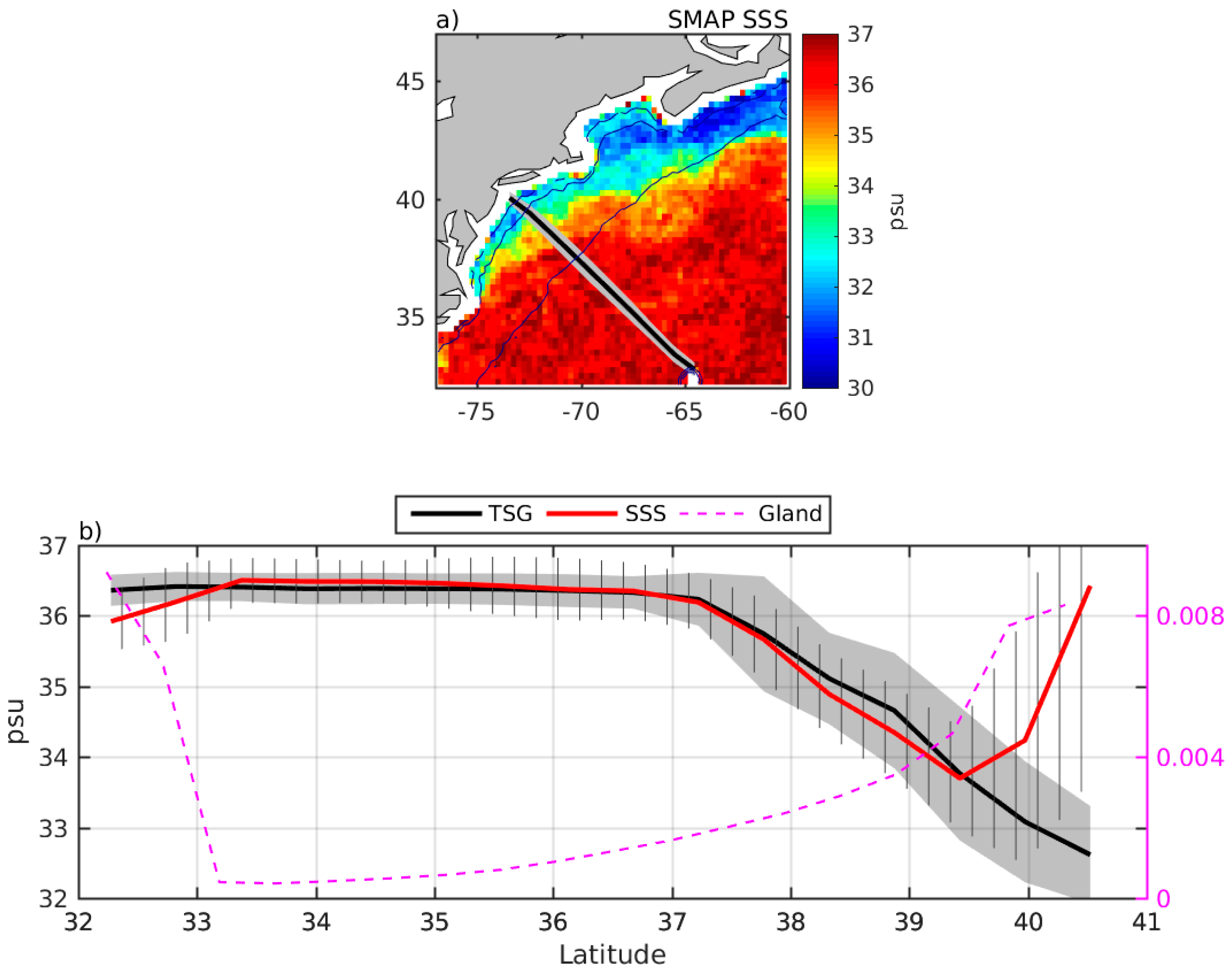
Figure 3 data indicate that the Oleander TSG salinity data are remarkably consistent with collocated (same day, 25-km search radius) SMAP SSS over the open ocean south of the Gulf Stream (latitude, or LAT < 37°N). This consistency partly contradicts the fresh bias versus Argo salinity (Figure 2a), which is a point to be addressed later. The negative SMAP bias becomes noticeable only approaching the continent (LAT > 37.5°N) as well as approaching Bermuda (LAT < 33.5°N). There is also a large salty bias very close to the continent (for , LAT > 39.5°N), which may be interpreted as a result of an overestimation of the land contamination impact. Note that coastal areas, where SMAP land contamination levels likely require attention, cover much of the GoM (Figure 3a).
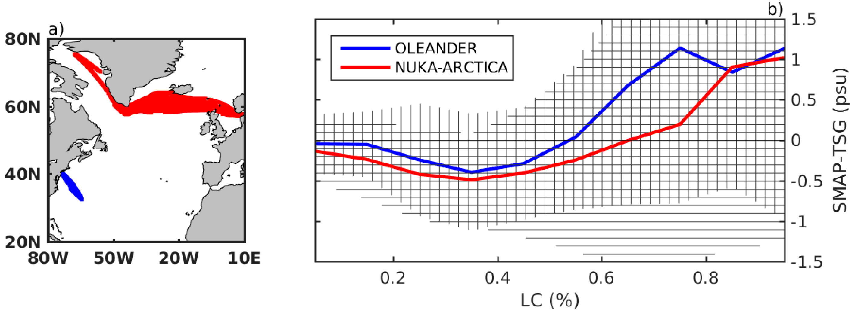
Conditionally, the total SMAP bias can be partitioned into two major components. We define an inherent SMAP retrieval bias (SRB) as being the SSS bias for open ocean conditions; i.e., away from coastal impacts. A second land contamination bias (LCB) is solely due to land-based emissivity that enters through the side lobes of SMAP antenna. Binning SMAP-TSG S differences versus LC reveals that time mean LCB becomes noticeable in the M/V OLEANDER dataset at , and reaches maximum negative values at (Figure 4). Closer to the coast (), the LCB switches to positive values due to an overestimation of the LC effect. Although this behavior should be geographically dependent due to relative changes in sea and land microwave properties, it is generally confirmed by the separate TSG data from the M/V NUKA-ARCTICA collected in the colder North Atlantic region (Figure 4). The SMAP biases along these more northern NUKA-ARCTICA transects have slightly larger negative values than SMAP biases along OLEANDER transects, perhaps due to the contribution from the time mean SRB, which is more negative over cold SST.
We predict that both SRB and LCB will be seasonally dependent due to seasonal changes in ocean conditions (SST, wind) and in terrestrial microwave properties (soil moisture, in particular), respectively. The more extensive Oleander transect time coverage allows the best TSG-based seasonal characterization of SMAP bias, but only locally along the mean transect line (Figure 5). Note that the Figure 5 endpoint data also need to consider varying distance to nearby land (hence the LC factor, see also Figure 3a). Close to Bermuda (LAT 33°N) and approaching the continent (37°N LAT 39.5°N), the bias is mostly negative due to land contamination and has stronger negative values in colder seasons. In line with Figure 3b, the LCB becomes positive (>1 psu) closer to the coast (LAT 39.5°N), reflecting an overestimation of the LC effect. This overestimation has clear seasonal dependence. It is weaker or even reversed in boreal fall. This may reflect uncorrected seasonal changes in sea–land temperature contrasts and land emissivity (moisture).
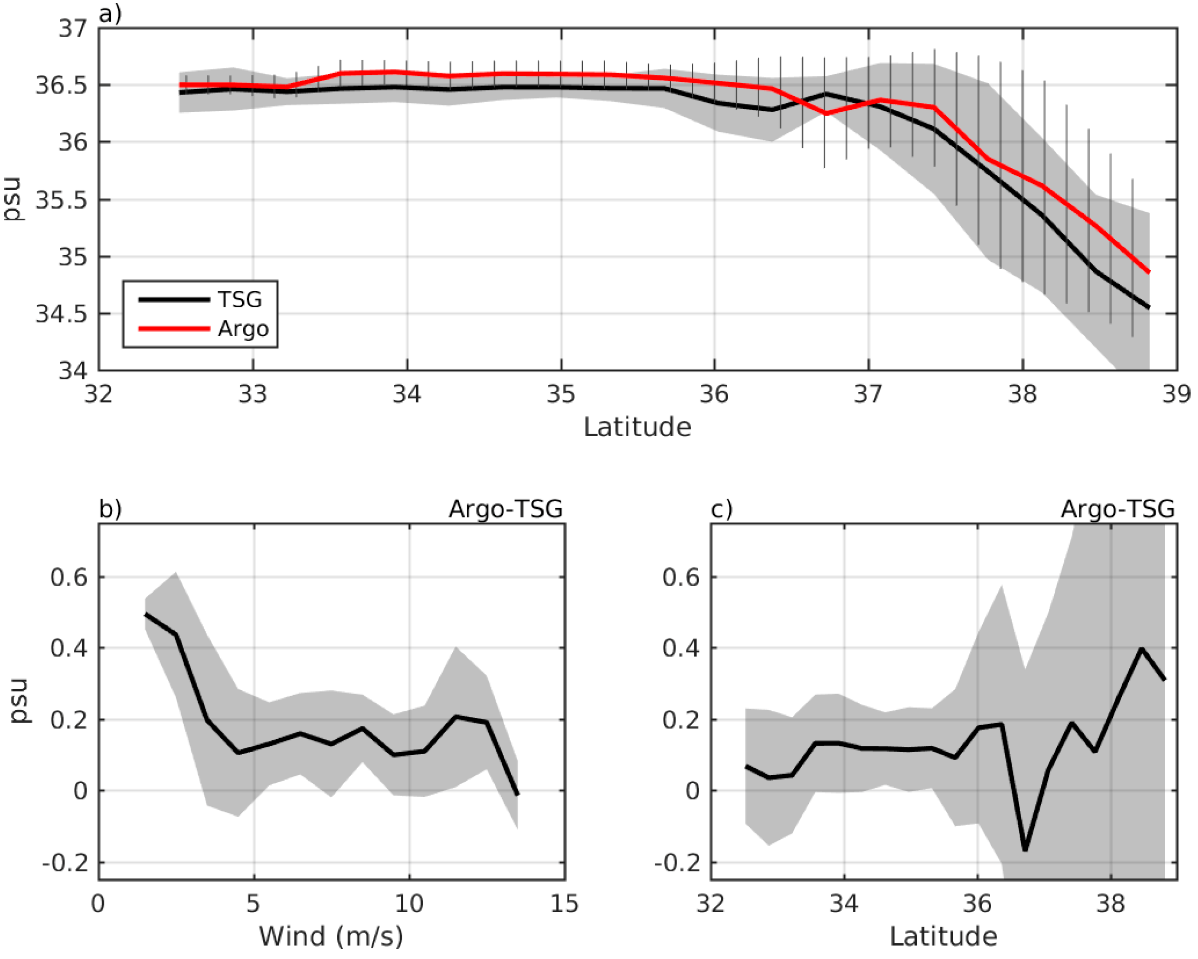
In an offshore segment of the OLEANDER transects (33°N LAT 37°N), where SRB should dominate, SMAP bias results show a slight overestimation during warm months and a clear underestimation in January-March (Figure 5). When averaged over the entire year, Figure 3b data suggest that these seasonal changes effectively cancel and lead to nearly unbiased SMAP SSS along this segment of the OLEANDER track. As noted before, this somewhat contradicts the time mean fresh bias versus Argo that is present in this area (Figure 2a). One possible reason for this disagreement could be the difference between TSG (~3 m) and Argo (5–10 m) measurement depths in combination with the presence of barrier layers and the associated shallow haline stratification known to prevail in this area (e.g., Liu et al. [22]). In fact, collocating TSG and Argo along the Oleander transects reveals that Argo is consistently saltier than TSG (Figure 6a) due to the stable near-surface halocline. The difference between Argo salinity and skin SSS (seen by SMAP and SMOS) would be expectably larger if there is a systematic salinity gradient above the Argo (5–10 m) and/or TSG measurement depths (~3 m). Binning Argo-TSG salinity difference versus wind speed (using only data from salinity homogeneous area south of the Gulf Stream and excluding Bermuda region, 33°N ≤ LAT ≤ 36°N), suggests that a fresh near-surface salinity contrast exists, and is largest (up to 0.5 psu) under calm winds (Figure 6b). This stratification will weaken when winds strengthen above m/s, but not completely. The mean Argo-TSG salinity difference remains psu ( 5 m/s), suggesting that at least a portion of the fresh SMAP bias seen in Figure 2a may be attributed to shallow stable haline stratification in rainy and river-impacted zones such as the NW Atlantic shelf. Figure 6a,c also indicate that near-surface halocline may be stronger in the high gradient area north of the Gulf Stream wall, where the lateral intrusion processes may contribute (e.g., Grodsky et al. [21]; Gawarkiewicz et al. [24]).
3.1.3. SMAP SSS Comparison with Mooring Data
Daily time series of near-surface salinity from buoys allow for a more complete temporal evaluation of SMAP SSS biases (Figure 7) at three regional sites. Haline stratification impacts on biases referenced to buoy measurements are expected to be weak, especially given that the seasonal cycle in regional haline impacts has been shown to be small (see Figure 5 in Li et al. [25]). The general physics of haline stratification above the shallowest buoy level, m, are discussed by Boutin et al. [26], but there is insufficient data to evaluate such shallow haline impacts quantitatively.
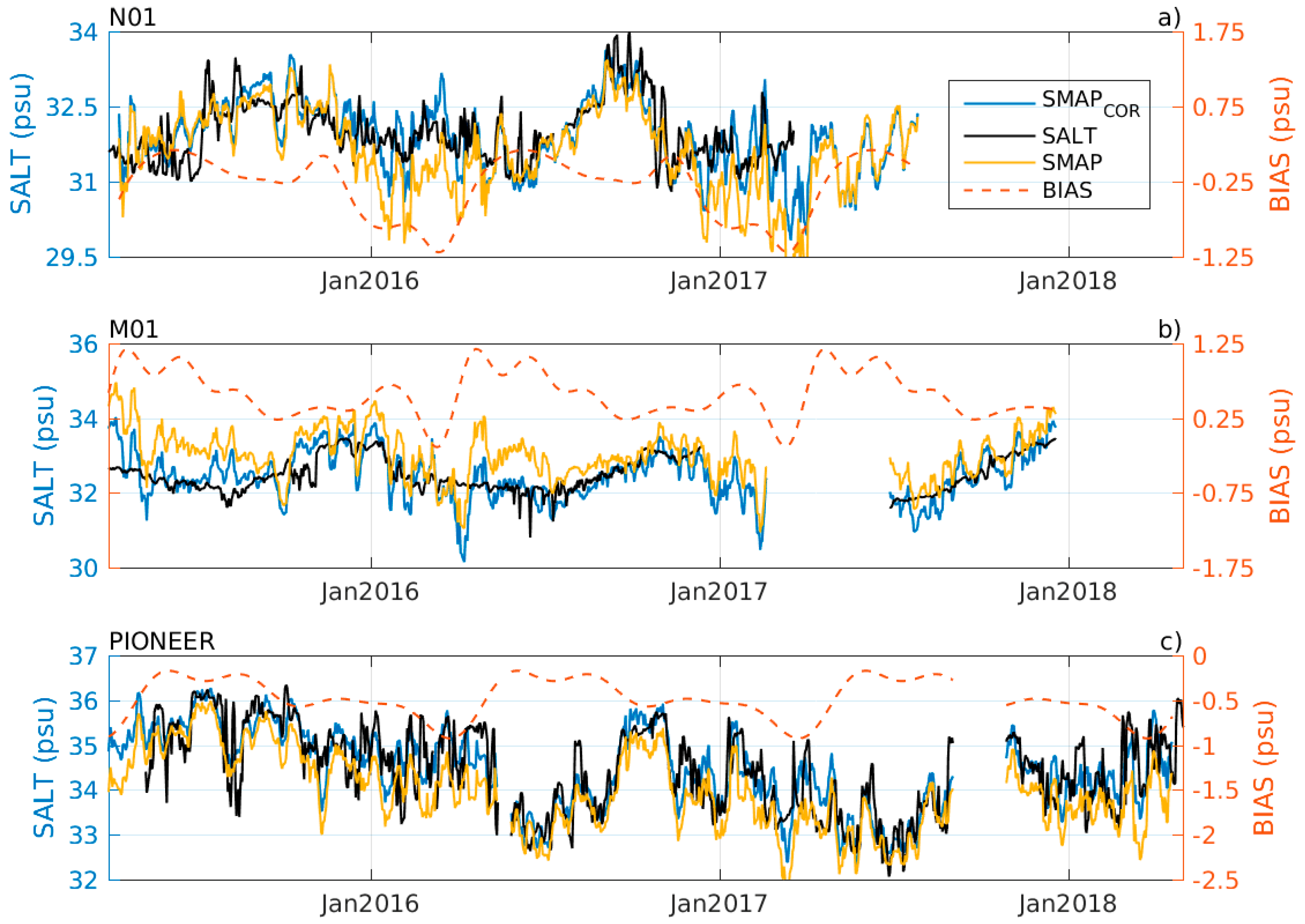
The SMAP biases referenced to 1-m buoy salinity, , exhibit clear seasonal variation around the annual mean bias at each node. The most negative bias values are in phase with the coldest SST typically occurring in February and March. This seasonal behavior is consistent among all of the buoys, and qualitatively agrees with the TSG-based results of Figure 5. NERACOOS buoy N01 (see Figure 1) is located near the entrance gate to the GoM where the land contamination is relatively low (). At N01, the seasonal SST varies from ~20 °C in summer down to ~5 °C in winter. During warm months, SMAP SSS closely follows the buoy data in Figure 7 to within some high frequency scatter. This contrasts with the cold season SMAP SSS, which is observed to be 1 psu fresher than in-situ . This appears to reflect an SST-dependent bias for coldest SST. The bias seasonal cycle is dominated by the first annual harmonic. Its removal largely corrects deviations between SMAP and buoy salinities, both decreasing the overall RMS difference and increasing temporal correlation between and (see Table 1). However, this seasonal debiasing doesn’t affect the high frequency (sampling) SMAP variability that is reflected in the high STD = 0.57 psu. The strong sampling variability of SMAP data results in the low correlation of daily SMAP and buoy salinity anomaly data (CORR = 0.25). This correlation between anomalies improves after monthly averaging of the data (CORR = 0.49). This indicates that SMAP SSS estimation noise is significantly reduced in monthly averages.
A similar error budget assessment at NERACOOS buoy M01 is more complex. In contrast to N01, where the SMAP retrieval bias (SRB) dominates, buoy M01 is located inside the GoM and closer to land. At M01, the LC bias component is stronger because the LC factor is near . Surprisingly, at this location, the strongest bias (~+1 psu) is observed in early summer, when SMAP SST impacts on SRB should weaken (Figure 7, M01). This seasonal behavior may reflect a combination of the SRB (negative in winter) and the LCB (positive except in boreal fall). Overall, the elevated positive bias at the M01 buoy is likely dominated by the positive LC component that arises due to overestimated land contamination effect at . During spring through fall, the SRB is small, and the total bias is close to the seasonal cycle of the local LCB, which is positive throughout the year and decreases in fall (in comparison with Figure 5). In winter to early spring, the positive LCB may be compensated by the negative SRB (Figure 7, M01). This possible cancellation effect could explain why SMAP SSS at the M01 location is more accurate in winter, just when SSS retrieval is most challenging.
The LC factor at the PIONEER offshore mooring site, (Figure 2a) predicts that SMAP SSS will be affected by both SRB and LCB (Figure 4b). Since the LC contamination overestimation dominates at larger , the LCB is expected to be negative here. A combination of the two bias components results in the negative total salinity bias (Figure 7, PIONEER). In summer, the SRB is expected to be small (similar to at N01 location, Figure 7, N01). Thus, the summer bias of psu is attributable to the LCB. Both bias components have stronger negative values during colder seasons. At the PIONEER offshore mooring, this leads to the seasonal peak in negative values of the total SMAP bias in winter through early spring ( psu).
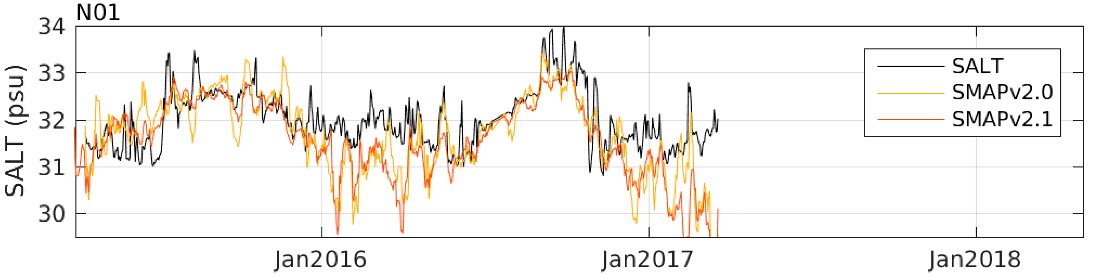
Very recently, the SMAP project released a new data version (2.1) intended for technical evaluation purposes only. This new version includes corrections that are meant to improve the SRB versus the SST. For completeness, we provide V2.0 versus V2.1 results in Figure 8. The data in Figure 7 and Figure 8 illustrate that these new SMAP SSS data at buoy N01 show very little SRB change in cold water conditions. One can observe that version 2.1 SMAP SSS is smoother (in time) in comparison with version 2.0 SSS. This difference is related to an effective 70-km spatial smoothing in version 2.1 (which is the only currently available). Since cold water SRB appears to be similar for the two versions, this study focuses on the publicly available SMAP version 2.0 datasets.
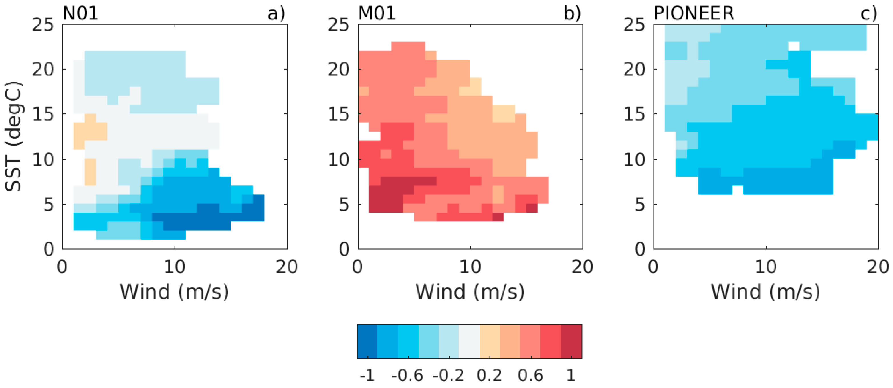
To further evaluate SRB characteristics, Figure 9 presents salinity differences binned in wind speed/SST space. The intent is to discern the remaining SRB signal due to either: (a) SST-dependent salinity sensitivity or (b) sea surface roughness (wave) effects on microwave emission and reflectance. The SRB structure is not easy to assess at the more coastal buoys (PIONEER and M01), because both LCB and SRB factor into the total SMAP bias, and both bias components have correlated seasonal variations. The bias component combination is evident at the M01 (Figure 9b), where, due to high , the total bias is dominated by the positive LCB.
At buoy N01, where LCB is weaker (), the total bias is close to the negative SRB. Its magnitude increases for cold SST and for stronger winds. Since these two factors are seasonally correlated, their relative impact is unclear, but their combination (cold SST and strong winds) leads to the most negative SRB levels (Figure 9a). A similar codependence is present at the PIONEER location () where negative values increase at low SST and strong winds. However, even during warm seasons, the total bias remains negative due to the contribution of negative LCB, which peaks at (Figure 4b).
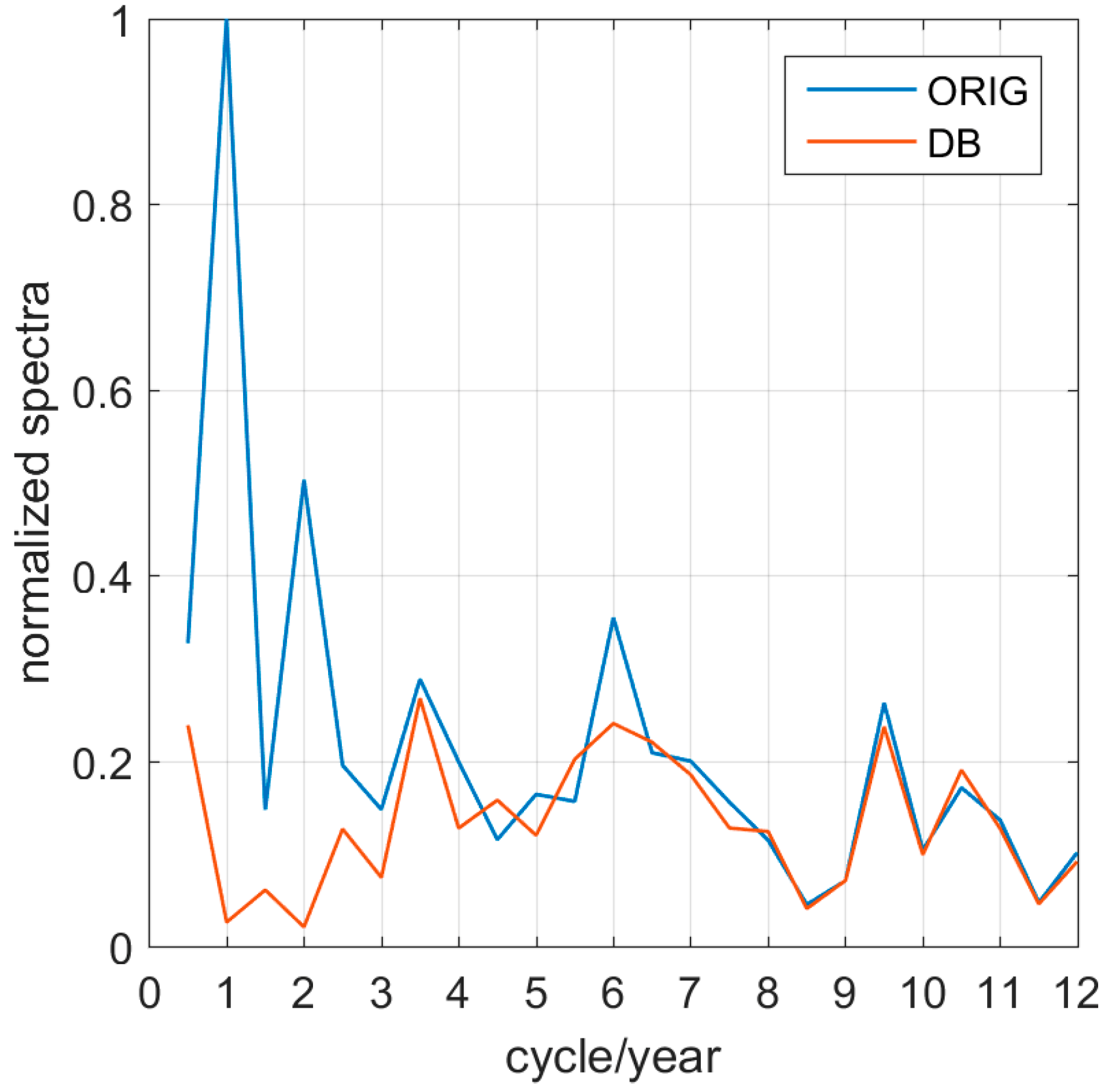
Annual and semiannual harmonics are the highest peaks in the spectrum of SMAP-BUOY salinity deviations (Figure 10). As expected, the removal of these annual peaks corrects for the most of the apparent deviations between SMAP and buoy, decreasing RMS salinity deviation and increasing the temporal correlation of collocated SMAP and buoy records (Table 1). However, the seasonal debiasing doesn’t affect the high frequency (sampling) SMAP variability that is reflected in the still high STD = 0.57 psu. The high frequency sampling variability present in the SMAP data results in the low correlation of daily anomalous salinity from SMAP and buoy (CORR ≈ 0.25, Table 1) except at the PIONEER, where interannual anomalies have larger amplitude than in the N01 and M01 records (Figure 7). However, the salinity anomaly skill improves after monthly averaging (CORR ≈ 0.5 at N01 and M01) due to the corresponding reduction in SMAP sampling variability. In the data discussion to follow, the anomalous SSS from SMAP will be used to monitor water exchanges between the GoM and the adjacent Atlantic shelf. In the data discussion to follow, these SMAP SSS anomaly estimates are used to evaluate the water exchange between the GoM and the adjacent Atlantic shelf.
3.1.4. SMAP SSS Comparison with Glider Data
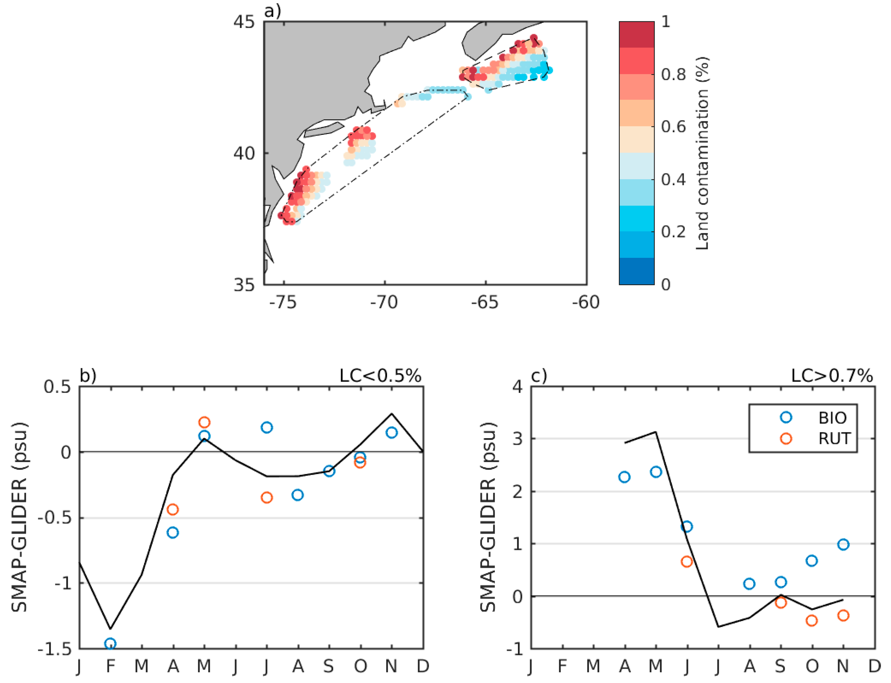
There are limited coincident glider and SMAP data matchups to augment SMAP LCB assessment. The available results are provided in Figure 11. The data are focused on two regions, as shown in Figure 11a. The results of SMAP-glider S differences are stratified into ad hoc seaward (LC < 0.5%) and coastal (LC > 0.7%) cases based on the LC impacts shown earlier using the TSG datasets. Seaward data in Figure 11b exhibit a seasonal cycle in SMAP bias that resembles the SRB shown earlier. It is weak year round, but strong ( psu) negative values are present in the phase with cold SST during winter to early spring. This is consistent with buoy (Figure 7 and Figure 9) and TSG (Figure 5) comparisons. Coastal data, as shown in Figure 11c, exhibit strong positive LCB values (associated with an overestimation of the LC effect) in the first half of the year. This bias component is significantly attenuated during the second half of the year, which is in contrast with the OLEANDER data (Figure 5) that exhibit weaker positive LCB values only in the fall. This seasonal behavior is mostly dictated by the Bedford Institute of Oceanography (BIO) glider data on the more northern Scotian Shelf region. These data have better seasonal coverage than the Rutgers University glider data collected to the southwest (Figure 11c). It may be not surprising to see the difference in LCB seasonality between the Nova Scotia shelf (Figure 11b) and Mid-Atlantic Bight (Figure 5) due to differing ocean brightness temperatures and terrestrial properties.
3.2. Applying SMAP Data to Gulf of Maine SSS Monitoring
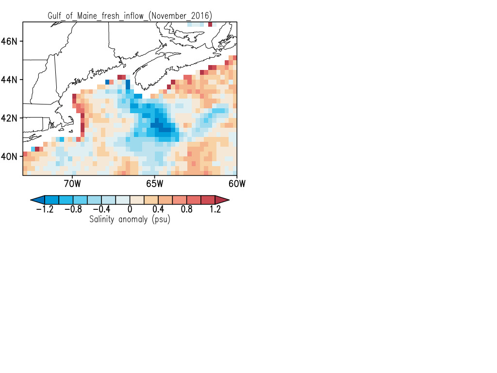
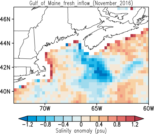
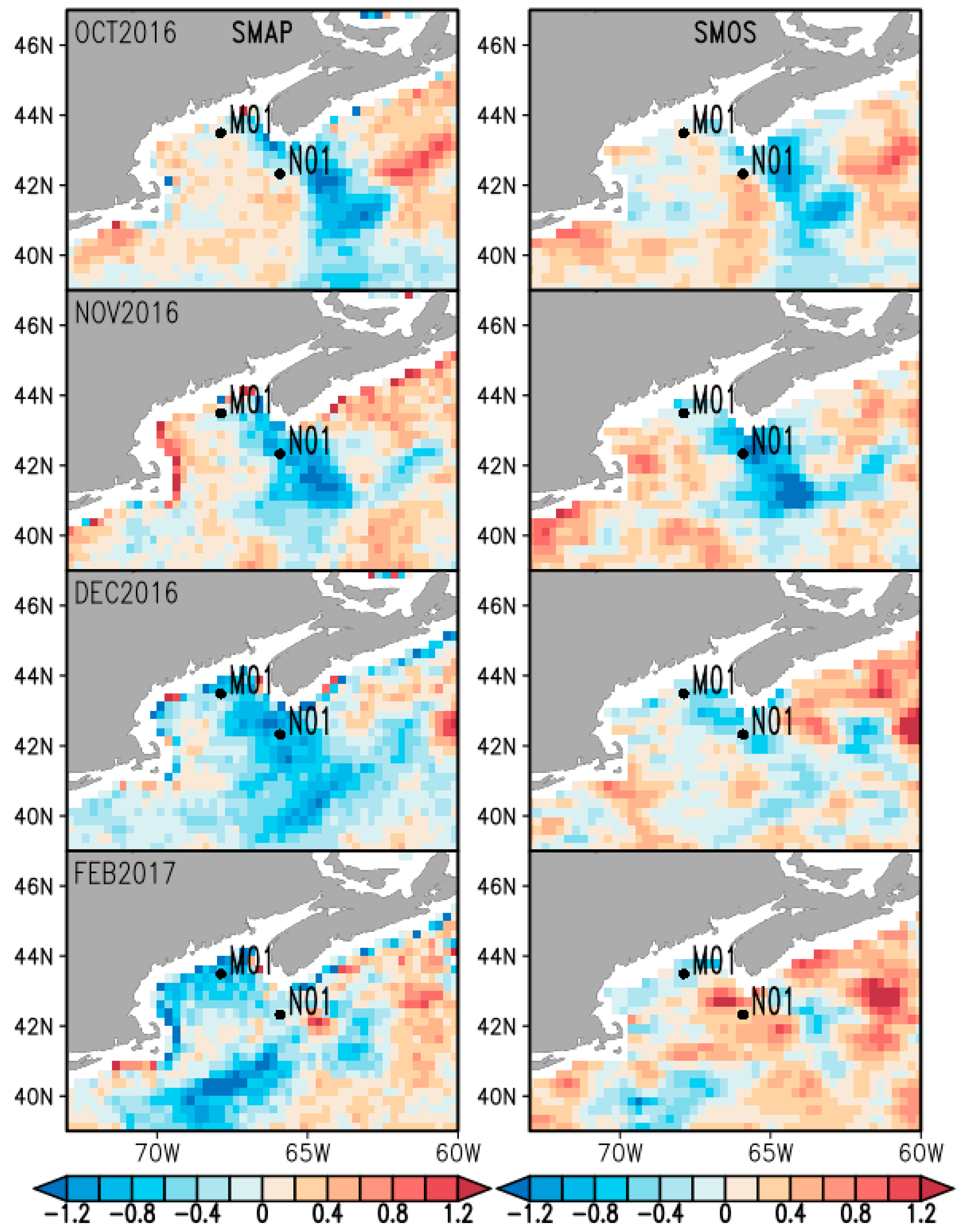
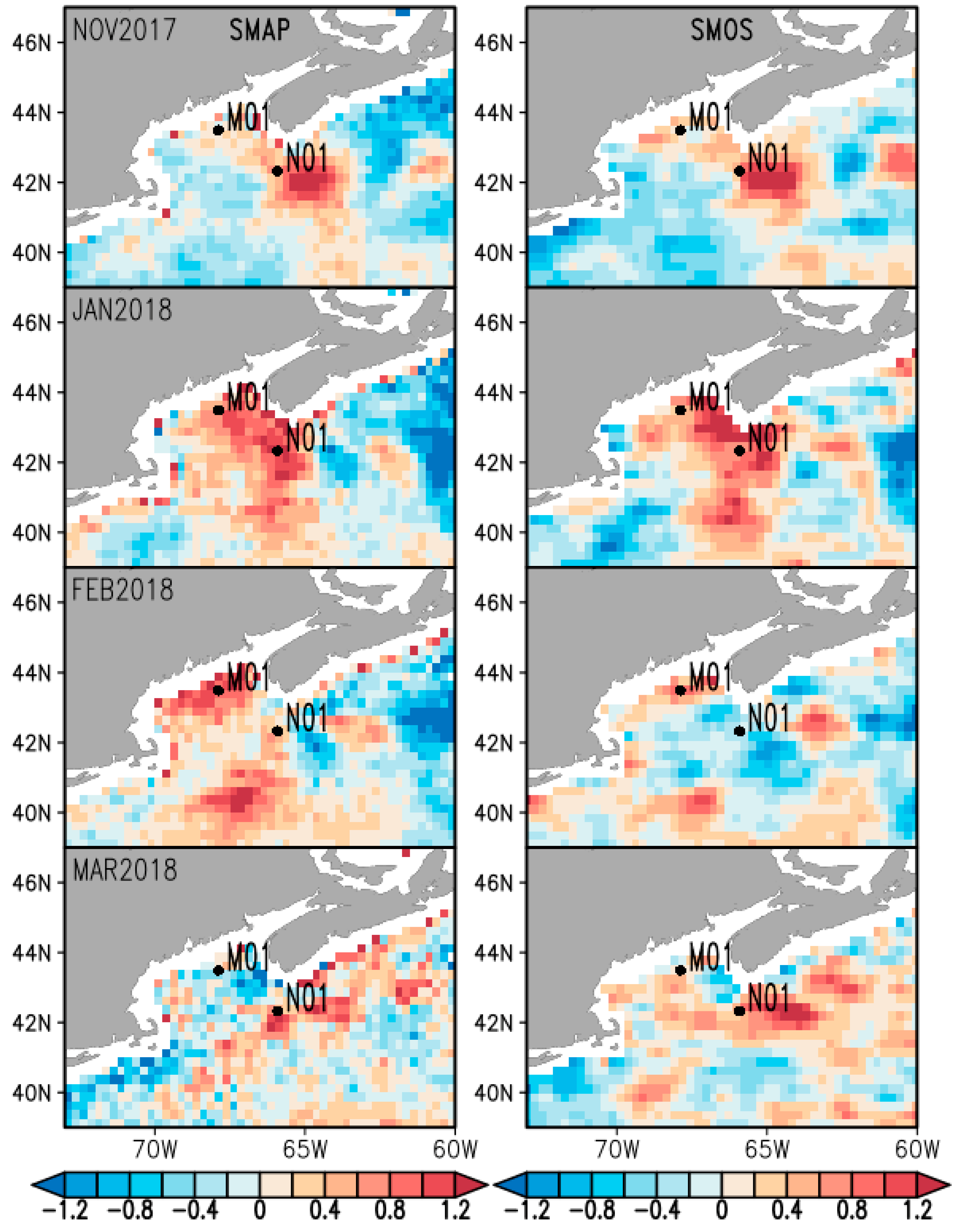
Spatial SST gradients in the Gulf of Maine region are significantly reduced during the winter due to strong near-surface mixing and destratification. This, in part, helps to open a gateway for winter period water exchanges with the adjacent NW Atlantic shelf. During the winters of 2016/17 and 2017/18, monthly SMAP SSS anomaly (SSSA) data indicate two differing episodes of Gulf of Maine water inflow (Figure 12 and Figure 13). In both winters, there is the localized intensity of SSSA anomalies fields near the inflow pathways in between Georges Banks and Nova Scotia (i.e., near buoy station N01, see also Figure 2b). Figure 12 and Figure 13 also show that the SSSA patterns observed by SMAP are remarkably consistent with the independent measurements produced using the European Soil Moisture Ocean Salinity (SMOS) mission sensor. This lends confidence to the SMAP-observed phenomena. The dynamics and details tied to the high salinity feature observed in January and February 2018 (Figure 13) are the subject of a separate study, and are thus not discussed further here. Here, we focus on the apparent freshwater inflow to the GoM in winter 2016/17.
The initial stage of the fresh GoM inflow is evident in October 2016 as an anomalous SSS pattern that shows a tongue of low SSS entering the GoM along the southwestern Nova Scotia coast (Figure 12). The pattern is consistent in SMAP and SMOS data. Notably, the SSSA (salinity anomaly) front lies northeast of buoy N01, meaning upstream of the Northeast Channel (NEC), which is the main gateway for winter shelf and slope water inflows that normally penetrate the GoM as deeper inflow (Ramp et al. [5]). In this case, the October 2016 fresh anomaly does not involve NEC transport, at least at this stage. By November 2016 (Figure 12), the core of the low SSSA feature near the NEC still lies northeast of buoy N01 and the NEC. Moreover, the fresh pattern is shifted closer to the Cape Sable coast, which is consistent with inflow through the Northern Channel (see Figure 2b) and inflow through the interior of the GoM.
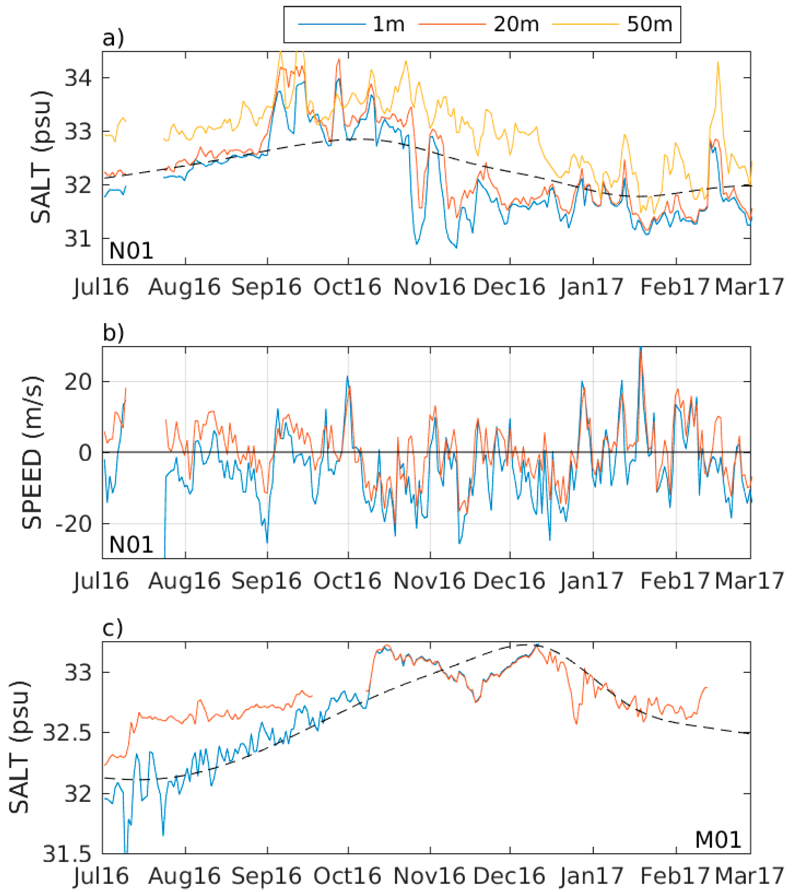
In situ observations from buoy N01 show that first evidence of near-surface freshening at this site is observed in late October 2016 (Figure 14a). The fresh intrusion (more than −1 psu) is evident to at least 20-m depth in the water column, but doesn’t penetrate down to 50 m. This anomalously freshwater is present in the surface layers of the NEC through January 2017. The spatial SSSA SMAP data suggest this freshwater intrusion is not advected into the NEC from the Atlantic to the southeast, but is probably a lateral diffusion of the upstream (poleward) main fresh feature located to the northeast of the NEC. This hypothesis is consistent with the upper ocean currents measured at N01 (Figure 14b). The upper 20-m velocity data show a generally southwest (SW) (down channel) NEC flow (negative velocity components, in line with Brooks [27]) during this fresh feature entrance period (October 2016 to January 2017).
From December 2016 through February 2017, the Figure 12 correspondence between SMAP and SMOS SSS anomalies is not as clear. We posit that this is probably due to SMOS debiasing issues. During this period, SMAP data show that anomalously freshwater occupies a significant portion of the northeastern GoM (December 2016). In February 2017, it starts circulating cyclonically along the northwestern Gulf coast in the Maine Coastal Current, while the open ocean part of the fresh anomaly travels further down shelf along the shelf–slope current. In situ buoy data from station M01, located inside the GoM, confirm that transient fresh SSS anomalies of ~ psu are observed in the upper 20-m water column during November and December 2016 (Figure 14c), which is consistent with SMAP data. However, the 20-m depth M01 data in January and February 2017 indicate that salinity at the M01 is close to the normal, which is at odds with the strong negative SSSA in the last SMAP panel of Figure 12 at site M01. Unfortunately, the M01 surface (1-m) salinity data are unavailable after mid-December 2016. Overall, the N01 and M01 buoy data certainly confirm the timing and general magnitude of a near-surface freshening in the GoM from at least October into December 2016.
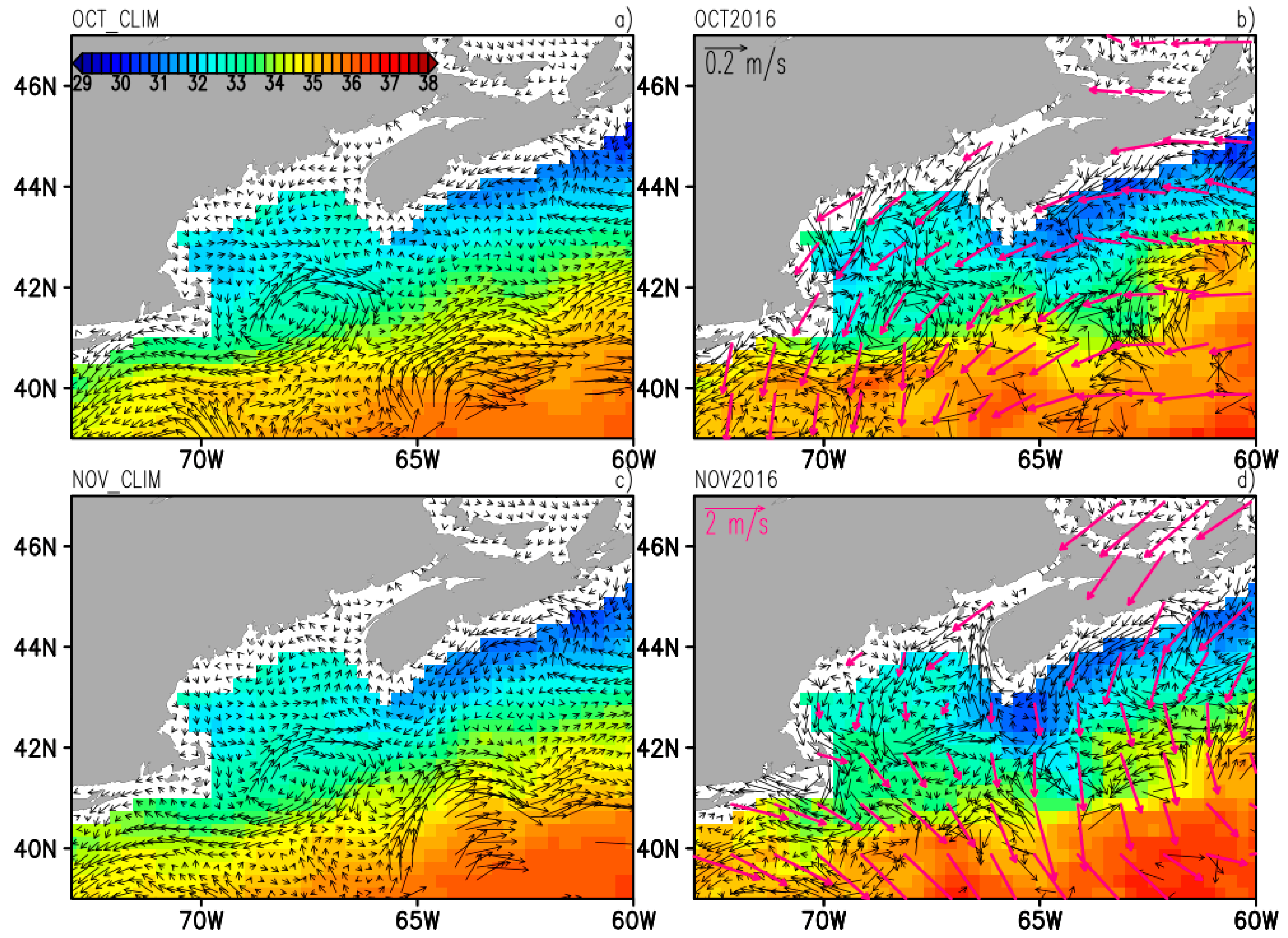
Next, we consider a possible scenario of dynamical events leading to this local 2016/17 winter fresh inflow. The freshest water in the region is known to be present along the southeastern Nova Scotia coast (Figure 15). It is transported southwestward down the coast within the Scotian Shelf Current (SSC, inshore branch). The variability of this coastal transport is an important factor controlling freshwater inflows into the GoM (Feng et al. [3]). To assess this as a possible explanation for the observed SMAP SSSA data near buoys N01 and M01, we present climatological and anomalous ocean current and wind data for October and November 2016 in Figure 15. The climatological geostrophic currents along the SSC (~65°W, 43.5°N in Figure 15a,c) are apparently weaker than the SSC current in fall of 2016 (Figure 15b,d). These anomalously strong currents result in stronger coastal volume transport and thus lower salinity around the southern tip of Nova Scotia (Figure 15). Moreover, the dynamical forcing relevant to this SSC acceleration may be related to wind forcing. During October and November 2016, the satellite scatterometer wind data depict a southwestward wind anomaly over the NW Atlantic (Figure 15b,d). Such a wind anomaly reflects a weakening of prevailing alongshore westerly winds on the shelf near southeastern Nova Scotia. The associated coastal sea level set up enhances the cross-coastal sea level gradient, increasing the SSC following the valve mechanism suggested by Li et al. [25].
The positive wind-induced sea level anomaly evolves southwestward along the Nova Scotia coast as a coastal western boundary Kelvin wave that distributes the sea level high further south and thus accelerates the SSC around the entire southern part of Nova Scotia. In November 2016, the accelerated SSC encompassed Nova Scotia and branched its freshwaters into the GoM (Figure 15d). This is also coincident with cyclonic anomalous upwelling wise winds over the GoM (Figure 15d) that depress in-Gulf sea levels and additionally contribute to coastal currents acceleration and the resulting anomalously strong freshwater inflow.
4. Conclusions
This paper addresses several challenging issues related to satellite ocean salinity data accuracy and application within the challenging salinity remote sensing domains of both cold and coastal waters. The focus region is the Gulf of Maine and the adjoining Scotian Shelf and NW Atlantic shelf break, where upstream fresh coastal subarctic waters are advected into a region that also includes high salinity Gulf Stream eddies. Both can lead to strong salinity gradients and variable water mass exchanges that are often best identified using salinity fields rather than temperature. An extensive regional approach to SMAP SSS data accuracy assessment is provided using not only Argo data (which do not collect data in shelf and coastal areas) but also all of the available in situ measurements. The paper also examines anomalous salinity signatures propagating into the productive waters of the Gulf of Maine (GoM) to assess their interactions with the nearby NW Atlantic shelf.
A regional SMAP SSS error assessment exposes remaining SSS bias using a suite of near-surface salinity measurements that includes buoy, thermosalinograph (TSG), and glider data. For the NW Atlantic, our analysis shows that SMAP SSS is subject to an SST-dependent bias that is negative and at its maximum in winter and early spring (up to psu). Our speculation is that this is due to the SST-related decrease in microwave sensor sensitivity to SSS when SST falls below 5–7 °C. The data also indicate that regional SMAP SSS is subject to a land contamination bias associated with the contribution of land radiation via side lobes of SMAP antenna. The latter bias is identified by comparing SMAP SSS with salinity data from repeating M/V OLEANDER TSG ship transects. SSS differences are found to be a function of the antenna land contamination factor (LC), becoming significant and negative for 0.2%. Maximum negative SSS biases near psu occur for . Coastward, a very different SMAP SSS bias arises for , where a larger and positive land contamination bias grows to reach psu. This near coastal positive land contamination bias is probably related to a local overestimation of land contamination impact along the M/V OLEANDER line. However, while this land contamination bias is expected to be regionally dependent due to geographic changes in the difference between land and sea microwave radiation, a qualitatively similar land contamination bias is also observed along the distant M/V NUKA-ARCTICA Europe-to-Greenland repeating transects, which are further north near 60°N.
Data also indicate that SMAP SSS bias components related to SST correction and land contamination are seasonally dependent. We attribute this to seasonal changes in SST/winds and coastal terrestrial microwave emissivity. Seasonal harmonics are the highest peaks in spectra of SMAP-TSG salinity difference. As for the other open ocean satellite SSS studies, the results show that a pragmatic remedy to work around these SSS bias issues is the computation and use of SMAP SSS anomalies; anomalies are formed taking the difference relative to a satellite SSS climatology. The approach effectively removes seasonal biases along with the real seasonal cycle, but provides access to spatial and temporal information on interannual SSS change. The NW Atlantic SMAP results shown in Table 1 and Figure 12 and Figure 13 suggest that SMAP monthly SSS anomalies have sufficient accuracy and applicability to allow new insight into shelf and coastal dynamics at the monthly scale. Satellite data for 2015–2018 were used to examine Gulf of Maine water inflow, with data suggesting distinct and important water intrusions localized between Georges Banks and Nova Scotia in the winters of 2016/17 and 2017/18. Water intrusion patterns observed by SMAP are consistent with independent measurements from the European SMOS mission.
A cursory evaluation of the dynamics of the winter 2016/17 freshening anomaly inflow used satellite-based ocean current and wind vector data (Figure 15) to suggest the change is controlled by an anomalously strong increase in the Scotian Shelf Current (SSC) that transports Scotian Shelf Water (the freshest water in the region) southwestward down the coast. This results in lower salinity around the southern tip of Nova Scotia, and stronger coastal freshwater flux into the GoM that agrees with interior GoM buoy salinity data at station M01. The forcing behind this SSC acceleration is likely wind-driven in that wind anomaly data in October and November 2016 are consistent with a relaxation in the prevailing Scotian Shelf alongshore westerlies. This finding generally agrees with the circulation perturbation mechanism discussed recently in Li et al. [25].
In summary, study results indicate favorable possibilities for both the immediate use and future improvement of SMAP surface salinity measurements along the slope and sea regions of the NW Atlantic. The new regional in situ datasets compiled to help evaluate coastal and cold-water SMAP data accuracy issues clearly add new information to support improvements of the data processing algorithms, as well as validation data to support the use of salinity anomaly datasets for scientific applications using the presently available V2.0 SMAP data.
Author Contributions
Conceptualization and Methodology, S.A.G. and D.V.; Writing-Original Draft Preparation, S.A.G.; Glider data processing, H.F.
Funding
This research is supported by the NASA Earth Science Division via Ocean Salinity Science Team funding (OSST grants NNX17AK08G and NNX17AK02G).
Acknowledgments
SMAP salinity is produced by Remote Sensing Systems and sponsored by the NASA OSST. NERACOOS and OOI projects are acknowledged for providing the buoy hydrographic data. The glider operations are funded by the Ocean Tracking Network (OTN) and the Marine Environmental Observation Prediction and Response Network (MEOPAR). MAB Slocum glider datasets are provided by the Rutgers University COOL group. Argo data were collected and made freely available by the International Argo Program and the national programs that contribute to it (http://www.argo.ucsd.edu, http://argo.jcommops.org). The Argo Program is part of the Global Ocean Observing System. TSG salinity data are provided by the LEGOS SSS observation service (http://www.legos.obs-mip.fr/observations/sss/) and by the OLEANDER Project (http://po.msrc.sunysb.edu/Oleander/TSG/TSG.html).
Conflicts of Interest
The authors declare no conflict of interest.
References
- Mountain, D.G. Labrador slope water entering the Gulf of Maine-response to the North Atlantic Oscillation. Cont. Shelf Res. 2012, 47. [Google Scholar] [CrossRef]
- Townsend, D.W.; Pettigrew, N.R.; Thomas, M.A.; Neary, M.G.; Mcgillicuddy, D.J.; Donnell, J.O. Water masses and nutrient sources to the Gulf of Maine. J. Mar. Res. 2015, 73. [Google Scholar] [CrossRef] [PubMed]
- Feng, H.; Vandemark, D.; Wilkin, J. Gulf of Maine salinity variation and its correlation with upstream Scotian Shelf currents at seasonal and interannual time scales. J. Geophys. Res. Ocean. 2016, 121. [Google Scholar] [CrossRef]
- Peterson, I.; Greenan, B.; Gilbert, D.; Hebert, D. Variability and wind forcing of ocean temperature and thermal fronts in the Slope Water region of the Northwest Atlantic. J. Geophys. Res. Oceans 2017, 122. [Google Scholar] [CrossRef]
- Ramp, S.R.; Schlitz, R.J.; Wright, W.R. The Deep Flow through the Northeast Channel, Gulf of Maine. J. Phys. Oceanogr. 1985, 15. [Google Scholar] [CrossRef]
- Grodsky, S.A.; Reul, N.; Chapron, B.; Carton, J.A.; Bryan, F.O. Interannual surface salinity on Northwest Atlantic shelf. J. Geophys. Res. Oceans 2017, 122. [Google Scholar] [CrossRef]
- Reul, N.; Chapron, B.; Lee, T.; Donlon, C.; Boutin, J.; Alory, G. Sea surface salinity structure of the meandering Gulf Stream revealed by SMOS sensor. Geophys. Res. Lett. 2014, 41. [Google Scholar] [CrossRef]
- Dinnat, E.P.; Le Vine, D.M. Effects of the Antenna Aperture on Remote Sensing of Sea Surface Salinity at L-Band. IEEE Trans. Geosci. Remote Sens. 2007, 45, 2051–2060. [Google Scholar] [CrossRef]
- Gierach, M.M.; Vazquez-Cuervo, J.; Lee, T.; Tsontos, V.M. Aquarius and SMOS detect effects of an extreme Mississippi River flooding event in the Gulf of Mexico. Geophys. Res. Lett. 2013, 40, 5188–5193. [Google Scholar] [CrossRef] [Green Version]
- Köhler, J.; Sena Martins, M.; Serra, N.; Stammer, D. Quality assessment of spaceborne sea surface salinity observations over the northern North Atlantic. J. Geophys. Res. Oceans 2015, 120, 94–112. [Google Scholar] [CrossRef] [Green Version]
- Meissner, T.; Wentz, F.J.; Scott, J.; Vazquez-Cuervo, J. Sensitivity of Ocean Surface Salinity Measurements From Spaceborne L-Band Radiometers to Ancillary Sea Surface Temperature. IEEE Trans. Geosci. Remote Sens. 2016, 54, 7105–7111. [Google Scholar] [CrossRef]
- Tang, W.; Fore, A.; Yueh, S.; Lee, T.; Hayashi, A.; Sanchez-Franks, A.; Martinez, J.; King, B.; Baranowski, D. Validating SMAP SSS with in situ measurements. Remote Sens. Environ. 2017, 200, 326–340. [Google Scholar] [CrossRef]
- Boutin, J.; Martin, N.; Kolodziejczyk, N.; Reverdin, G. Interannual anomalies of SMOS sea surface salinity. Remote Sens. Environ. 2016, 128–136. [Google Scholar] [CrossRef]
- Lee, T. Consistency of Aquarius sea surface salinity with Argo products on various spatial and temporal scales. Geophys. Res. Lett. 2016, 43, 3857–3864. [Google Scholar] [CrossRef]
- Kubryakov, A.; Stanichny, S.; Zatsepin, A. River plume dynamics in the Kara Sea from altimetry-based lagrangian model, satellite salinity and chlorophyll data. Remote Sens. Environ. 2016, 176, 177–187. [Google Scholar] [CrossRef]
- Garcia-Eidell, C.; Comiso, J.C.; Dinnat, E.; Brucker, L. Satellite observed salinity distributions at high latitudes in the Northern Hemisphere: A comparison of four products. J. Geophys. Res. Ocean. 2017, 122, 7717–7736. [Google Scholar] [CrossRef]
- Meissner, T.; Wentz, F.J. Remote Sensing Systems SMAP Ocean Surface Salinities [Level 2C, Level 3 Running 8-day, Level 3 Monthly], Version 2.0 Validated Release; Remote Sensing Systems: Santa Rosa, CA, USA, 2016. [Google Scholar]
- Boutin, J.; Vergely, J.L.; Marchand, S.; D’Amico, F.; Hasson, A.; Kolodziejczyk, N.; Reul, N.; Reverdin, G.; Vialard, J. New SMOS Sea Surface Salinity with reduced systematic errors and improved variability. Remote Sens. Environ. 2018, 214, 115–134. [Google Scholar] [CrossRef]
- Tang, W.; Yueh, S.; Yang, D.; Fore, A.; Hayashi, A.; Lee, T.; Fournier, S.; Holt, B. The Potential and Challenges of Using Soil Moisture Active Passive (SMAP) Sea Surface Salinity to Monitor Arctic Ocean Freshwater Changes. Remote Sens. 2018, 10, 869. [Google Scholar] [CrossRef]
- Bentamy, A.; Fillon, D.C. Gridded surface wind fields from Metop/ASCAT measurements. Int. J. Remote Sens. 2012, 33, 1729–1754. [Google Scholar] [CrossRef]
- Grodsky, S.A.; Carton, J.A.; Liu, H. Comparison of bulk sea surface and mixed layer temperatures. J. Geophys. Res. Oceans 2008, 113. [Google Scholar] [CrossRef] [Green Version]
- Liu, H.; Grodsky, S.A.; Carton, J.A. Observed subseasonal variability of oceanic barrier and compensated layers. J. Clim. 2009, 22, 6104–6119. [Google Scholar] [CrossRef]
- Song, Y.T.; Lee, T.; Moon, J.H.; Qu, T.; Yueh, S. Modeling skin-layer salinity with an extended surface-salinity layer. J. Geophys. Res. Oceans 2015, 120, 1079–1095. [Google Scholar] [CrossRef] [Green Version]
- Gawarkiewicz, G.; Todd, R.; Zhang, W.; Partida, J.; Gangopadhyay, A.; Monim, M.-U.-H.; Fratantoni, P.; Malek Mercer, A.; Dent, M. The Changing Nature of Shelf-Break Exchange Revealed by the OOI Pioneer Array. Oceanography 2018, 31, 60–70. [Google Scholar] [CrossRef] [Green Version]
- Li, Y.; Ji, R.; Fratantoni, P.S.; Chen, C.; Hare, J.A.; Davis, C.S.; Beardsley, R.C. Wind-induced interannual variability of sea level slope, along-shelf flow, and surface salinity on the Northwest Atlantic shelf. J. Geophys. Res. Oceans 2014, 119, 2462–2479. [Google Scholar] [CrossRef] [Green Version]
- Boutin, J.; Chao, Y.; Asher, W.E.; Delcroix, T.; Drucker, R.; Drushka, K.; Kolodziejczyk, N.; Lee, T.; Reul, N.; Reverdin, G.; et al. Satellite and in situ salinity understanding near-surface stratification and subfootprint variability. Bull. Am. Meteorol. Soc. 2016, 97, 1391–1407. [Google Scholar] [CrossRef]
- Brooks, D.A. The influence of warm-core rings on slope water entering the Gulf of Maine. J. Geophys. Res. 1987, 92, 8183. [Google Scholar] [CrossRef]
Figure 1.
(a) Time mean Soil Moisture Active Passive (SMAP) minus Array for Real-Time Geostrophic Oceanography (Argo) salinity differences (PSU) over the northwestern (NW) Atlantic shelf. SMAP antenna land contamination (%) is shown in coastal areas. Data gaps are shaded in gray. The Oleander ship transect (dashed), PIONEER buoy, M01 and N01 NERACOOS buoy sites are overlain. (b) Gulf of Maine (GoM) and adjacent area bathymetry. Buoy locations are shown in magenta. The geographic area of panel (b) is marked by the box in panel (a).

Figure 2.
(a) Time mean (April 2015–April 2018) of a daily salinity difference of one degree, SMAP-Argo SMAP antenna land contamination 0.2% contour is shown. (b) Time-latitude diagram of zonally averaged SMAP-Argo. Zonally averaged 20C, 25C, and 27C SST contours are overlain.
Figure 2.
(a) Time mean (April 2015–April 2018) of a daily salinity difference of one degree, SMAP-Argo SMAP antenna land contamination 0.2% contour is shown. (b) Time-latitude diagram of zonally averaged SMAP-Argo. Zonally averaged 20C, 25C, and 27C SST contours are overlain.

Figure 3.
(a) Sample regional SMAP sea surface salinity (SSS) data and mapping of the M/V OLEANDER transect line. Also shown are SMAP data product estimates for land contamination given as contours at 0.2%, 0.5%, and 0.8%. (b) Time mean SMAP SSS, thermosalinograph (TSG) salinity, and antenna land contamination (Gland). Gray shading and vertical bars are standard deviations of TSG and SMAP salinity, respectively.

Figure 4.
(a) Geographical map of M/V OLEANDER and NUKA-ARCTICA transects. (b) SMAP-TSG salinity difference binned versus land contamination factor (LC) for the two ship datasets. Data scatter (STD) in each 0.1% bin is shown by vertical and horizontal lines for M/V OLEANDER and NUKA-ARCTICA, respectively.

Figure 5.
Latitude calendar month diagram of SMAP-TSG salinity difference along the OLEANDER line. So far, there are no August OLEANDER TSG data during the SMAP period.
Figure 5.
Latitude calendar month diagram of SMAP-TSG salinity difference along the OLEANDER line. So far, there are no August OLEANDER TSG data during the SMAP period.

Figure 6.
(a) Time mean salinity difference between Argo (5–10 m) and TSG (~3 m) along the OLEANDER line. Data scatter (STD) in each 0.5° latitude bin is shown by gray shading and vertical lines for TSG and Argo, respectively. (b) Argo-TSG south of 36N as a function of wind speed. (c) Argo-TSG as a function of latitude. Data scatter (STD) is shown by gray shading in (b,d).

Figure 7.
Buoy 1-m salinity (SALT), SMAP salinity, and SMAP salinity corrected for the seasonal bias (SMAPCOR). Seasonally dependent BIAS=SMAP-BUOY is shown against the right hand vertical axis. (a,b) show data from NorthEastern Regional Association of Coastal and Ocean Observing Systems (NERACOOS) moorings N01 and M01. (c) shows data from OOI PIONEER mooring.

Figure 8.
Buoy N01 1-m salinity (SALT), SMAP version 2.0 and version 2.1 collocated salinity.

Figure 9.
SMAP-BUOY salinity bias binned versus SST and wind speed for (a,b) NERACOOS moorings N01 and M01, and (c) OOI PIONEER mooring.
Figure 9.
SMAP-BUOY salinity bias binned versus SST and wind speed for (a,b) NERACOOS moorings N01 and M01, and (c) OOI PIONEER mooring.

Figure 10.
Spectrum of SMAP-S (z = 1 m) difference for original (ORIG) and debiased (DB) SMAP SSS. Spectra for N01, M01, and PIONEER data are averaged after normalization on their spectrum peak values. Spectra based on debiased data are normalized on the same peak values of original spectra.
Figure 10.
Spectrum of SMAP-S (z = 1 m) difference for original (ORIG) and debiased (DB) SMAP SSS. Spectra for N01, M01, and PIONEER data are averaged after normalization on their spectrum peak values. Spectra based on debiased data are normalized on the same peak values of original spectra.

Figure 11.
(a) Glider coverage for Bedford Institute of Oceanography (BIO) data near Nova Scotia and Rutgers University (RUT) data in the Mid-Atlantic Bight. Colors represent SMAP antenna land contamination (LC, %). (b) SMAP-GLIDER bias binned each calendar month for LC < 0.5%. (c) SMAP-GLIDER bias in the coastal regions with strong land contamination (LC > 0.7%). The black curves in (b,c) are the seasonal fit with the first three annual harmonics. Only calendar months with at least 10 collocated data are used.

Figure 12.
Anomalous SSS from (left) SMAP and (right) Soil Moisture Ocean Salinity (SMOS) during the fall and winter of 2016–2017.
Figure 12.
Anomalous SSS from (left) SMAP and (right) Soil Moisture Ocean Salinity (SMOS) during the fall and winter of 2016–2017.

Figure 13.
Anomalous SSS from (left) SMAP and (right) SMOS during the fall and winter of 2017–2018.

Figure 14.
Time series of (a) salinity and (b) currents at buoy N01 located in the Northeastern Channel. Currents are projected on the direction perpendicular to the general orientation of the coast (30 degrees counterclockwise from the true north). Positive currents correspond to Gulf of Maine inflow along the Northeastern Channel. (c) Time series of salinity at buoy M01. Climatological salinity at z = 1 m is shown as black dashed line. The x-axis labels correspond to the first day of the month.

Figure 15.
SMOS SSS (shaded) and surface geostrophic currents (black arrows) during the fresh feature entrance to the Gulf of Maine in October and November 2016 (see Figure 12). The left column (a,c) shows climatological conditions for October and November 2016. The right column (b,d) shows conditions for October and November 2016. Advanced Scatterometer (ASCAT) anomalous wind for October and November 2016 is overlaid in panels (b,d), respectively. For simplicity, debiased SMOS (rather than SMAP) is used for absolute SSS, because all of the near coastal grid points, which are subject to strong bias, are filtered out from this product.


Table 1.
Comparison of the daily mean buoy (z = 1 m) and collocated SMAP salinity (black/red is for original/corrected SMAP SSS, respectively). Correlation (CORR) of buoy vs. SMAP salinity anomalies (SSSA) is included in the last two columns for monthly and daily anomalies. See Figure 2 for buoy locations.
| BUOY | BIAS (psu) SMAP-BUOY | RMS (psu) | STD (psu) | CORR | Monthly Anomaly CORR | Daily Anomaly CORR |
|---|---|---|---|---|---|---|
| N01 | −0.34 | 0.80/0.57 | 0.72/0.57 | 0.56/0.63 | 0.49 | 0.25 |
| M01 | 0.56 | 0.68/0.29 | 0.43/0.29 | 0.62/0.84 | 0.58 | 0.27 |
| PIONEER | −0.48 | 0.77/0.57 | 0.61/0.57 | 0.77/0.80 | 0.97 | 0.76 |
© 2018 by the authors. Licensee MDPI, Basel, Switzerland. This article is an open access article distributed under the terms and conditions of the Creative Commons Attribution (CC BY) license (http://creativecommons.org/licenses/by/4.0/).
Share and Cite
MDPI and ACS Style
Grodsky, S.A.; Vandemark, D.; Feng, H. Assessing Coastal SMAP Surface Salinity Accuracy and Its Application to Monitoring Gulf of Maine Circulation Dynamics. Remote Sens. 2018, 10, 1232. https://doi.org/10.3390/rs10081232
AMA Style
Grodsky SA, Vandemark D, Feng H. Assessing Coastal SMAP Surface Salinity Accuracy and Its Application to Monitoring Gulf of Maine Circulation Dynamics. Remote Sensing. 2018; 10(8):1232. https://doi.org/10.3390/rs10081232
Chicago/Turabian StyleGrodsky, Semyon A., Douglas Vandemark, and Hui Feng. 2018. "Assessing Coastal SMAP Surface Salinity Accuracy and Its Application to Monitoring Gulf of Maine Circulation Dynamics" Remote Sensing 10, no. 8: 1232. https://doi.org/10.3390/rs10081232
Note that from the first issue of 2016, this journal uses article numbers instead of page numbers. See further details here.