Quantification of Polychlorinated Biphenyl (PCB) Concentration in San Francisco Bay Using Satellite Imagery


1
Department of Earth Sciences, The College of Wooster, Wooster, OH 44691, USA
2
Department of Ocean Sciences, University of California, Santa Cruz, CA 95064, USA
*
Author to whom correspondence should be addressed.
Remote Sens. 2018, 10(7), 1110; https://doi.org/10.3390/rs10071110
Submission received: 9 April 2018
/
Revised: 27 May 2018
/
Accepted: 10 July 2018
/
Published: 12 July 2018
(This article belongs to the Special Issue Remote Sensing in Coastal Zone Monitoring and Management—How Can Remote Sensing Challenge the Broad Spectrum of Temporal and Spatial Scales in Coastal Zone Dynamic?)
Abstract
:The U.S. Environmental Protection Agency banned the use of polychlorinated biphenyls (PCBs) in 1979, due to the high environmental and public health risks with which they are associated. However, PCBs continue to persist in the San Francisco Bay (SFB), often at concentrations deemed unsafe for humans. In situ PCB monitoring within the SFB is extremely limited, due in large part to the high monetary costs associated with sampling. Here we offer a cost effective alternative to in situ PCB monitoring by demonstrating the feasibility of indirectly quantifying PCBs in the SFB via satellite remote sensing using a two-step approach. First, we determined the relationship between in situ PCB concentrations and suspended sediment concentrations (SSC) in the SFB. We then correlated in situ SSC with spatially and temporally consistent Landsat 8 and Sentinel 2A reflectances. We demonstrate strong relationships between SSC and PCBs in all three SFB sub-embayments (R2 > 0.28–0.80, p < 0.01), as well as a robust relationship between SSC and satellite measurements for both Landsat 8 and Sentinel 2A (R2 > 0.72, p < 0.01). These relationships held regardless of the atmospheric correction regime that we applied. The end product of these relationships is an empirical two-step relationship capable of deriving PCBs from satellite imagery. Our approach of estimating PCBs in the SFB by remotely sensing SSC is extremely cost-effective when compared to traditional in situ techniques. Moreover, it can also be utilized to generate PCB concentration maps for the SFB. These maps could one day serve as an important tool for PCB remediation in the SFB, as they can provide valuable insight into the spatial distribution of PCBs throughout the bay, as well as how this distribution changes over time.
Keywords:
polychlorinated biphenyls; PCB; PCBs; San Francisco Bay; remote sensing; suspended sediment; SCC; Landsat 8; Sentinel 2A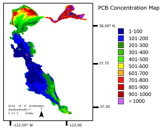
1. Introduction
Regarded for their strong chemical stability, high boiling point, and insulating properties, Polychlorinated biphenyls (PCBs) became ubiquitous in hundreds of different industrial and commercial applications throughout much of the 20th century, from insulators in electrical equipment to additives in oils, adhesives, and plastics [1]. During this time however, PCBs also became widely recognized as a threat to public health and the environment. In addition to their classification as a probable human carcinogen, PCBs are associated with a bevy of adverse health effects in humans, which include damage to the immune, reproductive, nervous, and endocrine systems [1,2,3,4,5]. Widespread concern over these adverse health risks prompted the U.S. Environmental Protection Agency (EPA) to ban the production of PCBs in 1979. However despite this nearly four decade-long production moratorium, PCBs, due in large part to their highly stable chemical structures, continue to persist in watersheds across the continental United States, often at concentrations considered hazardous to human health [2,3,6,7,8].
The San Francisco Bay (SFB) is characterized by a legacy of PCB contamination. Many industrial areas adjacent to the Bay exhibit high concentrations of PCBs and other contaminants that enter the SFB via urban runoff, outflow from the San Joaquin and Sacramento River delta, and erosion [9,10,11,12,13]. Once they have entered the SFB, PCBs, due to their non-polar molecular properties, accumulate in benthic sediments where they are periodically re-suspended in the water column, and transported by local currents [9,10,11,12,13]. As a result, PCBs are commonly found throughout the SFB at concentrations well above the Environmental Protection Agency’s (EPA) human health criterion (170 pg/L), and have been measured at concentrations ten times the threshold of concern for human health in the tissues of aquatic organisms [14]. The EPA classifies the SFB as an “impaired waterbody” under 303(d) listing criteria, which is due in large part to the Bay’s high concentrations of PCBs [15,16,17].
In order to ameliorate PCB contamination, the EPA has approved an action plan for the SFB, which includes a 10 kg/year total maximum daily load for PCBs [15,16,17]. However the successful implementation of any action plan pertaining to PCB remediation will require an effective PCB monitoring strategy. Such a strategy, according to the San Francisco Estuary Institute (SFEI) (Richmond, CA, USA), would identify areas of high susceptibility for PCB contamination within the SFB, and then closely monitor and track PCBs within these prioritized areas [14,18]. Nevertheless, PCB monitoring in the SFB is extremely limited in scope, due in large part to the nature of present-day (in situ) PCB sampling protocols, which are both expensive and laborious [14].
Remote sensing may offer a cost-effective and time saving alternative for in situ PCB monitoring in the SFB. Although PCBs cannot be remotely sensed directly, they are closely associated with sediments due to their affinity for non-polar substrates [9,10,11,12]. Suspended sediments in turn, can be detected via Earth-monitoring satellites. These satellites could, therefore, offer an indirect mechanism for estimating PCB concentration within the upper water column, providing that sediments are indeed a viable proxy for PCBs in the SFB [19,20,21,22]. In contrast with present-day in situ PCB measurements, which are only representative of the discrete locations and instances in time at which they are sampled, satellites offer the potential advantage of characterizing the spatial distribution of PCBs across the SFB. Furthermore, the availability of past satellite imagery could be leveraged to glean historical trends in PCB concentrations within the SFB.
This study examines the potential of using high spatial resolution satellite imagery to characterize the spatial distribution of PCBs within the SFB using a two-step empirical algorithm: step 1—derive SSC from satellite reflectance, and step 2—estimating PCBs from satellite-derived SSC. We carried this out by first establishing empirical relationships between PCB and SSC for the SFB, and then by gauging the relationships between in situ SSC and reflectance data from two Earth-monitoring satellites, the Landsat 8 Operational Land Imager (L8 OLI; 30 m resolution) and the Sentinel 2A Multi-Spectral Imager (S2-MSI; 10–60 m resolution), to determine whether sediment concentrations could be reliably estimated using imagery from different satellites. We also evaluated a “generic” SSC algorithm [20] using both >10 years of MODIS Aqua data and the L8 imagery. To further determine the robustness of the SSC-reflectance relationship in the SFB, we processed satellite imagery using several different atmospheric correction regimes. Finally, to demonstrate how this algorithm could be implemented to monitor PCBs throughout the SFB, we generated concentration maps of PCBs based on this two-step algorithm.
2. Materials and Methods
2.1. Study Area
SFB covers an area of 1240 km2. It is characterized by a mild Mediterranean climate with the majority of precipitation and riverine freshwater input occurring from late fall to early spring respectively [14,19,23,24]. Eighty-nine percent of variability in concentrations of suspended sediment is explained by tidal cycles, wind forcing, and riverine input, which vary markedly geographically across the bay, as well as seasonally [25]. For this reason the SFB is commonly divided into three sub-embayments with characteristic physical forcing: North Bay, Central Bay, and South Bay [19,23].
Residence time of water and, therefore, suspended sediment, varies between the North Bay, Central Bay, and South Bay, primarily as a result of differences in physical and climatological forcing. Sediment residence times for the North Bay, which vary seasonally on the order of days (winter) to over a month (summer), are driven primarily by seasonal fluctuations of freshwater inputs from the Sacramento and San Joaquin Rivers [23,24]. These two riverine sources, which account for 90% of the SFB’s freshwater inputs, transport large quantities of sediment from California’s Central Valley into the North Bay [26]. Suspended sediment in the North Bay is also influenced by spring and summer wind forcing, which re-suspends benthic sediments that have settled out of the water column, a process which dominates those seasons [27]. Of the three sub-embayments, the Central Bay exhibits the lowest concentrations of suspended sediment in the water column [27,28]. Due to its proximity to the mouth of the SFB, tidal forcing is the dominant hydrological process in the Central Bay [27]. Consequently, the Central Bay exhibits the lowest residence time, as a substantial portion of its water column (and its suspended sediments) is periodically flushed into the Pacific Ocean. Additionally, because the Central Bay is the deepest of the three sub-embayments, wind-driven re-suspension of benthic sediments is of a lesser influence than in the North and South Bay. The South Bay exhibits the highest concentrations of suspended sediments due to its high residence time, which can last for several months [29,30]. The South Bay receives only 10% of the estuary’s fresh water input, and is minimally flushed by tides [26]. Wind waves associated with flood tides (most common during the summer and fall seasons), as well as wind forcing, re-suspend benthic sediments in this sub-embayment [28].
For the purposes of these analyses, we partitioned the SFB into three sub-embayments, which we refer to as the Northern Bay, South-Central Bay, and Southern Bay, as their boundaries do not conform to the three established sub-embayments (referenced above). The Northern Bay comprises part of the Delta just north of Sherman Island to the Richmond San-Raphael Bridge. We define the South-Central Bay as spanning from the Richmond San-Raphael Bridge to the San Mateo Bridge. The Southern Bay is south of the San Mateo Bridge (Figure 1). The rationale for delineating these non-standard sub-embayments was two-fold: First, these regions match locations chosen by SFEI’s Regional Monitoring Program, which measured PCBs within these regions at discrete time intervals (Northern Bay—1998–2006, South-Central Bay—2002–2006, and Southern Bay—1998–2001). Second, suspended sediments and PCB concentrations exhibit significant statistical relationships within each of our three sub-embayments that are statistically distinct (p < 0.01), suggesting varying sources and fates of PCBs and sediments in these regions.
2.2. Data Collection
2.2.1. In Situ PCBs and Suspended Sediment
In situ measurements of total PCB concentration (PCBs) and suspended sediment concentration (SSC) were acquired from the SFEI’s Regional Monitoring Program [31]. A subset of these data, totaling 164 in situ water samples typically collected from February–August 1998 to 2006, was chosen for analysis. This subset represents available data points for which PCBs and SSC were measured at the same time and geographic location (Figure 1). All samples were collected at depths less than or equal to one meter. We also present more recent data but note that there are no recent contemporaneous PCB and sediment measurements.
PCBs (pg/L) were tabulated as the sum of 40 PCB target analyte concentrations analyzed in the water column. Prior to 2001, PCB analytes (pg/L) and SSC (mg/L) were analyzed using a gas chromatography/electron capture detector and SM-2540D, respectively. Beginning in 2001 these assays were performed using high resolution gas chromatography/mass spectrometry and ASTM D3977 respectively [32]. PCB analyses were changed to abide by EPA Method 1668A. For SSC, The primary difference between the methods is that SM-2540D is an analysis of an aliquot of the original water sample, while ASTM D3977 assays the entire sediment mass of the sample [33,34]. For subsequent analyses we make the assumption that these assays are directly comparable to each other, and therefore no correction was applied to the data.
2.2.2. Suspended Sediment Concentration and Satellite Imagery
To determine the feasibility of estimating SSC from satellite imagery, we used three satellite images collected on 27 June 2016, 13 July 2016, and 14 July 2016 for the SFB region. Satellite imagery from 27 June 2016 and 13 July 2016 was obtained from Landsat-8 (L8 OLI) [35]. Jointly operated by NASA and USGS, L8 is a low-orbiting satellite equipped with the Operational Land Imager, a push broom sensor that collects spectral bands at 30 m pixel resolution. L8 OLI imagery was atmospherically corrected using a standard terrestrial-based algorithm as well as the marine atmospheric correction software ACOLITE v. 20170718 (Royal Belgian Institute of Natural Sciences, Brussels, Belgium) [36,37]. With ACOLITE we performed both full and partial (Rayleigh) atmospheric corrections, yielding remote sensing reflectance (Rrs) and Rayleigh-corrected reflectance values (Rrc). Our reasoning for performing both full and Rayleigh atmospheric corrections were two-fold: 1. During analysis it was observed that ACOLITE is extremely sensitive to haze and cloud coverage, which can preclude a complete atmospheric correction, and 2. Because Rrs and Rrc are related, we wanted to evaluate the use of Rrc as an input to SSC estimates when Rrs is not available due to atmospheric correction failures. The 14 July 2016 image was obtained from the European Space Agency’s Sentinel 2A Multi-Spectral Imager (S2-MSI). Like L8 OLI, S2-MSI is a low orbiting push broom sensor. It collects spectral bands at 10–60 m resolution. S2-MSI imagery was atmospherically corrected using ACOLITE, with only Rrc retained for analysis due to a failure of Rrs for the majority of the images caused by haze and cloud.
These three satellite images were selected because they coincided (within ca. one day or less) with two cruises conducted in the SFB by the U.S. Geological Survey (USGS) (Menlo Park, CA, USA), for which SSC was sampled. Water samples were collected along a 145 km transect at 1 m depth at pre-determined sampling stations. SSC was determined gravimetrically using an aliquot of the water sample. The sample was vacuum filtered, dried, and weighed, as well as corrected for residual salt weight. We elected to use SSC data from USGS because there were no adequate satellite matchups with the aforementioned subset of SFEI data used to gauge the relationship between SSC and PCBs.
To assess the potential errors in estimating SSC using satellite imagery, we also used MODIS Aqua data from 2002 to 2015. While spatial resolution (1 km) is greatly reduced compared to S2 and L8, this was preferable given the significantly increased number of direct matchups. Data were extracted generally following [38]. Briefly, 3 × 3 Rrs (667 nm) pixels centered on USGS stations and within 24 h of field collection were extracted from MODIS L2 data acquired from the NASA Ocean Biology Processing Group. Data were filtered to remove matchups with less than 7 of 9 valid pixels, and within 3, 12, and 24 h of the field observations. The Rrs values were then used to calculate total suspended matter (TSM), comparable to SSC, following [20]. Both the median of nine pixels and the centroid pixel were used in the analysis; there were no significant differences for the full dataset, so subsequent analysis used the median value. The algorithm could not be applied to S2 imagery given the atmospheric correction issues.
We evaluated continuous (15 min) data from Central Bay (Angel Island) and South Bay (Dumbarton Bridge) for May 2016, collected by USGS (available at https://ca.water.usgs.gov/projects/baydelta/) to identify potential issues with temporal mismatch between satellite and field observations. Autocorrelations were calculated, and the first crossing point compared to 95% confidence intervals for a white noise process were considered the decorrelation scale.
2.3. Data Analysis
To gauge the feasibility of monitoring PCBs using spatially resolute satellite imagery two-step empirical relationships between PCBs and satellite reflectances (Rrs & Rrc) were developed. First, linear regression was used to compare SSC and PCBs. Here we compared SFEI-sampled SSC and PCBs across the SFB (n = 164), as well as within each of the three sub-embayments: Northern Bay (n = 90), South-Central Bay (n = 21), and Southern Bay (n = 53) (Figure 2; Table 1). Next, satellite reflectance (Rrs or Rrc) in the red (λ = 640–670 nm), previously shown to be a reliable proxy for sediment, was related to SSC [20,21]. We matched USGS-sampled in situ SSC with the corresponding red reflectance values from coincident satellite imagery. We then performed linear regression (Table 2). These steps were repeated for all four remote sensing products (satellite + atmospheric correction regime): terrestrial-derived Rrs from L8 OLI (n = 16), ACOLITE-derived Rrs from L8 OLI (n = 16), ACOLITE-derived Rrc from L8 OLI (n = 16), and ACOLITE-derived Rrc from S2 MSI (n = 5). Analysis of co-variance (ANCOVA) was performed to compare the localized linear relationships between SSC and PCBs between the three sub-embayments. Root mean square error (RMSE) was calculated to quantify the relationships between in situ PCB and SSC as well as satellite reflectance and SSC for all remote sensing products and sensors tested.
We indirectly examined the likelihood of the SSC to PCB relationship changing over time in San Francisco Bay. To ascertain this likelihood over the entire bay, we first combined the SFEI PCB data set (1998–2006) with more recent SFEI PCB measurements (2009–2011, 2016) based on the sum of 209 PCB analytes, and standardized the PCB residuals. The residuals were examined for temporal trends [38]. A similar analysis was performed for SSC using water quality data from the USGS shipboard time series [39]. These more recent PCB data (2009–2011, 2016) were excluded from our empirical algorithm (Table 1) because data do not contain spatially and temporally matching SSC. The discrepancy between the Sum of 40 and Sum of 209 PCBs is a result of the evolving analytical methods for PCBs (described above). However, comparison of the two show that sediment and organism PCB levels are highly correlated [40], and that the differing sums are also highly correlated in forage fish and we considered the two data sets therefore to be comparable [41].
3. Results
3.1. In Situ PCBs and Suspended Sediment
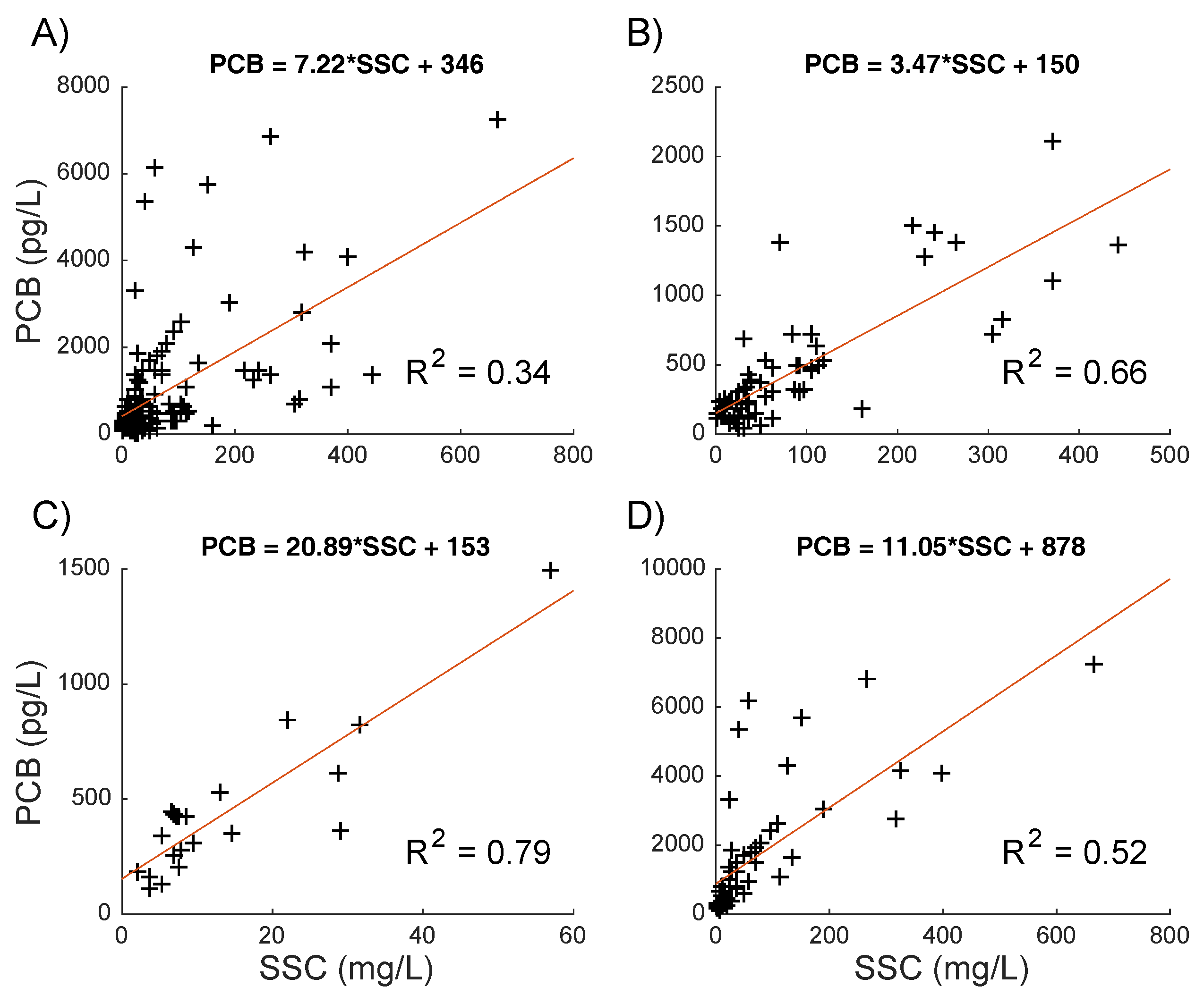
The relationship between SSC and PCBs across the SFB is significant, but weak (R2 = 0.28, p < 0.01). This relationship improves substantially (R2 > 0.5, p < 0.01) when linear regressions are localized to the three sub-embayments (Table 1; Figure 2). ANCOVA indicates that the relationships between SSC and PCBs differ significantly across the three sub-embayments (p < 0.01). Since the SFB exhibits strong regional differences in residence times, riverine inputs, tidal forcing, and currents, we would expect that the relationship between SSC and PCBs would differ across the three sub-embayments. RMSE and percent mean error also indicate the existence of a strong relationship between SSC and PCBs.
3.2. Suspended Sediment and Satellite Imagery
Strong relationships between red reflectance and SSC were observed for all four remote sensing products (R2 > 0.72, p < 0.01; Table 2). The strength of these correlations suggests that the relationship between red reflectance and SSC is extremely robust, and can be reliably estimated using imagery generated from a multitude of remote sensing products. RMSE was relatively high across the four relationships (1.44–2.67 mg/L) (Table 2; converted from log-space). To directly compare results by sub-embayment, RMSE from Table 2 was converted to a percentile range for the various algorithms and methods. The South-Central Bay exhibits a disproportionately high amount of the error (RMSE = 69–78%) relative to Southern Bay (RMSE = 39–40%). The Northern Bay’s small sample size precluded percent estimates of RMSE.
3.3. Total Error for PCB Estimates
Given the two-step algorithm, total error results from a combination of the satellite-derived SSC values and the conversion of SSC to PCB. In this analysis the error is driven by the SSC determination which exhibits up to 48% error, resulting in total error of ~60%. We note, however, that if data are restricted to times when the TSM relationship of Nechad et al. (2010) [20] can be used, the total error would be between 35% and 60%, with improvements when using tighter spatial and temporal matchup criteria.
4. Discussion
4.1. In Situ Measurements and Satellite Imagery
The strong relationship between SSC and PCBs, as indicated by linear regression and RMSE, suggest that the primary limitation in application of this proposed method is the remote detection of SSC [42]. Similarly, application of this method beyond SFB would require measurements of local SSC and PCB concentrations. This could facilitate regional understandings of the relationship between SSC and PCBs, which could then be used to account for the spatial and temporal variability of PCBs within those regions.
With regards to red reflectance vs. SSC, the higher RMSE observed in the South-Central Bay compared to the Southern Bay can be explained by the fact that the South-Central Bay is subject to significantly more tidal forcing than either the Northern Bay or Southern Bay. It would, therefore, be expected that SSC would fluctuate more rapidly diurnally in the South-Central Bay than either of the other two sub-embayments due to its low residence time [27,28,29,30]. Consequently, the South-Central Bay would be more sensitive to the temporal mismatches between satellite imagery and USGS cruises relative to the Northern Bay and Southern Bay.
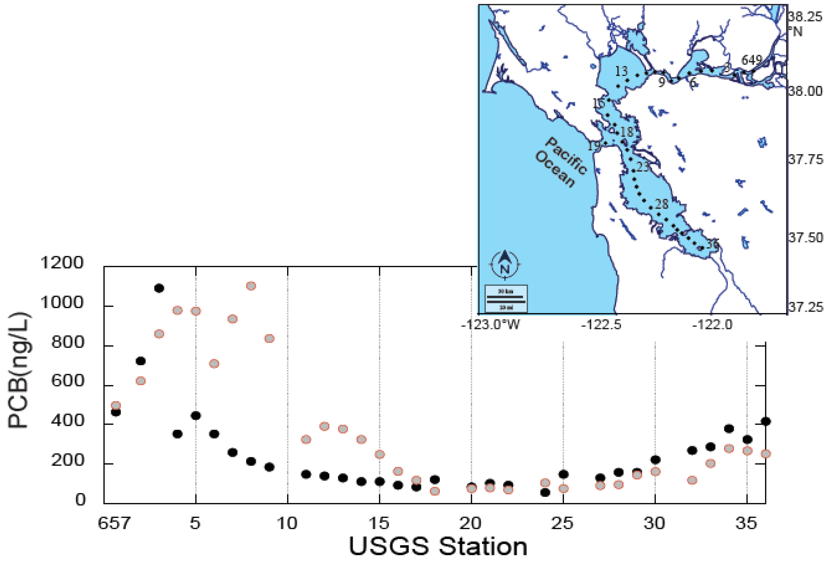
It should be noted that these findings are not without potential sources of error. The sample size in these analyses (particularly for Sentinel 2A) was limited by the availability adequate spatial and temporal (time < 24 h) matchups between in situ SSC measurements and satellite reflectances. It should also be noted that L8 OLI imagery was sampled ca. one day prior to USGS cruises (L8 OLI imagery: 06/27/2016, 07/13/2016; USGS in situ measurements: 06/28/2016, 07/14/2016). This is a potential source of error, as SSC would be expected to change during this intervening time due to hydrological forcings (e.g., tides, currents, and fluvial influx), which can alter the spatial distribution of suspended sediments over relatively short timescales (<1 day) [43]. Intuitively, the existence significant time lag between SSC and reflectance would be expected to degrade and not improve the reflectance/SSC relationship. Indeed this is what we observed. Evidenced by Figure 3, SSC varied markedly between USGS cruises and L8 OLI across USGS cruise stations north of the mouth of the SFB. Improved agreement at stations south of the mouth may be attributed, at least in part, to higher residence times, which characterize the South Bay [29]. The satellite data were collected during a rising tide, while stations 1–15 were collected (offset by eight days) on a falling tide, while the remaining stations were during a rising tide (tidal magnitude was very similar for the two days). Analysis of continuous (15 min) data from sites in the South Bay (Dumbarton Bridge) and Central Bay (Angel Island) also showed autocorrelation for ~3–4 h, with repeating (tidal) correlations extending for ca. four days in the Central Bay, but ~7–8 days in the South Bay.
Nevertheless, a strong overall relationship between L8 OLI red reflectance and SSC was still observed (R2 = 0.73–0.77, p < 0.01). This attests to the strength and robustness of the reflectance/SSC relationship, as we would expect the correlation between SSC and reflectance to have been higher, had L8 OLI imagery and SSC been sampled simultaneously. The improved relationship and lower error between SSC and red reflectance generated using Sentinel 2A imagery (Table 2), buttresses this assumption, as these data were collected on the same day, hours apart.
The strong relationships that we have observed between red reflectance and suspended sediments are also consistent with previous studies [19,20,21]. Using AVHRR satellite sensors [19] demonstrate similar relationships between SSC and reflectance in the SFB to the ones that we observed (R2 = 0.59, RMSE = 0.17). Moreover, [20] also report strong relationships in the North Sea between TSM and reflectance (650–750 nm) derived from three distinct Earth-monitoring satellites: MERIS, MODIS, and SeaWiFS (R2 = 0.79–0.93, error = 30–40%). These studies further demonstrate the robustness of the SSC vs. reflectance relationship with respect to remote sensing products, as well as geographic location.
4.2. PCB Concentration Maps
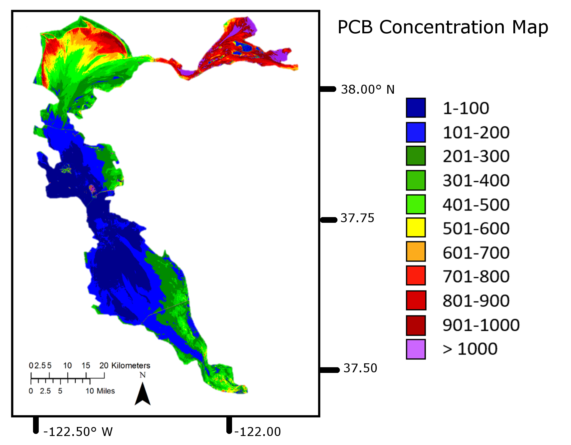
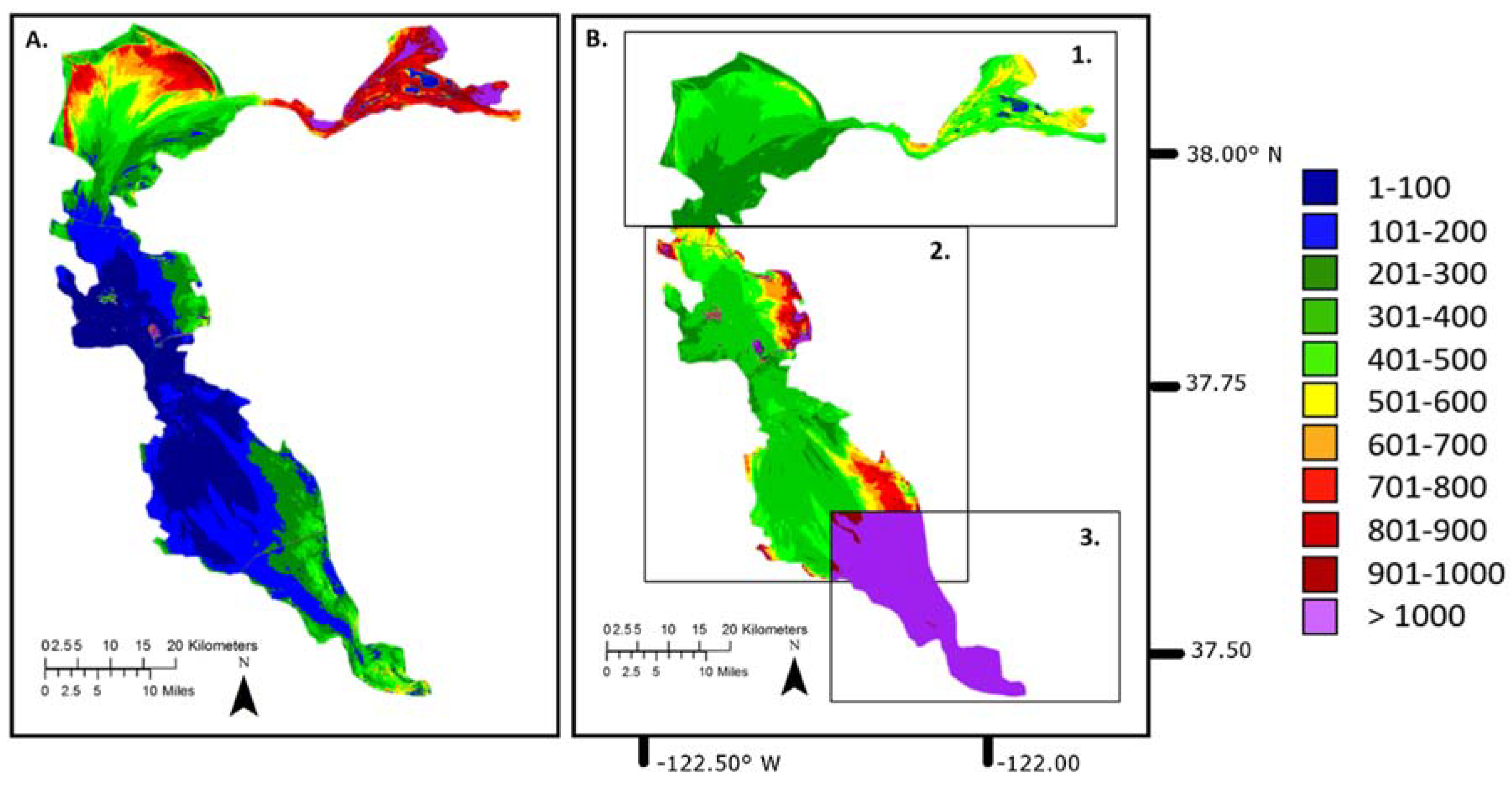
To demonstrate the potential utility of our proposed two-step empirical algorithm in estimating PCBs in the SFB, we produced two PCB concentration maps using the L8 OLI image, sampled on 26 May 2016 and corrected using OLI’s terrestrial-based algorithm (Figure 4). The first map (Figure 4A) uses a modified empirical SSC to PCB relationship derived for the entire SFB, while the second (Figure 4B) uses localized relationships specific to each sub-embayment (see Figure 1). Each of these approaches offer distinct advantages. Mapping PCBs using the SSC to PCBs relationship fitted for the entire SFB (Figure 4A) provides a continuous estimate of surface concentrations for the entire SFB with no arbitrary boundaries. However, this approach sacrifices accuracy, as localized SSC to PCBs relationships were statistically more robust (Figure 2; Table 1). Additionally, because an estimated 99.8% of PCBs are particulate in nature (bound to sediment) [44,45], PCBs are not detectable in the water column in the absence of suspended sediment. To enforce this observation, the y-intercept of the SSC to PCB was forced through zero for Figure 4A (see Table 1). Alternatively, building concentration maps using SSC to PCBs relationships localized to the three sub-embayments (Figure 4B) substantially improves the accuracy of the concentration map. However, when using the localized relationships, sub-embayments must be defined geographically. This leads to discontinuous concentration gradients, separated by artificial geographical boundaries between the sub-embayments. While we continue to acknowledge that PCBs likely drop to zero in the absence of suspended sediment, we did not force y-intercepts through zero for localized SSC to PCB relationships. Our reasoning behind this was that these relationships are substantially stronger (and more accurate) than the SSC to PCB for the entire SFB. Forcing these localized y-intercepts through zero is therefore likely to degrade the accuracy and predictive capacity of Figure 4B. It would also diminish the agreement between Figure 4A,B. Here we should point out that it was the forcing the y-intercept of the entire SFB SSC to PCB relationship to zero that maximized agreement between Figure 4A,B (and likely the accuracy of Figure 4A as well).
Concentration maps produced using satellite imagery offer great promise as a method for higher spatial and temporal resolution PCB monitoring. While PCB concentration maps, the finished product of our efforts, are less accurate than in situ sampling, they provide a view of the relative spatial distribution of PCBs in SFB. Given that PCB concentrations in the SFB have consistently exceeded proposed total daily maximum load (TMDL) values by orders of magnitude [14], the ~60% RMSE error documented in this study suggest that a remote-sensing approach for estimating spatial/temporal concentrations of PCBs would be useful for management purposes. Producing series of these maps from sequential satellite images would enable spatial distribution of PCBs to be tracked through time. This far exceeds the scope of in situ data, which although more accurate, are constrained to specific times and places where sampled. Our maps also demonstrate that PCB concentrations can vary markedly across the SFB (Figure 4 and Figure 5); SFEI sampling stations may not be representative of areas in close proximity (Figure 4 and Figure 5). More accurate PCB concentration maps depend on improved understanding of regional SSC vs. PCB relationships and their spatial and geographic constraints. More consistent in situ monitoring would also improve understanding of hydrological and meteorological forcing and would validate the remote sensing approach. As our data was collected predominantly during the dry season, we cannot be certain as to whether our empirically-derived SSC vs. PCB relationships differ during the rainy season. Filling in these gaps will require more rigorous and consistent PCB and SSC monitoring throughout the SFB.
4.3. Limitations of Our Two-Step Algorithm
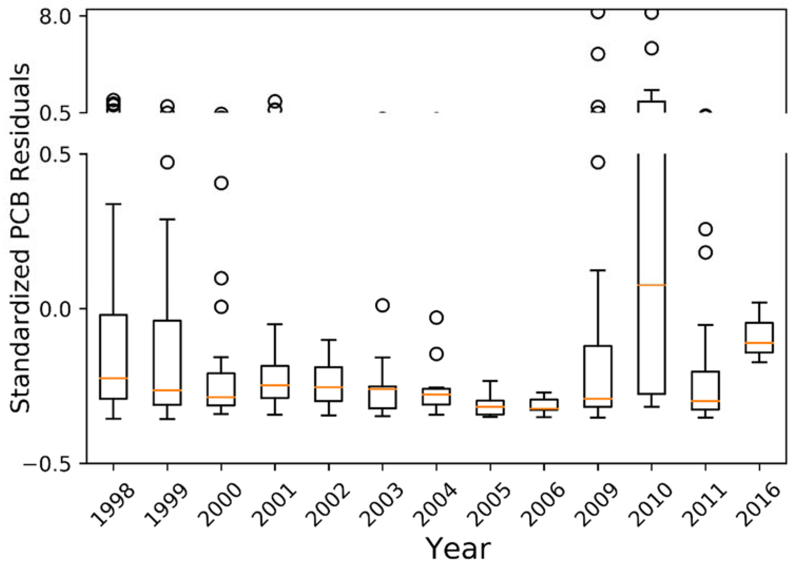
The PCB concentration maps (Figure 4) generated in this study rely on two underlying assumptions: first, that the relationship between PCBs and sediment remain consistent over time, and second, that suspended sediments at the water surface are representative of the entire water column. We base our first assumption on the fact that PCB hydrophobicity and long half life result in a strong association with sediments, where they are likely to remain for many years [42,46]. The concept that PCB concentration remains stable, despite the 40-year production moratorium, is well documented. For instance, PCB tissue concentrations have remained relatively consistent in shiner perch across the SFB over a 20-year period (1994–2014) [47]. Shiner perch are considered an indicator species for assessing PCB total maximum daily load and, hence, reflects ambient SFB PCB concentrations [48]. These findings are bolstered by [18], who demonstrate a strong linear relationship between PCB in sediment and PCB in fish tissue, and report that local PCB concentrations remain stable over time. Our statistical analysis of PCB trends through time support this with no significant trend identified (p > 0.5) (Figure 6). Although the availability of coinciding PCB and SSC are limited, we also point out that, in the Northern Bay, the empirical relationship between SSC and PCBs did not change over time, as tested by ANCOVA (p > 0.75) (1998–2001: y = 3.511x + 153, R2 = 0.66; 2002–2006: y = 3.281x + 149, R2 = 0.50). We, therefore, assume that PCB/SSC relationships observed from 1998 to 2006 are still applicable today, within the associated error of our model, and can be used with current satellite imagery.
The veracity of our second assumption, that suspended sediments at the water surface are representative of the entire water column, is supported by previous observations. According to [14], the most effective indicator of the spatial distribution of PCB impairment in the SFB is by PCB concentrations in surface (benthic) sediments. However, the SFB is shallow over the shoals, with an average depth of 5.3 m, and a median depth of 2 m [45]. The shallow depth of the SFB combined with strong wind- and tide-driven currents result in an intense mixing of sediment, with large rates of resuspension and deposition. Subsequently, a high rate of exchange exists between particles of water and sediment in the SFB, resulting in elevated SSC in the water column [45]. In a one-box model observing the long-term fate of PCBs in the SFB, water and sediment are so tightly coupled by this rate of exchange that they are assumed to effectively behave as one compartment [45,49]. Additional studies examining regions of the SFB have shown that the estuary is generally considered to be weakly stratified and typically mixed, excluding specific conditions, such as seasonal high fresh water flow or climatological anomalies which temporarily suppress mixing [50,51]. However, we do acknowledge that the shipping channels and Central Bay (proper) are significantly deeper than the shoals (~15 m), and our method would only capture the trends and patterns in the upper well-mixed water column.
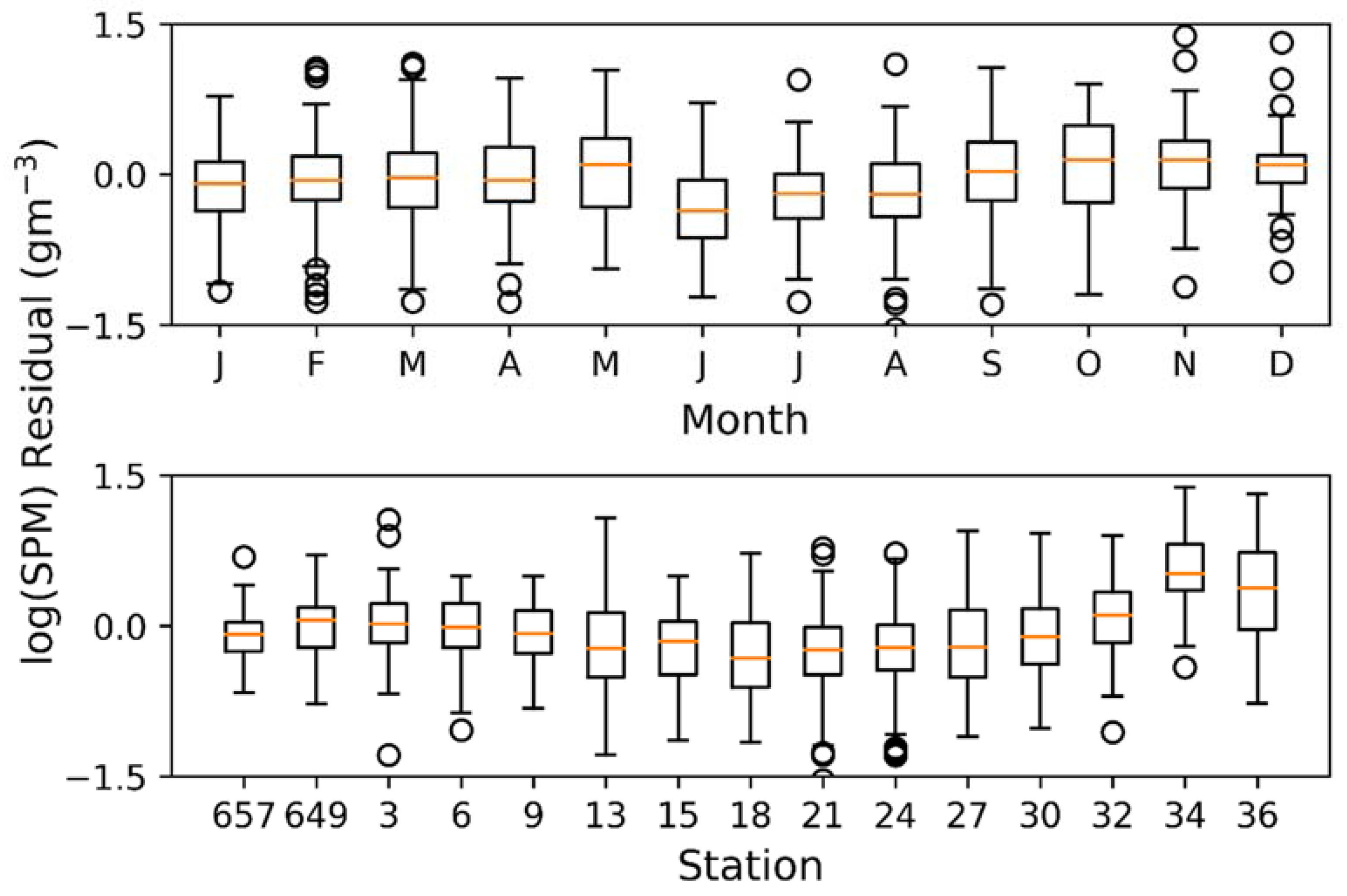
To assess whether estimates of SSC (TSM) are robust for San Francisco Bay we also evaluated MODIS AQUA data from 2002 to 2015. For the full dataset (n = 1200), the algorithm performed as expected based on [20] with RMSE of 5.12 mg m−3 and 55% error. Reducing the matchups to 12 (n = 949) and 3 (n = 778) h resulted in RMSE of 5.08 and 2.89 mg m−3, with 55% and 36% error, respectively. For comparison, errors for MODIS of 10.98 mg m−3, or 37%, were reported (Table 10 [20]). The 3 h matchup data were subsequently used to generate residual errors between observations and MODIS by month and by station. The satellite estimates were consistently lower during June, July, and August (i.e., when fog and haze are common in the region), but there were no other strong spatial or temporal patterns in the residual errors (Figure 7), suggesting that, as expected, robust estimates of SSC can be obtained from satellite observations for this region. For the analysis of S2 and L8, the atmospheric correction frequently failed, leading us to develop local empirical relationships for imagery. For the L8 data there were enough full retrievals (n = 16) to apply the [20] method, as well, with good results (Table 2).
5. Conclusions
In this study we demonstrate the feasibility of estimating polychlorinated biphenyls (PCBs) from red reflectance in the San Francisco Bay (SFB) using a two-step empirical algorithm. We demonstrate strong relationships between in situ suspended sediment concentration (SSC) and PCBs in all three SFB sub-embayments (R2 > 0.5, p < 0.01), as well as a robust relationship between SSC and satellite measurements for both Landsat 8 and Sentinel 2A (R2 > 0.72, p < 0.01). Total error (~60%) results from a combination of the satellite-derived SSC values and the conversion of SSC to PCB, with error in this analysis driven by SSC determination (up to 48%). This study is limited by, and could be improved with, the addition of data for both in situ measurements of SSC and PCBs, as well as satellite imagery that corresponds with in situ sampling. In situ PCB and SSC measurements used in this study were collected by the San Francisco Estuary Institute (SFEI) in February, April, July, and August from 1998–2006 (n = 164) at locations throughout the SFB (Northern Bay data collected in February, April, July, August, 1998–2006; South-Central Bay data collected in July, August, 2002–2006; Southern Bay data collected in February, April, July, August, 1998–2001). Satellite imagery (n = 16) used in this study were sampled ca. one day prior to in situ SSC measurements, with the exception of the S2-MSI image (n = 5) (L8 OLI imagery: 06/27/2016, 07/13/2016; USGS in situ measurements: 06/28/2016, 07/14/2016. S2-MSI image: 07/14/2016; USGS in situ measurements: 07/14/2016). The data in this study are therefore limited by the availability of adequate matchups between in situ measurements of SSC and PCBs (1998–2006), time of the year in situ SSC and PCBs were collected (primarily the dry season), as well as corresponding satellite images and in situ SSC measurements. The accuracy and error of our empirical algorithm, therefore, could be better validated by increased in situ measurements of SSC and PCBs, as well as tighter spatial and temporal matchup criteria for satellite imagery. While analysis of in situ PCB and SSC concurrent with the satellite observations suggests that the relationships used in our models are still valid, we cannot rule out the possibility, without recent simultaneous estimates of PCB and SSC, that the relationship has changed. Despite these data limitations, our results indicate that the empirical algorithm could be used with imagery collected using a diverse array of Earth-monitoring satellites and processed using multiple atmospheric correction methods with consistent and reliable results. One of the primary strengths of our two-step algorithm is that it can be employed to generate concentration maps of PCBs in any water body sampled by satellites, if there are sufficient data to develop a regional relationship between SSC and PCBs. Furthermore, because satellites typically sample locations (e.g., the SFB) at consistent time intervals, this algorithm could be used to track PCBs within a given water body over time. It would enable the implementation of SFEI’s recommendations of identifying high-priority areas for PCB monitoring in the SFB. Stakeholders could then concentrate their finite resources, such as in situ sampling of SSC and PCBs in these areas, which would in turn improve our ability to remotely sense PCBs in the SFB, especially if sampling was carried out in conjunction with satellite flybys. These efforts may also lead to increased understanding of the roles of seasonality, precipitation, erosion events, and tidal forcing on spatial distributions PCBs [14,19].
Author Contributions
A.E.H. and J.T.B. conceived and designed the study, under the auspices of R.M.K.; A.E.H. selected and retrieved the publically accessible data and performed all quantitative analyses, including in situ analysis and satellite imagery analysis, and the generation of PCB concentration maps under the direct supervision of J.T.B.; and A.E.H. and J.T.B. co-wrote the paper, with significant contributions from R.M.K., who played a prominent and vital role in editing and revising the paper. All authors created figures for the paper.
Acknowledgments
This work was performed with the National Aeronautics and Space Administration Student Airborne Research Program (NASA SARP). We thank Emily Schaller (NASA SARP), Niky Taylor (NASA SARP), Nick Wiesenberg (College of Wooster), and Greg Wiles (College of Wooster) for their help and contributions. Comments from three anonymous reviewers greatly improved the manuscript. We also thank the SFEI Regional Monitoring Program and U.S. Geological Survey. This publication was partially supported by the NASA Student Airborne Research Program and by NASA award NNX12AQ23G through the HyspIRI Airborne Campaign for data analysis and synthesis. NASA requires public access for all data and products supported by NASA funding, including Open Access for peer-reviewed publications, and the authors adhere to these guidelines. This study is dedicated in loving memory of Melissa M. Schultz, College of Wooster.
Conflicts of Interest
The authors declare no conflict of interest. The funding sponsors had no role in the design of the study; in the collection, analyses, or interpretation of data; in the writing of the manuscript; or in the decision to publish the results.
References
- Learn about Polychlorinated Biphenyls (PCBs), US Environmental Protection Agency, 2016. Available online: https://www.epa.gov/pcbs/learn-about-polychlorinated-biphenyls-pcbs (accessed on 8 November 2016).
- Abramowicz, D.A. Aerobic and anaerobic biodegradation of PCBs: A review. Crit. Rev. Biotechnol. 1990, 10, 241–251. [Google Scholar] [CrossRef]
- Safe, S.H. Polychlorinated biphenyls (PCBs), Dibenzo-p-Dioxins (PCDDs), Dibenzofurans (PCDFs), and related compounds: environmental and mechanistic considerations which support the development of toxic equivalency factors (TEFs). Crit. Rev. Toxicol. 1990, 21, 51–88. [Google Scholar] [CrossRef] [PubMed]
- Safe, S.H. Polychlorinated biphenyls (PCBs): Environmental impact, biochemical and toxic responses, and implications for risk assessment. Crit. Rev. Toxicol. 1994, 24, 87–149. [Google Scholar] [CrossRef] [PubMed]
- Gunther, A.J.; Davis, J.A.; Hardin, D.D.; Gold, J.; Bell, D.; Crick, J.R.; Scelfos, G.M.; Sericano, J.; Stephenson, M. Long-term bioaccumulation monitoring with transplanted bivalves in the San Francisco Estuary. Mar. Pollut. Bull. 1999, 38, 170–181. [Google Scholar] [CrossRef]
- Cogliano, V.J. Assessing the cancer risk from environmental PCBs. Environ. Health Perspect. 1998, 106, 317–323. [Google Scholar] [CrossRef] [PubMed]
- Baan, R.; Grosse, Y.; Straif, K.; Secretan, B.; El Ghissassi, F.; Bouvard, V.; Benbrahim-Tallaa, L.; Guha, N.; Freeman, C.; Galichet, L.; Cogliano, V. A review of human carcinogens—Part F: Chemical agents and related occupations. Lancet Oncol. 2009, 10, 1143–1144. [Google Scholar] [CrossRef]
- Hopf, N.B.; Ruder, A.M.; Succop, P.; Waters, M.A. Evaluation of cumulative PCB exposure estimated by a job exposure matrix versus PCB serum concentrations. Environ. Sci. Pollut. Res. 2014, 21, 6314–6323. [Google Scholar] [CrossRef] [PubMed]
- Kuwabara, J.S.; Chang, C.C.Y.; Cloern, J.E.; Fries, T.L.; Davis, J.A.; Luoma, S.N. Trace metal associations in the water column of South San Francisco Bay, California. Estuar. Coast. Shelf Sci. 1989, 28, 307–325. [Google Scholar] [CrossRef]
- Domagalski, J.L.; Kuivila, K.M. Distributions of pesticides and organic contaminants between water and suspended sediment, San Francisco Bay, California. Estuaries 1993, 16, 416–426. [Google Scholar] [CrossRef]
- Flegal, A.R.; Rivera-Duarte, I.; Ritson, P.I.; Scelfo, G.; Smith, G.J.; Gordon, M.; Sanudo-Wilhelmy, S.A. Metal contamination in San Francisco Bay waters-historic perturbations, contemporary concentrations, and future considerations. In San Francisco Bay—The Ecosystem; Hollibaugh, J.T., Ed.; Pacific Division of the American Association for the Advancement of Science: San Francisco, CA, USA, 1996; pp. 173–188. [Google Scholar]
- Schoellhamer, D.H.; Wright, S.A.; Drexler, J.Z. Conceptual model of sedimentation in the Sacramento—San Joaquin River Delta. San Franc. Estuary Watershed Sci. 2012, 10, 2–25. [Google Scholar]
- Oros, D.R.; Hoover, D.; Rodigari, F.; Crane, D.; Sericano, J. Levels and distribution of Polybrominated diphenyl ethers in water, surface sediments, and bivalves from the San Francisco Estuary. Environ. Sci. Technol. 2005, 39, 33–41. [Google Scholar] [CrossRef] [PubMed]
- Davis, J.A.; Hetzel, F.; Oram, J.J.; McKee, L.J. Polychlorinated biphenyls (PCBs) in San Francisco Bay. Environ. Res. 2007, 105, 67–86. [Google Scholar] [CrossRef] [PubMed]
- Evaluation of Water Quality Conditions for the San Francisco Bay Region; 303(d) List Revisions; 303(d) List; California Water Boards (SFBRWQCB): San Francisco, CA, USA, 2009. Available online: http://www.waterboards.ca.gov/rwqcb2/board_decisions/adopted_orders/2009/R2-2009-0008.pdf (accessed on 8 July 2016).
- Water Quality Standards; Establishment of Numeric Criteria for Priority Toxic Pollutants for the State of California, 40 CFR Part 131.38; United States Environmental Protection Agency: Washington, DC, USA, 2000.
- Total Maximum Daily Load (TMDL) Program. Available online: https://www.waterboards.ca.gov/water_issues/programs/tmdl/ (accessed on 16 January 2017).
- Davis, J.A.; McKee, L.J.; Jabusch, T.; Yee, D.; Ross, J.R.M. PCBs in San Francisco Bay: Assessment of the Current State of Knowledge and Priority Information Gaps. In RMP Contribution; No. 727; San Francisco Estuary Institute: Richmond, CA, USA, 2014. [Google Scholar]
- Ruhl, C.A.; Schoellhamer, D.H.; Stumpf, R.P.; Lindsay, C.L. Combined use of remote sensing and continuous monitoring to analyze the variability of suspended-sediment concentrations in San Francisco Bay, California. Estuar. Coast. Shelf Sci. 2001, 53, 801–812. [Google Scholar] [CrossRef]
- Nechad, B.; Ruddick, K.G.; Park, Y. Calibration and validation of a generic multisensory algorithm for mapping of total suspended matter in turbid waters. Remote Sens. Environ. 2010, 114, 854–866. [Google Scholar] [CrossRef]
- Aurin, D.; Mannino, A.; Franz, B. Spatially resolving ocean color and sediment dispersion in river plumes, coastal systems, and continental shelf waters. Remote Sens. Environ. 2013, 137, 212–225. [Google Scholar] [CrossRef]
- Fichot, C.G.; Downing, B.D.; Bergamaschi, B.A.; Windham-Myers, L.; Marvin-DiPasquale, M.; Thompson, D.R.; Gierach, M.M. High-resolution remote sensing of water quality in the San Francisco Bay–Delta Estuary. Environ. Sci. Technol. 2016, 50, 573–583. [Google Scholar] [CrossRef] [PubMed]
- Benoit, M.D.; Kudela, R.M.; Flegal, A.R. Modeled trace element concentrations and partitioning in the San Francisco Estuary, based on suspended solids concentration. Environ. Sci. Technol. 2010, 44, 5956–5963. [Google Scholar] [CrossRef] [PubMed]
- Smith, L.H. A Review of Circulation and Mixing Studies of San Francisco Bay, California; U.S. Geological Survey Circular 1015; U.S. Geological Survey: Reston, VA, USA, 1987.
- Schoellhamer, D.H. Variability of suspended-sediment concentration at tidal to annual time scales in San Francisco Bay, USA. Cont. Shelf Res. 2002, 22, 1857–1866. [Google Scholar] [CrossRef]
- Barnard, P.L.; Schoellhamer, D.H.; Jaffe, B.E.; McKee, L.J. Sediment transport in the San Francisco Bay Coastal System: An overview. Mar. Geol. 2013, 345, 3–17. [Google Scholar] [CrossRef]
- Lacy, J.R.; Schoellhamer, D.H.; Burau, J.R. Suspended-solids flux at a shallow-water site in South San Francisco Bay, California. In Proceedings of the North American Water and Environment Congress, Anaheim, CA, USA, 24–28 June 1996. [Google Scholar]
- Walters, R.A.; Cheng, R.T.; Conomos, T.J. Time scales of circulation and mixing processes of San Francisco Bay waters. In Temporal Dynamics of an Estuary: San Francisco Bay; Cloern, J.E., Nichols, F.H., Eds.; Springer: Dordrecht, The Netherlands, 1985; Volume 30, pp. 13–36. ISBN 978-94-009-5528-8. [Google Scholar]
- Schoellhamer, D.H. Sudden clearing of estuarine waters upon crossing the threshold from transport to supply regulation of sediment transport as an erodible sediment pool is depleted: San Francisco Bay, 1999. Estuaries Coasts 2011, 34, 885–899. [Google Scholar] [CrossRef]
- Gray, J.R.; Glysson, G.D.; Turcios, L.M.; Schwarz, G.E. Comparability of Suspended-Sediment Concentration and Total Suspended Solids Data; U.S. Geological Survey Water-Resources Investigations Report 00-4191; U.S. Geological Survey: Reston, VA, USA, 2000; pp. 3–4.
- Regional Monitoring Program (RMP) for Water Quality in San Francisco Bay. Available online: http://sfei.org/rmp (accessed on 16 January 2017).
- Wong, A.; Data Services, San Francisco Estuary Institute, San Francisco, CA, USA. Personal communication, February 2017.
- Glysson, G.D.; Gray, J.R.; Conge, L.M. Adjustment of Total Suspended Solids Data for Use in Sediment Studies. In Proceedings of the ASCE’s 2000 Joint Conference on Water Resources Engineering and Water Resources Planning and Management, Minneapolis, MN, USA, 30 July–2 August 2000; U.S. Geological Survey: Reston, VA, USA, 2000; p. 10. [Google Scholar]
- USGS Earth Explorer. Landsat Archive: Landsat Surface Reflectance-L8 OLI/TIRS. Database. 2016. Available online: http://earthexplorer.usgs.gov/ (accessed on 28 June 2016).
- Vanhellemont, Q.; Ruddick, K. Turbid wakes associated with offshore wind turbines observed with Landsat 8. Remote Sens. Environ. 2014, 145, 105–115. [Google Scholar] [CrossRef]
- Vanhellemont, Q.; Ruddick, K. Advantages of high quality SWIR bands for ocean colour processing: Examples from Landsat-8. Remote Sens. Environ. 2015, 161, 89–106. [Google Scholar] [CrossRef]
- Zhou, X.; Marani, M.; Albertson, J.D.; Silvestri, S. Hyperspectral and multispectral retrieval of suspended sediment in shallow coastal waters using semi-analytical and empirical methods. Remote Sens. 2017, 9, 393. [Google Scholar] [CrossRef]
- Kahru, M.; Kudela, R.M.; Manzano-Sarabia, M.; Mitchell, B.G. Trends in the surface chlorophyll of the California Current: Merging data from multiple ocean color satellites. Deep-Sea Res. II 2012, 77–80, 89–98. [Google Scholar] [CrossRef]
- Schraga, T.S.; Nejad, E.S.; Martin, C.A.; Cloern, J.E. USGS Measurements of Water Quality in San Francisco Bay (CA), Beginning in 2016; U.S. Geological Survey Data Release: Reston, VA, USA, 2018.
- Davis, J.A.; Yee, D.; Gilbreath, A.N.; McKee, L.J. Conceptual Model to Support PCB Management and Monitoring in the Emeryville Crescent Priority Margin Unit; SFEI Contribution #824; San Francisco Estuary Institute: Richmond, CA, USA, 2017. [Google Scholar]
- Greenfield, B.K.; Allen, R.M. Polychlorinated biphenyl spatial patterns in San Francisco Bay forage fish. Chemosphere 2013, 90, 1693–1703. [Google Scholar] [CrossRef] [PubMed]
- Montelay-Massei, A.; Ollivon, D.; Garban, B.; Teil, M.J.; Blanchard, M.; Chevreuil, M. Distribution and spatial trends of PAHs and PCBs in soils in the Seine River basin, France. Chemosphere 2003, 55, 555–565. [Google Scholar] [CrossRef] [PubMed]
- McKee, L.J.; Ganju, N.K.; Schoellhamer, D.H. Estimates of suspended sediment entering San Francisco Bay from the Sacramento and San Joaquin Delta, San Francisco Bay, California. Hydrology 2006, 323, 335–352. [Google Scholar] [CrossRef]
- SFEI. 2015 Annual Monitoring Report. The Regional Monitoring Program for Water Quality in the San Francisco Bay (RMP); Contribution #775; San Francisco Estuary Institute: Richmond, CA, USA, 2016. [Google Scholar]
- Davis, J. Long-term fate of Polychlorinated Biphenyls in San Francisco Bay (USA). Environ. Toxicol. Chem. 2004, 23, 2396–2409. [Google Scholar] [CrossRef] [PubMed]
- Sinkkonen, S.; Paasivirta, J. Degradation half-life times of PCDDs, PCDFs, and PCBs for environmental fate modeling. Chemosphere 2000, 40, 943–949. [Google Scholar] [CrossRef]
- Sun, J.; Davis, J.A.; Bezalel, S.N.; Ross, J.R.M.; Wong, A.; Yee, D.; Fairey, R.; Bonnema, A.; Crane, D.B.; Grace, R.; et al. Contaminant Concentrations in Fish from San Francisco Bay, 2014. Regional Monitoring Program for Water Quality in San Francisco Bay (RMP); SFEI Contribution #806; San Francisco Estuary Institute: Richmond, CA, USA, 2017. [Google Scholar]
- SFBRWQCB. Total Maximum Daily Load for PCBs in San Francisco Bay: Staff Report for proposed Basin Plan Amendment; San Francisco Regional Water Quality Control Board: Oakland, CA, USA, 2008.
- Connolly, J.P.; Ziegler, C.K.; Lamoureux, E.M.; Benaman, J.A.; Opdyke, D. Comment on “the long-term fate of Polychlorinated biphenyls in San Francisco bay, (USA)”. Environ. Toxicol. Chem. 2005, 24, 2397–2398. [Google Scholar] [CrossRef] [PubMed]
- Wilkerson, F.P.; Dugdale, R.C.; Hogue, V.E.; Marchi, A. Phytoplankton blooms and nitrogen productivity in San Francisco Bay. Estuaries 2006, 29, 401–416. [Google Scholar] [CrossRef]
- Cloern, J.E.; Schraga, T.S.; Lopez, C.B.; Knowles, N. Climate anomalies generate an exceptional dinoflagellate bloom in San Francisco Bay. Geophys. Res. Lett. 2005, 32, L14608. [Google Scholar] [CrossRef]
Figure 1.
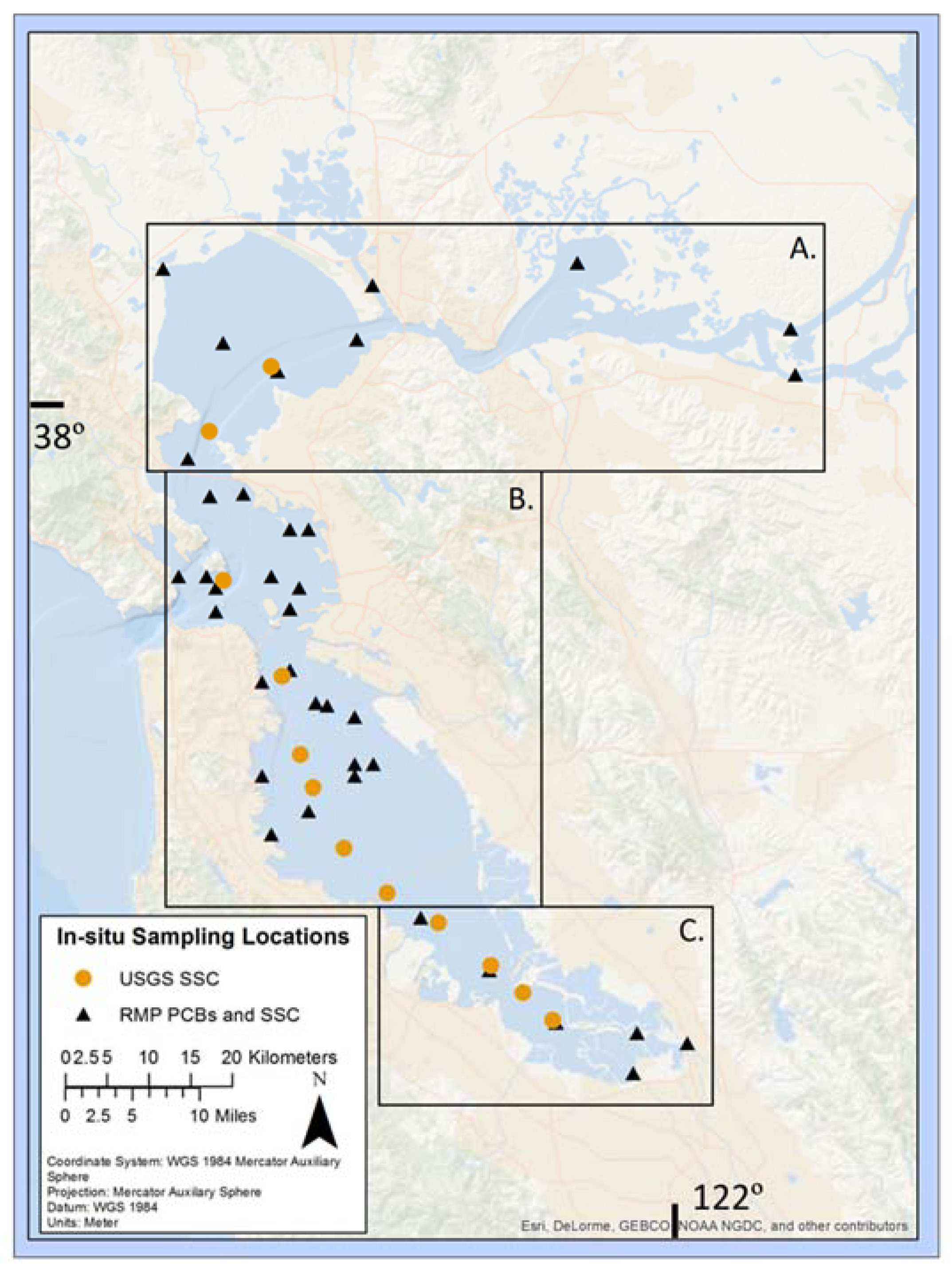
San Francisco Bay sampling locations; 1998–2006 PCB/SSC, 2016 SSC/reflectance. Boxes indicate the following sub-embayments: A. Northern Bay (San Pablo and Suisun Bays); B. South-Central Bay; and C. Southern Bay. Orange circles indicate USGS sampling locations (SSC, 2016, locations matched with reflectance obtained from satellite imagery), black triangles indicate SFEI Regional Monitoring Program sampling locations (PCBs and SSC, 1998–2006, in situ sampling).
Figure 1.
San Francisco Bay sampling locations; 1998–2006 PCB/SSC, 2016 SSC/reflectance. Boxes indicate the following sub-embayments: A. Northern Bay (San Pablo and Suisun Bays); B. South-Central Bay; and C. Southern Bay. Orange circles indicate USGS sampling locations (SSC, 2016, locations matched with reflectance obtained from satellite imagery), black triangles indicate SFEI Regional Monitoring Program sampling locations (PCBs and SSC, 1998–2006, in situ sampling).

Figure 2.
Relationship between in situ PCBs and suspended sediment concentration (SSC) in the the SFB for (A) the entire the SFB (data collected February, April, July, August, 1998–2006); (B) Northern Bay (data collected February, April, July, August, 1998–2006); (C) South-Central Bay (data collected July, August, 2002–2006); (D) Southern Bay (data collected February, April, July, August, 1998–2001). All data were collected at stations within the SFB (see Figure 1 for locations). Black cross symbols indicate in situ PCB and SSC samples. The red line is the best-fit linear regression. All relationships are statistically significant at the 99% confidence level and highly significantly different (ANCOVA; p < 0.001).

Figure 3.
Comparison of PCB concentration estimated from a USGS cruise, collected 18 May 2016 (solid black), and an L8 OLI image, collected 26 May 2016 (grey). SSC values corresponding with the USGS stations were extracted from the image, converted to PCB values using the entire-bay model with zero intercept, and compared against PCB values estimated from the USGS cruise (by converting SSC to PCB values using the same algorithm).

Figure 4.
PCB concentration maps (pg/L) generated using SSC to PCB relationship generated for the entire SFB (A) and localized to the three sub-embayments (B) (see Figure 1). (A) Entire bay [PCBs = 8.84(SSC)]. To correct for the observation that PCBs tightly coupled with sediments and are not otherwise detectable in the water column, the y-intercept was forced through zero for 4A (y = 8.84x). (B) 1. Northern Bay [PCBs = 3.47(SSC) + 150]. (B) 2. South-Central Bay [PCBs = 20.89(SSC) + 153]. (B) 3. Southern Bay [PCBs = 11.05(SSC) + 878]. Satellite imagery was taken on 26 May 2016 by L8 OLI and corrected using OLI’s terrestrial-based algorithm. Concentration maps were created in ENVI (Harris Geospatial Solutions, Boulder, CO, USA) using the respective relationships between PCBs, SSC, and reflectance previously reported in Table 1 and Table 2. All relationships are highly significantly different as tested by ANCOVA.

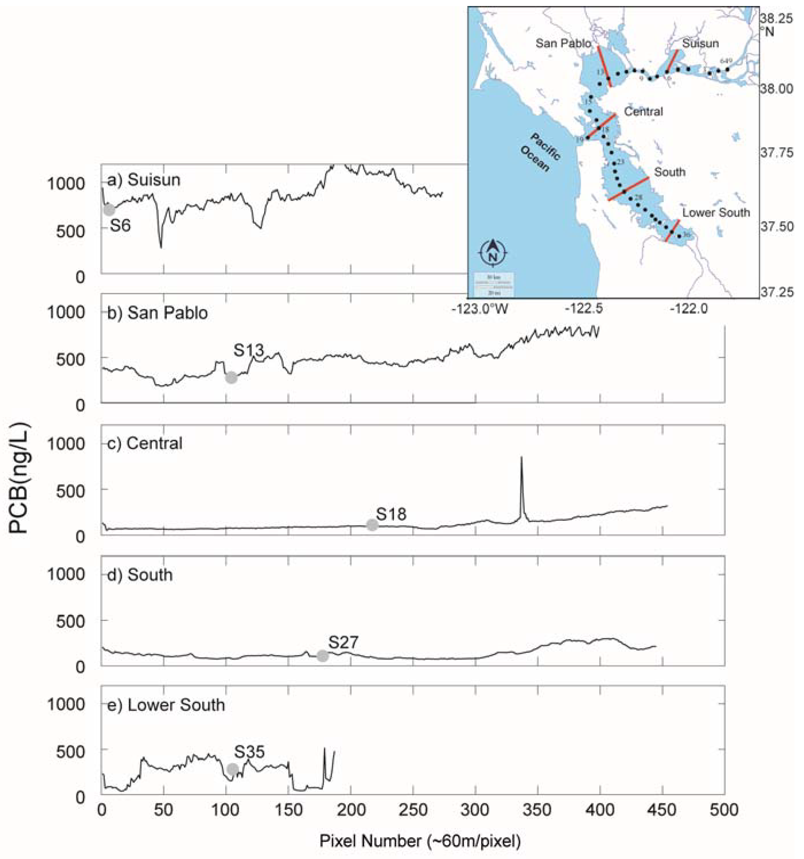
Figure 5.
To illustrate the cross-shelf variability that is not captured by traditional sampling, PCB concentration was estimated from 26 May 2016 OLI image using the entire-bay model with zero intercept (Table 1). Panels (a–e) indicate estimated cross-shelf PCB variability (solid black lines) along cross-shelf transects located in (a) Suisun, (b) San Pablo, (c) Central, (d) South, and (e) Lower South Bay. Grey circles indicate PCB concentrations estimated from UCBS-measured SSC, which spatially correspond with transects. Transect locations are indicated as red lines on the inset map (upper right-hand corner).

Figure 6.
Box plot comparing standardized PCB residuals over time across the entire SFB. Orange lines represent median values, while lower and upper box boundaries represent the 1st and 3rd quartiles (Q1 and Q3). The upper whisker represents the highest datum less than Q3 + interquartile range (IQR) × 1.5; likewise, the lower whisker represents the lowest datum greater than Q1 − 1.5 × IQR. Note the split y-axis. Open circles outlying data points.

Figure 7.
Box plot comparing residuals of in situ SPM (from USGS cruises) to SPM derived from MODIS AQUA using [20] with matchups as described in the Methods. Data were log10-transformed prior to calculating residuals. Orange lines represent median values, while lower and upper box boundaries represent the 1st and 3rd quartiles (Q1 and Q3). The upper whisker represents the highest datum less than Q3 + interquartile range (IQR) × 1.5; likewise, the lower whisker represents the lowest datum greater than Q1 − 1.5 × IQR. Open circles represent the outlying data points.


Table 1.
Statistical relationships between SFEI-sampled PCBs and SSC. a
| Area of Bay | R2 | p-Value | Empirical Relationship | RMSE (pg/L) | Mean Percent Error |
|---|---|---|---|---|---|
| Entire SFB (n = 164) | 0.33 | <0.01 | PCBs = 7.22(SSC) + 346 | 2.67 | 14.62% |
| Entire SFB b (n = 164) | 0.28 | <0.01 | PCBs = 8.84(SSC) | 3.38 | 18.12% |
| Northern Bay (n = 90) | 0.64 | <0.01 | PCBs = 3.47(SSC) + 150 | 1.91 | 10.70% |
| South-Central Bay (n = 21) | 0.80 | <0.01 | PCBs = 20.89(SSC) + 153 | 1.45 | 6.07% |
| Southern Bay (n = 53) | 0.52 | <0.01 | PCBs = 11.05(SSC) + 878 | 2.31 | 11.23% |
a Empirical relationships reported were used to remotely estimate PCBs. The entire the SFBa,b data collected February, April, July, August, 1998–2006; Northern Bay data collected February, April, July, August, 1998–2006; South-Central Bay data collected July, August, 2002–2006; Southern Bay data collected February, April, July, August, 1998–2001. All data were collected at stations within the SFB (see Figure 1 for locations). Linear regressions tested with ANCOVA are significantly different (p < 0.001). The RMSE was calculated for each relationship and is reported in PCB units (pg/L) and as a percentage of the mean. SSC represents the spatial map generated by the SSC-reflectance relationship (Table 2), which is overlain by the PCB-SSC relationship. b SSC to PCB relationship for the entire bay, with the y-intercept forced through zero.
Table 2.
Statistical relationships between satellite reflectance and USGS-sampled SSC. a
| Satellite/Atmospheric Correction | Relationship | R2 | p-Value | Empirical Relationship | log(RMSE) (mg/L) | Mean Percent Error |
|---|---|---|---|---|---|---|
| L8 OLI/Marine Correction | Rrc vs. SSC (n = 16) | 0.73 | <0.01 | SSC = 10^[13.718(Rrc) + 0.3811] | 0.62 | 48% |
| L8 OLI/Marine Correction | Rrs vs. SSC (calculated) (n = 16) | 0.77 | <0.01 | SSC = 10^[37.363(Rrs) + 0.6521] | 0.62 | 47% |
| L8 OLI/Terrestrial Correction | Rrs vs. SSC (n = 16) | 0.76 | <0.01 | SSC = 10^[0.0014(Rrs) + 0.4703] | 0.62 | 48% |
| L8 OLI/Terrestrial Correction Nechad et al. (2010) [20] | Rrs vs. TSM (n = 16) | 0.83 | <0.01 | TSM = (362.09*ρw(654))/(1 − *ρw(654)/0.1738) | 0.21 | 17.4% |
| Sentinel 2A/ACOLITE (Upper Atm Correction) | Rrc vs. SSC (n = 5) | 0.96 | <0.01 | SSC = 10^[15.98(Rrc) + 0.0493] | 0.45 | 47% |
a Red reflectance and SSC relationships. L8 OLI imagery was sampled ca. one day prior to USGS cruises (L8 OLI imagery: 06/27/2016, 07/13/2016; USGS in situ measurements: 06/28/2016, 07/14/2016). S2-MSI image was sampled the same day as USGS cruise (S2-MSI image: 07/14/2016; USGS in situ measurements: 07/14/2016). In situ data were collected in south-north transect of the SFB (see Figure 1 for locations). L8 OLI and S2-MSI images are reported with corresponding Rrs or Rrc and marine/terrestrial atmospheric correction. For the [20] algorithm, water-leaving reflectance (ρw) is used. All relationships are statistically significant at the 99% confidence level. Regressions tested with ANCOVA are highly significantly different (p < 0.001). Empirical relationships used to derive SSC from reflectance spectra are reported. RMSE for each relationship was calculated and expressed in SSC units (mg/L) and as a percentage of the mean.
© 2018 by the authors. Licensee MDPI, Basel, Switzerland. This article is an open access article distributed under the terms and conditions of the Creative Commons Attribution (CC BY) license (http://creativecommons.org/licenses/by/4.0/).
Share and Cite
MDPI and ACS Style
Hilton, A.E.; Bausell, J.T.; Kudela, R.M. Quantification of Polychlorinated Biphenyl (PCB) Concentration in San Francisco Bay Using Satellite Imagery. Remote Sens. 2018, 10, 1110. https://doi.org/10.3390/rs10071110
AMA Style
Hilton AE, Bausell JT, Kudela RM. Quantification of Polychlorinated Biphenyl (PCB) Concentration in San Francisco Bay Using Satellite Imagery. Remote Sensing. 2018; 10(7):1110. https://doi.org/10.3390/rs10071110
Chicago/Turabian StyleHilton, Annette E., Jesse T. Bausell, and Raphael M. Kudela. 2018. "Quantification of Polychlorinated Biphenyl (PCB) Concentration in San Francisco Bay Using Satellite Imagery" Remote Sensing 10, no. 7: 1110. https://doi.org/10.3390/rs10071110
Note that from the first issue of 2016, this journal uses article numbers instead of page numbers. See further details here.