Decision-Tree, Rule-Based, and Random Forest Classification of High-Resolution Multispectral Imagery for Wetland Mapping and Inventory

 , ,
, ,  , , and
Abstract
:
1. Introduction
2. Methods
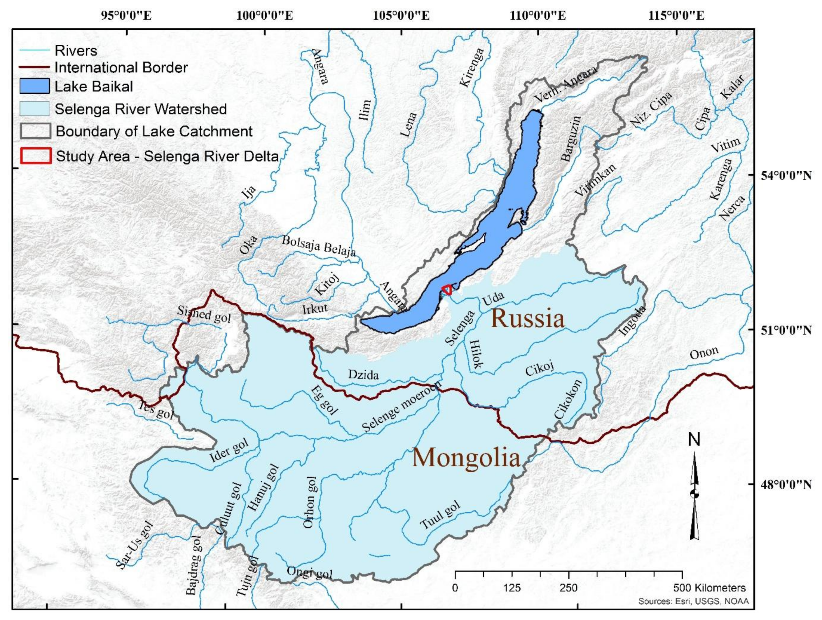
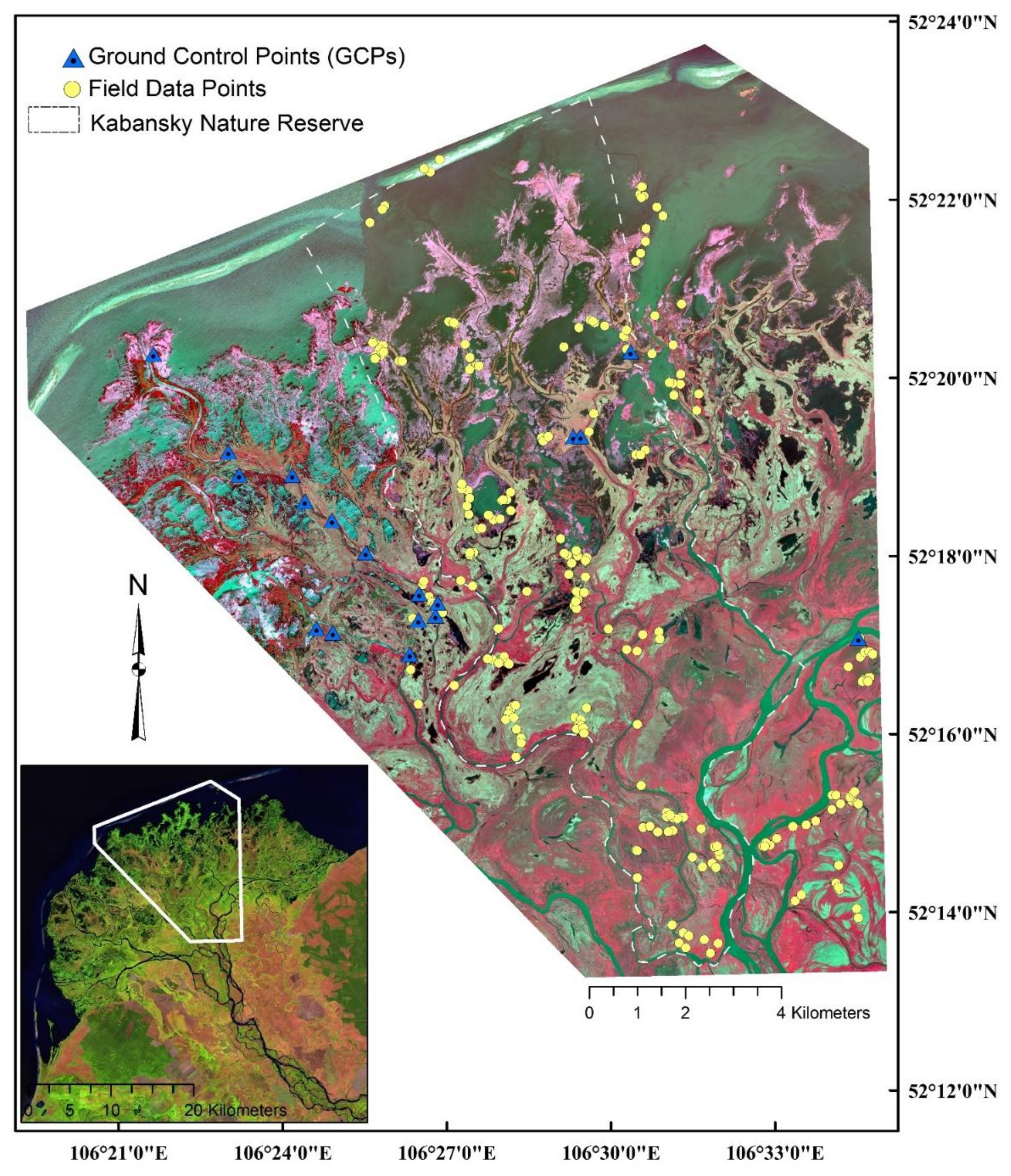
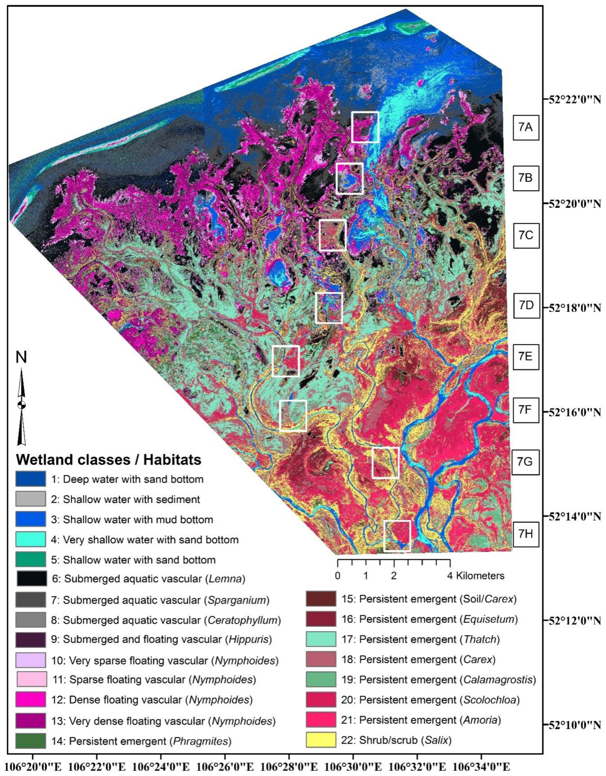
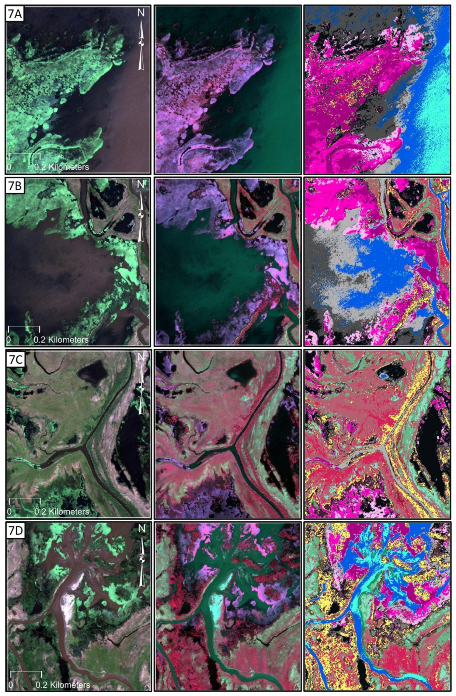
2.1. Study Area
2.2. Spatial Data, Preprocessing, and Initial Field Classifications
2.3. Field Data
2.4. Regions of Interest
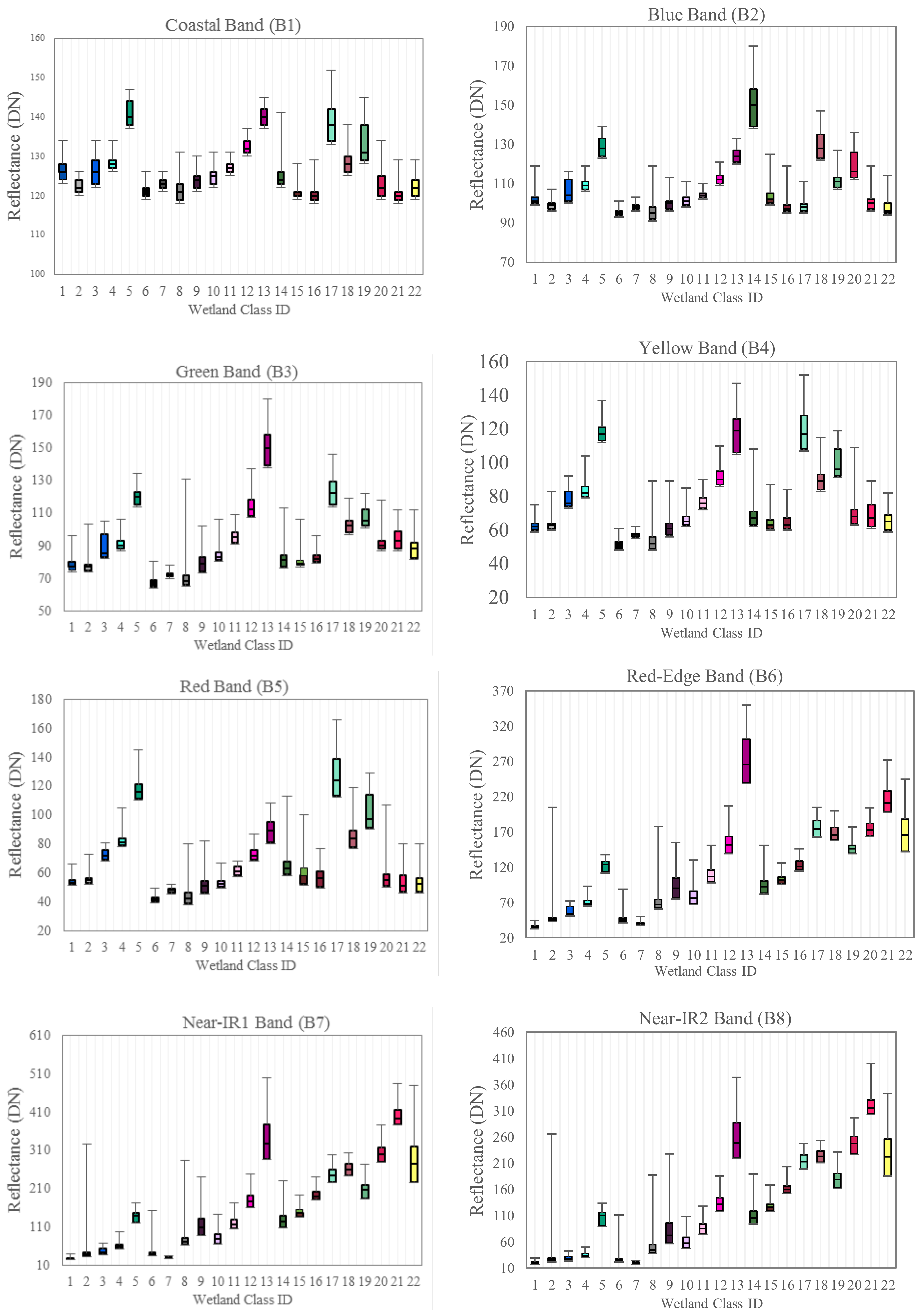
2.5. Creating Spectral Metrics
2.6. Landscape Metrics and Topographic Data
2.6.1. Landscape/Topographic Position Variable
2.6.2. Distance to Stream Channels
2.6.3. Distance to Depressional Features
2.6.4. Surface Elevation
2.7. Decision-Tree, Rule-Based, and Random Forest Classification and Assessment
2.7.1. Overview
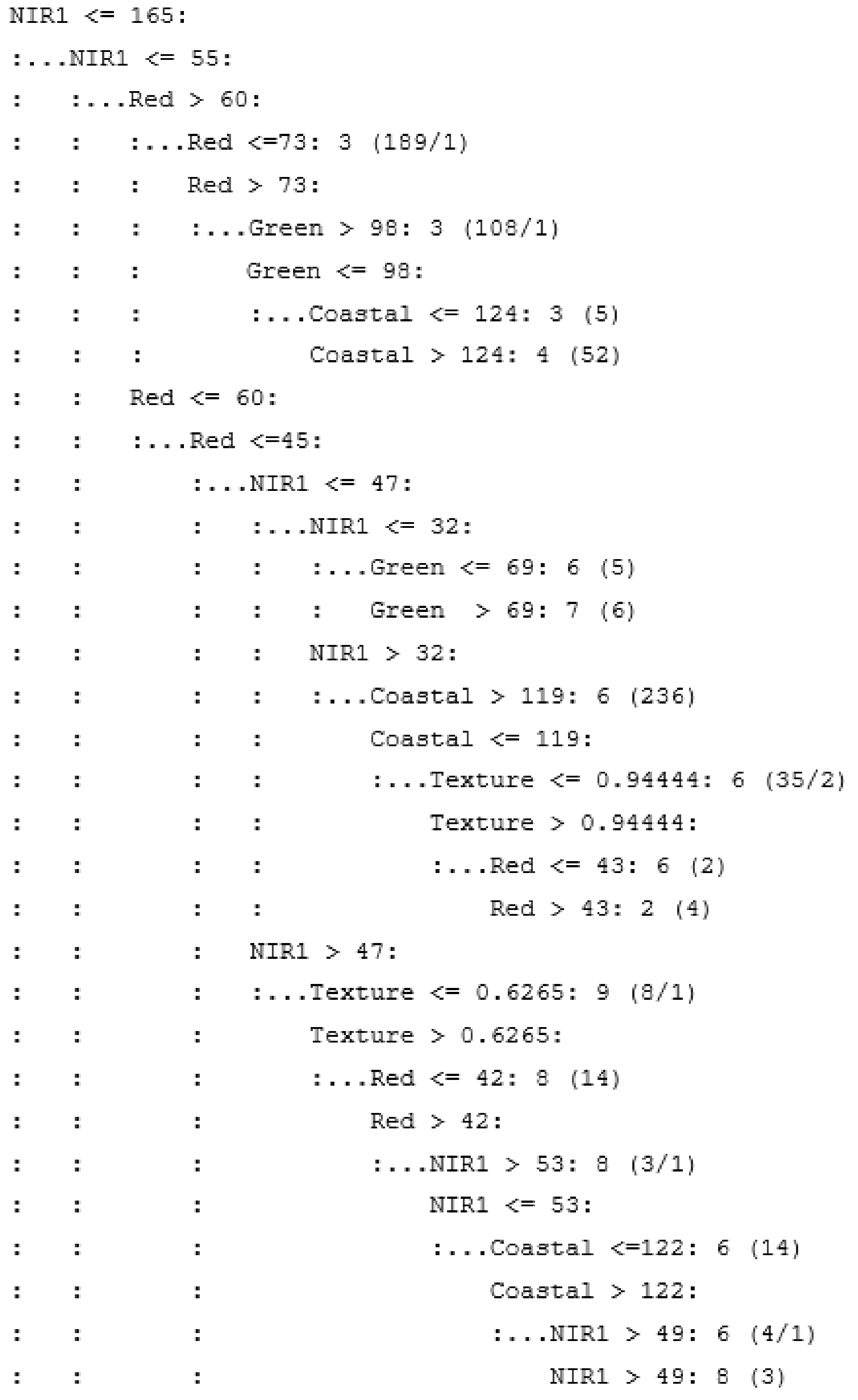
2.7.2. Decision-Tree Classification
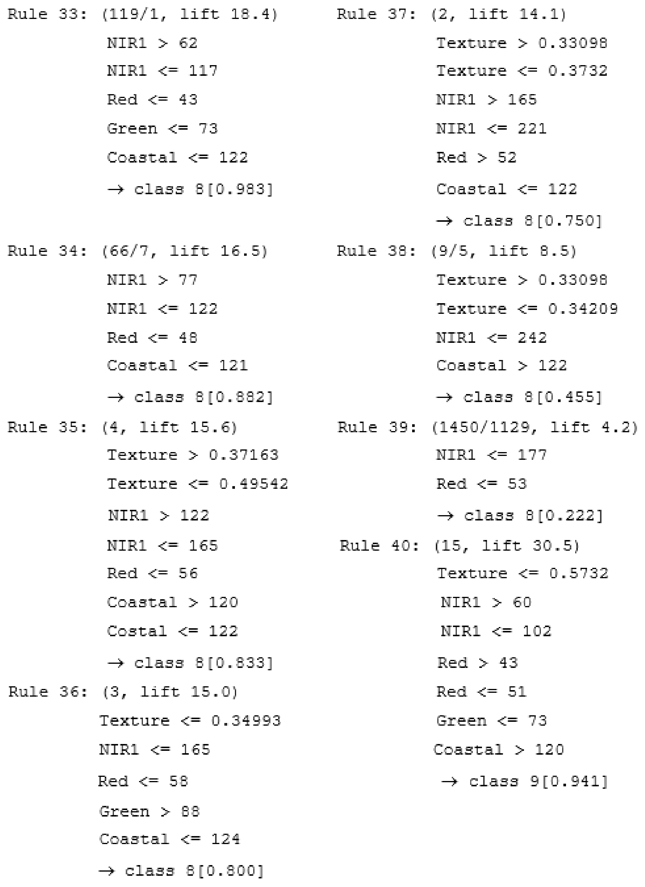
2.7.3. Rule-Based Classification
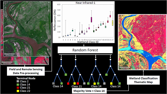
2.7.4. Random Forest Classification
2.7.5. Accuracy Assessment
3. Results
3.1. Field Data Collection
3.2. Decision-Tree, Rule-Based, and Random Forest Classification Accuracy and Complexity
3.2.1. Classification Accuracy
3.2.2. The Effects of Additional Bands and Input Parameters
4. Discussion
4.1. Random Forest as the Classifier of Choice
4.2. Overall Accuracy with a Large Suite of Classes
4.3. Metrics, Classes, Spectral Bands, and Hydrogeomorphic Variables
5. Conclusions
Acknowledgments
Author Contributions
Conflicts of Interest
References
- Titus, J.; Hudgens, D.; Trescott, D.; Craghan, M.; Nuckols, W.; Hershner, C.; Kassakian, J.; Linn, C.; Merritt, P.; McCue, T. State and local governments plan for development of most land vulnerable to rising sea level along the US Atlantic coast. Environ. Res. Lett. 2009, 4, 044008. [Google Scholar] [CrossRef]
- Klemas, V. Remote sensing of wetlands: Case studies comparing practical techniques. J. Coast. Res. 2011, 27, 418–427. [Google Scholar] [CrossRef]
- Biggs, J.; von Fumetti, S.; Kelly-Quinn, M. The importance of small waterbodies for biodiversity and ecosystem services: Implications for policy makers. Hydrobiologia 2017, 793, 3–39. [Google Scholar] [CrossRef]
- Mitsch, W.; Gosselink, J. Wetlands, 2nd ed.; Van Nostrand Reinhold Press: New York, NY, USA, 1993. [Google Scholar]
- Finlayson, C.; Davidson, N.; Spiers, A.; Stevenson, N. Global wetland inventory–current status and future priorities. Mar. Freshw. Res. 1999, 50, 717–727. [Google Scholar] [CrossRef]
- Dahl, T.E. Status and Trends of Wetlands in Conterminous United States 1986 to 1997; U.S. Fish and Wildlife Service, Branch of Habitat Assessment: Onalaska, WI, USA, 2000.
- Dahl, T.E.; Watmough, M.D. Current approaches to wetland status and trends monitoring in prairie Canada and the continental United States of America. Can. J. Remote Sens. 2007, 33, 17–27. [Google Scholar] [CrossRef]
- Creed, I.; Lane, C.; Serran, J.; Alexander, L.; Basu, N.; Calhoun, A.; Christensen, J.; Cohen, M.; Craft, C.; D’Amico, E.; et al. Enhancing protection for vulnerable waters. Nat. Geosci. 2017, 10, 809–815. [Google Scholar] [CrossRef]
- Ozesmi, S.L.; Bauer, M.E. Satellite remote sensing of wetlands. Wetl. Ecol. Manag. 2002, 10, 381–402. [Google Scholar] [CrossRef]
- Adam, E.; Mutanga, O.; Rugege, D. Multispectral and hyperspectral remote sensing for identification and mapping of wetland vegetation: A review. Wetl. Ecol. Manag. 2010, 18, 281–296. [Google Scholar] [CrossRef]
- Hess, L.L.; Melack, J.M.; Filoso, S.; Wang, Y. Delineation of inundated area and vegetation along the Amazon floodplain with the SIR-C synthetic aperture radar. IEEE Trans. Geosci. Remote Sens. 1995, 33, 896–904. [Google Scholar] [CrossRef]
- Wickham, J.; Stehman, S.; Smith, J.; Yang, L. Thematic accuracy of the 1992 National Land-Cover Data for the western United States. Remote Sens. Environ. 2004, 91, 452–468. [Google Scholar] [CrossRef]
- Wright, C.; Gallant, A. Improved wetland remote sensing in Yellowstone National Park using classification trees to combine TM imagery and ancillary environmental data. Remote Sens. Environ. 2007, 107, 582–605. [Google Scholar] [CrossRef]
- Bourgeau-Chavez, L.L.; Riordan, K.; Powell, R.B.; Miller, N.; Nowels, M. Improving wetland characterization with multi-sensor, multi-temporal SAR and optical/infrared data fusion. In Advances in Geosciences and Remote Sensing; InTechOpen Press: London, UK, 2009; pp. 679–708. [Google Scholar]
- Finlayson, C.; Valk, A.G. Wetland classification and inventory: A summary. Plant Ecol. 1995, 118, 185–192. [Google Scholar] [CrossRef]
- Guo, M.; Li, J.; Sheng, C.; Xu, J.; Wu, L. A review of wetland remote sensing. Sensors 2017, 17, 777. [Google Scholar] [CrossRef] [PubMed]
- Mahdavi, S.; Salehi, B.; Granger, J.; Amani, M.; Brisco, B.; Huang, W. Remote sensing for wetland classification: A comprehensive review. GISci. Remote Sens. 2017. [Google Scholar] [CrossRef]
- Huguenin, R.L.; Karaska, M.A.; Van Blaricom, D.; Jensen, J.R. Subpixel classification of Bald Cypress and Tupelo Gum trees in Thematic Mapper imagery. Photogramm. Eng. Remote Sens. 1997, 63, 717–724. [Google Scholar]
- Oki, K.; Oguma, H.; Sugita, M. Subpixel classification of alder trees using multitemporal Landsat Thematic Mapper imagery. Photogramm. Eng. Remote Sens. 2002, 68, 77–82. [Google Scholar]
- Stankiewicz, K.; Dabrowska-Zielinska, K.; Gruszczynska, M.; Hoscilo, A. Mapping vegetation of a wetland ecosystem by fuzzy classification of optical and microwave satellite images supported by various ancillary data. Remote Sens. Agric. Ecosyst. Hydrol. 2003, 4879, 352–361. [Google Scholar]
- Shanmugam, P.; Ahn, Y.H.; Sanjeevi, S. A comparison of the classification of wetland characteristics by linear spectral mixture modelling and traditional hard classifiers on multispectral remotely sensed imagery in Southern India. Ecol. Model. 2006, 194, 379–394. [Google Scholar] [CrossRef]
- Fournier, R.A.; Grenier, M.; Lavoie, A.; Hélie, R. Towards a strategy to implement the Canadian wetland inventory using satellite remote sensing. Can. J. Remote Sens. 2007, 33, S1–S16. [Google Scholar] [CrossRef]
- Grenier, M.; Labrecque, S.; Garneau, M.; Tremblay, A. Object-based classification of a SPOT-4 image for mapping wetlands in the context of greenhouse gases emissions: The case of the Eastmain region, Quebec, Canada. Can. J. Remote Sens. 2008, 34, S398–S413. [Google Scholar] [CrossRef]
- Wang, J.; Lang, P.A. Detection of cypress canopies in the Florida Panhandle using subpixel analysis and GIS. Remote Sens. 2009, 1, 1028–1042. [Google Scholar] [CrossRef]
- Frohn, R.; Autrey, B.; Lane, C.; Reif, M. Segmentation and object-oriented classification of wetlands in a karst Florida landscape using multi-season Landsat-7 ETM+ imagery. Int. J. Remote Sens. 2011, 32, 1471–1489. [Google Scholar] [CrossRef]
- Powers, R.P.; Hay, G.J.; Chen, G. How wetland type and area differ through scale: A GEOBIA case study in Alberta’s Boreal Plains. Remote Sens. Environ. 2011, 117, 135–145. [Google Scholar] [CrossRef]
- Hird, J.; DeLancey, E.; McDermid, G.; Kariyeva, J. Google Earth Engine, open-access satellite data, and machine learning in support of large-area probabilistic wetland mapping. Remote Sens. 2017, 9, 1315. [Google Scholar] [CrossRef]
- Ball, G.H.; Hall, D.J. ISODATA, A Novel Method of Data Analysis and Pattern Classification; DTIC Document; Stanford Research Inst. Menlo Park CA: Menlo Park, CA, USA, 1965. [Google Scholar]
- Jain, A.; Dubes, R. Algorithms for Clustering Data; Prentice Hall: Englewood Cliffs, NJ, USA, 1988. [Google Scholar]
- Jensen, J.R. Introductory Digital Image Processing, 3rd ed.; Prentice Hall: Upper Saddle River, NJ, USA, 2005. [Google Scholar]
- Foody, G.M.; Campbell, N.A.; Trodd, N.M.; Wood, T.F. Derivation and applications of probabilistic measures of class membership from the maximum likelihood classification. Photogramm. Eng. Remote Sens. 1992, 58, 1335–1341. [Google Scholar]
- Lek, S.; Guegan, J. Artificial neural networks as a tool in ecological modeling, an introduction. Ecol. Model. 1999, 120, 65–73. [Google Scholar] [CrossRef]
- Dixon, B.; Candade, N. Multispectral landuse classification using neural networks and support vector machines: One or the other, or both? Int. J. Remote Sens. 2008, 29, 1185–1206. [Google Scholar] [CrossRef]
- Mountrakis, M.; Im, J.; Ogole, C. Support vector machines in remote sensing: A review. ISPRS J. Photogramm. Remote Sens. 2011, 66, 247–259. [Google Scholar] [CrossRef]
- Breiman, L. Bagging predictors. Mach. Learn. 1996, 24, 123–140. [Google Scholar] [CrossRef]
- Quinlan, J.R. Learning decision tree classifiers. ACM Comput. Surv. (CSUR) 1996, 28, 71–72. [Google Scholar] [CrossRef]
- Quinlan, J.R. Data Mining Tools see5 and c5. 0. 2004. Available online: http://www.rulequest.com/see5-info.html (accessed on 21 March 2018).
- Kuhn, M.; Johnson, K. Classification trees and rule-based models. In Applied Predictive Modeling; Springer: New York, NY, USA, 2013; pp. 369–413. [Google Scholar]
- Hansen, M.; Dubayah, R.; DeFries, R. Classification trees: An alternative to traditional land cover classifiers. Int. J. Remote Sens. 1996, 17, 1075–1081. [Google Scholar] [CrossRef]
- DeFries, R.; Hansen, M.; Townshend, J.; Sohlberg, R. Global land cover classifications at 8 km spatial resolution: The use of training data derived from Landsat imagery in decision tree classifiers. Int. J. Remote Sens. 1998, 19, 3141–3168. [Google Scholar] [CrossRef]
- Clark, L.; Pregibon, D.; Chambers, J.; Hastie, T. Tree-Based Models. In Statistical Models in S; Routledge: Abingdon, UK, 1992; pp. 377–419. [Google Scholar]
- Baker, C.; Lawrence, R.; Montagne, C.; Patten, D. Mapping wetlands and riparian areas using Landsat ETM+ imagery and decision-tree-based models. Wetlands 2006, 26, 465–474. [Google Scholar] [CrossRef]
- Friedl, M.A.; Brodley, C.E. Decision tree classification of land cover from remotely sensed data. Remote Sens. Environ. 1997, 61, 399–409. [Google Scholar] [CrossRef]
- Li, J.; Chen, W. A rule-based method for mapping Canada’s wetlands using optical, radar and DEM data. Int. J. Remote Sens. 2005, 26, 5051–5069. [Google Scholar] [CrossRef]
- Sader, S.A.; Ahl, D.; Liou, W.-S. Accuracy of Landsat-TM and GIS rule-based methods for forest wetland classification in Maine. Remote Sens. Environ. 1995, 53, 133–144. [Google Scholar] [CrossRef]
- Houhoulis, P.F.; Michener, W.K. Detecting wetland change: A rule-based approach using NWI and SPOT-XS data. Photogramm. Eng. Remote Sens. 2000, 66, 205–211. [Google Scholar]
- Berhane, T.M.; Lane, C.R.; Wu, Q.; Anenkhonov, O.A.; Chepinoga, V.V.; Autrey, B.C.; Liu, H. Comparing pixel- and object-based approaches in effectively classifying wetland-dominated landscapes. Remote Sens. 2018, 10, 46. [Google Scholar] [CrossRef]
- Kotsiantis, S. Combining bagging, boosting, rotation forest and random subspace methods. Artif. Intell. Rev. 2011, 35, 223–240. [Google Scholar] [CrossRef]
- Belgiu, M.; Drăgut, L. Random forest in remote sensing: A review of applications and future directions. ISPRS J. Photogramm. Remote Sens. 2016, 114, 24–31. [Google Scholar] [CrossRef]
- Breiman, L. Random forests. Mach. Learn. 2001, 45, 5–32. [Google Scholar]
- Liaw, A.; Wiener, M. Classification and regression by randomForest. R News 2002, 2, 18–22. [Google Scholar]
- Tian, S.; Zhang, X.; Tian, J.; Sun, Q.R. Random forest classification of wetland landcovers from multi-sensor data in the arid region of Xinjiang, China. Remote Sens. 2016, 8, 954. [Google Scholar] [CrossRef]
- Corcoran, J.; Knight, J.; Gallant, A. Influence of multi-source and multi-temporal remotely sensed and ancillary data on the accuracy of random forest classification of wetlands in Northern Minnesota. Remote Sens. 2013, 5, 3212–3238. [Google Scholar] [CrossRef]
- Van Beijma, S.; Comber, A.; Lamb, A. Random forest classification of salt marsh vegetation habitats using quad-polarimetric airborne SAR, elevation and optical RS data. Remote Sens. Environ. 2014, 149, 118–129. [Google Scholar]
- Vanderhoof, M.K.; Alexander, L.C.; Todd, M.J. Temporal and spatial patterns of wetland extent influence variability of surface water connectivity in the Prairie Pothole Region, United States. Landsc. Ecol. 2016, 31, 805–824. [Google Scholar] [CrossRef]
- DeVries, B.; Huang, C.; Lang, M.; Jones, J.; Hiang, W.; Creed, I.; Carroll, M. Automated quantification of surface water inundation in wetlands using optical satellite imagery. Remote Sens. 2017, 9, 807. [Google Scholar] [CrossRef]
- Lane, C.R.; D’Amico, E. Calculating the ecosystem service of water storage in isolated wetlands using LiDAR in North Central Florida, USA. Wetlands 2010, 30, 967–977. [Google Scholar] [CrossRef]
- Lane, C.R.; Autrey, B.C.; Jicha, T.; Lehto, L.; Elonen, C.; Seifert-Monson, L. Denitrification potential in geographically isolated wetlands of North Carolina and Florida, USA. Wetlands 2015, 35, 459–471. [Google Scholar]
- Chalov, S.; Thorslund, J.; Kasimov, N.; Aybullatov, D.; Ilyicheva, E.; Karthe, D.; Kositsky, A.; Lychagin, M.; Nittrouer, J.; Pavlov, M.; et al. The Selenga River Delta: A geochemical barrier protecting Lake Baikal water. Reg. Environ. Chang. 2017, 17, 2039–2053. [Google Scholar] [CrossRef]
- Lane, C.R.; Liu, H.; Autrey, B.C.; Anenkhonov, O.A.; Chepinoga, V.V.; Wu, Q. Improved wetland classification using eight-band high resolution satellite imagery and a hybrid approach. Remote Sens. 2014, 6, 12187–12216. [Google Scholar] [CrossRef]
- Lane, C.R.; Anenkhonov, O.; Liu, H.; Autrey, B.C.; Chepinoga, V. Classification and inventory of freshwater wetlands and aquatic habitats in the Selenga River Delta of Lake Baikal, Russia, using high-resolution satellite imagery. Wetl. Ecol. Manag. 2015, 23, 195–214. [Google Scholar] [CrossRef]
- Khazheeva, Z.; Tulokhonov, A.; Yao, R.; Hu, W. Seasonal and spatial distribution of heavy metals in the Selenga River Delta. J. Geogr. Sci. 2008, 18, 319–327. [Google Scholar] [CrossRef]
- Brunello, A.J.; Molotov, V.C.; Dugherkhuu, B.; Goldman, C.; Khamaganova, E.; Strijhova, T.; Sigman, R. Lake Baikal Management Experience and Lessons Learned Brief. 2008. Available online: http://iwlearn.net/documents/10304 (accessed on 21 March 2018).
- Garmaev, E.J.; Khristoforov, A.V. Water Resources of the Rivers of the Lake Baikal Basin: Basics of Their Use and Protection; Geo: Novosibirsk, Russia, 2010. [Google Scholar]
- Potemkina, T. Hydrological–morphological zoning of the mouth zone of the Selenga River. Water Resour. 2004, 31, 11–16. [Google Scholar] [CrossRef]
- Moore, M.; Hampton, S.; Izmest’eva, L.; Silow, E.; Peshkova, E.; Pavlov, B. Climate change and the world’s “Sacred Sea” Lake Baikal, Siberia. Bioscience 2009, 59, 405–417. [Google Scholar] [CrossRef]
- Thorslund, J.; Jarsjö, J.; Chalov, S.R.; Belozerova, E.V. Gold mining impact on riverine heavy metal transport in a sparsely monitored region: The upper Lake Baikal Basin case. J. Environ. Monit. 2012, 14, 2780–2792. [Google Scholar] [CrossRef] [PubMed]
- Richards, J.A.; Jia, X. Feature reduction. In Remote Sensing Digital Image Analysis; Springer: Berlin/Heidelberg, Germany, 1999; pp. 239–257. [Google Scholar]
- King, R. Land cover mapping principles: A return to interpretation fundamentals. Int. J. Remote Sens. 2002, 23, 3525–3545. [Google Scholar] [CrossRef]
- Daniels, A.E. Incorporating domain knowledge and spatial relationships into land cover classifications: A rule-based approach. Int. J. Remote Sens. 2006, 27, 2949–2975. [Google Scholar] [CrossRef]
- Tucker, C.J. Red and photographic infrared linear combinations for monitoring vegetation. Remote Sens. Environ. 1979, 8, 127–150. [Google Scholar] [CrossRef]
- Gao, B. NDWI-A normalized difference water index for remote sensing of vegetation liquid water from space. Remote Sens. Environ. 1996, 58, 257–266. [Google Scholar] [CrossRef]
- Wolf, A. Using Worldview 2 Vis-NIR MSI Imagery to Support Land Mapping and Feature Extraction Using Normalized Difference Index Ratios; Digital Globe: Longmont, CO, USA, 2010. [Google Scholar]
- McFeeters, S.K. Using the normalized difference water index (NDWI) within a geographic information system to detect swimming pools for mosquito abatement: A practical approach. Remote Sens. 2013, 5, 3544–3561. [Google Scholar]
- Parviainen, M.; Zimmermann, N.; Heikkinen, R.; Luoto, M. Using unclassified continuous remote sensing data to improve distribution models of red-listed plant species. Biodivers. Conserv. 2013, 22, 1731–1754. [Google Scholar] [CrossRef]
- Sakamoto, T.; Van Nguyen, N.; Kotera, A.; Ohno, H.; Ishitsuka, N.; Yokozawa, M. Detecting temporal changes in the extent of annual flooding within the Cambodia and the Vietnamese Mekong Delta from MODIS time-series imagery. Remote Sens. Environ. 2007, 3, 295–313. [Google Scholar] [CrossRef]
- Yamagata, Y.; Yasuoka, Y. Classification of wetland vegetation by texture analysis methods using ERS-1 and JERS-1 images. In Proceedings of the IEEE International Geoscience and Remote Sensing Symposium 1993 (IGARSS’93), Better Understanding of Earth Environment, Tokyo, Japan, 18–21 August 1993; pp. 1614–1616. [Google Scholar]
- Franklin, S.E.; Peddle, D.R. Classification of SPOT HRV imagery and texture features. Remote Sens. 1990, 11, 551–556. [Google Scholar] [CrossRef]
- Haralick, R.M.; Shanmugam, K.; Dinstein, I.H. Textural features for image classification. IEEE Trans. Syst. Man Cybern. 1973, 3, 610–621. [Google Scholar]
- Gyninova, B.; Gyninova, A.; Balsanova, L. Genesis and evolution of soils in the Selenga river delta. Mosc. Univ. Soil Sci. Bull. 2008, 63, 171–177. [Google Scholar] [CrossRef]
- Gyninova, A.; Korsunov, V. The soil cover of the Selenga delta area in the Baikal region. Eur. Soil Sci. 2006, 39, 243–250. [Google Scholar] [CrossRef]
- Liu, H.; Wang, L.; Sherman, D.; Gao, Y.; Wu, Q. An object-based conceptual framework and computational method for representing and analyzing coastal morphological changes. Int. J. Geogr. Inf. Sci. 2010, 24, 1015–1041. [Google Scholar] [CrossRef]
- Frick, A.; Steffenhagen, P.; Zerbe, S.; Timmermann, T.; Schulz, K. Monitoring of the vegetation composition in rewetted peatland with iterative decision tree classification of satellite imagery. Photogramm. Fernerkund. Geoinf. 2011, 2011, 109–122. [Google Scholar]
- Hansen, M.; Defries, R.; Townshend, J.; Sohlberg, R. Global land cover classification at 1 km spatial resolution using a classification tree approach. Int. J. Remote Sens. 2000, 21, 1331–1364. [Google Scholar] [CrossRef]
- DeFries, R.; Chan, J.C.-W. Multiple criteria for evaluating machine learning algorithms for land cover classification from satellite data. Remote Sens. Environ. 2000, 74, 503–515. [Google Scholar] [CrossRef]
- Simard, M.; Grandi, G.D.; Saatchi, S.; Mayaux, P. Mapping tropical coastal vegetation using JERS-1 and ERS-1 radar data with a decision tree classifier. Int. J. Remote Sens. 2002, 23, 1461–1474. [Google Scholar] [CrossRef]
- Kearns, M.; Mansour, Y.; Ng, A.Y. An information-theoretic analysis of hard and soft assignment methods for clustering. In Learning in Graphical Models; Springer: Berlin/Heidelberg, Germany, 1998; Volume 89, pp. 495–520. [Google Scholar]
- Lakkaraju, H.; Bach, S.; Leskovec, J. Interpretable decision sets: A joint framework for description and prediction. In Proceedings of the 22nd ACM SIGKDD International Conference on Knowledge Discovery and Data Mining (KDD’16), San Francisco, CA, USA, 13–17 August 2016. [Google Scholar]
- Chan, J.; Paelinckx, D. Evaluation of random forest and adaboost tree-based ensemble classification and spectral band selection for ecotope mapping using airborne hyperspectral imagery. Remote Sens. Environ. 2008, 112, 2999–3011. [Google Scholar] [CrossRef]
- Foody, G. Classification accuracy comparison: Hypothesis tests and the use of confidence intervals in evaluations of difference, equivalence and non-inferiority. Remote Sens. 2009, 113, 1658–1663. [Google Scholar] [CrossRef]
- Rodriguez-Galiano, V.; Ghimire, B.; Rogan, J.; Chica-Olmo, M.; Rigol-Sanchez, J. An assessment of the effectiveness of a random forest classifier for land-cover classification. ISPRS J. Photogramm. Remote Sens. 2012, 67, 93–104. [Google Scholar] [CrossRef]
- Prasad, A.M.; Iverswon, L.R.; Liaw, A. Newer classification and regression tree techniques: Bagging and random forests for ecological prediction. Ecosystems 2006, 9, 181–199. [Google Scholar]
- Stumpf, A.; Kerle, N. Object-oriented mapping of landslides using random forests. Remote Sens. Environ. 2011, 115, 2564–2577. [Google Scholar] [CrossRef]
- Millard, K.; Richardson, M. On the importance of training data sample selection in random forest image classification: A case study in peatland ecosystem mapping. Remote Sens. 2015, 7, 8489–8515. [Google Scholar] [CrossRef]
- Wu, Q. GIS and remote sensing applications in wetland mapping and monitoring. In Comprehensive Geographic Information Systems; Huang, B., Ed.; Elsevier: Oxford, UK, 2018; pp. 140–157. [Google Scholar]
- Dronova, J. Object-based image analysis in wetland research: A review. Remote Sens. 2015, 7, 6380–6413. [Google Scholar] [CrossRef]
- Dubeau, P.; King, D.; Unbushe, D.; Rebelo, L. Mapping the Dabus wetlands, Ethiopia, using random forest classification of Landsat, PALSAR and topographic data. Remote Sens. 2017, 9, 1056. [Google Scholar] [CrossRef]
- Wuest, B.; Zhang, Y. Region based segmentation of Quickbird multispectral imagery through bands ratios and fuzzy comparison. ISPRS J. Photogramm. Remote Sens. 2009, 64, 55–64. [Google Scholar] [CrossRef]


| Predictor | Coastal | Blue | Green (B3) | Yellow | Red | Red-Edge | NIR1 | NIR2 | NDVI | NDSI | NDWI | LP | SD | DTS | Texture |
|---|---|---|---|---|---|---|---|---|---|---|---|---|---|---|---|
| (B1) | (B2) | (B4) | (B5) | (B6) | (B7) | (B8) | |||||||||
| Blue (B2) | 0.96 | ||||||||||||||
| Green (B3) | 0.87 | 0.88 | |||||||||||||
| Yellow (B4) | 0.93 | 0.96 | 0.93 | ||||||||||||
| Red (B5) | 0.87 | 0.95 | 0.79 | 0.94 | |||||||||||
| Red Edge (B6) | 0.42 | 0.46 | 0.75 | 0.57 | 0.40 | ||||||||||
| NIR1 (B7) | 0.21 | 0.27 | 0.56 | 0.38 | 0.26 | 0.95 | |||||||||
| NIR2 (B8) | 0.21 | 0.29 | 0.55 | 0.39 | 0.29 | 0.93 | 0.99 | ||||||||
| NDVI | −0.06 | −0.02 | 0.29 | 0.09 | −0.03 | 0.79 | 0.86 | 0.86 | |||||||
| NDSI | −0.65 | −0.69 | −0.41 | −0.70 | −0.80 | 0.02 | 0.15 | 0.10 | 0.36 | ||||||
| NDWI | −0.21 | −0.28 | −0.52 | −0.39 | −0.30 | −0.89 | −0.94 | −0.96 | −0.92 | −0.07 | |||||
| LP | −0.21 | −0.09 | −0.07 | −0.05 | 0.02 | 0.20 | 0.29 | 0.31 | 0.30 | 0.05 | −0.30 | ||||
| SD | 0.24 | 0.12 | 0.11 | 0.09 | 0.00 | −0.16 | −0.25 | −0.28 | −0.37 | −0.05 | 0.34 | −0.50 | |||
| DTS | 0.24 | 0.12 | 0.10 | 0.09 | −0.01 | −0.18 | −0.28 | −0.31 | −0.39 | −0.06 | 0.36 | −0.50 | 0.99 | ||
| Texture | 0.03 | 0.04 | −0.18 | −0.02 | 0.10 | −0.48 | −0.5 | −0.48 | −0.61 | −0.31 | 0.53 | −0.05 | 0.11 | 0.14 | |
| DEM | −0.17 | −0.05 | −0.06 | −0.03 | 0.06 | 0.16 | 0.27 | 0.31 | 0.28 | 0.00 | −0.34 | 0.48 | −0.54 | −0.53 | −0.15 |
| Test | Input Layers | Decision-Tree (DT) Classification | Rule-Based (RB) Classification | Random Forest (RF) Classification | |||||||||||
|---|---|---|---|---|---|---|---|---|---|---|---|---|---|---|---|
| Training Data | OA on Testing Data | Training Data | OA on Testing Data | Training Data | OA on Testing Data | ||||||||||
| # Tree Leaves | Error (%) | Mean (%) | 95% CI | # “If- Then” Rules | Error (%) | Mean (%) | 95% CI | Out-of-Box Error (%) | Mean (%) | 95% CI | |||||
| 1 | 4 traditional bands (B2 + B3 + B5 +B7) | 222 | 6.7 | 66.9 | 65.1 | 68.7 | 136 | 7.3 | 66.5 | 64.7 | 68.3 | 9.9 | 73.1 | 71.4 | 74.7 |
| 2 | 5 traditional bands (B1 + B2 + B3 + B5 +B7) | 252 | 5.4 | 69.2 | 67.4 | 70.1 | 157 | 6.1 | 66.6 | 64.8 | 68.4 | 8.8 | 74.0 | 72.4 | 75.7 |
| 3 | 8 traditional bands (B1-B8) | 270 | 3.5 | 73.1 | 71.4 | 74.7 | 168 | 4.0 | 74.7 | 73.0 | 76.3 | 6.6 | 76.7 | 75.1 | 78.2 |
| 4 | 8 traditional bands + NDVI | 255 | 3.4 | 73.4 | 71.7 | 75.0 | 161 | 4.0 | 73.5 | 71.8 | 75.1 | 6.8 | 75.7 | 74.0 | 77.3 |
| 5 | 8 traditional bands + NDWI | 251 | 3.5 | 72.8 | 71.1 | 74.5 | 152 | 4.1 | 73.6 | 72.0 | 75.3 | 6.6 | 77.0 | 75.4 | 78.6 |
| 6 | 8 traditional bands + NDSI | 219 | 3.5 | 73.1 | 71.4 | 74.7 | 165 | 3.8 | 71.9 | 70.2 | 73.6 | 6.6 | 77.0 | 75.4 | 78.6 |
| 7 | 8 traditional bands + texture | 226 | 2.7 | 78.2 | 76.6 | 79.7 | 156 | 3.1 | 77.7 | 76.1 | 79.2 | 4.9 | 81.1 | 79.6 | 82.6 |
| 8 | 8 traditional bands + elevation dataset | 139 | 2.2 | 61.6 | 59.8 | 63.4 | 162 | 2.5 | 61.9 | 60.0 | 63.7 | 4.2 | 75.3 | 73.6 | 76.9 |
| 9 | 8 traditional bands + 4 indices (NDVI, NDWI, NDSI, texture) | 225 | 2.4 | 77.2 | 75.6 | 78.8 | 140 | 2.9 | 78.7 | 77.2 | 80.2 | 5.1 | 80.6 | 79.0 | 82.0 |
| 10 | 8 traditional bands + 4 spectral indices; with boost (10 trials) | Boost | 0.1 | 80.1 | 78.6 | 81.6 | Boost | 0.0 | 80.0 | 78.5 | 81.5 | ||||
| 11 | 8 traditional bands + 4 spectral indices + 3 hydrogeomorphology variables | 49 | 0.8 | 55.3 | 53.4 | 57.1 | 48 | 0.8 | 54.8 | 52.9 | 56.6 | 1.6 | 74.7 | 73.1 | 76.3 |
| 12 | 8 traditional bands + 4 spectral indices + 3 hydrogeomorphology variables; with boost (10 trials) | Boost | 0.0 | 60.2 | 58.3 | 62.0 | Boost | 0.0 | 58.9 | 57.1 | 60.8 | ||||
| 13 | 8 traditional bands + 4 spectral indices + 3 hydrogeomorphology variables + elevation dataset | 153 | 0.7 | 58.0 | 56.1 | 59.8 | 100 | 0.8 | 58.3 | 56.4 | 60.1 | 1.3 | 73.0 | 71.2 | 74.5 |
| 14 | 8 traditional bands + 4 spectral indices + 3 hydro attributes + elevation dataset; with boost (10 trials) | Boost | 0.0 | 63.1 | 61.3 | 64.9 | Boost | 0.0 | 59.9 | 58.0 | 61.7 | ||||
| 15 | Uncorrelated and parsimonious (B1 + B3 + B5 + B7 + texture) | 221 | 3.4 | 75.7 | 74.0 | 77.3 | 154 | 3.9 | 74.0 | 72.4 | 75.7 | 6.2 | 81.2 | 79.7 | 82.6 |
| 16 | Uncorrelated and parsimonious (B1 + B3 + B5 + B7 + texture) with boost | Boost | 0.7 | 80.7 | 79.2 | 82.1 | Boost | 0.7 | 77.8 | 76.2 | 79.3 | ||||
| Wetland Class | 1 | 2 | 3 | 4 | 5 | 6 | 7 | 8 | 9 | 10 | 11 | 12 | 13 | 14 | 15 | 16 | 17 | 18 | 19 | 20 | 21 |
|---|---|---|---|---|---|---|---|---|---|---|---|---|---|---|---|---|---|---|---|---|---|
| 2 | 1.95 | ||||||||||||||||||||
| 3 | 2.00 | 1.96 | |||||||||||||||||||
| 4 | 2.00 | 1.99 | 1.69 | ||||||||||||||||||
| 5 | 2.00 | 2.00 | 2.00 | 2.00 | |||||||||||||||||
| 6 | 2.00 | 1.86 | 2.00 | 2.00 | 2.00 | ||||||||||||||||
| 7 | 1.94 | 1.94 | 2.00 | 2.00 | 2.00 | 1.98 | |||||||||||||||
| 8 | 2.00 | 1.80 | 2.00 | 2.00 | 2.00 | 1.54 | 1.99 | ||||||||||||||
| 9 | 2.00 | 1.66 | 2.00 | 2.00 | 2.00 | 1.74 | 2.00 | 1.12 | |||||||||||||
| 10 | 1.99 | 1.83 | 2.00 | 2.00 | 2.00 | 1.86 | 1.95 | 1.91 | 1.89 | ||||||||||||
| 11 | 2.00 | 1.96 | 2.00 | 2.00 | 2.00 | 2.00 | 2.00 | 1.99 | 1.97 | 1.34 | |||||||||||
| 12 | 2.00 | 1.99 | 2.00 | 2.00 | 2.00 | 2.00 | 2.00 | 2.00 | 1.98 | 1.90 | 1.64 | ||||||||||
| 13 | 2.00 | 1.98 | 2.00 | 2.00 | 2.00 | 2.00 | 2.00 | 1.98 | 1.92 | 1.99 | 1.95 | 1.73 | |||||||||
| 14 | 2.00 | 1.88 | 2.00 | 2.00 | 2.00 | 2.00 | 2.00 | 1.87 | 1.52 | 2.00 | 2.00 | 2.00 | 1.98 | ||||||||
| 15 | 2.00 | 1.95 | 2.00 | 2.00 | 2.00 | 2.00 | 2.00 | 1.99 | 1.87 | 2.00 | 2.00 | 2.00 | 2.00 | 1.57 | |||||||
| 16 | 2.00 | 1.97 | 2.00 | 2.00 | 2.00 | 2.00 | 2.00 | 2.00 | 1.89 | 2.00 | 2.00 | 2.00 | 2.00 | 1.82 | 1.70 | ||||||
| 17 | 2.00 | 1.99 | 2.00 | 2.00 | 2.00 | 2.00 | 2.00 | 2.00 | 1.98 | 2.00 | 2.00 | 2.00 | 2.00 | 1.93 | 1.98 | 1.94 | |||||
| 18 | 2.00 | 1.98 | 2.00 | 2.00 | 2.00 | 2.00 | 2.00 | 2.00 | 1.97 | 2.00 | 2.00 | 2.00 | 2.00 | 1.98 | 2.00 | 1.94 | 1.70 | ||||
| 19 | 2.00 | 2.00 | 2.00 | 2.00 | 2.00 | 2.00 | 2.00 | 2.00 | 2.00 | 2.00 | 2.00 | 2.00 | 2.00 | 1.98 | 2.00 | 1.99 | 1.52 | 1.69 | |||
| 20 | 2.00 | 1.98 | 2.00 | 2.00 | 2.00 | 2.00 | 2.00 | 2.00 | 1.93 | 2.00 | 2.00 | 2.00 | 1.98 | 1.98 | 2.00 | 1.95 | 1.98 | 1.79 | 1.99 | ||
| 21 | 2.00 | 2.00 | 2.00 | 2.00 | 2.00 | 2.00 | 2.00 | 2.00 | 2.00 | 2.00 | 2.00 | 2.00 | 2.00 | 2.00 | 2.00 | 2.00 | 2.00 | 2.00 | 2.00 | 1.68 | |
| 22 | 2.00 | 1.96 | 2.00 | 2.00 | 2.00 | 2.00 | 2.00 | 1.94 | 1.74 | 2.00 | 2.00 | 2.00 | 1.95 | 1.88 | 1.95 | 1.84 | 1.99 | 1.95 | 2.00 | 1.05 | 1.71 |
© 2018 by the authors. Licensee MDPI, Basel, Switzerland. This article is an open access article distributed under the terms and conditions of the Creative Commons Attribution (CC BY) license (http://creativecommons.org/licenses/by/4.0/).
Share and Cite
Berhane, T.M.; Lane, C.R.; Wu, Q.; Autrey, B.C.; Anenkhonov, O.A.; Chepinoga, V.V.; Liu, H. Decision-Tree, Rule-Based, and Random Forest Classification of High-Resolution Multispectral Imagery for Wetland Mapping and Inventory. Remote Sens. 2018, 10, 580. https://doi.org/10.3390/rs10040580
Berhane TM, Lane CR, Wu Q, Autrey BC, Anenkhonov OA, Chepinoga VV, Liu H. Decision-Tree, Rule-Based, and Random Forest Classification of High-Resolution Multispectral Imagery for Wetland Mapping and Inventory. Remote Sensing. 2018; 10(4):580. https://doi.org/10.3390/rs10040580
Chicago/Turabian StyleBerhane, Tedros M., Charles R. Lane, Qiusheng Wu, Bradley C. Autrey, Oleg A. Anenkhonov, Victor V. Chepinoga, and Hongxing Liu. 2018. "Decision-Tree, Rule-Based, and Random Forest Classification of High-Resolution Multispectral Imagery for Wetland Mapping and Inventory" Remote Sensing 10, no. 4: 580. https://doi.org/10.3390/rs10040580