Tree Crown Delineation Algorithm Based on a Convolutional Neural Network

Abstract

Tropical forests concentrate the largest diversity of species on the planet and play a key role in maintaining environmental processes. Due to the importance of those forests, there is growing interest in mapping their components and getting information at an individual tree level to conduct reliable satellite-based forest inventory for biomass and species distribution qualification. Individual tree crown information could be manually gathered from high resolution satellite images; however, to achieve this task at large-scale, an algorithm to identify and delineate each tree crown individually, with high accuracy, is a prerequisite. In this study, we propose the application of a convolutional neural network—Mask R-CNN algorithm—to perform the tree crown detection and delineation. The algorithm uses very high-resolution satellite images from tropical forests. The results obtained are promising—the $Recall$, $Precision$, and $F_1$ score values obtained were were $0.81$, $0.91$, and $0.86$, respectively. In the study site, the total of tree crowns delineated was $\mathrm{59,062}$. These results suggest that this algorithm can be used to assist the planning and conduction of forest inventories. As the algorithm is based on a Deep Learning approach, it can be systematically trained and used for other regions.

1. Introduction

Forest ecosystems are important for maintaining life on our planet, as they secure food for local population, contribute to soil conservation, mitigate the effects of climate change, and provide habitats for species and regulate water flow [1]. In particular, tropical forests have a fundamental role for maintaining biodiversity. For example, the Amazon rainforest is responsible for hosting about a quarter of the world’s terrestrial species and accounts for $15\%$ of global terrestrial photosynthesis [2]. Furthermore, tropical forests play a key role in mitigating climate change; for example, the mature Amazon rainforest absorbed the carbons emissions of all Amazonian countries across two decades (1980 to 2000) [3]. To support the construction of our knowledge on tropical forest processes, it is crucial to develop methods for large-scale forest inventories at the individual tree level to gather information on tree species, crown size, tree height, and diameter in order to estimate biomass and quantify its change through time. These tree metrics are critical for supporting applied research about tropical forest conservation, as these forests are globally threatened by widespread deforestation [4].

Traditional techniques such as field inventories, especially in tropical regions, are costly and time consuming; they cover small areas (approximately 1 hectare ($ha$)) when compared against inventories produced using a combination of remote sensing and field techniques [5,6]. For example, considering the Atlantic rainforest, an important Brazilian biome, only $0.01\%$ of its total area has been inventoried so far [7]. Forest inventories are fundamental for conservation and sustainable management, and remotely sensed aerial or satellite information could be applied to produce them [6].

With the evolution of satellite imaging technologies, the remote sensing has been getting increasingly accurate information over larger areas [8], allowing this information to be applied to forestry and monitoring deforested regions [9,10,11]. The recent availability of satellite images with very high spatial resolution (1 pixel < 1 meter (m)) allows us to observe each individual tree crown (ITC), which could enable the development of algorithms for obtaining metrics (for example, crown size) from them; thus, this information could be applied to assist the production of forest inventories [12,13]. The advantage of use metrics obtained from remote sensing data to produce forest inventories is that they could cover large areas with a lower production cost when compared to the inventories produced by a field campaign [13,14,15,16].

Previous condition for performing a forest inventory with relevant information is to apply a tree crown detection and delineation (TCDD) technique [17]. TCDD techniques help with collecting information about the number of trees in the area, a tree crown’s size, and the distance between them [13,18,19]. In addition, the TCDD with high accuracy allows a better characterization of crown’s spectral signature, a factor that can be applied to develop algorithms for species recognition [13,18,19,20]. To perform TCDD using remotely sensed images from optical passive sensors, the tree crown must be visually distinguishable, implying that spatial resolution of the image must be greater than the tree’s crown size [18]. Therefore, remotely sensed aerial or satellite images with spatial resolution in a range of 0.1–1 m/pixel allows techniques to be developed to carry out the TCDD [21]. Worldview-2 (WV-2), for example, is among the satellites that have provided optical images with very high spatial resolution which have been applied in different studies, such as those regarding species identification as well as TCDD [13,20,22].

Another promising remote sense technology applied for TCDD is the light detection and ranging (LiDAR). Several studies that used LiDAR sensors have obtained promising results in TCDD [23,24]. However, the data acquisition by LiDAR sensors is expensive and its processing is complex, which limits the reproducibility of the methods [25]. When comparing the costs of obtaining the data collected by airborne campaigns and those acquired with satellites with high spatial resolution, the latter is more affordable and provides information with multi-spectral resolution [13].

TCDD algorithms perform two distinct operations: the first is crown detection, that is, determining the location that the crown occupies, and the second is delineating the tree crown, or, in other words, determining which pixels compose the crown, to establish its borders with other trees or other elements of the scene [26]. There is a great variety of algorithms for TCDD, which can be categorized in four groups: local maximum/minimum detection [27], edge detection [28], region growing [29], and template matching [30].

TCDD approaches that use maximum/minimum location and edge detection are based on the assumption that a treetop has a mountainous structure, with a bright region at the top, and a shaded region between crowns [27,28]. The use of algorithms that are based in finding brightness pixels (called local maximum algorithms) may be useful in temperate forest regions, but this category of algorithm may not be suitable for a tropical forest region due to a large variety of tree crown formats [13]. In addition, pixels with maximum brightness may not be at the top of the crowns but in a region close to the edge; this situation can occur mainly in rounded tree crowns [13].

The techniques that use region growing are based on the crown spectral characteristics. The result of the application of this category depends on the density of the forest, the tree position and the dataset resolution [29,31]. Region growing is a segmentation approach which splits an image in different areas and recognizes objects within each sub-image. This technique depends on the assumption that the color intensity is high on the top of the tree crown and decreases gradually until the border is reached, which has a shaded area [32].

The template matching approach is based on the tree crown’s shape [31]. Generally, this approach models a tree crown using an ellipsoid (template equation), and different tree crowns shapes can be modeled by varying the ellipsoid surface (changing the ellipsoid parameters equation). Then, crowns with high correlation with the template equation are considered likely to be tree crowns [31]. Artificial neural networks (ANNs) also have been applied as a template matching step in TCDD algorithms [33,34].

Recently, a novel ANN approach, called convolutional neural network (CNN), has become the state of the art for solving different computer vision problems, such as face recognition [35], object detection [36], human pose estimation [37], and tree species detection [38]. Due to its promising results in image processing, the CNNs have been used to solve different problems within remote sensing, such as land cover classification [39], scene classification [40], object extraction [41], species classification (e.g., oil palm tree detection in a region located in the south of Malaysia [42]), fine-grained mapping of vegetation species and communities in the central Chile [43], tree crown detection [44], and very high-resolution regional tree species maps [13].

The CNN (a deep learning algorithm) is a feed-forward neural network trained in a supervised way, which has gained prominence due to its application in computer vision, mainly for solving instance segmentation problems in a scene [45]. Instance segmentation aims to identify an object at the pixel level and perform its complete delineation. Within the CNN’s architectures, the Mask R-CNN stands out, which has outperformed the results obtained by other architectures designed for instance segmentation tasks [45]. Despite the promising results reached by this CNN procedure in recent studies, such as hangar detection [46], livestock farming management [47], and ship detection [48], very little was studied about its application in high spatial resolution satellite images.

One of the main problems faced during the application of CNNs (including Mask R-CNN) is the composition of a training set with enough training examples (training patterns) for neural network learning and, hence, to solve the problem in a satisfactory way [44,45]. Deep neural networks, including CNN, require a large training set due to the number of free parameters (weights and bias) belonging to the network architecture; these free parameters need to be adjusted during the learning process. There is a directly proportional relationship between the number of free parameters and the number of patterns as input for the neural network in the training phase [49,50]. Gathering patterns for the CNN training, allowing the algorithm to solve the object detection or instance segmentation problems is costly and difficult because training sets must be composed of thousands of images, all with objects of interest with the correct delineations [44]. In addition, the quality and quantity of training patterns can impact the prediction accuracy. When using a CNN for TCDD, the collecting of training samples may become more difficult because, even in high resolution images, especially over tropical forest regions, identify ITC samples are not trivial. One solution proposed for this problem is the use of an unsupervised algorithm to select the training patterns, but the inaccuracy of this algorithm during the selection of samples for training may negatively impact the CNN’s performance [44,51]. Another alternative is the use of LiDAR point cloud information to help with the manual delineation [44].

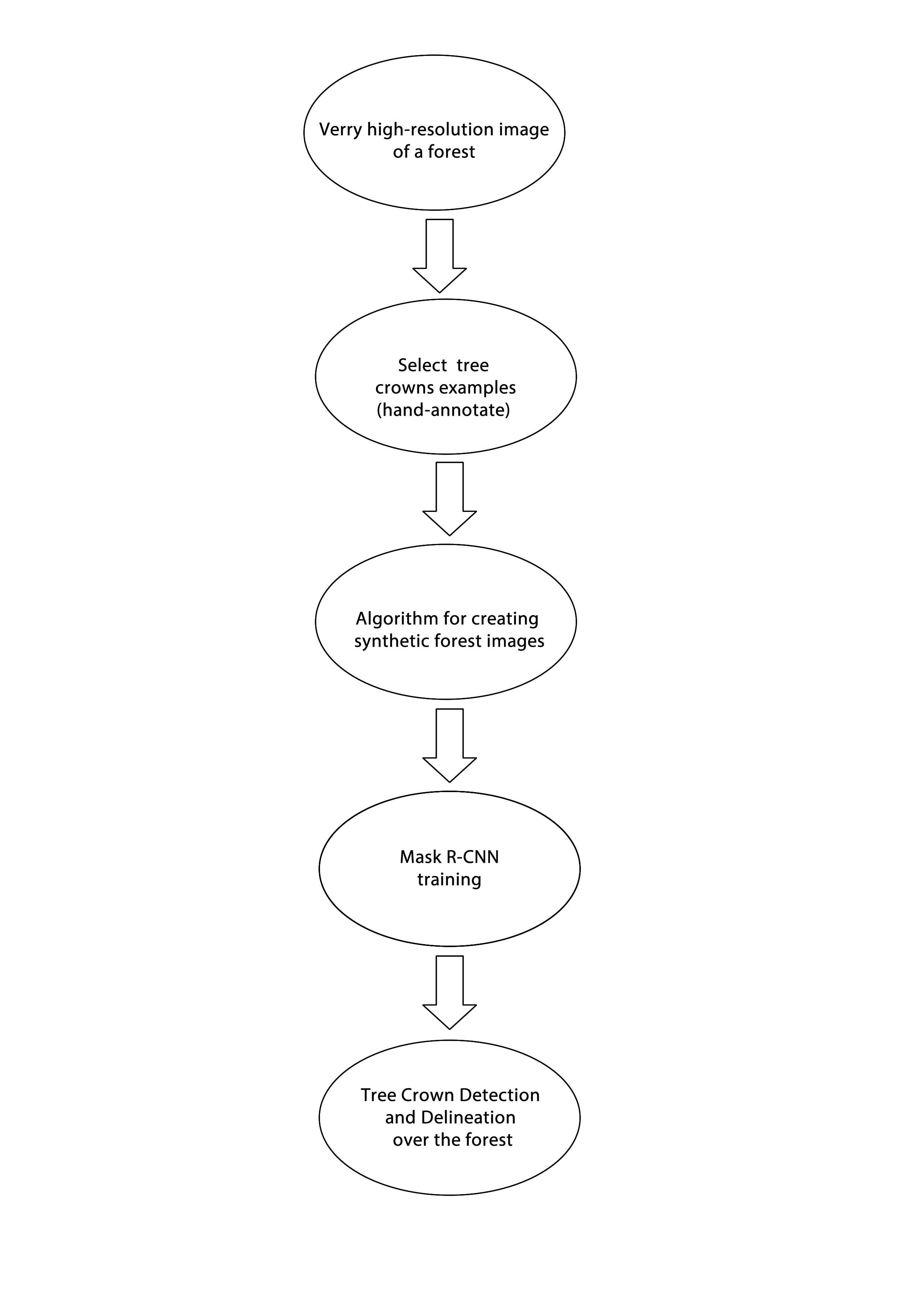
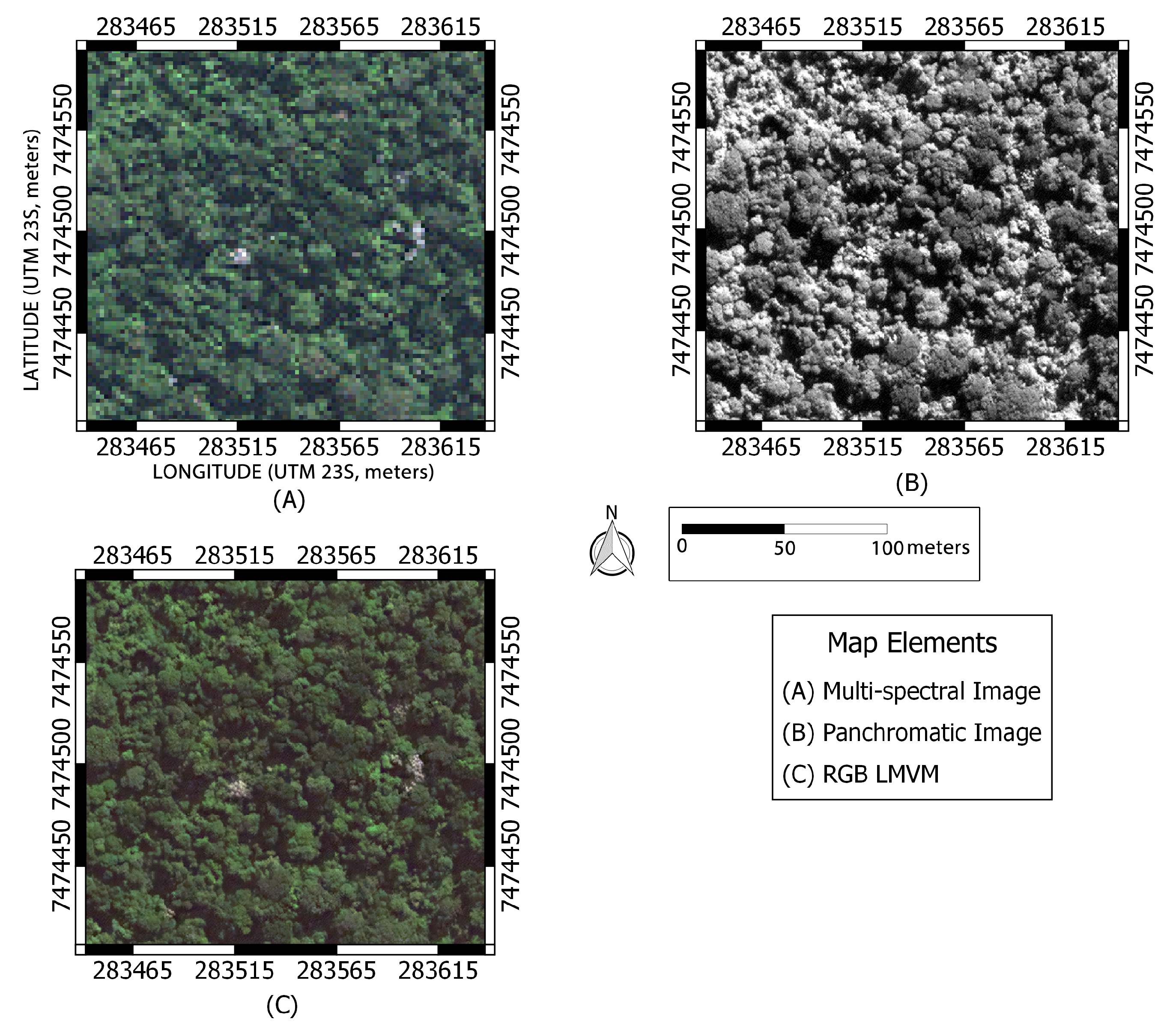
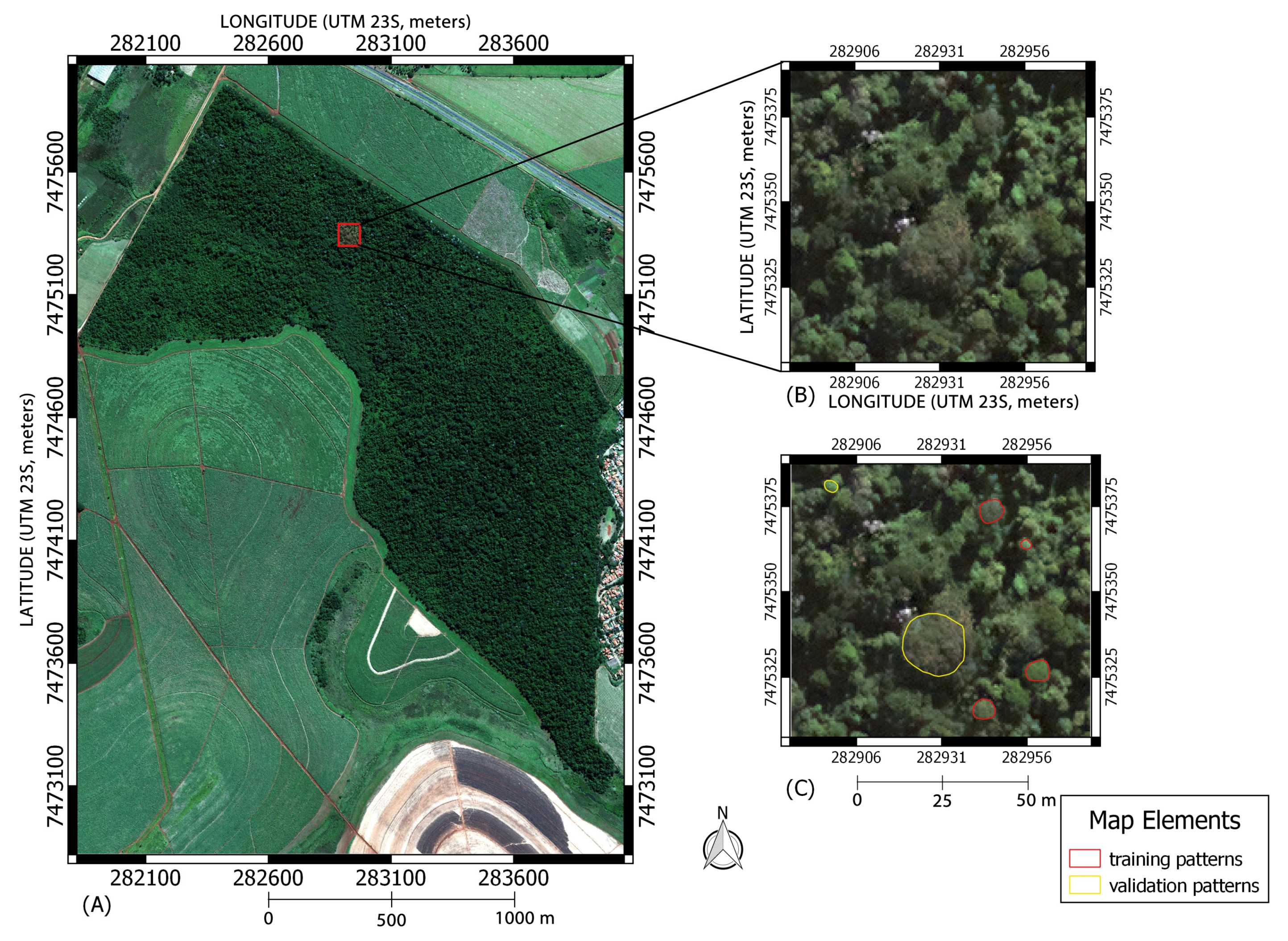
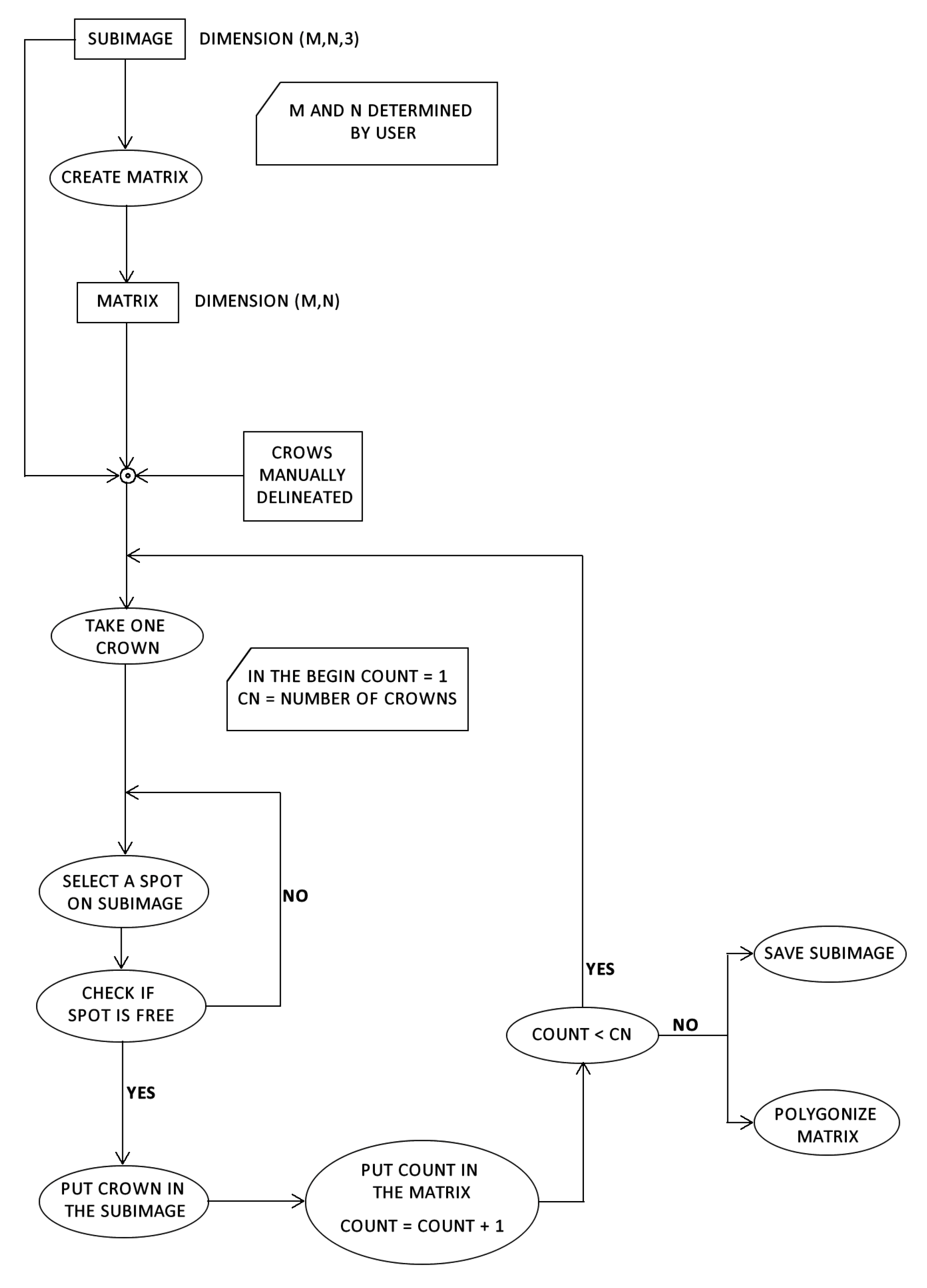
According to this context, this research proposes the application of Mask R-CNN to perform TCDD in very high spatial resolution WV-2 images ($0.5$ m per pixel) from a highly diverse tropical forest area. To construct the training set, an algorithm was implemented to obtain synthetic images. This algorithm produces the synthetic image using some hand-annotated crowns, and its implementation has two main objectives: first, to overcome the need to delineate by hand a large training set composed of images with all ITCs delineated, and, second, to evaluate its use as an alternative to other techniques (such as LiDAR and unsupervised algorithms) during the training set construction. The main objective of the study is to present a new employment of deep learning to delineate each tree crown individually in tropical forests. The main innovation presented is the use of a deep learning-based algorithm to perform the TCDD over a tropical forest image, which produces as a response the tree crown delineation. In addition, according to Weinstein et al. [44], there is a difficulty to compare results about TCDD due to variation in applied measurements; therefore, this research provides set of metrics and graphical analysis that can be used like a guideline for the analysis of others research that will perform the TCDD. For these reasons, this methodology can be applied as an auxiliary tool in the development of forest inventories of tropical regions.

2. Materials and Methods

2.1. Study Site

The study site is the Santa Genebra Forest Reserve, a remaining fragment of Atlantic tropical rainforest located in the municipality of Campinas (São Paulo State, Brazil); see Figure 1.

The Santa Genebra Reserve is located at ${22}^{\circ }{49}^{\prime }{13.46}^{″}$ S and ${47}^{\circ }{06}^{\prime }{38.47}^{″}$ W. The canopy cover in this region is highly heterogeneous and comprises deciduous and evergreen by hectare; the reserve is well-preserved and occupies an area of $237.6$ ha [20]. Surveys performed in Santa Genebra Reserve found near of 100 woody species within one hectare [52,53]. The predominant climate of the region is tropical humid, with rainfall distributed throughout the year. The region receives approximately 1500 mm of precipitation per year, but with a rainy season in the summer months (December to February) with monthly rainfall exceeding 200 mm and a drier winter (June To August) with monthly precipitation below 100 mm monthly [13].

2.2. WorldView-2 Satellite Image

The WV-2 satellite was launched in 2009 by DigitalGlobe (DigitalGlobe, Inc., Westminster, CO, USA). The WV-2 images contain eight spectral bands. The multi-spectral bands encompass the electromagnetic spectral range from 400 nm to 1500 nm with $2.0$ m of spatial resolution. The panchromatic band covers the spectrum from 450 nm to 800 nm with $0.5$ m of spatial resolution; see

Table 1. Bands name and spectral characteristics (wavelength) from WV-2 sensors.

Band Name	Band Wavelength (nm)	Band Spatial Resolution (m)
Panchromatic	450 to 800	0.5
Blue (B)	450 to 510	2.0
Green (G)	510 to 580	2.0
Red (R)	630 to 690	2.0

.

A pan-sharpening process was applied to obtain an RGB image (a combination of the red, green, and blue bands) at $0.5$ m spatial resolution (i.e., the same resolution as the panchromatic band) to produce an image which allowed the manual delineation of the tree crowns. The pan-sharpening algorithm used was the local mean variance matching (LMVM), which succeeded with yielding significant results in pan-sharpening technique comparison studies [54,55]. Figure 2 shows the results of the LMVM algorithm over a sub-image of the study area.

2.3. Individual Tree Crown Dataset

From the pan-sharpened WV-2 image, individual examples of tree crowns were manually delineated. Only crowns that are clearly identified in the satellite image were outlined to compose the training and validation set (validation during the learning process). There was no specific concern with the tree species to construct the training set. For the formation of the training set, tree crowns of different sizes, shapes, and colors were collected, so that the neural network could delineate the ITCs of any species from the Santa Genebra forest. A total of 1506 tree crowns were manually delineated, and, among them, 1050 ($69.7\%$) were selected to compose the training set and 456 ($30.3\%$) were selected to compose the validation set (validation during the neural network training), Figure 3 shows some training and validation patterns examples.

Table 2. Minimum, mean, and maximum area values for tree crowns within the validation and training sets.

	Validation Set	Training Set
Minimum Area (m${}^2$)	$3.80$	$5.12$
Mean Area (m${}^2$)	$43.93$	$49.54$
Maximum Area (m${}^2$)	$363.93$	$830.85$

shows the minimum, mean, and maximum area of ITCs in the training and validation datasets.

2.4. Instance Segmentation with Mask R-CNN

According to Bai and Urtasun [56] the instance segmentation seeks to identify the semantic class of each pixel as well as associate each pixel with a physical instance of an object. The instance segmentation is a challenge within the computer vision problems because it encompasses two hard tasks from image processing: object detection, with the purpose of classifying all the objects in the scene and locating each within a bounding box, and semantic segmentation, which seeks to determine the pixels that belong to a specific object of the scene [45,56]. The instance segmentation performs the correct delineation of different objects in a scene and gives for each object a specific number for its identification (an ID value).

The Mask R-CNN (Figure 4) is an extension of CNN, an algorithm developed to perform object detection within an image [45]. Its innovation is the inclusion of a new branch in the Faster R-CNN architecture to perform the instance segmentation [57].

The Mask R-CNN can be divided into two distinct modules that work together to perform the instance segmentation. The first module is composed of the Faster R-CNN, which performs the following operations. (i) A set of convolution layers extracts a feature map from the image. (ii) In the Faster R-CNN, there is a lightweight neural network called the region proposal network (RPN). The feature map is inputted into the RPN, and it scans the feature map and finds areas where the probability of containing an object is high; these areas are called regions of interest (RoI). (iii) Each RoI obtained from RPN could have a different shape; hence, the algorithm applies an operation (performed by a polling layer) to convert all RoI to the same shape. (iv) The fully connected networks (FCNs) work as a RoI classifier, determining the class (label) of the object and refining the location and size of the bounding box to encapsulate the object.

The second module (new branch) of Mask R-CNN is composed of a set of convolution layers which performs the masking around the object. The algorithm selects the RoIs with higher overlap precision with the ground truth (the positive RoIs). Then, the convolution layers work over the positive RoIs and determine the pixels belonging to each object. Therefore, the Mask R-CNN response is a correct bounding box, which contains the interest object and its classification within the target classes as well as the object mask, including all the pixels in the scene belonging to the object. This new branch increases the computational time, but, even with this increase in time processing, the real-time instance segmentation is still an effective solution [45].

2.5. Synthetic Forest Images for Training

In images of tropical forests, the construction of a set of samples for training a CNN is a challenge mainly due to the density of trees. The manual delineation of all the crowns in a region such as the Santa Geneva Reserve, with approximately 100 tree species per hectare, is almost impossible. To overcome this difficulty, an algorithm was developed for the creation of synthetic forest images using a set of well-delineated tree crowns created by hand. The algorithm steps are described in the Algorithm 1.

Algorithm 1. Algorithm for building a a synthetic forest image to compose the training dataset.

In the Algorithm 1:

• $subimage$ is a background where the synthetic forest will be created. Literally, it can be an image patch from a region of a WV-2 image or a black-image. The dimensions are determined by the user, but the channels must be R, G, and B;
• $polygons$ is the set of manually delineated crowns. In the specific case of this research, it is a shape-file with the geometries of each manually delineated crown;
• $count$ variable to control the numbers of crowns in the $subimage$; the algorithm copies for the $subimage$ a specific number of crowns;
• $matrix$ is a two-dimensional array which is polygonized to create the correspondent forest shape-file, where for each crown there is a geometry;
• the algorithm checks if the $place$ selected to copy the crown into the $subimage$ is free. In other words, it assesses if putting the new tree crown into the $subimage$ will cover most part of an existing tree crown;
• the $matrix$ is filled in the same selected $place$ with $count$ values.
• the $matrix$ is converted in shape-file with the geometries of each tree within; and
• the algorithm return the forest ($subimage$) image and its shape-file ($matrix$).

Figure 5 exhibits the steps of the algorithm developed to obtain a synthetic image.

2.6. Training the Mask R-CNN for TCDD

Using the algorithm for synthetic forest image creation and the vector files containing the manually delineated tree crowns, 19,656 synthetic images and their respective labels (an example in Figure 6) were created. From this sample, 15,122 were used for the Mask R-CNN training, and 4534 images were used for validation. The number of tree crowns within these synthetic forest images ranged from 4 to 150. Each synthetic image was generated with a dimension of $128\times 128$ pixels, which represents an area of 4096 m${}^2$. In the WV-2 image applied in this research, the number of tree crowns within a grid of $128\times 128$ (or 4096 m${}^2$) pixel was normally less than 150. The dimensions $128\times 128$ pixels for the synthetic images was determined to avoid problems (mainly memory allocation errors) during the training procedure. The hardware used for image processing was the main constrain that led to the definition of the dimensions of the synthetic images (hardware configuration,

Table 3. Hardware configuration applied for Mask R-CNN training and activation.

Hardware Component	Hardware Specification
Operational System	Windows 10
CPU	Intel core i7 8th Gen.
GPU	Nvidia GeForce 1070 GTX, 6 GB
RAM	32 GB

). The Mask R-CNN algorithm uses the graphics processing unit (GPU) to improve training and prediction performance. During the Mask R-CNN training on the hardware used in this research, when the neural network was fed with an image with more than 150 interest objects, the hardware could not allocate enough GPU memory to work on the image, so the computer stopped the training execution. Sometimes the training was executed, but the algorithm could not detect all the tree crowns present in the image.

The values of initial learning rate and momentum are $0.001$ and $0.9$, respectively. The training of the model was run for 120 epochs. Each epoch is a full pass over the training set. To improve the training process, a learning rate decay (a reduction in the value of the learning rate) of $\frac{learningrate}{10}$ every 40 epochs was applied. Therefore, the value of the learning rate in the epoch 41 and 81 was 1 × ${10}^{-4}$ and 1 × 10${}^{-5}$, respectively. During the training phase, data augmentation was randomly applied over the training images before they were to be inputted into the neural network. The data augmentation was composed of three image transformations (1) horizontal or vertical flip, (2) rotation of ${90}^{\circ }$, ${180}^{\circ }$ or ${270}^{\circ }$, and (3) pixel brightness value change within the range of $50\%$ to $150\%$), one of these transformations was selected and applied over a training image. Other transformations in the image, such as shearing and changing hue and saturation, were also tested, but the training with data augmentation composed by flipping, rotation, and brightness change was what produced the best results.

The metrics applied to evaluate the Mask R-CNN training and validation are class loss, bounding box loss, mask loss, and total loss. Their values after 120 epochs can be seen in

Table 4. Metrics values obtained by Mask R-CNN training and validation after 120 epochs.

Metric	Training	Validation
Class loss	$0.04$	$0.08$
Bounding box loss	$0.06$	$0.14$
Mask loss	$0.08$	$0.16$
Total loss	$0.18$	$0.38$

.

• class loss—how close the model is to predicting the correct class;
• bounding box loss—the distance between the ground-true (validation) bounding box parameters (height and width) and the prediction bounding box parameters; in other words, how good the model is at locating objects within the image;
• mask loss—measures per pixel misclassification by comparing the ground-true pixels and the predicted pixels; and
• total loss—is the sum of the others’ losses;

The stopping criterion for the neural network training was the stabilization of the total loss metric. Figure 7 shows the evolution of the total loss for both training and validation during the 120 epochs.

After the training, the Mask R-CNN was applied over the WV-2 pan-sharpened image (depicted in Figure 1B) to perform the TCDD. This image was split in patches of $128\times 128$ pixel using a regular grid with an overlap of two columns and two rows of pixels between patches, and each patch was presented to the Mask R-CNN. This overlap is important because, together with the regular grid, they help to merge a tree crown that was split by two patches. This algorithm for merging two parts of a tree crown was developed in R, and it performs the following operations: 1—selects all the tree crowns that intersect the grid lines 2—then, the algorithm checks if between two tree crowns there is an intersection (a polygon, not a line or point) between them; if so, these two segments are merged. The dimension cited in this paragraph was determined also to keep the same dimension of the training images. The Mask R-CNN output is a vector file where each tree detected in the image was delimited by a polygon with an individual identification number. All the codes developed in this research were implemented R in Python and using the libraries Tensorflow [58], Keras [59] and Gdal [60]. The Mask R-CNN algorithm was obtained from the implementation present in [61]. All the implemented codes, the Mask R-CNN for TCDD, the algorithm for creation of synthetic images, and the code for merging the tree crows split by grid is available on github: https://github.com/jgarciabraga/MASK_RCNN_TCDD.

2.7. Independent Algorithm Assessment

We conducted the algorithm validation with two main objectives: (1) to provide for future research a set of metrics (these metrics were applied in different previous research and they were summarized here) which can be applied for results analysis, thus it is possible to establish a standard for results analysis about TCDD, (2) to compare with results obtained in others previous research about TCDD, and (3) to compare to an independent evaluation dataset.

The evaluation dataset was obtained using a set of 989 points randomly generated over the Santa Genebra forest. Over these points, a visual interpretation was done, and 428 points were classified as a true crown and each one was manually delineated; 561 were marked as no crowns. Within the true crowns, the average area was 15.23 m${}^2$, the area ranged from $3.18$ m${}^2$ to $567.55$ m${}^2$, and most values ranged from $5.43$ m${}^2$ to $133.85$ m${}^2$ (the 5th and 95th percentiles, respectively).

The objective of the assessment was to obtain the algorithm’s performance in the tree crown detection accuracy and in the tree crown delineation accuracy. First, the detection accuracy was verified to evaluate the Mask R-CNN’s ability to correctly detect a tree crown in the region of tropical forest. The confusion matrix was applied with this purpose. The confusion matrix is a statistical technique, in our study, made up of two rows and two columns, which reports the number of true positive (when a true crown is detected by the algorithm), false positive (occurs when a crown is detected by algorithm where there was no crown), true negative (occurs when no crown is not detected where there was no crown) and false negative (occurs when a no crown is detected where there was a crown) [13]. Besides that, for a tree crown detected by Mask R-CNN to be classified as true positive, at least $50\%$ of its pixel must be correctly classified. When less than $50\%$ of the pixels are correctly identified, the tree crown is classified as false negative. From the confusion matrix, we computed the Kappa index [62] and the overall accuracy; these metrics were obtained to check the algorithm’s ability within the detection problem.

Other metrics were applied to evaluate the algorithm from the perspective of the automatic delineation of the tree crowns. Using the true positive results, the Mask R-CNN delineation and the manually delineation (ground-truth) were compared, and the following metrics were computed. The pixel excess (number of pixels of the segmented crown outside the true crown) and the pixel deficit (number of pixels inside the true crown missing in the segmented crown) were computed [13]. The intersection over union ($IoU$) computes the bounding box area overlapped by manual delineation and Mask R-CNN delineation (intersection area) divided by the sum of bounding boxes from the manual and neural network (union area). An object is correctly delineated when its $IoU$ was ≥50%. The $Recall$ is the value of intersection area divided by the bounding box from a manually delineated crown. The $Precision$ is the intersection area divided by the bounding box area from the object delineated by the proposal algorithm. To clarify, Figure 8 shows how to obtain the $Recall$, $Precision$, and $IoU$ values for each delineated crown.

$Recall$ and $Precision$ lead to obtaining the $F_1$ score, and this formula is exhibited in Equation (1). In the $F_1$ score, $Recall$, $Precision$, and $IoU$ are traditional metrics for evaluating delineation object algorithms, and higher values mean better algorithm result:

$$F_1=2\frac{Precision.Recall}{Precision+Recall}$$

(1)

3. Results

3.1. Detection Accuracy

From the evaluation dataset of 428 tree crowns, the algorithm correctly detected (true positive) 395 ($92.3\%$), and only 33 ($7.7\%$) were not detected (false negative). Within the 561 non-crown points (for example, a shadow), 555 ($98.9\%$) (true negative) were correctly classified, and just 6 points ($1.1\%$) were classified as a tree crown (false positives). These results can be resumed in the confusion matrix (see

Table 5. Confusion matrix obtained from Mask R-CNN tree crown detection using the algorithm evaluation dataset.

		Ground Truth
		Crown	Non-crown
Segmented	Crown	395	6
	Non-crown	33	555

).

From the confusion matrix (Table 5), we calculated the Kappa Index, which was equal to $0.919$, and the overall accuracy, equal to $96\%$. Within the group of 395 tree crowns classified as a true positive, the mean of correct pixels were $84\%$, and 345 tree crowns (or $81\%$) obtained more than $70\%$ of their pixels correctly detected.

Within the correctly detected crowns, 355 were intersected by just one tree crown. The average crown area from this group was 28 m${}^2$, and the range area varied between $3.18$ m${}^2$ and $567.54$ m${}^2$. Forty were intersected by two or more crowns as an algorithm response, and the range area within this group varied between $11.83$ m${}^2$ and $405.10$ m${}^2$, with an average of $113.20$ m${}^2$.

Table 6. The number of segments intersecting each tree canopy in the evaluation set, with respective frequency (relation to the total number of detected crowns, i.e., a total of 395).

Number of Segments	Frequency
1	355 ($89.9\%$)
2	33 ($8.4\%$)
3	4 ($1.0\%$)
4	1 ($0.2\%$)
5	2 ($0.5\%$)

presents the frequency and the number of segments that intersect the crown (i.e., the line which presents 2 segments with a frequency of 33 meanings that 33 crowns from evaluation set were intersected by 2). The number of segments was the number of tree crowns that compose a single crown.

Figure 9 shows the number of crowns by the numbers of segments, as defined by the delineation algorithm.

3.2. Delineation Accuracy

The mean area of the 395 tree crowns correctly detected was 14 m${}^2$ (56 pixels). The area value ranged from $2.75$ m${}^2$ (11 pixels) to $333.5$ m${}^2$ (1334 pixels), and the majority of the values ranged from $5.5$ m${}^2$ (22 pixels) to 127 m${}^2$ (508 pixels) (5th and 95th percentiles, respectively). The relationship between the tree crown area (in pixels) from the evaluation set and the Mask R-CNN delineation obtained a coefficient of determinations ($R^2$) of $0.9312$ (see Figure 10).

The comparison between the area (in pixels) of each canopy tree from the evaluation set and each delineated canopy resulting from the Mask R-CNN delineation were used to calculate the pixel deficit (see Figure 11A) and excess (see Figure 12A). The mean pixel deficit was $16.6\%$, and the number of tree crowns with pixel deficit was 188 ($47.6\%$ from the total of 395 detected crowns). The average area of tree crowns with pixel deficit was 49 m${}^2$. Using the graphical analysis, exhibited in Figure 11A, it was possible to note that there was no association between the validation crown size and pixel deficit, $R^2$ is equal to $-0.005$. Within the tree crowns with pixel deficit, the Mask R-CNN obtained an average area accuracy (the percentage of each crown area from evaluation set correctly determined.) of $77.7\%$, and 147 ($78.2\%$ from 183 with pixel deficit) tree crowns had an area accuracy over $70\%$; see Figure 11B.

The mean pixel excess was $25.2\%$ and the number of segmented crowns within this group was 196 ($49.6\%$ from the total of 395 detected crowns). There was no association between the validation tree crown size and pixel excess (see Figure 12A). The average area of tree crowns with pixel excess was 25 m${}^2$. The black dashed line in Figure 12A correspond to an approximation between the pixel excess and the tree crown area (from the evaluation set) by a linear model with a $R^2$ equal to $0.01$. A total of 11 ($2.8\%$) tree crowns had no pixel deficit or excess. The average area accuracy within the tree crowns with pixel excess was equal to $92.1\%$, and 191 ($97.4\%$ from 196 with pixel excess) had an area accuracy over $70\%$, see Figure 12B.

The pixel excess and deficit frequency had a normal distribution with a mean of $-6.1$ pixels and a standard deviation of $65.5$ pixels (see Figure 13).

Over a subset from Santa Genebra Reserve image (Figure 14A), the Mask R-CNN was able to delineate (Figure 14B) and to identify (give a specific ID, represented as different fill colors in; see Figure 14C) most of the visually noticeable tree crowns. This region has $\mathrm{40,501.5}$ m${}^2$ (around 4 ha) and the deep learning algorithm detected and delineated 1283 tree crowns. The subset image had a large number of trees with different crown sizes. The largest tree crown delineated by the algorithm had an area of 414 m${}^2$ and the smallest has an area of 2 m${}^2$. The average area from the delineated tree crown in this region was $12.39$ m${}^2$ and most crown areas ranged from $2.5$ m${}^2$ to $29.45$ m${}^2$ (the 5th and 95th percentiles, respectively). The total number of tree crowns delineated by Mask R-CNN in the Santa Genebra Forest was $\mathrm{59,062}$ (see Figures S1 and S2 in the Supplementary Materials).

From the 395 tree crowns detected by Mask R-CNN, 349 ($88\%$) obtained an IoU value greater than $0.5$. For the evaluation set, the average for the IoU value was $0.61$. Within the group with $IoU\ge 0.5$, the average of $IoU$ was $0.73$. Figure 15 shows the graphic of distribution of $IoU$ values and the relation between the $IoU$ value and the area (in meters) of each crown from the evaluation set.

A total of 216 ($55\%$) achieved an IoU greater than $0.7$. This IoU value indicates high fidelity to the ground truth (i.e., the hand-annotated tree crowns). In cases where the IoU value was over $0.7$, the bounding box overlay between the response and the ground truth is almost perfect (see Figure 16). In the Supplementary Materials, Figure S3 is provided, where it is possible to check the training patterns, the evaluation set, and the Mask R-CNN delineation.

Considering the evaluation set applied, the Mask R-CNN obtained an average value $F_1$ score of $0.77$ for all the tree crowns detected, and for the tree crowns with $IoU$ value $\ge 0.5$ the average for $F_1$ score was $0.86$ (see

Table 7. Average values of evaluation metrics: $Recall$, $Precision$, and $F_1$ score for all tree crowns detected by Mask R-CNN and for the tree crowns with $IoU$ value $\ge 0.5$.

Metric	Average Value (All Tree Crowns Detected)	Average Value ($\mathit{I}\mathit{o}\mathit{U}\ge 0.5$)
$Recall$	$0.68$	$0.81$
$Precision$	$0.89$	$0.91$
$F_1$ score	$0.77$	$0.86$

).

4. Discussion

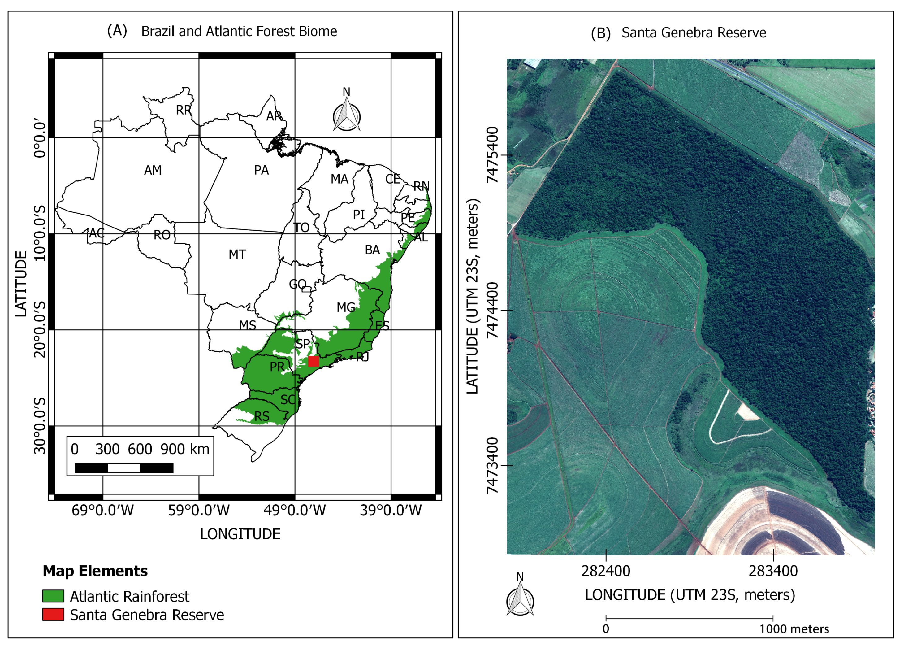
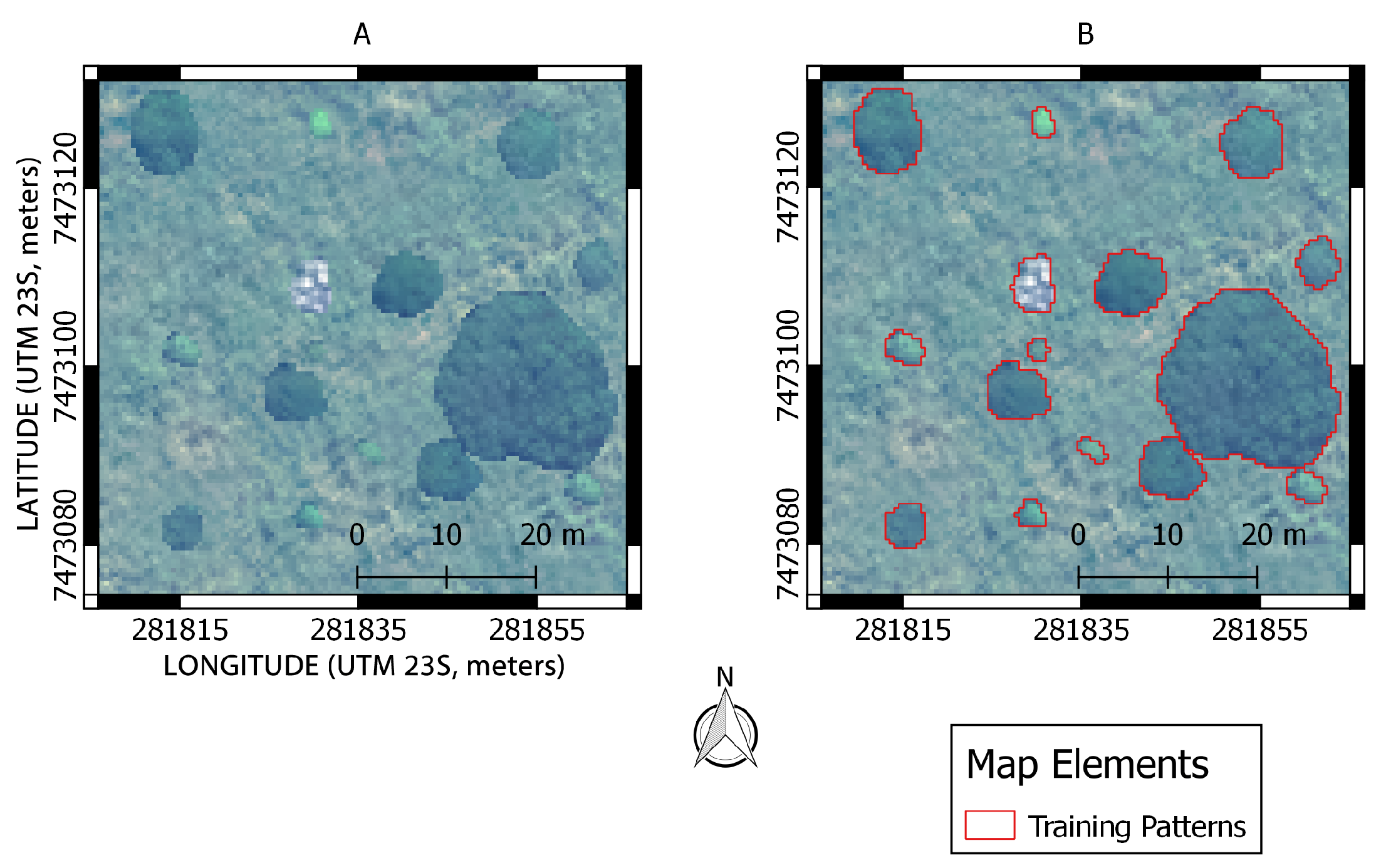
Our research proposes the application of one of the latest-developed deep learning techniques for image instance segmentation, known as Mask R-CNN [45], to perform tree crown detection and delineation in a tropical forest with a very high-resolution image. The study site was the forest of Santa Genebra Reserve, a well preserved fragment of Atlantic rainforest with a heterogeneous canopy cover [20].

One of the main difficulties faced during the work with CNN for image segmentation is building the training set, as it needs thousands of images with the object of interest manually delineated for it to be able to properly train the network. For the TCDD within a tropical forest, the difficulty to obtain images with all tree crown hand-delineated is high due to the environment complexity (e.g., the number of tree crowns and species), even using very high spatial resolution images. As an alternative to the difficulty of obtaining forest images with hand-annotated tree crown examples for deep learning training, this research uses an algorithm for the creation of synthetic forests. Using the proposed algorithm together a set of hand-delineated tree crowns, it was possible to construct thousands of synthetic forest images, as the algorithm created images with tree crown overlap and keeps the correct delineation. There is also the possibility of varying the number of tree crowns within the image, thereby allowing the creation of regions with variety in canopy density. Furthermore, each new tree crown overlay is a new pattern to be input into the neural network during the training process, which could increase its capacity in detecting tree crowns within a forest and which avoids the overfitting during the learning process.

The main advantages of the method proposed in this article include the ability to detect and delineate tree crown within a tropical forest with high accuracy and working only with an RGB satellite image to facilitate its reproduction to other areas of interest. Our findings confirmed that the CNN-based model is able to accurately detect and delineate tree crown in a highly heterogeneous tropical forest. We discuss this in greater detail in the sub-sections below the model’s performance, limitations, and perspectives.

4.1. TCDD Detection Performance

With a Kappa index and global accuracy values for tree crown detection of $0.919$ and $96\%$, respectively, Table 5), the method proposed proves to be useful for application over tropical forests. Using a number of pixels correctly detected over $70\%$, a total of 345 tree crowns were considered a true positive tree crown, and the value of Kappa index and the global accuracy were $0.813$ and $90\%$, respectively. Instead, the use of the number of pixels correctly detected to evaluate the detection accuracy, and the $IoU$ value can be used for this purpose. The research developed for [44] considered the calculus of metrics using the results with $IoU$ minimum value of $0.5$ more stringent. Our research detects 349 tree crowns with an $IoU$ value $\ge 0.5$ and 79 had an $IoU$ value $<0.5$ or were not detected. Using these values, the Kappa index obtained was $0.821$ and the global accuracy detection was $90\%$. Comparing those results obtained with a recent study on the same region, our research achieved better results, as Wagner et al. [13] obtained (for crown detection) a Kappa index value of $0.70$ and a global accuracy of $85\%$. The research developed by Wagner et al. [13] proposed an algorithm based on edge detection and region growing to perform the TCDD.

In the research developed by Larsen et al. [63], which compared six different approaches to tree crown detection algorithms, global accuracy results ranged from $32.9\%$ (region with high crown density) to $99.7\%$ (tree planting region). The six algorithms used in the research developed by Larsen et al. [63] were the region growing, treetop technique, template matching (but not a machine learning approach), scale-space, Markov random fields, and marked point process. Thus, the results obtained for detection are close to the best values obtained, with the difference that the results obtained in our research were obtained over a highly diverse tropical forest region while the results of Larsen et al. [63] were obtained over a coniferous forests.

Table 8. Comparison between the detection accuracy in the research developed by [63] (region with high crown density), Wagner et al. [13] and our research considering three situations: for tree crowns with pixels correctly detected (PCD) $\ge 50\%$; crowns with PCD $\ge 70\%$; and for tree crowns with $IoU\ge 0.5$.

Research	Algorithm	Detection Accuracy
Larsen et al. [63]	region growing	$59.2\%$
Larsen et al. [63]	treetop technique	$52.3\%$
Larsen et al. [63]	template matching	$52.6\%$
Larsen et al. [63]	scale-space	$32.9\%$
Larsen et al. [63]	Markov random fields	$47.5\%$
Larsen et al. [63]	marked point process	$49.2\%$
Wagner et al. [13]	edge detection and region growing	$85\%$
Our research (PCD ≥ $50\%$)	CNN based	$96\%$
Our research (PCD ≥ $70\%$)	CNN based	$90\%$
Our research ($IoU\ge 0.5$)	CNN based	$90\%$

summarizes the detection results obtained by Larsen et al. [63], in the region with high crown density, the detection result obtained by Wagner et al. [13], and the detection results of our research.

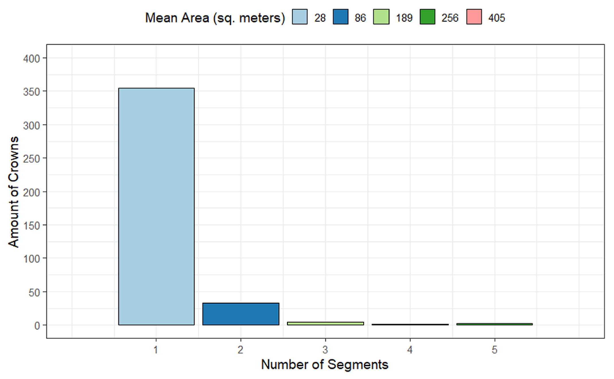
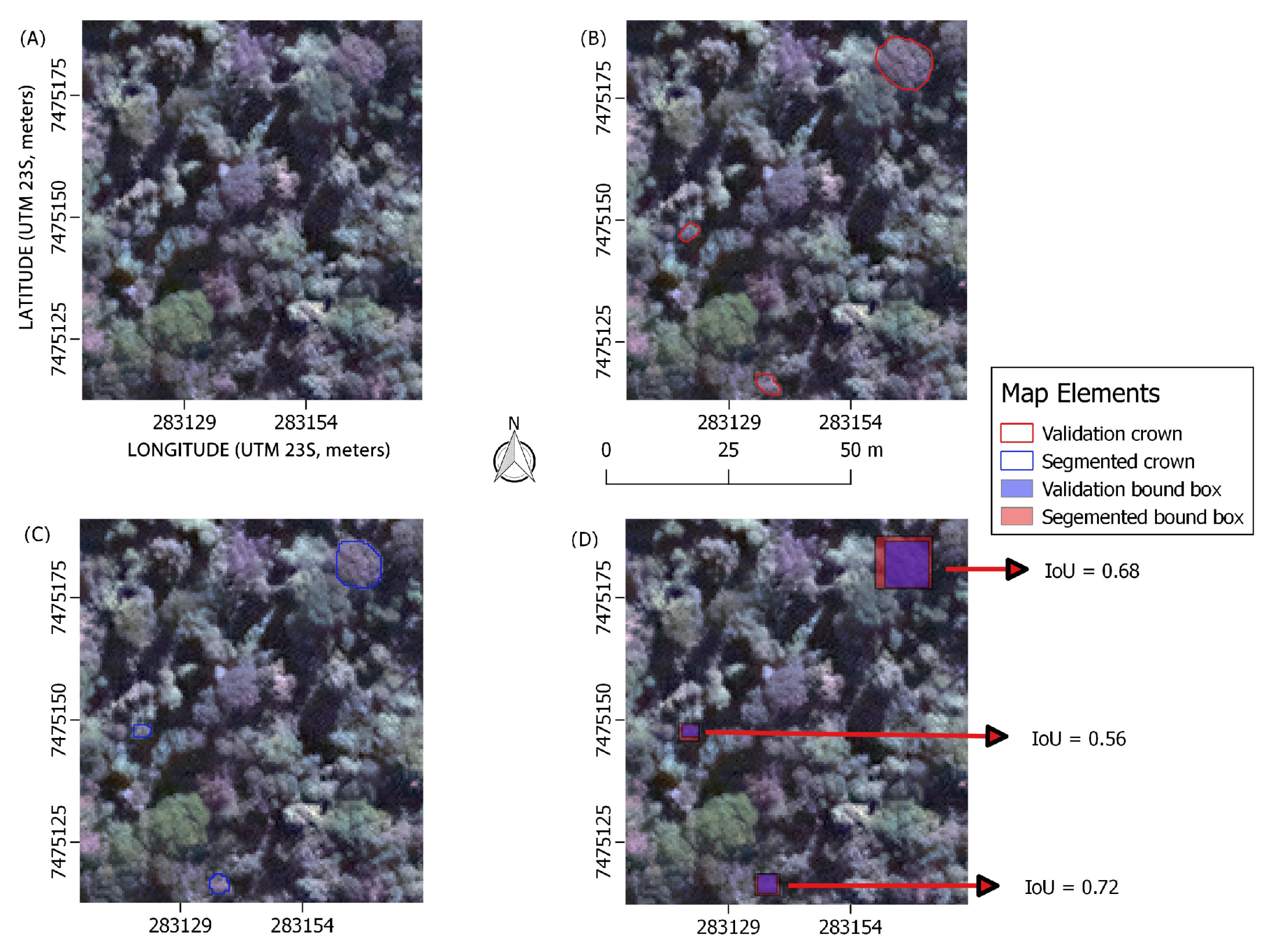
Another important result concerns the Mask R-CNN robustness in avoiding tree crown over-segmentation and under-segmentation. Over-segmentation occurs when the Mask R-CNN splits one example from the evaluation set into two or more tree crowns. Under-segmentation occurs when two or more examples from evaluation set are detected by the neural network as just one tree crown. From the total tree crowns detected by Mask R-CNN (395), $89.9\%$ were intersected by one segment. In other words, they were composed by only one tree crown (one segment); hence, they did not suffer from over-segmentation (see Table 6). Only $10.1\%$ were intersected (are composed) by two or more segments (tree crown). As shown in the graph in Figure 9, the number of segments that intersect a tree crown tends to increase with the dimensions of the crown. This occurs because the great majority of tree crowns obtained for the neural network training have a crown area smaller than 20 m${}^2$. An alternative, to circumvent this problem, could be reached introducing larger tree crowns into the training set. Under-segmentation did not occur in this research.

4.2. TCDD Delineation Performance

In this research, $88\%$ of tree crowns from the evaluation dataset obtained $IoU$ values over $0.5$ (the overall accuracy of delineation); from these tree crowns, the $Recall$, $Precision$, and $F_1$ scores values were $0.81$, $0.91$, and $0.86$, respectively. The value of $Recall$, $Precision$, and $F_1$ score considering all tree crowns detected by Mask R-CNN were respectively, $0.68$, $0.89$, and $0.77$. For semantic segmentation problems using deep learning, this result is considered significant. In the research developed by Weinstein et al. [44], a pipeline was proposed using hand-annotation examples and LiDAR data to train a CNN to perform the TCDD, the authors evaluated their research using tree different approaches for CNN’s training: the first used the hand-annotation data during the training phase, the second used a self-supervised model and the third, called a full model, combine the two previous strategies. The hand-annotated model obtained a $Recall$ of $0.38$ and a Precision value of $0.60$. The full model obtained a better result with $Recall$, $Precision$ of $0.69$, and $0.61$, respectively, with the difference that the study site used is an open woodland located in California, USA.

The study developed by Gomes et al. [64] performed the TCDD over sub-meter satellite imagery and also applied the metrics $Recall$, $Precision$, and $F_1$ for results evaluation. The algorithm proposed by [64] was based on a marked point process (MPP) to detect and delineate individual tree crowns, and the research obtained the following average values $0.67$, $0.60$, and $0.63$ for $Recall$, $Precision$, and $F_1$ score, respectively, but none of the study sites used have the same tree crown complexity of a tropical rain-forest.

Table 9. Average values of evaluation metrics $Recall$, $Precision$, and $F_1$ score of recent research that also conducted the TCDD.

Research	$\mathit{R}\mathit{e}\mathit{c}\mathit{a}\mathit{l}\mathit{l}$	$\mathit{P}\mathit{r}\mathit{e}\mathit{c}\mathit{i}\mathit{s}\mathit{i}\mathit{o}\mathit{n}$	${\mathit{F}}_1$ Score
Silva et al. [65] obtained from [44]	$0.14$	$0.07$	$0.09$
Gomes et al. [64]	$0.67$	$0.60$	$0.63$
Weinstein et al. [44] hand-annoted ($IoU\ge 0.5$)	$0.38$	$0.60$	$0.47$
Weinstein et al. [44] full model ($IoU\ge 0.5$)	$0.69$	$0.61$	$0.65$
Our (this) Research ($IoU\ge 0.5$)	$0.81$	$0.91$	$0.86$

summarizes the value of $Recall$, $Precision$, and $F_1$ score of recent research that performed TCDD over sub-meter satellite imagery.

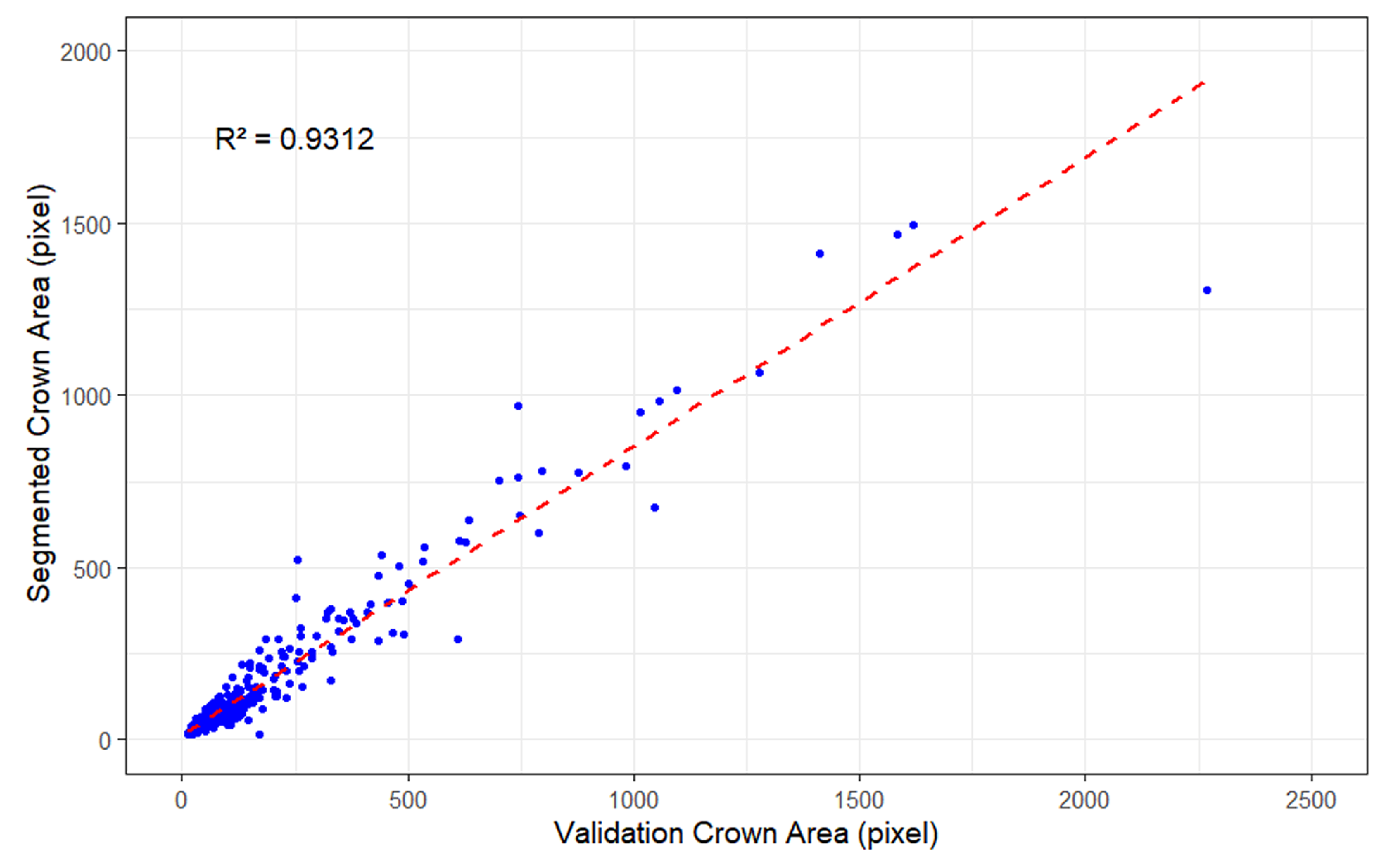
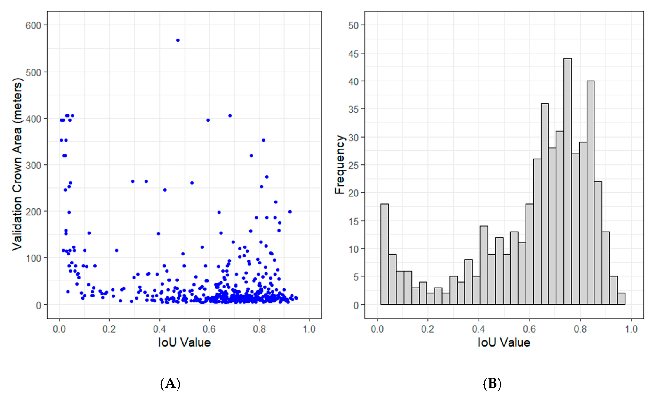
With the overall accuracy rate of $88\%$, our method proves to be useful for performing the TCDD because recent research of TCDD algorithm development has obtained close accuracy values; Tochon et al. [25], and Singh et al. [15] have reported accuracy of $68\%$ and $69.2\%$, respectively, Wagner et al. [13] has reported $80\%$ and Dalponte et al. [66] achieved $88.8\%$. Moreover, the relationship between the tree crown area (in pixels) of examples from the evaluation set and tree crown area (in pixels) obtained by the proposed segmentation algorithm, Figure 10, has a value of $R^2$ of $0.9312$, which demonstrates the robustness of the Mask R-CNN to estimate the crowns dimensions and hence to perform the tree crown delineation.

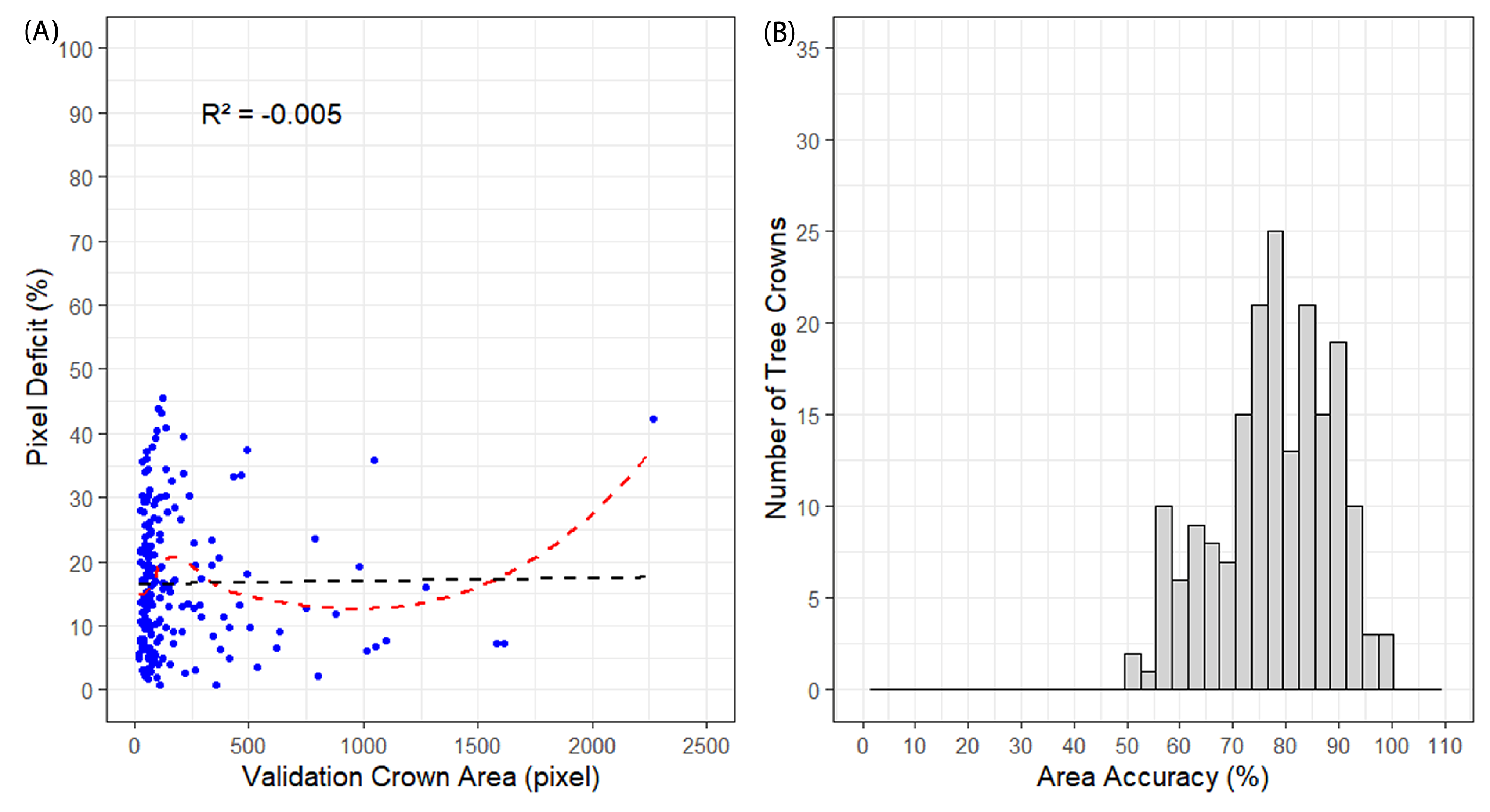
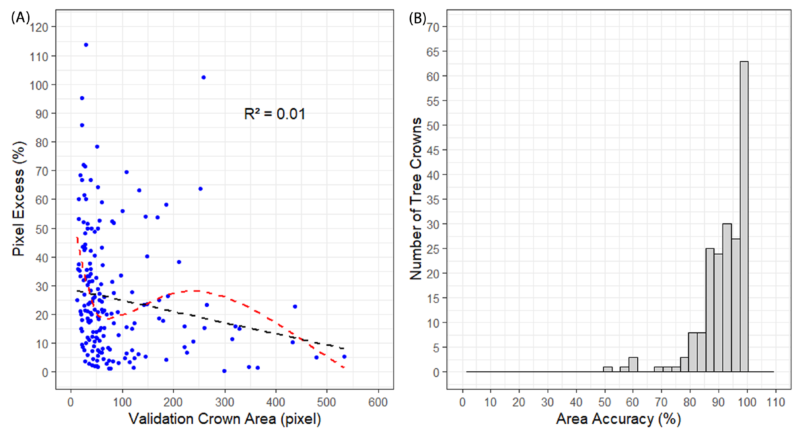
Dalponte et al. [66] reported that the size of small treetops tends to be underestimated when optical images are applied in the TCDD process. In our study, this problem did not occur since there is no relationship between pixel deficit and tree crown area (see Figure 11). Pixel deficit occurs mainly in larger tree crowns (see Figure 11). In addition, our results show that the tree crowns with the smallest area have the best value of $IoU$; see Figure 15A.

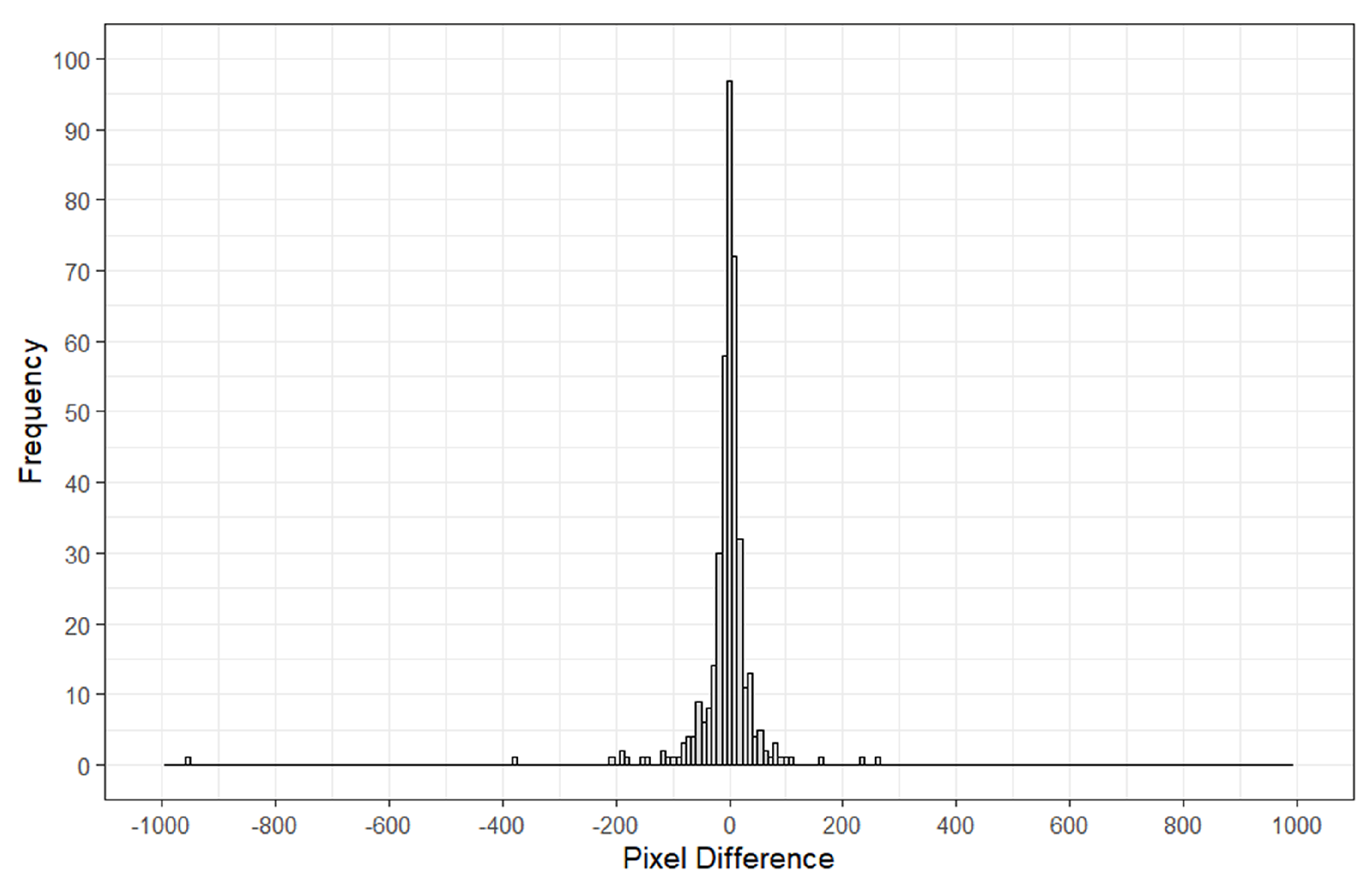
However, the proposed algorithm tended to overestimate the tree crown area because the number of examples of excess pixel crowns is greater when compared to the number of examples with pixel deficit (see Figure 11 and Figure 12). The overestimated areas occur mainly in tree crowns with area less than $12.5$ m${}^2$ (see Figure 12), but the result for the crown delineation was not significantly impaired because the pixel difference between the segmented tree crowns and the evaluation tree crowns had a normal distribution with a mean of –6 pixels (see Figure 13) and an $IoU$ value distribution greater than $0.5$ for $88\%$ of examples. In addition, the $F_1$ score achieved significant values, over $0.70$.

In this research, the total of tree crowns detected and delineated by Mask R-CNN was of $\mathrm{59,062}$, and the tree crown area ranges from 2 m${}^2$ to $413.75$ m${}^2$ (see Figure S1 in the Supplementary Materials). The average crown area was $8.75$ m${}^2$ and the most part of the area ranged from $3.75$ m${}^2$ to 34 m${}^2$ (the 5th to 95th percentiles, respectively). In the research developed by Wagner et al. [13], which implemented a traditional TCDD algorithm to work over the Santa Genebra Forest Reserve, only 23,278 tree crowns were detected and delineated.

4.3. Algorithm Requirements

4.3.1. Shade Effect—Limitations and How to Resolve Them

One of the main issues for the accuracy of TCDD algorithm is the shade effect [13,66], and, in our analysis, some tree crowns present in shadow regions were ignored by the model, Figure 14. According to Dalponte et al. [66], the shadow effect in TCDD algorithms could be solved using LiDAR data. Considering the TCDD performed by a neural network approach, to decrease the shadow effect, another strategy to work around the problem using multi-spectral images could be to feed the model with a labeled image of trees present in a shadow region during the neural network training.

4.3.2. How to Deal with the Leaf Fall Effect

The image of this study was taken during the wet season, when all crowns are likely foliated. However, the Santa Genebra reserve is a seasonal semi-deciduous forest with a leaf loss ranging from $20\%$ to $50\%$ during the dry season [20] plus seasonal changes in spectral characteristics [67]. These characteristics could increase the shadow presence and decrease the algorithm accuracy. As the algorithm presented in this research is based on a supervised neural network, to handle with leafless tree crowns, the presentation of images with leafless trees during training can be an alternative to reduce algorithm errors. Moreover, with the adoption of this alternative, the algorithm could operate over images taken throughout the year. Further works are needed to improve the training sample of the model and limit the effects of shade and seasonal changes in reflectance.

4.3.3. Algorithm Limitations

The prediction of the algorithm was made on patches of $128\times 128$ pixels in a grid approach; between the patches, there is an overlap of two columns and rows of pixels, and then the prediction for each patch were merged. After the prediction, the algorithm that performs the tree crown merging is applied to make the union between the crown which was split by the grid.

The grid size ($128\times 128$ pixels) is not a requirement of the algorithm but was designed to deal with the limitation of the GPU hardware, mainly the memory (hardware configuration Table 3). However, more recent hardware could make the prediction with a larger grid size.

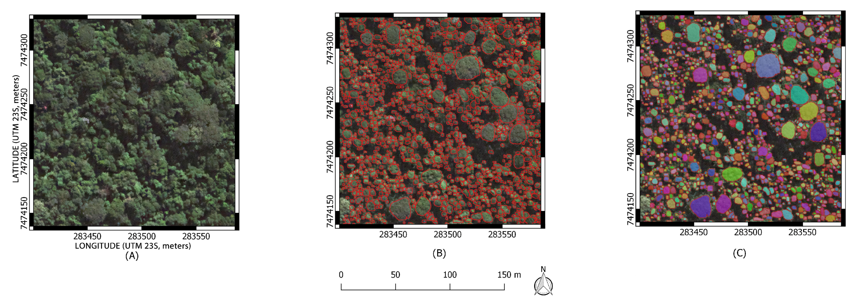
Through a visual analysis of Figure 14B, it is possible to observe that the algorithm that performs the tree crown merging works correctly. However, if a different grid size is adopted, this algorithm must be modified because it was developed to solve the merging following the limitations of this research.

4.4. Algorithm’s Advance

Since the launch of Ikonos in 1999, a great number of very high-resolution optical imagery from different satellites (e.g., WorldView, Geoeye, and Quickbird) have become available for the study of ITCs. The development of automatic techniques to perform the TCDD using imagery from these satellites have attracted attention from research from image processing, remote sensing, and forestry [26,64].

Most of the algorithms which perform the TCDD on very high-resolution satellite imagery were developed to work on specific regions of temperate forests [26]. Typically, these algorithms use techniques such as region growing, edge detection, local maximum, and template matching (with a specific geometric form, such as an ellipse) [64]. The use of these algorithms over tropical forests may be very difficult as they could need several configurations because, in these regions, the ITCs are not so homogeneous (size and shapes are different) and their spectral characteristics and texture vary widely. However, the application of our technique could be extended to any type of region (for example, temperate forests or other tropical forests) because it depends only some hand-annotated ITCs to feed the algorithm of synthetic image creation.

Tropical forests can be composed of a great amount of tree crowns with extensive variety of colors, sizes, and shapes, and even using very high-resolution images is difficult (or impossible) to hand-annotate all ITCs within a specific region. For the training of a delineation algorithm based on a CNN approach, all the ITCs within the imagery of the training set must be annotated, or else the algorithm does not converge to a desired response. Therefore, our approach, which uses the creation of synthetic images, could be an alternative to overcome the need to hand-annotate all tree crowns within a tropical forest region. Besides that, our technique proved to be useful because it achieved the $F_1$ score and the $IoU$ average value of $0.86$ and $0.73$, respectively (considering the Mask R-CNN response with $IoU\ge 0.5$).

4.5. Application Perspectives

An important aspect of tropical forests is that their biomass is concentrated in large trees [68]. The research developed by Blanchard et al. [69] shows that the relationship between diameter breast height and crown area for individual trees, within tropical regions, is stable with no significant variation. In a perspective for biomass estimation, our delineation algorithm could be applied for this purpose using optical images and large-scale assessments using optical imagery. However, a more detailed work applying our method and validation analyses over different forested areas are still needed to support this idea. For example, field data can be used to calibrate our algorithm and then use its answer to estimate the biomass and biomass change of large area using high resolution satellite images.

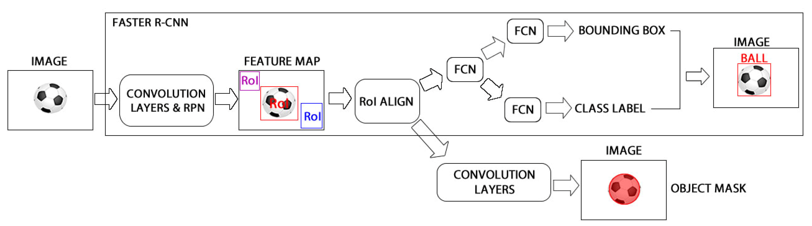
Another perspective for a possible application of our algorithm of TCDD is related to mapping species. In the research developed in the same forest site by Wagner et al. [13], Ferreira et al. [67], after the delineation, support vector machines (SVMs) were successfully applied to determine the species of each delineated tree crown, showing that spectral information could be used to predict the species. The Mask R-CNN could also be applied to mapping species. The Mask R-CNN works with two distinct modules: (i) one to determine the bounding box of the object of interest; and (ii) another to determine the pixels belonging to each object of interest (see Figure 4). These two modules are formed by a set of convolutional layers, also known as convolutional filters. In the module formed by Faster R-CNN, the convolutional filters closest to the input layers are responsible for detecting the low-level features. On the other hand, the last convolutional filters from Faster R-CNN are more specialized and they are responsible for detecting the high-level features. Thus, an analysis over the response of high level filter from Mask R-CNN (mainly those that compose the Faster R-CNN) could be applied to identify the filters that are activated during the prediction; the features set obtained from these filters can be applied to perform a more specialized image segmentation, such as species classification. A review about CNN filter analysis can be obtained in Bilal et al. [70]. For example, after the delineation, the high level feature information can be obtained from high level filters and used for specie recognition, since each tree is delineated as a unique object for our algorithm, and another machine learning technique (other CNN or even the Mask R-CNN) could be used to analyze those filter information and identify the tree species. However, as with a biomass estimation perspective, more detailed work on this issue should be developed to support this assumption.

Another potential application for our CNN-based TCDD algorithm is on forest dynamics applications related to tree mortality and logging detection (either legal or illegal). As an example, the study developed by Dalagnol et al. [71] demonstrated that multi-temporal very high-resolution optical imagery (e.g., WV-2 and GeoEye-1) allows the semi-automatic detection of individual tree crowns loss with moderate accuracy (>$60\%$). However, their tree loss detection was based on applying a simple watershed-based method for TCDD and analyzing the spectral difference between the two dates’ imageries. Therefore, if such study would use an improved TCDD method such as ours, it could produce more reliable estimates of spectral difference between imagery because of the improved tree detection and segmentation and minimal inclusion of shadows in the tree crown segments. Moreover, a more precise TCDD would even allow a direct spatial comparison between dates which was not conducted in such study by comparing which objects are present or absent between dates.

5. Conclusions

This work presents the application of a state-of-the-art CNN model for instance segmentation called Mask R-CNN for TCDD in very high-resolution RGB satellite images. Additionally, we developed a methodology to produce simulated forested images which enable the training of the CNN model. The main advantage of the proposed method is (i) to ease the production of training sample images for dense forest and (ii) to obtain individual TCDD with an unprecedented high accuracy for this highly diverse tropical forest (the detection accuracy and Kappa index were $96\%$ and $0.919$ respectively, considering a PCD $\ge 50\%$. The average $F_1$ score for all tree crowns detected was $0.77$. Considering the $IoU\ge 0.5$, the detection accuracy, Kappa index, and $F_1$ score value were $90\%$, $0.821$, and $0.86$, respectively). Besides that, our research proposes the use of several already applied as guidelines for the evaluation of future research about TCDD.

Further work is needed to test the algorithm in other tropical forest regions and using images of different spatial resolutions, such as images from WorldView-3 satellite, and to use the proposed method for tree species mapping and biomass estimation in tropical forests. However, the use of this method is by no means restricted to tropical forests and can be used in other regions. Besides that, the method used for the generation of training samples could be applied to create training and validation sets. Another future work that could be done relates to increasing the accuracy during the gathering of training patterns, data from a LiDAR sensor or field data can be used to improve this gathering, and the results obtained could be used to validate this research and even improve the results.

References

1. FAO. Global Forest Resources Assessment 2010—Brazil Country Report; Technical Report; Food and Agriculture Organization of the United Nations: Rome, Italy, 2010. [Google Scholar]
2. Malhi, Y.; Roberts, J.T.; Betts, R.A.; Killeen, T.J.; Li, W.; Nobre, C.A. Climate change, deforestation, and the fate of the amazon. Science 2008, 319, 169–172. [Google Scholar] [CrossRef] [PubMed] [Green Version]
3. Phillips, O.L.; Brienen, R.J.W. Carbon uptake by mature Amazon forests has mitigated Amazon nations carbon emissions. Carbon Balance Manag. 2017, 12, 1–9. [Google Scholar] [CrossRef] [PubMed] [Green Version]
4. Achard, F.; Eva, H.D.; Stibig, H.J.; Mayaux, P.; Gallego, J.; Richards, T.; Malingreau, J.P. Determination of deforestation rates of the world’s humid tropical forests. Science 2002, 297, 999–1002. [Google Scholar] [CrossRef] [PubMed] [Green Version]
5. Mitchard, E.T.A.; Feldpausch, T.R.; Brienen, R.J.W.; Lopez-Gonzalez, G.; Monteagudo, A.; Baker, T.R.; Lewis, S.L.; Lloyd, J.; Quesada, C.A.; Gloor, M.; et al. Markedly divergent estimates of Amazon forest carbon density from ground plots and satellites. Glob. Ecol. Biogeogr. 2014, 23, 935–946. [Google Scholar] [CrossRef] [PubMed]
6. White, J.C.; Coops, N.C.; Wulder, M.A.; Vastaranta, M.; Hilker, T.; Tompalski, P. Remote Sensing Technologies for Enhancing Forest Inventories: A Review. Can. J. Remote Sens. 2016, 42, 619–641. [Google Scholar] [CrossRef] [Green Version]
7. De Lima, R.A.F.; Mori, D.P.; Pitta, G.; Melito, M.O.; Bello, C.; Magnago, L.F.; Zwiener, V.P.; Saraiva, D.D.; Marques, M.C.M.; de Oliveira, A.A.; et al. How much do we know about the endangered Atlantic Forest? Reviewing nearly 70 years of information on tree community surveys. Biodivers. Conserv. 2015, 24, 2135–2148. [Google Scholar] [CrossRef] [Green Version]
8. Jensen, J.R. Remote Sensing of the Environment. An Earth Resource Perspective, 2nd ed.; Prentice Hall: London, UK, 2007; p. 592. [Google Scholar]
9. Franklin, S.E. Remote Sensing for Sustainable Forest Management, 1st ed.; Lewis Publishers: London, UK, 2001; p. 116. [Google Scholar]
10. Instituto Nacional de Pesquisas Espaciais (INPE). Deforestation Estimates in the Brazilian Amazon; Technical Report; Instituto Nacional de Pesquisas Espaciais (INPE): São José dos Campos, Brazil, 2002. [Google Scholar]
11. Hansen, M.C.; Potapov, P.V.; Moore, R.; Hancher, M.; Turubanova, S.A.; Tyukavina, A.; Thau, D.; Stehman, S.V.; Goetz, S.J.; Loveland, T.R.; et al. High-Resolution Global Maps of 21st-Century Forest Cover Change. Science 2013, 342, 850–853. [Google Scholar] [CrossRef] [Green Version]
12. Ke, Y.; Quackenbush, L.J. A comparison of three methods for automatic tree crown detection and delineation from high spatial resolution imagery. Int. J. Remote Sens. 2011, 32, 3625–3647. [Google Scholar] [CrossRef]
13. Wagner, F.H.; Ferreira, M.P.; Sanchez, A.; Hirye, M.C.; Zortea, M.; Gloor, E.; Phillips, O.L.; de S. Filho, C.R.; Shimabukuro, Y.E.; Aragão, L.E. Individual tree crown delineation in a highly diverse tropical forest using very high resolution satellite images. ISPRS J. Photogramm. Remote Sens. 2018, 145, 362–377. [Google Scholar] [CrossRef]
14. Palace, M.; Keller, M.; Asner, G.P.; Hagen, S.; Braswell, B. Amazon Forest Structure from IKONOS Satellite Data and the Automated Characterization of Forest Canopy Properties. Biotropica 2008, 40, 141–150. [Google Scholar] [CrossRef]
15. Singh, M.; Evans, D.; Tan, B.S.; Nin, C.S. Mapping and Characterizing Selected Canopy Tree Species at the Angkor World Heritage Site in Cambodia Using Aerial Data. PLoS ONE 2015, 10, 1–26. [Google Scholar] [CrossRef] [PubMed]
16. Slik, J.W.F.; Arroyo-Rodríguez, V.; Aiba, S.I.; Alvarez-Loayza, P.; Alves, L.F.; Ashton, P.; Balvanera, P.; Bastian, M.L.; Bellingham, P.J.; Van den Berg, E.; et al. An estimate of the number of tropical tree species. Proc. Natl. Acad. Sci. USA 2015, 112, 7472–7477. [Google Scholar] [CrossRef] [PubMed] [Green Version]
17. Clark, M.L.; Roberts, D.A.; Clark, D.B. Hyperspectral discrimination of tropical rain forest tree species at leaf to crown scales. Remote Sens. Environ. 2005, 96, 375–398. [Google Scholar] [CrossRef]
18. Cabello-Lebic, A. Tree Crown Delineation. In AusCover Good Practice Guidelines: A Technical Handbook Supporting Calibration and Validation Activities of Remotely Sensed Data Products, 1st ed.; TERN AusCover: Canberra, Australia, 2015; pp. 197–207. [Google Scholar]
19. Fassnacht, F.E.; Latifi, H.; Stereńczak, K.; Modzelewska, A.; Lefsky, M.; Waser, L.T.; Straub, C.; Ghosh, A. Review of studies on tree species classification from remotely sensed data. Remote Sens. Environ. 2016, 186, 64–87. [Google Scholar] [CrossRef]
20. Ferreira, M.P.; Zortea, M.; Zanotta, D.C.; Shimabukuro, Y.E.; de Souza Filho, C.R. Mapping tree species in tropical seasonal semi-deciduous forests with hyperspectral and multispectral data. Remote Sens. Environ. 2016, 179, 66–78. [Google Scholar] [CrossRef]
21. Gougeon, F.A.; Leckie, D.G. Individual tree crown image analysis—A step towards precision forestry. In Proceedings of the First, Held International Precision Forestry Symposium, Seattle, WA, USA, 17 June 2001; pp. 43–49. [Google Scholar]
22. Verlic, A.; Duric, N.; Kokalj, Z.; Marsetic, A.; Simoncic, P.; Ostir, K. Tree Species Classification using WorldView-2 Satellite Images and Laser Scanning Data in a natural Urban Forest. Sumarski List 2014, 138, 477–488. [Google Scholar]
23. Koch, B.; Heyder, U.; Weinacker, H. Detection of Individual Tree Crowns in Airborne Lidar Data. Photogramm. Eng. Remote Sens. 2006, 72, 357–363. [Google Scholar] [CrossRef] [Green Version]
24. Lee, J.; Cai, X.; Lellmann, J.; Dalponte, M.; Malhi, Y.; Butt, N.; Morecroft, M.; Schönlieb, C.; Coomes, D.A. Individual Tree Species Classification From Airborne Multisensor Imagery Using Robust PCA. IEEE J. Sel. Top. Appl. Earth Obs. Remote Sens. 2016, 9, 2554–2567. [Google Scholar] [CrossRef] [Green Version]
25. Tochon, G.; Féret, J.; Valero, S.; Martin, R.; Knapp, D.; Salembier, P.; Chanussot, J.; Asner, G. On the use of binary partition trees for the tree crown segmentation of tropical rainforest hyperspectral images. Remote Sens. Environ. 2015, 159, 318–331. [Google Scholar] [CrossRef] [Green Version]
26. Ke, Y.; Quackenbush, L.J. A review of methods for automatic individual tree-crown detection and delineation from passive remote sensing. Int. J. Remote Sens. 2011, 32, 4725–4747. [Google Scholar] [CrossRef]
27. Walsworth, N.A.; King, D.J. Image modelling of forest changes associated with acid mine drainage. Aspen Bibliogr. 1999, 25, 567–580. [Google Scholar] [CrossRef]
28. Ozcan, A.H.; Hisar, D.; Sayar, Y.; Unsalan, C. Tree crown detection and delineation in satellite images using probabilistic voting. Remote Sens. Lett. 2017, 8, 761–770. [Google Scholar] [CrossRef]
29. Pouliot, D.A.; King, D.J.; Bell, F.W.; Pitt, D.G. Automated tree crown detection and delineation in high-resolution digital camera imagery of coniferous forest regeneration. Remote Sens. Environ. 2002, 82, 322–334. [Google Scholar] [CrossRef]
30. Pollock, R.J. The Automatic Recognition of Individual Trees in Aerial Images of Forests Based on a Synthetic Tree Crown Image Model. Ph.D. Thesis, University of British Columbia, Vancouver, BC, Canada, 1996. [Google Scholar]
31. Erikson, M. Segmentation and Classification of Individual Tree Crowns in High Spatial Resolution Aerial Images. Ph.D. Thesis, Swedish University of Agricultural Sciences, Uppsala, Sweden, 2004. [Google Scholar]
32. Culvenor, D.S. TIDA: An algorithm for the delineation of tree crowns in high spatial resolution remotely sensed imagery. Comput. Geosci. 2002, 28, 33–44. [Google Scholar] [CrossRef]
33. Li, Z.; Hayward, R.; Zhang, J.; Liu, Y.; Walker, R. Towards automatic tree crown detection and delineation in spectral feature space using PCNN and morphological reconstruction. In Proceedings of the 2009 16th IEEE International Conference on Image Processing (ICIP), Cairo, Egypt, 7–10 November 2009; pp. 1705–1708. [Google Scholar] [CrossRef]
34. Kestur, R.; Angural, A.; Bashir, B.; Omkar, S.N.; Anand, G.; Meenavathi, M.B. Tree Crown Detection, Delineation and Counting in UAV Remote Sensed Images: A Neural Network Based Spectral Spatial Method. J. Indian Soc. Remote Sens. 2018, 46, 991–1004. [Google Scholar] [CrossRef]
35. Lawrence, S.; Giles, C.L.; Tsoi, A.C.; Back, A.D. Face recognition: A convolutional neural-network approach. IEEE Trans. Neural Netw. 1997, 8, 98–113. [Google Scholar] [CrossRef] [Green Version]
36. Girshick, R.; Donahue, J.; Darrell, T.; Malik, J. Rich Feature Hierarchies for Accurate Object Detection and Semantic Segmentation. In Proceedings of the 2014 IEEE Conference on Computer Vision and Pattern Recognition, Columbus, OH, USA, 24–27 June 2014; pp. 580–587. [Google Scholar]
37. Toshev, A.; Szegedy, C. DeepPose: Human Pose Estimation via Deep Neural Networks. In Proceedings of the IEEE Conference on Computer Vision and Pattern Recognition (CVPR), Columbus, OH, USA, 24–27 June 2014. [Google Scholar] [CrossRef] [Green Version]
38. Wagner, F.H.; Sanchez, A.; Tarabalka, Y.; Lotte, R.G.; Ferreira, M.P.; Aidar, M.P.M.; Gloor, E.; Phillips, O.L.; Aragão, L.E.O.C. Using the U-net convolutional network to map forest types and disturbance in the Atlantic rainforest with very high resolution images. Remote Sens. Ecol. Conserv. 2019, 5, 360–375. [Google Scholar] [CrossRef] [Green Version]
39. Zhang, L.; Zhang, L.; Du, B. Deep Learning for Remote Sensing Data: A Technical Tutorial on the State of the Art. IEEE Geosci. Remote Sens. Mag. 2016, 4, 22–40. [Google Scholar] [CrossRef]
40. Girshick, R.; Donahue, J.; Darrell, T.; Malik, J. Region-Based Convolutional Networks for Accurate Object Detection and Segmentation. IEEE Trans. Pattern Anal. Mach. Intell. 2016, 38, 142–158. [Google Scholar] [CrossRef]
41. Yanfei, L.; Yanfei, Z.; Feng, F.; Qiqi, Z.; Qianqing, Q. Scene Classification Based on a Deep Random-Scale Stretched Convolutional Neural Network. Remote Sens. 2018, 10, 444. [Google Scholar] [CrossRef] [Green Version]
42. Li, W.; Fu, H.; Yu, L.; Cracknell, A. Deep learning based oil palm tree detection and counting for high-resolution remote sensing images. Remote Sens. 2016, 9, 22. [Google Scholar] [CrossRef] [Green Version]
43. Kattenborn, T.; Eichel, J.; Fassnacht, F.E. Convolutional Neural Networks enable efficient, accurate and fine-grained segmentation of plant species and communities from high-resolution UAV imagery. Sci. Rep. 2019, 9, 1–9. [Google Scholar] [CrossRef] [PubMed]
44. Weinstein, B.G.; Marconi, S.; Bohlman, S.; Zare, A.; White, E. Individual tree-drown detection in RGB imagery using semi-supervised deep learning neural networks. Remote Sens. 2019, 11, 1309. [Google Scholar] [CrossRef] [Green Version]
45. He, K.; Gkioxari, G.; Dollár, P.; Girshick, R.B. Mask R-CNN. Cornell Univ. Comput. Res. Rep. 2017, 1, 1–12. [Google Scholar]
46. Nur Omeroglu, A.; Kumbasar, N.; Argun Oral, E.; Ozbek, I.Y. Mask R-CNN Algoritması ile Hangar Tespiti Hangar Detection with Mask R-CNN Algorithm. In Proceedings of the 2019 27th Signal Processing and Communications Applications Conference (SIU), Sivas, Turkey, 24–26 April 2019; pp. 1–4. [Google Scholar] [CrossRef]
47. Qiao, Y.; Truman, M.; Sukkarieh, S. Cattle segmentation and contour extraction based on Mask R-CNN for precision livestock farming. Comput. Electron. Agric. 2019, 165, 1–9. [Google Scholar] [CrossRef]
48. Nie, S.; Jiang, Z.; Zhang, H.; Cai, B.; Yao, Y. Inshore Ship Detection Based on Mask R-CNN. In Proceedings of the IGARSS 2018—2018 IEEE International Geoscience and Remote Sensing Symposium, Valencia, Spain, 22–27 July 2018; pp. 693–696. [Google Scholar] [CrossRef]
49. Lecun, Y.; Bottou, L.; Bengio, Y.; Haffner, P. Gradient-based learning applied to document recognition. Proc. IEEE 1998, 86, 2278–2324. [Google Scholar] [CrossRef] [Green Version]
50. LeCun, Y.; Yoshua, B.; Geoffrey, H. Deep Learning. Nature 2016, 521, 436–444. [Google Scholar] [CrossRef]
51. Wu, H.; Prasad, S. Semi-Supervised Deep Learning Using Pseudo Labels for Hyperspectral Image Classification. IEEE Trans. Image Process. 2018, 27, 1259–1270. [Google Scholar] [CrossRef]
52. Guaratini, M.; Gomes, E.; Tamashiro, J.; Rodrigues, R. Composição florística da reserva municipal de Santa Genebra, Campinas, SP. Rev. Bras. BotÂnica 2008, 31, 323–337. [Google Scholar] [CrossRef] [Green Version]
53. Farah, F.; Rodrigues, R.; Santos, F.; Tamashiro, J.; Shepherd, G.; Siqueira, T.; Batista, J.; Manly, B. Forest destructuring as revealed by the temporal dynamics of fundamental species—Case study of Santa Genebra Forest in Brazil. Ecol. Indic. 2014, 37, 40–44. [Google Scholar] [CrossRef]
54. Béthune, S.; Muller, F.; Donnay, J. Fusion of Multispectral in addition, Panchromatic Images by Local Mean and Variance Matching Filtering Techniques. In Proceedings of the 2nd International Conference Fusion of Earth Data: Merging Point Measurements, Raster Maps and Remotely Sensed Images, Sophia Antipolis, France, 28–30 January 1998; pp. 1–6. [Google Scholar]
55. Witharana, C.; Civco, D.L.; Meyer, T.H. Evaluation of pansharpening algorithms in support of earth observation based rapid-mapping workflows. Appl. Geogr. 2013, 37, 63–87. [Google Scholar] [CrossRef]
56. Bai, M.; Urtasun, R. Deep Watershed Transform for Instance Segmentation. In Proceedings of the IEEE Conference on Computer Vision and Pattern Recognition (CVPR), Honolulu, HI, USA, 21–26 July 2017. [Google Scholar] [CrossRef] [Green Version]
57. Ren, S.; He, K.; Girshick, R.; Sun, J. Faster R-CNN: Towards Real-Time Object Detection with Region Proposal Networks. IEEE Trans. Pattern Anal. Mach. Intell. 2017, 39, 1137–1149. [Google Scholar] [CrossRef] [PubMed] [Green Version]
58. Abadi, M.; Agarwal, A.; Barham, P.; Brevdo, E.; Chen, Z.; Citro, C.; Corrado, G.S.; Davis, A.; Dean, J.; Devin, M.; et al. TensorFlow: Large-Scale Machine Learning on Heterogeneous Systems. Available online: https://www.tensorflow.org/ (accessed on 13 October 2019).
59. Chollet, F. Keras. 2015. Available online: https://keras.io (accessed on 13 October 2019).
60. Warmerdam, F. GDAL: Geospatial Data Abstraction Library. 2018. Available online: pypi.org/project/GDAL (accessed on 10 February 2019).
61. Abdulla, W. Mask R-CNN for Object Detection and Instance Segmentation on Keras and TensorFlow. 2017. Available online: https://github.com/matterport/Mask_RCNN (accessed on 30 September 2019).
62. Cohen, J. A Coefficient of Agreement for Nominal Scales. Educ. Psychol. Meas. 1960, 20, 37–46. [Google Scholar] [CrossRef]
63. Larsen, M.; Eriksson, M.; Descombes, X.; Perrin, G.; Brandtberg, T.; Gougeon, F.A. Comparison of six individual tree crown detection algorithms evaluated under varying forest conditions. Int. J. Remote Sens. 2011, 32. [Google Scholar] [CrossRef]
64. Gomes, M.F.; Maillard, P.; Deng, H. Individual tree crown detection in sub-meter satellite imagery using Marked Point Processes and a geometrical-optical model. Remote Sens. Environ. 2018, 211, 184–195. [Google Scholar] [CrossRef]
65. Silva, C.A.; Hudak, A.T.; Vierling, L.A.; Loudermilk, E.L.; O’Brien, J.J.; Hiers, J.K.; Jack, S.B.; Gonzalez-Benecke, C.; Lee, H.; Falkowski, M.J.; et al. Imputation of Individual Longleaf Pine (Pinus palustris Mill.) Tree Attributes from Field and LiDAR Data. Can. J. Remote Sens. 2016, 42, 554–573. [Google Scholar] [CrossRef]
66. Dalponte, M.; Orka, H.O.; Ene, L.T.; Gobakken, T.; Naesset, E. Tree crown delineation and tree species classification in boreal forests using hyperspectral and ALS data. Remote Sens. Environ. 2014, 140, 306–317. [Google Scholar] [CrossRef]
67. Ferreira, M.P.; Wagner, F.H.; Aragão, L.E.; Shimabukuro, Y.E.; de Souza Filho, C.R. Tree species classification in tropical forests using visible to shortwave infrared WorldView-3 images and texture analysis. ISPRS J. Photogramm. Remote Sens. 2019, 149, 119–131. [Google Scholar] [CrossRef]
68. Bastin, J.F.; Rutishauser, E.; Kellner, J.R.; Saatchi, S.; Pélissier, R.; Hérault, B.; Slik, F.; Bogaert, J.; De Cannière, C.; Marshall, A.R.; et al. Pan-tropical prediction of forest structure from the largest trees. Glob. Ecol. Biogeogr. 2018, 27, 1366–1383. [Google Scholar] [CrossRef]
69. Blanchard, E.; Birnbaum, P.; Ibanez, T.; Boutreux, T.; Antin, C.; Ploton, P.; Vincent, G.; Pouteau, R.; Vandrot, H.; Hequet, V.; et al. Contrasted allometries between stem diameter, crown area, and tree height in five tropical biogeographic areas. Trees 2016, 30, 1953–1968. [Google Scholar] [CrossRef]
70. Bilal, A.; Jourabloo, A.; Ye, M.; Liu, X.; Ren, L. Do Convolutional Neural Networks Learn Class Hierarchy? IEEE Trans. Vis. Comput. Graph. 2018, 24, 152–162. [Google Scholar] [CrossRef] [PubMed]
71. Dalagnol, R.; Phillips, O.L.; Gloor, E.; Galvã, L.S.; Wagner, F.H.; Locks, C.J.; Aragão, L.E.O.C. Quantifying Canopy Tree Loss and Gap Recovery in Tropical Forests under Low-Intensity Logging Using VHR Satellite Imagery and Airborne LiDAR. Remote Sens. 2019, 11, 817. [Google Scholar] [CrossRef] [Green Version]
Figure 1. (A) The Brazilian territory. In green, the Atlantic Rainforest biome extension, and the red square marks the location of Santa Genebra Reserve; (B) True color composition of the WorldView-2 image acquired over the Santa Genebra Forest Reserve.
Remotesensing 12 01288 g001
Figure 2. (A) The multi-spectral image obtained from the composition of R, G, B spectral bands with spatial resolution of 2.0 m; (B) The panchromatic image with spatial resolution of 0.5 m; (C) The image obtained from pan-sharpening process by the LMVM algorithm.
Remotesensing 12 01288 g002
Figure 3. (A) The Santa Genebra Reserve. Both (B,C) Exhibit the same small region from the Santa Genebra Reserve; in (C), the red polygons belong to the training set and yellow polygons belong to the validation set.
Remotesensing 12 01288 g003
Figure 4. The Mask R-CNN architecture, which is composed of convolution layers, region proposal networks (RPNs), and fully connected networks (FCNs). The Faster R-CNN performs the region proposal selection; the region of interest (RoI) ALIGN sets up all RoIs to the same shape; the FCNs make the object labeling and the bound box; and the convolution layers perform the pixel determination of each object (object mask).
Remotesensing 12 01288 g004
Figure 5. Each step in the algorithm developed for creating synthetic images.
Remotesensing 12 01288 g005
Figure 6. (A) A synthetic forest image; (B) The same image with the delineation of each example tree crown.
Remotesensing 12 01288 g006
Figure 7. Evolution of training total loss values (blue line) and validation total loss values (red line) per epoch.
Remotesensing 12 01288 g007
Figure 8. The relation between the bounding box from the algorithm-delineated object and the manually delineated object (evaluation object) to obtain the R e c a l l , P r e c i s i o n , and I o U values
Remotesensing 12 01288 g008
Figure 9. Number of tree canopies with segments intersecting them. The legend brings the mean crown area, in square meters, for each group. For example: the mean crown area for tree crowns intersected by 1 segment is 28 m 2 .
Remotesensing 12 01288 g009
Figure 10. Relations between the evaluation crown area and the segmented crown area, both in pixels. The red dashed line represents the linear model.
Remotesensing 12 01288 g010
Figure 11. (A) The association between the validation crown area (in pixels) and the pixel deficit. The red dashed line represents a local polynomial to fit the graphic variables. The black dashed line is the approximation between pixel deficit and the crown area, and the coefficient of determination ( R 2 ) from this approximation is equal to 0.005 ; (B) The frequency of the right percentage of the tree crown area, or, in other words, the area accuracy, was estimated by the Mask R-CNN.
Remotesensing 12 01288 g011
Figure 12. (A) Evaluation of the association between crown area (in pixel) and the pixel excess. The black dashed line corresponds to the linear model fit and the red dashed line is the local polynomial fit; (B) The frequency of the right percentage of the tree crown area estimated by Mask R-CNN.
Remotesensing 12 01288 g012
Figure 13. Distribution of pixel deficit and excess.
Remotesensing 12 01288 g013
Figure 14. Result of the application of Mask R-CNN to perform the TCDD. (A) The test region from the Santa Genebra Reserve image; (B) The result of tree crown delineation in red; (C) The identification of each tree crown, each fill color represents an ID provided by Mask R-CNN.
Remotesensing 12 01288 g014
Figure 15. (A) Relation between the I o U value and the area of each crown in the evaluation set; (B) Distribution of I o U values.
Remotesensing 12 01288 g015
Figure 16. The I o U result of some examples. (A) A region of Santa Genebra Reserve; (B) Evaluation set examples; (C) The Mask R-CNN result of tree crown delineation; (D) The IoU result; in other words, the overlap between the response bounding box and the evaluation bounding box.
Remotesensing 12 01288 g016