Strategic Framework for Parameterization of Cell Culture Models


Centre for Process Systems Engineering, Department of Chemical Engineering, Imperial College London, London SW7 2AZ, UK
*
Author to whom correspondence should be addressed.
Processes 2019, 7(3), 174; https://doi.org/10.3390/pr7030174
Submission received: 28 February 2019
/
Revised: 20 March 2019
/
Accepted: 21 March 2019
/
Published: 26 March 2019
(This article belongs to the Special Issue In silico metabolic modeling and engineering)
Abstract
:Global Sensitivity Analysis (GSA) is a technique that numerically evaluates the significance of model parameters with the aim of reducing the number of parameters that need to be estimated accurately from experimental data. In the work presented herein, we explore different methods and criteria in the sensitivity analysis of a recently developed mathematical model to describe Chinese hamster ovary (CHO) cell metabolism in order to establish a strategic, transferable framework for parameterizing mechanistic cell culture models. For that reason, several types of GSA employing different sampling methods (Sobol’, Pseudo-random and Scrambled-Sobol’), parameter deviations (10%, 30% and 50%) and sensitivity index significance thresholds (0.05, 0.1 and 0.2) were examined. The results were evaluated according to the goodness of fit between the simulation results and experimental data from fed-batch CHO cell cultures. Then, the predictive capability of the model was tested against four different feeding experiments. Parameter value deviation levels proved not to have a significant effect on the results of the sensitivity analysis, while the Sobol’ and Scrambled-Sobol’ sampling methods and a 0.1 significance threshold were found to be the optimum settings. The resulting framework was finally used to calibrate the model for another CHO cell line, resulting in a good overall fit. The results of this work set the basis for the use of a single mechanistic metabolic model that can be easily adapted through the proposed sensitivity analysis method to the behavior of different cell lines and therefore minimize the experimental cost of model development.
1. Introduction
Mathematical models have been extensively used to describe mammalian cell metabolism and the production of therapeutic recombinant proteins, like monoclonal antibodies (mAbs) [1,2,3]. Both genome scale and time-dependent metabolic mathematical models have been proposed to study the metabolic fluxes of mammalian cells. Genome scale models account for the whole metabolic network of a cell type, like Chinese hamster ovary (CHO) cells, and are therefore independent of the different cell lines [4,5]. On the other hand, the time-dependent kinetic mechanistic models usually describe a significantly reduced metabolic network, but offer insight on the mechanisms and interactions in cell metabolism and have been successfully coupled with protein glycosylation models [6,7,8,9]. However, mathematical models describing animal cell cultures usually demand an intensive parameter estimation step that results in models of limited-applicability as they are typically fitted solely to the training dataset used for estimation.
Sensitivity analysis quantifies how the variance of model inputs (parameters) affects the uncertainty of the model outputs (variables) [10]. It can be further categorized into local sensitivity analysis (LSA) and global sensitivity analysis (GSA). Local sensitivity analysis describes the effect that small perturbations of input values have on the output and is mathematically expressed by the partial derivative of the output with respect to the examined parameter [11]. On the other hand, GSA expresses the variance of model outputs with respect to input variance and has been successfully utilized to reduce the size of the parameter estimation problem by calculating the impact of model parameters and applying a significance threshold [12,13,14,15,16,17]. The Sobol’ method [18] is the most common method of sampling the input parameter space for GSA, while Scrambled-Sobol’ and Pseudo-random methods are alterations of the original method where a randomized sampling sequence is utilized, yielding higher accuracy but also increased analysis times [19]. In the Sobol’ method, ANOVA-decomposition is used to describe the examined function as the sum of the orthogonal functions [20]. The orthogonal functions quantitate the effect that both one-at-a-time changes in a single input’s value and also the simultaneous perturbation in values of different combinations of inputs have on the output. The total variance () describing the variance of output due to the variation of all parameters is calculated by the sum of all individual variances or the integral of the over the domain that the is defined. Each variance () is calculated by the integral of the squared orthogonal function [21]. The total sensitivity index of the parameter is therefore estimated by the division of the sum of the first and higher order variances by the total variance.
The calculation of the separate and the step-by-step higher order cooperative variances of the inputs and their impact on the output’s value is described as High Dimensional Model Representation (HDMR) [22]. When the examined input values are randomly selected over the defined sampling input space, then the method is called Random Sampling-HDMR(RS-HDMR) [23]. Li and co-workers have substantially contributed to the understanding and application of methods belonging to the HDMR family [22,23,24,25,26]. The RS-HDMR metamodeling method has also been utilized to calculate the Sobol’ sensitivity indices in order to describe the effect of model parameters in non-linear and complex systems [27].
The criteria used in the majority of sensitivity analysis applications are arbitrary and based on the preferences or assumptions of the authors [17]. Specifically, different sampling methods and parameter deviation ranges used to perform sensitivity analysis and, importantly, significance index thresholds (SIT) can affect the outcome of the sensitivity analysis and therefore the parameter estimation and modeling performance. In this work, we aim to develop a consistent analysis framework where different sensitivity analysis’ methods and parameters are examined. The results of each analysis are then compared to experimental data and a decision for the optimum method is taken against model fitting results and the value of the 95% confidence intervals (CI) of the estimated model parameters.
The analysis framework is initially applied to a CHO-T cell line and later used to transfer and adapt the model to another CHO cell line (GS46) data set, indicating that way that a common model can be used to describe both cell lines. The use of this analysis framework can result in speeding up the mathematical description and monitoring of mammalian cell cultures by closing the gap between the different process conditions and cell line performance and sets the basis for the development of a common modeling framework that can be easily adapted to new cell lines and process conditions.
2. Materials and Methods
2.1. Cell Culture Maintenance
A CHO cell line (kindly donated by MedImmune, Cambridge, UK), named CHO-T, producing an IgG antibody was used for the initial sensitivity analysis studies. The cells were maintained in suspension cultures in CD CHO medium (Life Technologies, Paisley, UK) at the following operating conditions: 36.5 °C ± 0.5 °C, 150 rpm and 5% CO2 and were passaged every 3 days at a seeding density of 3 × 10⁵ cells·mL−1. 50 µM Methionine Sulfoximine (MSX) was added in the cell culture for the first two passages.
2.2. Fed-Batch Cell Cultures
Experiments were conducted as presented in reference [28]. Briefly, fed-batch experiments with a working volume of 100 mL of cell culture were conducted in 500 mL Erlenmeyer flasks after 3 cell passages including cell revival. The seeding density of the fed-batch experiments was set at 3 × 10⁵ cells·mL−1. All the cell cultures were supplemented with 1 μM manganese (II) chloride solution (Sigma-Aldrich, Dorset, UK) at seeding and with CD EfficientFeedTM C AGTTM Nutrient Supplement (Life Technologies, Paisley, UK) at 10% of the working volume on day 2 and every other day. For the galactose and uridine feeding experiments, the cell cultures were supplemented with varying concentrations of d-(+)-galactose and uridine (both Sigma-Aldrich, Dorset, UK) on day 4 and every other day until day 10 at 10% of the working volume, according to Table 1. Experiments were carried out in biological duplicates and the cell cultures were terminated at day 14.
2.3. Analytical Assays
Viable cell density and viability were determined using the Viability and Cell Count assay on NucleoCounter NC-250TM (ChemoMetec A/S, Allerod, Denmark) using Solution 18 (ChemoMetec A/S, Allerod, Denmark). Extracellular antibody concentration was quantified daily for all cell cultures. For that reason, 4 μL of the supernatant were measured using the BLItz system (Pall ForteBio Europe, Portsmouth, UK) and the Dip and Read™ Protein A (ProA) Biosensors (Pall ForteBio, Portsmouth, UK).
2.4. Computational Tools
A CHO cell growth, metabolism and death model previously presented in reference [28] was used for parameter estimation and sensitivity analysis. Model simulations and parameter estimation were conducted in gPROMS v.5.1.1 (Process System Enterprise Ltd., London, UK, www.psenterprise.com/gproms). A maximum likelihood optimization method was used for parameter estimation where the unknown parameters () in a mathematical model () that contains differential and algebraic equations (DAEs) as described in Equation (1), are estimated.
where, is the time, are the differential variables, are the time derivatives of , are the algebraic variables, are the time-controlled variables that are assigned by the user (i.e., feeding inlet and sampling outlet) and are the known and assigned to their nominal values parameters of the model.
The utilized maximum likelihood optimization method maximises the probability of the model simulation to accurately describe the experimental data by varying the parameter values ( as described in Equation (2). The variance of the examined variables is fixed and equal to the standard deviation of the experimental measurements.
where, is the objective function, is the number of measurements for all the experiments, is the number of experiments, is the number of variables measured in the ith experiment, is the number of measurements for the jth variable in the ith experiment, is the user-defined variance of the kth measurement for the jth variable in the ith experiment, is the kth experimentally measured value of the jth variable in the ith experiment and is the respective model predicted value [29]. SobolGSA software was used for Global Sensitivity Analysis [30]. The Random Sampling-High Dimensional Model Representation (RS-HDMR) method was used for metamodel construction [31], while three different sampling strategies for input generation and sensitivity analysis were examined: Sobol’, Pseudo-random and Scrambled-Sobol’. The number of generated inputs was set to 16384 (214). The number of samples to build HDMR and for testing was set at 4096 (212), the maximum that the software could utilize for such a complicated model, while the maximum number of alphas (α) and betas (β) was set to 4 and 2, respectively. Three different thresholds of significance were used to evaluate the sensitivity indexes of the parameters, 0.05, 0.1 and 0.2.
The feeding experiments were selected using a constrained global sensitivity analysis (cGSA) method [32]. We utilized the capabilities of cGSA in order to construct a Design Space (DS) describing the process conditions to meet the desired constraints on product yield and quality. The feeding experiments were chosen such as to maximise the spread of these feeding strategies within the proposed DS.
2.5. Workflow and Strategic Framework
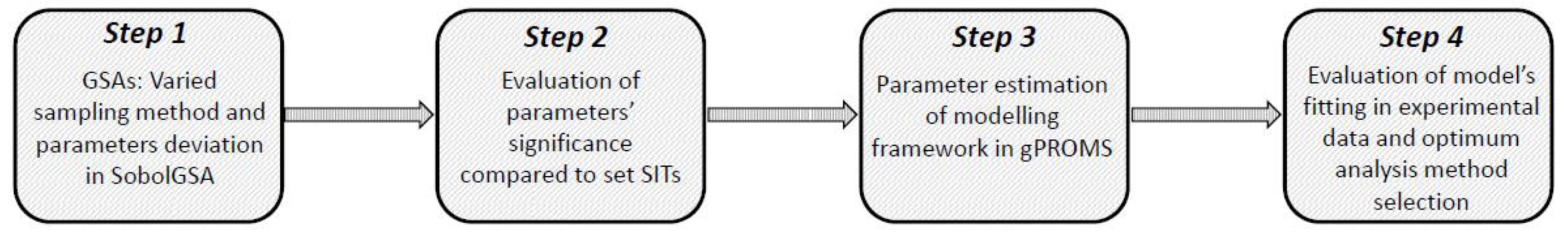
The strategic framework (Figure 1) consists of four main steps:
- Step 1:
- GSA is performed for the model in use. GSA parameters that can vary are: sampling strategy for the parameter space and metamodel building (Sobol’, Pseudo-random, Scrambled-Sobol’) and range of parameter deviation (10%, 30% and 50%).
- Step 2:
- The resulting metamodels that exhibit high agreement (R2 > 0.9) are used to progress to post-sensitivity analysis where different SITs were applied (0.05, 0.1 and 0.2) in order to indicate the significant parameters.
- Step 3:
- Each set of significant parameters indicated by Step 2 is then included in parameter estimation for the model in use.
- Step 4:
- The parameter estimation results and therefore the sensitivity analysis efficiency are subsequently evaluated in terms of goodness of fit with experimental data and the optimum analysis method is chosen.
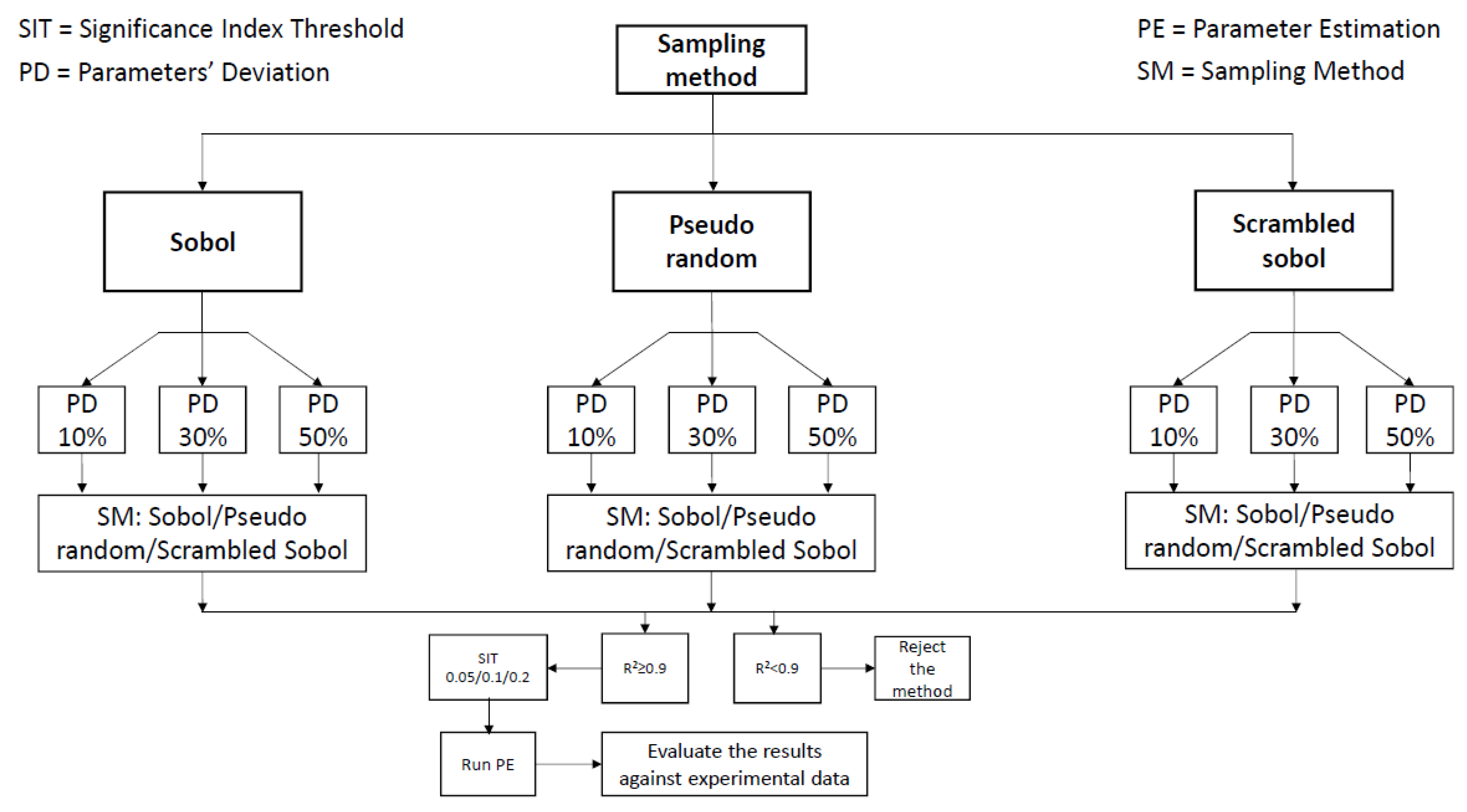
As described in Figure 1, Step 1 includes the experimentation with different parameters of the sensitivity analysis. Figure 2 describes the strategy for examining the effect of sampling method for input generation, of parameter deviation range and of the chosen SIT. As a first step, any of the three sampling methods can be chosen and the different parameter deviation values can be examined. The sampling method is used to generate 16384 (214) different groups of parameter values within the constrained—by the chosen parameters’ deviation—values space, as shown in Equation (3). Therefore, the model is simulated 16384 (214) times with the different input (parameters) sets as indicated by the chosen sampling method. Then, the different sets of sensitivity analyses—that include the construction of RS-HDMR metamodels—are performed utilizing the different sampling methods, this time for the construction of the metamodel. The sensitivity analyses that result in high metamodeling fitting are then used to perform parameter estimation using the indicated as significant parameters for each SIT.
where, is the parameter value, is the parameters’ deviation and is the nominal value of the parameter, as indicated in Table 2.
Post-analysis, the parameters that resulted in a sensitivity index higher than the SIT were regarded as significant parameters and were included in the parameter estimation. Sensitivity analysis was performed for every day of the cell culture. Due to large discrepancies of the total sensitivity index (TSI) of numerous parameters during the cell culture period and in order to evaluate the significance of the parameters for the whole time period the TSI was considered against the whole culturing period using Equation (4):
where, f(t) is the function that describes the TSI of the parameter P1 as a function of cell culture time period and SIT is the chosen threshold. If Equation (4) is satisfied, then the examined parameter is considered significant for the chosen SIT. However, the outputs considered and evaluated in the sensitivity analysis are an important factor that can substantially affect the results. For model calibration to the CHO-T cell line, the viable cell density and the extracellular antibody concentration were chosen as the outputs of interest and were considered independently. Viable cell density and antibody concentration are, to a certain extent, affected by all the other variables in the model (extracellular concentrations of metabolites and amino acids). On the other hand, during the model calibration to the GS46 cell-line, all measured variables were considered as outputs of the sensitivity analysis to additionally identify which measurements were likely to yield better estimates for each important parameter.
3. Results and Discussion
3.1. Model Calibration to CHO-T Cell Line
The model examined herein describes the cell growth, metabolism and death for the CHO-T cell line. Parameter estimation has been previously performed to fit the given experimental data and examine the predictive capabilities of the model [28]. Five of the 22 replicates of galactose and uridine feeding experiments (including the control experiment) presented significant deviation from the average behaviour of the cell line. These experiments were chosen in order to re-calibrate the model and adapt it to the unusual performance. Therefore, several sensitivity analyses methods were examined to obtain the most significant parameters of the model (Figure 2). The indicated parameters were then re-estimated and the effectiveness of the sensitivity analysis and parameter estimation was evaluated against experimental data. The emphasis was placed to the agreement of viable cell density (Xv) and antibody concentration (mAb) to experimental data and these variables were therefore used as the outputs of the sensitivity analysis. The significant parameters were re-estimated according to the feeding experiment with the lowest experimental standard deviation in terms of viable cell density and antibody concentration and their predictive capabilities were tested against the four feeding experiments with different concentrations of galactose and uridine (as well as the control). The effectiveness of the sensitivity analysis and parameter estimation was measured by the fitting of the model results to the experimental data and by the obtained 95% confidence intervals for the estimated parameters.
In order to explore the capabilities of the presented workflow, an effort to adapt the existing modeling framework to metabolic data of another cell line, named GS46 was undertaken. The metabolic data for this cell line can be found in Kyriakopoulos and Kontoravdi [33]. Model equations remained unchanged—as developed previously for the CHO-T cell line. The sensitivity analysis was performed for all 33 model parameters. Once more, the results were evaluated against the fitting of the simulation results to the experimental data and the values of the 95% confidence intervals. The parameters and their nominal values are listed in Table 2. The definition of each parameter can be found in Supplementary Material (Table S1).
3.1.1. GSA Results for the Mathematical Model
As shown in Figure 2 the sampling method (Sobol’, Scrambled-Sobol’ and Pseudo-random) and degree of parameter deviation (10%, 30% and 50%) were varied. It was not feasible to examine values over 50%, as they resulted in multiple crashes of the model during the 16384 simulations that were used for sampling. Crashes were caused due to combinations of parameters that lead to infeasible output (variables) values, e.g., negative concentration of metabolites.
The Pseudo-random sampling method resulted in R2 << 0.9 (data not shown) of metamodel fitting for all time points of the cell culture period and for both viable cell density and antibody concentration and therefore was rejected. On the other hand, both the Sobol’ and Scrambled-Sobol’ methods resulted in very high R2 >> 0.95 (data not shown) for the Xv and mAb as well and for all the different combinations of parameter deviation values and presented similar TSI for the respective parameters for both the viable cell density and the antibody concentration. The different sampling methods used for metamodel construction did not have an impact on the metamodel fit and TSI values.
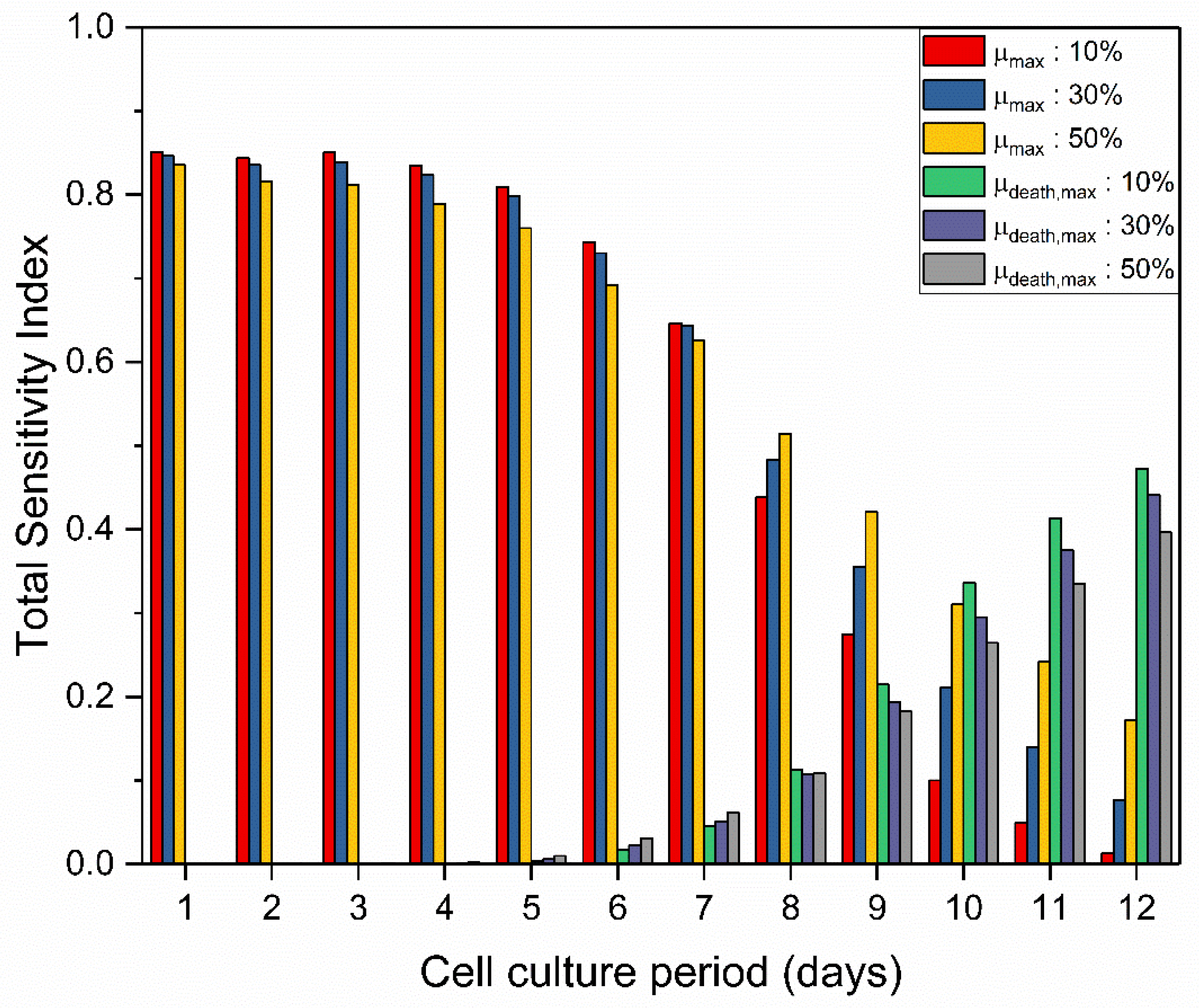
TSI values varied significantly within the cell culture time period. Figure 3 shows the variation of the TSI for the maximum specific growth rate () and the maximum specific death rate () over cell culture duration. As expected, parameters associated with cell growth and parameters associated with cell death presented higher values during the exponential and death phase respectively. resulted in a relatively constant TSI value at 0.83–0.85 until day 4, then slightly decreased until day 7 and finally presented a steep reduction until the final day of culture to a final value ranging between 0.013–0.17. On the other hand, presented low TSI values until day 7 and then started to steadily increase until the final day when it reached 0.40–0.47. Interestingly, the lower values of parameters’ deviation during sensitivity analysis resulted in higher TSI values of until day 7. However, a shift occurred in the late culture period where higher TSI values of were observed.
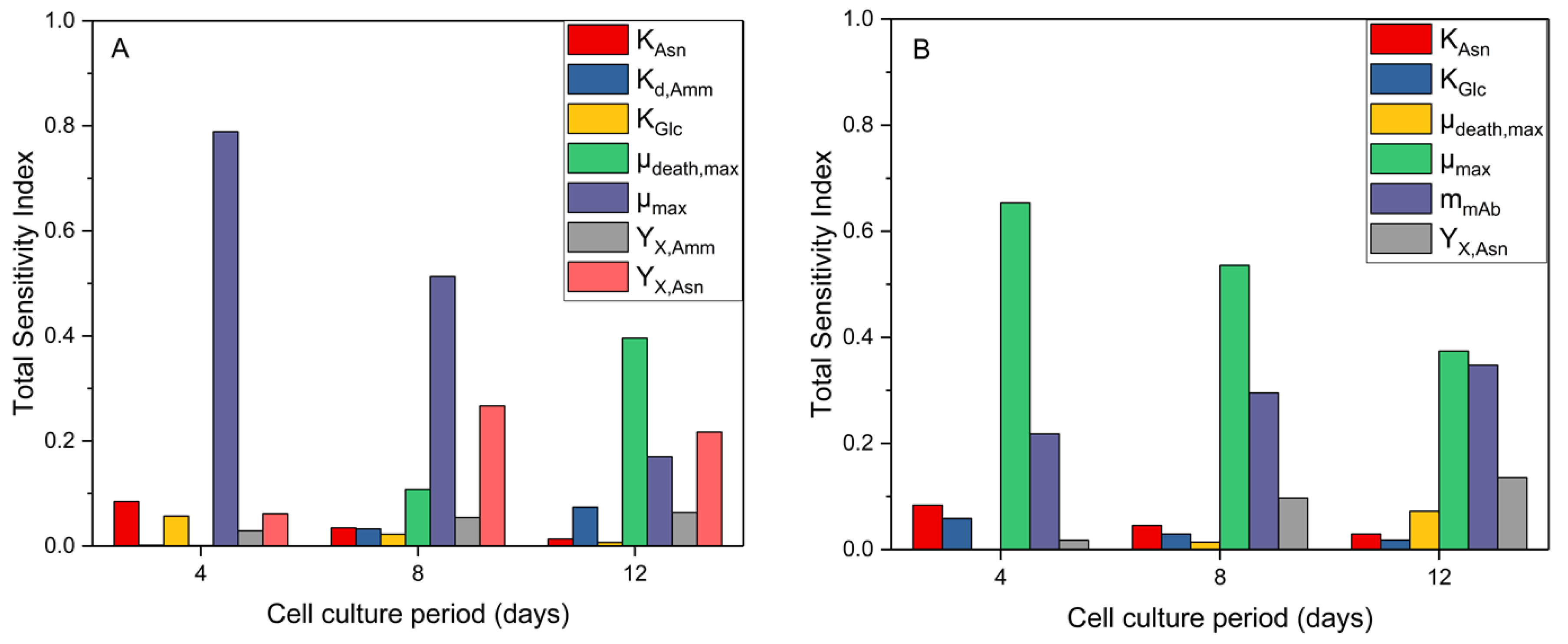
In addition, as shown in Figure 3 TSI values for different deviation ranges presented significant differences. The TSI of model parameters with values greater than 0.05 for at least one of the examined periods are shown in more detail for days 4, 8 and 12 in Figure 4. With respect to viable cell density, both and parameters present an increased TSI until the end of the cell culture. This is somewhat unsurprising considering these parameters are related to which shows the same trend. Meanwhile, the TSI of and decrease with time, probably due to the decreasing net cell growth and therefore the reduced dependence of the cell density on asparagine and glucose. Considering the impact of model parameters on antibody concentration, a significantly reduced effect of along culture time was observed, likely due to the decreasing specific growth and antibody production rates during the final days of the cell culture.
3.1.2. Post-Analysis of GSA Results and Model Calibration
In order to evaluate the results of the GSA and obtain the significant parameters, three different SIT values were examined: 0.05, 0.1 and 0.2. Considering the variation of TSI values with time, Equation (4) was used to explore the effect of each parameter during the whole cell culture period. As the TSI values between the Sobol’ and Scrambled-Sobol’ analysis methods presented comparable results (<1% discrepancy), a common analysis was performed for both methods based on the Sobol’ method. Table 3 presents all parameters that were found to exceed the SIT for each threshold. Lack of entry for any particular parameter indicates that it was not included in that parameter estimation exercise because of having been identified as not significant for that SIT. Interestingly, although the TSI and metamodeling fitting results between the three deviation percentages examined were noticeably different (Figure 3), they eventually resulted in the same set of parameters for all thresholds, indicating that although the effect of parameter deviation was observable, it was not adequate to impact the parameters that would exceed the chosen SIT in each exercise.
These reduced sets of parameters were then used to fine-tune the model to the experimental data. The results were evaluated considering the fitting to the experimental data for the FS1 feeding experiment (Figure 5) and the values of the 95% confidence intervals. FS1 was chosen for parameter estimation and model calibration as it presented the lowest experimental standard deviation in both viable cell density and antibody concentration. All estimated parameter values are presented in Table 3. Set B presented the highest R2 values (data not shown) and the narrowest 95% CI (Table 3) for all parameters. The absence of in the parameter estimation of Set B resulted in a slightly lower value of , but showed no effect on the other parameters. The more stringent SIT of 0.2 resulted in the estimation of only two parameters (Table 3), which were not adequate to successfully calibrate the model to the experimental data.
3.1.3. Model Predictive Capabilities Post Re-Calibration
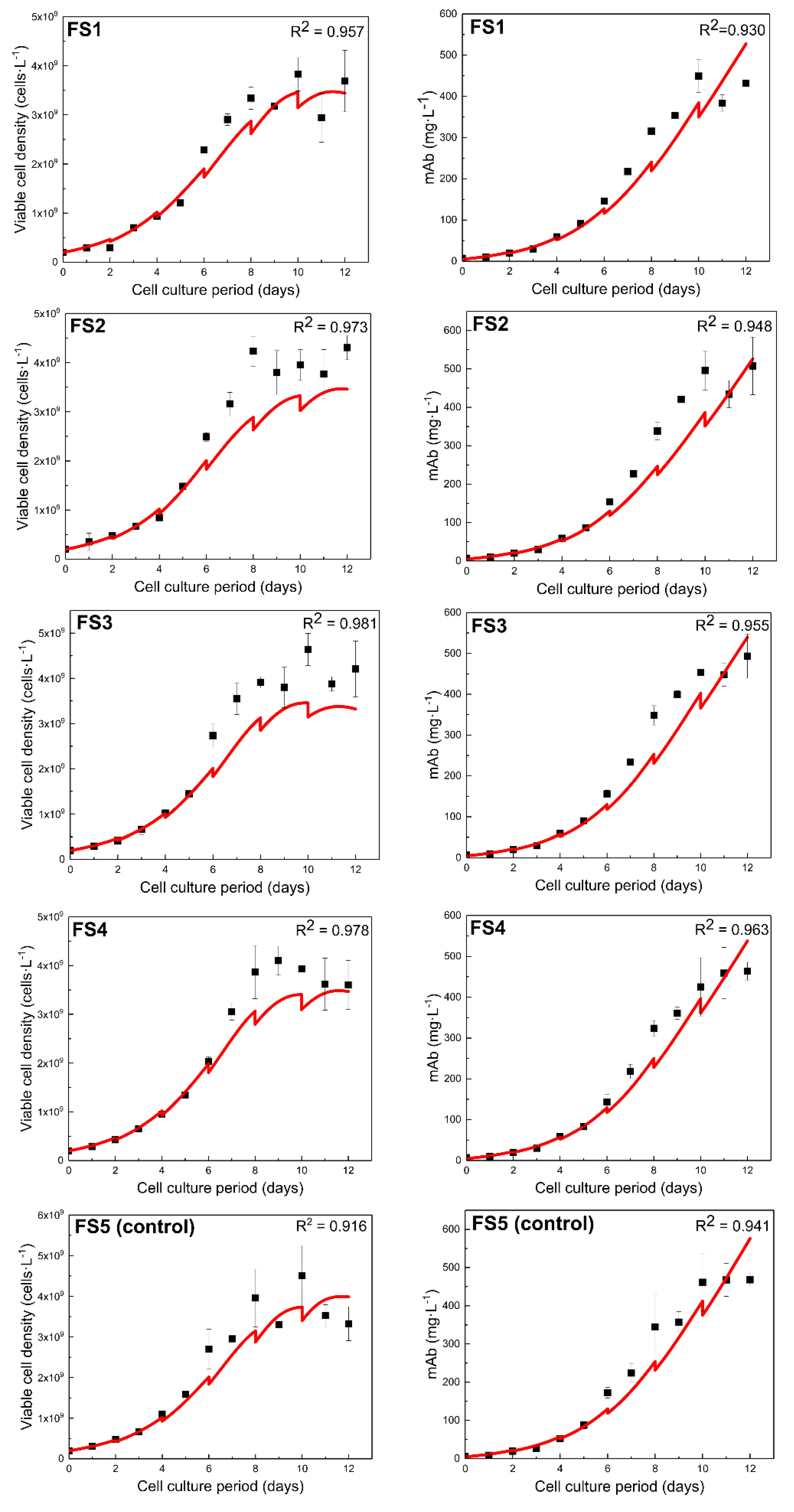
Set B parameter values were used to examine the predictive capabilities of the model in four fed-batch experiments that were not included in parameter estimation. FS2-5 experiments were used to examine the predictive capabilities of the re-calibrated model, i.e., they were not included in the parameter estimation. In brief, FS1-4 fed-batch experiments included the addition of galactose and uridine on day 4 and every other day, while FS5 was the control experiment where no galactose or uridine were added. All cultures were supplemented with CD EfficientFeedTM C AGTTM Nutrient Supplement on alternate days, starting from day 2. Model simulation (Figure 5) closely described the viable cell density of FS1 (R2 = 0.957) and the antibody concentration (R2 = 0.930) during the cell culture period.
Model fitting to all experimental data for both viable cell density and antibody concentration resulted in R2 > 0.9 (Figure 5), indicating that model re-calibration was successful. Satisfactory results were also obtained for model predictions for the remaining of the experimental feeding strategies as indicated by the R2 values for both viable cell density and antibody concentration.
3.2. Model Training to a Different CHO Cell Line (GS46)
The model was then trained to the experimental data for a second cell line, expressing a different monoclonal antibody using the workflow as described in Figure 2. Specifically, we used the experimental data for the fed-batch culture of GS46 cell line, which was grown on the same basal medium (CD-CHO) and fed with 10% v/v CD EfficientFeedTM C AGTTM Nutrient Supplement every other day starting from day 2 [33]. Galactose and uridine were not added to the cultures described in this section. The availability of complete amino acid time profiles enabled us to perform the sensitivity analysis with respect to all metabolites and certain important amino acids. Therefore, the examined outputs apart from antibody concentration included the extracellular concentrations of glucose (Glc), glutamine (Gln), ammonia (Amm), lactate (Lac), asparagine (Asn), aspartate (Asp) and glutamate (Glu). Viable cell density was not examined as an additional output due to the high correlation of this variable with the metabolite and amino acid concentrations.
The optimal sensitivity analysis settings identified in Section 3.1 were used for model calibration: Sobol’ sampling method, 50% parameter deviation around the nominal values presented in Table 1 and SIT equal to 0.1. The post-analysis evaluation was repeated for the three examined SITs in order to explore the differences in the resulting sets of significant parameters (Supplementary Material Figure S1). The sensitivity analysis, which in this case involved all measured variables as outputs, reduced the number of estimated parameters to 10 from 33. This number is more than twice the number of significant parameters in the first study (4), which is to be expected due to the larger number of outputs. The non-significant parameters were assigned to their nominal values as in Table 1. The estimated values and the 95% CI of the significant model parameters as indicated by the sensitivity analysis are presented in Table 4. The majority of estimated parameters were the yields of cell biomass on a metabolite or amino acid () with the exception of the and that were not found to significantly influence any of the examined outputs. Conversely, glucose presented a very strong dependence on and , while and showed the highest total sensitivity indices for lactate. was identified as a significant parameter for all the metabolites and amino acids, while was found to be an important parameter for glucose, glutamate, asparagine, ammonia and glutamine. However, and that resulted in high SIT with respect to viable cell density, were not found to significantly affect any of the examined outputs.
The parameter estimation was performed in sequential steps and according to the sensitivity analysis results, meaning that each parameter was estimated using the experimental data of the variables for which it was found to be significant. Briefly, , , and were calculated against the experimental measurements for asparagine, ammonia and glucose. In a second step, was estimated using the experimental measurements for glutamine, while and were fit against the lactate concentration data. , and were re-estimated using the previous estimations as initial guesses against the experimental data for glutamate, while aspartate measurements were used to estimate . The described procedure was repeated using the calculated values as initial guesses. However, in the repeated procedure the experimental measurements of viable cell density were also included in the estimation of , , and . Finally, was estimated against the experimental data for antibody concentration.
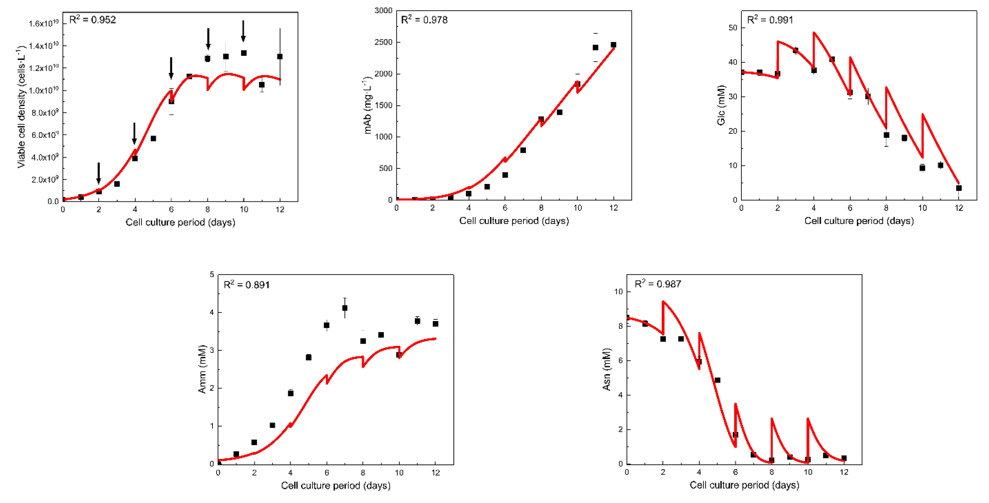
Model fitting to experimental data for viable cell density, antibody concentration, glucose, ammonia and asparagine is presented in Figure 6. Model fitting for all the variables apart from ammonia resulted in R2 > 0.95 indicating a successful tuning to the experimental data of GS46 cell line. Moreover, the R2 for ammonia was slightly lower than 0.9 (R2 = 0.891) due to the underprediction of the ammonia concentration for the biggest part of the cell culture period. Interestingly, the model was able to successfully adapt to the viable cell density and antibody concentration profile that was noticeably different than the respective profile of CHO-T. The latter achieved a peak cell density of 6 × 10⁹ cells·L−1 and 500 mg·L−1 for antibody concentration. On the other hand, GS46 significantly outperformed these numbers with the highest values reaching 1.3 × 10¹⁰ cells·L−1 and 2500 mg·L−1, respectively. The specific antibody production rates () for CHO-T and GS46 were 17.4 pg·cell−1·day−1 and 27.7 pg·cell−1·day−1, respectively. As a result, the estimated value of for the CHO-T cell line was ~44% lower that for GS46. However, the calculated presented a modest (18%) discrepancy from the respective value for the CHO-T cell line, despite the antibody concentration achieving a 5-fold higher concentration at harvest. This is due to the difference in viable cell density, which significantly enhanced the total antibody production.
4. Conclusions
The current work attempted to develop a sensitivity analysis framework that reduces the parameter estimation workload to (a) tackle problems caused in model calibration from high deviations in cell culture variables and (b) enable the calibration of a model to new datasets for different cell lines, products or culture conditions. The metabolic model used in this study was developed to describe the CHO-T fed-batch cell culture. Specifically, global sensitivity analysis was utilized to evaluate the importance of parameters (inputs) with respect to the measured variables (outputs). The impact of Sobol’, Scrambled-Sobol’ and Pseudo-random sampling methods and the deviation in parameter values by 10%, 30% or 50% on the results was evaluated. Additionally, three possible values for sensitivity index thresholds, which determine the cut-off between important and non-important parameters, namely 0.05, 0.1 and 0.2, were investigated. The Sobol’ and Scrambled-Sobol’ methods resulted in almost identical (<1% difference) metamodeling fitting and total significance indices for the examined parameters and outputs. The range of parameter value deviation was found to considerably affect the value of the significance indices, without, however, affecting the resulting sets of important parameters estimated for each SIT. The evaluation of each set of parameters was performed against experimental data for 5 different feeding strategies of galactose and uridine in fed-batch cultures and the values of the 95% confidence intervals for important parameters. The results show that estimation of parameters with a SI greater than or equal to 0.1, which in this case was four out of a total of 33 parameters, resulted in the highest R2 model fitting with experiment data, which were all above 0.916.
The optimal settings for GSA were then applied to calibrate the model to the experimental data for GS46 (presented in reference [33]). This second dataset included all amino acids as outputs of interest in the analysis of the modeling framework. The GSA indicated that ten parameters should be re-estimated in order to adapt the model to the GS46 cell line. Following a simple sequential parameter estimation strategy that was indicated by the sensitivity analysis, successful model tuning for the new cell line was achieved, acquiring also acceptable 95% confidence intervals. Model fitting resulted in R2 > 0.95 for the majority of variables. The estimated parameter values were comparable to those for the CHO-T cell line. Interestingly, the model managed to successfully describe (R2 equal to 0.952 and 0.978 respectively) both the viable cell density and antibody concentration, which showed significant discrepancies between the two cell lines. The proposed analysis and parameter estimation framework was therefore successful in systematizing the parameter estimation process for adapting the model to different conditions and for a different cell line. A considerable number of mathematical models have been proposed for different cell lines to date. Our approach demonstrates that a single modeling framework can be adopted and re-calibrated, employing the holistic framework proposed herein at a reduced workload.
Supplementary Materials
The following are available online at https://www.mdpi.com/2227-9717/7/3/174/s1, Figure S1: Correlations between the outputs (metabolites/amino acids) and the inputs (model parameters) for sensitivity index threshold set at (A) 0.05, (B) 0.1 and (C) 0.2, Table S1: Nomenclature of parameters used in the mathematical model.
Author Contributions
Conceptualization, P.K. and C.K.; methodology, P.K.; formal analysis, P.K.; resources, C.K.; data curation, P.K.; writing—original draft preparation, P.K.; writing—review and editing, P.K. and C.K.
Funding
This research received no external funding. P.K. is funded by a personal Ph.D. scholarship of the Department of Chemical Engineering, Imperial College London.
Acknowledgments
P.K. gratefully acknowledges his funding from the PhD scholarship scheme of the Department of Chemical Engineering, Imperial College London. The authors are thankful to MedImmune (Cambridge, UK) for providing the cell line used in this study.
Conflicts of Interest
The authors declare no conflict of interest.
References
- Sanderson, C.S.; Barford, J.P.; Barton, G.W. A structured, dynamic model for animal cell culture systems. Biochem. Eng. J. 1999, 3, 203–211. [Google Scholar] [CrossRef]
- Kontoravdi, C.; Asprey, S.P.; Pistikopoulos, E.N.; Mantalaris, A. Development of a dynamic model of monoclonal antibody production and glycosylation for product quality monitoring. Comput. Chem. Eng. 2007, 31, 392–400. [Google Scholar] [CrossRef]
- Nolan, R.P.; Lee, K. Dynamic model of CHO cell metabolism. Metab. Eng. 2011, 13, 108–124. [Google Scholar] [CrossRef]
- Hefzi, H.; Ang, K.S.; Hanscho, M.; Bordbar, A.; Ruckerbauer, D.; Lakshmanan, M.; Orellana, C.A.; Baycin-Hizal, D.; Huang, Y.; Ley, D. A consensus genome-scale reconstruction of Chinese hamster ovary cell metabolism. Cell Syst. 2016, 3, 434–443. [Google Scholar] [CrossRef]
- Calmels, C.; McCann, A.; Malphettes, L.; Andersen, M.R. Application of a curated genome-scale metabolic model of CHO DG44 to an industrial fed-batch process. Metab. Eng. 2019, 51, 9–19. [Google Scholar] [CrossRef] [PubMed]
- Jimenez del Val, I.; Fan, Y.; Weilguny, D. Dynamics of immature mAb glycoform secretion during CHO cell culture: An integrated modelling framework. Biotechnol. J. 2016, 11, 610–623. [Google Scholar] [CrossRef] [Green Version]
- Jedrzejewski, P.; del Val, I.; Constantinou, A.; Dell, A.; Haslam, S.; Polizzi, K.; Kontoravdi, C. Towards controlling the glycoform: A model framework linking extracellular metabolites to antibody glycosylation. Int. J. Mol. Sci. 2014, 15, 4492–4522. [Google Scholar] [CrossRef]
- Sou, S.N.; Jedrzejewski, P.M.; Lee, K.; Sellick, C.; Polizzi, K.M.; Kontoravdi, C. Model-based investigation of intracellular processes determining antibody Fc-glycosylation under mild hypothermia. Biotechnol. Bioeng. 2017, 11, 1570–1582. [Google Scholar] [CrossRef] [PubMed]
- Villiger, T.K.; Scibona, E.; Stettler, M.; Broly, H.; Morbidelli, M.; Soos, M. Controlling the time evolution of mAb N-linked glycosylation—Part II: Model-based predictions. Biotechnol. Prog. 2016, 32, 1135–1148. [Google Scholar] [CrossRef] [PubMed]
- Saltelli, A.; Annoni, P.; Azzini, I.; Campolongo, F.; Ratto, M.; Tarantola, S. Variance based sensitivity analysis of model output. Design and estimator for the total sensitivity index. Comput. Phys. Commun. 2010, 181, 259–270. [Google Scholar] [CrossRef]
- Kravaris, C.; Hahn, J.; Chu, Y. Advances and selected recent developments in state and parameter estimation. Comput. Chem. Eng. 2013, 51, 111–123. [Google Scholar] [CrossRef]
- Kiparissides, A.; Koutinas, M.; Kontoravdi, C.; Mantalaris, A.; Pistikopoulos, E.N. ‘Closing the loop’ in biological systems modeling—From the in silico to the in vitro. Automatica 2011, 47, 1147–1155. [Google Scholar] [CrossRef]
- Kontoravdi, C.; Pistikopoulos, E.N.; Mantalaris, A. Systematic development of predictive mathematical models for animal cell cultures. Comput. Chem. Eng. 2010, 34, 1192–1198. [Google Scholar] [CrossRef] [Green Version]
- Wang, Z.; Sheikh, H.; Lee, K.; Georgakis, C. Sequential parameter estimation for mammalian cell model based on in silico design of experiments. Processes 2018, 6, 100. [Google Scholar] [CrossRef]
- Kiparissides, A.; Rodriguez-Fernandez, M.; Kucherenko, S.; Mantalaris, A.; Pistikopoulos, E. Application of global sensitivity analysis to biological models. In Computer Aided Chemical Engineering; Braunschweig, B., Joulia, X., Eds.; Elsevier: Amsterdam, The Netherlands, 2008; pp. 689–694. [Google Scholar]
- Kontoravdi, C.; Asprey, S.P.; Pistikopoulos, E.N.; Mantalaris, A. Application of global sensitivity analysis to determine goals for design of experiments: An example study on antibody-producing cell cultures. Biotechnol. Prog. 2005, 21, 1128–1135. [Google Scholar] [CrossRef] [PubMed]
- Todri, E.; Amenaghawon, A.N.; Del Val, I.J.; Leak, D.J.; Kontoravdi, C.; Kucherenko, S.; Shah, N. Global sensitivity analysis and meta-modeling of an ethanol production process. Chem. Eng. Sci. 2014, 114, 114–127. [Google Scholar] [CrossRef]
- Sobol’, I.M. Global sensitivity indices for nonlinear mathematical models and their Monte Carlo estimates. Math. Comput. Simul. 2001, 55, 271–280. [Google Scholar] [CrossRef]
- Hong, H.S.; Hickernell, F.J. Algorithm 823: Implementing scrambled digital sequences. ACM Trans. Math. Softw. 2003, 29, 95–109. [Google Scholar] [CrossRef]
- Saltelli, A. Making best use of model evaluations to compute sensitivity indices. Comput. Phys. Commun. 2002, 145, 280–297. [Google Scholar] [CrossRef]
- Sobol’, I.M.; Kucherenko, S. Global sensitivity indices for nonlinear mathematical models. Review. WILMOTT Mag. 2005, 1, 56–61. [Google Scholar] [CrossRef]
- Li, G.; Rosenthal, C.; Rabitz, H. High dimensional model representations. J. Phys. Chem. A 2001, 105, 7765–7777. [Google Scholar] [CrossRef]
- Li, G.; Wang, S.-W.; Rabitz, H. Practical approaches to construct RS-HDMR component functions. J. Phys. Chem. A 2002, 106, 8721–8733. [Google Scholar] [CrossRef]
- Li, G.; Bastian, C.; Welsh, W.; Rabitz, H. Experimental design of formulations utilizing high dimensional model representation. J. Phys. Chem. A 2015, 119, 8237–8249. [Google Scholar] [CrossRef]
- Li, G.; Hu, J.; Wang, S.W.; Georgopoulos, P.G.; Schoendorf, J.; Rabitz, H. Random sampling-high dimensional model representation (RS-HDMR) and orthogonality of its different order component functions. J. Phys. Chem. A 2006, 110, 2474–2485. [Google Scholar] [CrossRef]
- Li, G.; Rabitz, H.; Yelvington, P.E.; Oluwole, O.O.; Bacon, F.; Kolb, C.E.; Schoendorf, J. Global sensitivity analysis for systems with independent and/or correlated inputs. J. Phys. Chem. A 2010, 114, 6022–6032. [Google Scholar] [CrossRef] [PubMed]
- Spiessl, S.M.; Kucherenko, S.; Becker, D.A.; Zaccheus, O. Higher-order sensitivity analysis of a final repository model with discontinuous behaviour using the RS-HDMR meta-modeling approach. Reliab. Eng. Syst. Saf. 2018. [Google Scholar] [CrossRef]
- Kotidis, P.; Jedrzejewski, P.; Sou, S.N.; Sellick, C.; Polizzi, K.; del Val, I.J.; Kontoravdi, C. Model-based optimisation of antibody galactosylation in CHO cell culture. Biotechnol. Bioeng. 2019. [Google Scholar] [CrossRef] [PubMed]
- PSE. gPROMS ModelBuilder Documentation v.5.1.1; Process Systems Enterprise Limited: London, UK, 2018. [Google Scholar]
- Kucherenko, S.; Zaccheus, O. SobolGSA Software. 2018. Available online: http://www.imperial.ac.uk/process-systems-engineering/research/free-software/sobolgsa-software/ (accessed on 20 March 2019).
- Zuniga, M.M.; Kucherenko, S.; Shah, N. Metamodelling with independent and dependent inputs. Comput. Phys. Commun. 2013, 184, 1570–1580. [Google Scholar] [CrossRef]
- Kotidis, P.; Demis, P.; Goey, C.H.; Correa, E.; McIntosh, C.; Trepekli, S.; Shah, N.; Klymenko, O.V.; Kontoravdi, C. Constrained global sensitivity analysis for bioprocess design space identification. Comput. Chem. Eng. 2019. [Google Scholar] [CrossRef]
- Kyriakopoulos, S.; Kontoravdi, C. A framework for the systematic design of fed-batch strategies in mammalian cell culture. Biotechnol. Bioeng. 2014, 111, 2466–2476. [Google Scholar] [CrossRef]
Figure 1.
Strategic framework for the evaluation of different sensitivity analysis. The framework combines sensitivity analysis in the SobolGSA software and parameter estimation in gPROMS.
Figure 1.
Strategic framework for the evaluation of different sensitivity analysis. The framework combines sensitivity analysis in the SobolGSA software and parameter estimation in gPROMS.

Figure 2.
Workflow graph for the methods used to evaluate the significant parameters.

Figure 3.
TSI values for different deviation ranges of the values for and within the cell culture time period. For all the presented sensitivity analyses Sobol’ method was used as the sampling method and viable cell density as the examined output.
Figure 3.
TSI values for different deviation ranges of the values for and within the cell culture time period. For all the presented sensitivity analyses Sobol’ method was used as the sampling method and viable cell density as the examined output.

Figure 4.
TSI for different parameters examining their effect on (A) viable cell density and (B) antibody concentration. The parameters’ deviation was set at 10% and the used sampling method was Scrambled Sobol’.
Figure 4.
TSI for different parameters examining their effect on (A) viable cell density and (B) antibody concentration. The parameters’ deviation was set at 10% and the used sampling method was Scrambled Sobol’.

Figure 5.
Model fitting (FS1) and predictions (FS2-5) to experimental data of viable cell density and antibody concentration for all the feeding strategies after parameter estimation. The R2 values for model fitting to experimental data are also shown for each experiment. Model simulations are represented by the red line and the experimental data by the black dots.

Figure 6.
Model fitting (red line) to experimental data (black dots) for the calibrated model to GS46 cell line. The fitting of the model is also evaluated by the R2 values that included in the graphs. The arrows indicate the days that the cell culture was supplemented with CD EfficientFeedTM C AGTTM Nutrient Supplement.


Table 1.
Concentrations of galactose and uridine fed to the cell culture on different days for all the experiments.
Table 1.
Concentrations of galactose and uridine fed to the cell culture on different days for all the experiments.
| Feeding Strategy | Galactose (mM) | Uridine (mM) | ||||||
|---|---|---|---|---|---|---|---|---|
| Day 4 | Day 6 | Day 8 | Day 10 | Day 4 | Day 6 | Day 8 | Day 10 | |
| FS1 | 79.35 | 15.38 | 10.99 | 248.29 | 15.87 | 3.08 | 2.20 | 49.66 |
| FS2 | 4.27 | 168.34 | 37.72 | 11.35 | 0.85 | 33.67 | 7.54 | 2.27 |
| FS3 | 5.19 | 3.11 | 235.29 | 249.94 | 1.04 | 0.62 | 47.06 | 49.99 |
| FS4 | 21.91 | 6.41 | 233.46 | 3.97 | 4.38 | 1.28 | 46.69 | 0.79 |
| FS5 (control) | - | - | - | - | - | - | - | - |
Table 2.
Model parameters that were used in the GSA and their nominal values a.
| Parameter | Value | Unit |
|---|---|---|
| μmax | 6.50 × 10⁻² | h−1 |
| μdeath,max | 1.50 × 10⁻² | h−1 |
| KGlc | 14.04 | mM |
| KAsn | 2.62 | mM |
| KIAmm | 3.17 | mM |
| KILac | 1 × 10³ | mM |
| KIUrd | 41.09 | mM |
| Kd,Amm | 14.28 | mM |
| Kd,Urd | 27.86 | mM |
| YmAb,X | 3.39 | pg·cell−1 |
| mmAb | 4.10 × 10⁻¹ | pg·cell−1·h−1 |
| 1.01 × 10⁹ | cell·mmol−1 | |
| 5.46 × 10⁷ | cell·mmol−1 | |
| 4.64 × 10⁹ | cell·mmol−1 | |
| 1.46 × 10¹⁰ | cell·mmol−1 | |
| 7.68 × 10⁸ | cell·mmol−1 | |
| 2.36 × 10⁹ | cell·mmol−1 | |
| 1.38 × 10⁸ | cell·mmol−1 | |
| 1.61 × 10⁹ | cell·mmol−1 | |
| 3.59 × 10⁹ | cell·mmol−1 | |
| 0.10 | mmol·mmol−1 | |
| 1.56 | mmol·mmol−1 | |
| 0.10 | mmol·mmol−1 | |
| 0.13 | mmol·mmol−1 | |
| 2 | mmol·mmol−1 | |
| 3.43 × 10⁻¹¹ | mmol·cell−1·h−1 | |
| 1.87 × 10⁻¹⁰ | mmol·cell−1·h−1 | |
| 5.27 | mM | |
| 0.35 | - | |
| 21.20 | mM | |
| 16 | mM | |
| 18.23 | mM | |
| 7 | mM |
a Data taken from [28].
Table 3.
Parameter estimation results for all parameter sets (A, B, C) including parameter values and their 95% confidence intervals.
Table 3.
Parameter estimation results for all parameter sets (A, B, C) including parameter values and their 95% confidence intervals.
| Set A (SIT = 0.05) | Set B (SIT = 0.1) | Set C (SIT = 0.2) | |||||
|---|---|---|---|---|---|---|---|
| Parameter | Value | 95% CI | Value | 95% CI | Value | 95% CI | Units |
| 2.66 | 0.24 | - | - | - | - | mM | |
| 1.46 × 10⁻² | 2.92 × 10⁻³ | 1.41 × 10⁻² | 2.46 × 10⁻³ | - | - | h−1 | |
| 3.89 × 10⁻² | 1.14 × 10⁻³ | 3.89 × 10⁻² | 1.14 × 10⁻³ | 3.41 × 10⁻² | 7.24 × 10⁻⁴ | h−1 | |
| 1.07 | 5.10 × 10⁻² | 1.07 | 5.10 × 10⁻² | 1.13 | 5.46 × 10⁻² | pg·cell−1·h−1 | |
| 3.46 × 10⁸ | 2.79 × 10⁷ | 3.46 × 10⁸ | 2.79 × 10⁷ | - | - | cell·mmol−1 | |
Table 4.
Estimated parameters for model adaption to GS46 cell line.
| Estimated Parameter | Value | Units | 95% Confidence Interval |
|---|---|---|---|
| 1.31 | pg·cell−1·h−1 | 1.15 × 10⁻¹ | |
| 1.06 × 10⁹ | cell·mmol−1 | 4.97 × 10⁶ | |
| 5.68 × 10⁹ | cell·mmol−1 | 8.25 × 10⁷ | |
| 18.55 | mM | 4.02 | |
| 7.14 | mM | 0.64 | |
| 1.85 × 10¹⁰ | cell·mmol−1 | 3.53 × 10⁸ | |
| 3.35 × 10⁻¹¹ | mmol·cell−1·h−1 | 3.35 × 10⁻¹² | |
| 6.96 × 10⁻² | h−1 | 6.67 × 10⁻⁴ | |
| 4.66 × 10⁹ | cell·mmol−1 | 1.67 × 10⁸ | |
| 8.69 × 10⁸ | cell·mmol−1 | 2.75 × 10⁷ |
© 2019 by the authors. Licensee MDPI, Basel, Switzerland. This article is an open access article distributed under the terms and conditions of the Creative Commons Attribution (CC BY) license (http://creativecommons.org/licenses/by/4.0/).
Share and Cite
MDPI and ACS Style
Kotidis, P.; Kontoravdi, C. Strategic Framework for Parameterization of Cell Culture Models. Processes 2019, 7, 174. https://doi.org/10.3390/pr7030174
AMA Style
Kotidis P, Kontoravdi C. Strategic Framework for Parameterization of Cell Culture Models. Processes. 2019; 7(3):174. https://doi.org/10.3390/pr7030174
Chicago/Turabian StyleKotidis, Pavlos, and Cleo Kontoravdi. 2019. "Strategic Framework for Parameterization of Cell Culture Models" Processes 7, no. 3: 174. https://doi.org/10.3390/pr7030174
Note that from the first issue of 2016, this journal uses article numbers instead of page numbers. See further details here.