Soil Mapping Based on the Integration of the Similarity-Based Approach and Random Forests


1
Key Laboratory of Virtual Geographic Environment, Nanjing Normal University, Ministry of Education, Nanjing 210023, China
2
State Key Laboratory Cultivation Base of Geographical Environment Evolution, Jiangsu Province, Nanjing 213323, China
3
Jiangsu Center for Collaborative Innovation in Geographical Information Resource Development and Application, Nanjing 210023, China
4
Department of Geography, University of Wisconsin-Madison, Madison, WI 53706, USA
5
College of Resources and Environment, University of Chinese Academy of Sciences, Beijing 100049, China
*
Author to whom correspondence should be addressed.
Land 2020, 9(6), 174; https://doi.org/10.3390/land9060174
Submission received: 23 April 2020
/
Revised: 27 May 2020
/
Accepted: 27 May 2020
/
Published: 29 May 2020
Abstract
:Digital soil mapping (DSM) is currently the primary framework for predicting the spatial variation of soil information (soil type or soil properties). Random forests and similarity-based methods have been used widely in DSM. However, the accuracy of the similarity-based approach is limited, and the performance of random forests is affected by the quality of the feature set. The objective of this study was to present a method for soil mapping by integrating the similarity-based approach and the random forests method. The Heshan area (Heilongjiang province, China) was selected as the case study for mapping soil subgroups. The results of the regular validation samples showed that the overall accuracy of the integrated method (71.79%) is higher than that of a similarity-based approach (58.97%) and random forests (66.67%). The results of the 5-fold cross-validation showed that the overall accuracy of the integrated method, similarity-based approach, and random forests range from 55% to 72.73%, 43.48% to 69.57%, and 54.17% to 70.83%, with an average accuracy of 66.61%, 57.39%, and 59.62%, respectively. These results suggest that the proposed method can produce a high-quality covariate set and achieve a better performance than either the random forests or similarity-based approach alone.
1. Introduction
Without secure soil resources, we cannot be sure of secure supplies of food, fiber, water, and the diversity of landscape [1]. Soil information is central to the rational use of soil resources and relates to the sustainability of human societies [2,3,4]. Furthermore, soil information may be used in the fields of precision agriculture, environmental change simulation, natural resource management and utilization, global change monitoring, and policy making [5,6,7,8,9]. Therefore, the acquisition of soil spatial information is of important research significance.
Digital soil mapping (DSM) is currently the primary framework for predicting the spatial distribution of soil type or other soil properties [10]. The theoretical basis of DSM is the soil-landscape concept [11], which reflects the relationships between soil information and environmental covariates. Various methods have been proposed towards DSM based on environmental covariate correlation (such as decision trees, support vector machines, random forests, and similarity-based approaches) [12,13,14,15] or spatial autocorrelation (such as simple kriging and block kriging) [16,17], or the combination of these two (such as cokriging, regression kriging, and geographically weighted regression kriging) [18,19,20]. Among these methods, the second need to meet the requirements of sample size and particular spatial distribution [17,21], the third need to meet the stationarity assumption [22]. Therefore, the first methods are widely used, of which the random forests and similarity-based methods are used widely in DSM.
The random forests approach extends to the decision trees in concept, and it is an ensemble of decision trees based on bagging predictors [23,24]. Bagging predictors is a method to generate multiple predictors and then to get an aggregated predictor [25]. The random forests approach incorporates randomness as its predictions through reiterative bootstrap sampling and randomized variable selection when generating each decision tree. Random forests has some advantages, such as the ability of modeling nonlinear and multidimensional relationships, capability of handling categorical and continuous predictors, overfitting resistance, robustness to noise features, insensitivity to missing data and outliers, unbiased measure of error rate, measure of variable importance, flexibility with various types of datasets, and high accuracy [23,26]. Despite these merits, the quality of the feature set is one of the main factors affecting the performance of random forests [27,28].
The similarity-based approach predicts soil information based on the idea that similar environmental conditions of two locations would have similar target variable values [29]. It predicts the values of the target soil property over space using the similarity measured in environmental covariate space between the prediction location and individual sample locations. The similarity-based approach is consistent with the mechanism of genesis, easy to understand and realize, capable of handling a small sample set, and can utilize the nonlinear relationship between the target variable and environmental covariate set [15]. However, the accuracy of this approach is limited by the representativeness of the soil samples [30].
To take the advantages of both the random forests and the similarity-based approach, and provide a high-quality feature set and improve the accuracy of DSM, an integrated method is proposed in this paper. The objectives of this study were to (i) present an approach for soil mapping by integrating the similarity-based approach and the random forests method; and (ii) demonstrate the ability of the developed method to map soil subgroups in comparison to the two methods before integration.
2. Study Area and Materials
2.1. Study Area
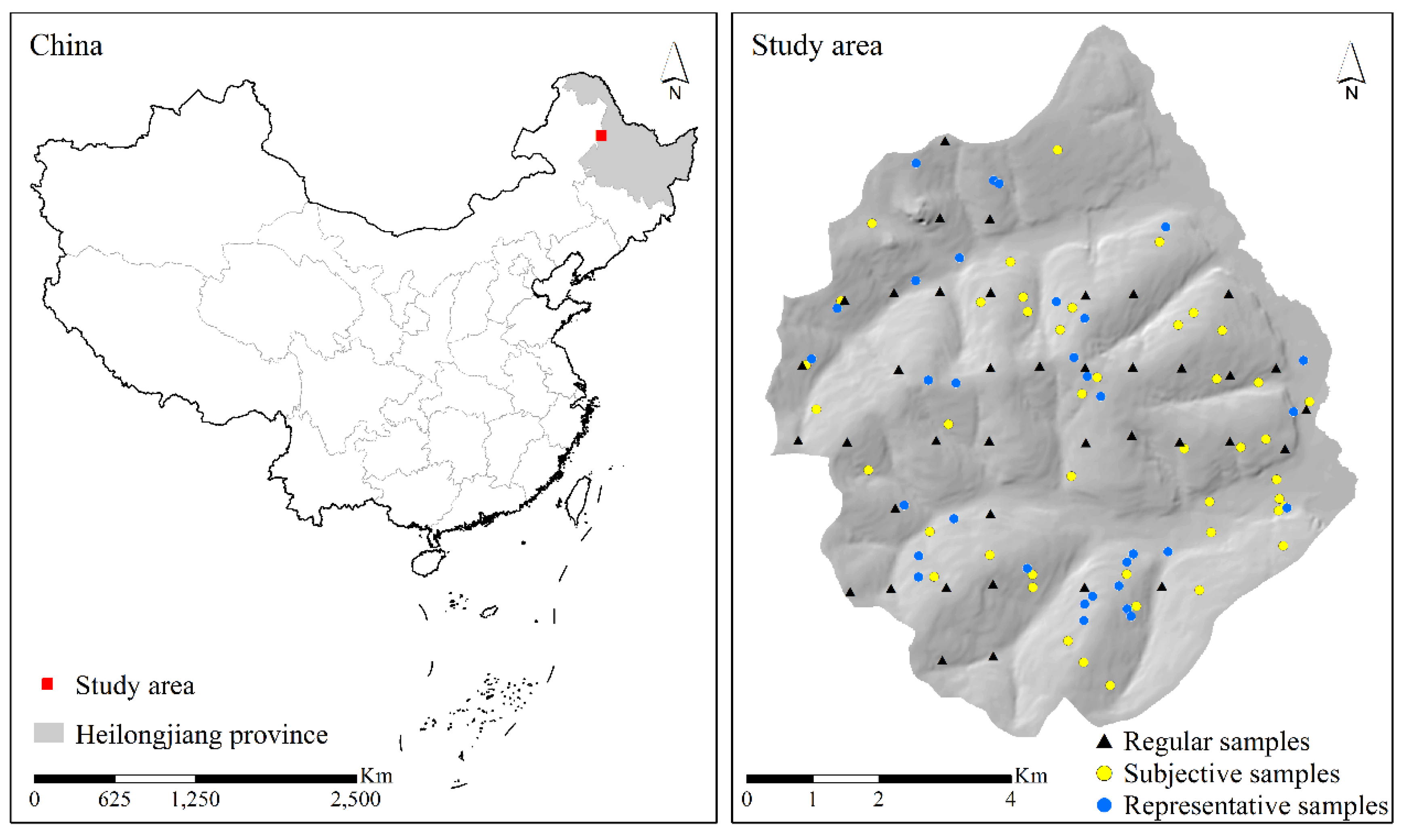
The study area is located in Heshan Farm, Nenjiang County, Heilongjiang Province, China (Figure 1). It covers an area of 60.2 km2 and is situated within longitudes 125°8′24′′ E–125°16′12′′ E and latitudes 48°53′24’’ N–48°59′24’’ N. The terrain of the area inclines from west to east. Moreover, the elevation ranges from 276 to 363 m. The area belongs to a continental monsoon climate with four seasons. The annual average temperature is about 1 to 3 °C, with a temperature range from -41 to 39 °C. The average annual precipitation ranges from 375 to 498 mm, and the average frost-free period ranges from 110 to 130 days. Besides, the accumulated temperature is 2400 to 2900 °C, which can meet the heat demand for crops. There are various kinds of crops, including wheat, soybean, corn, beet, flax, kidney bean, and potato.
2.2. Environmental Data
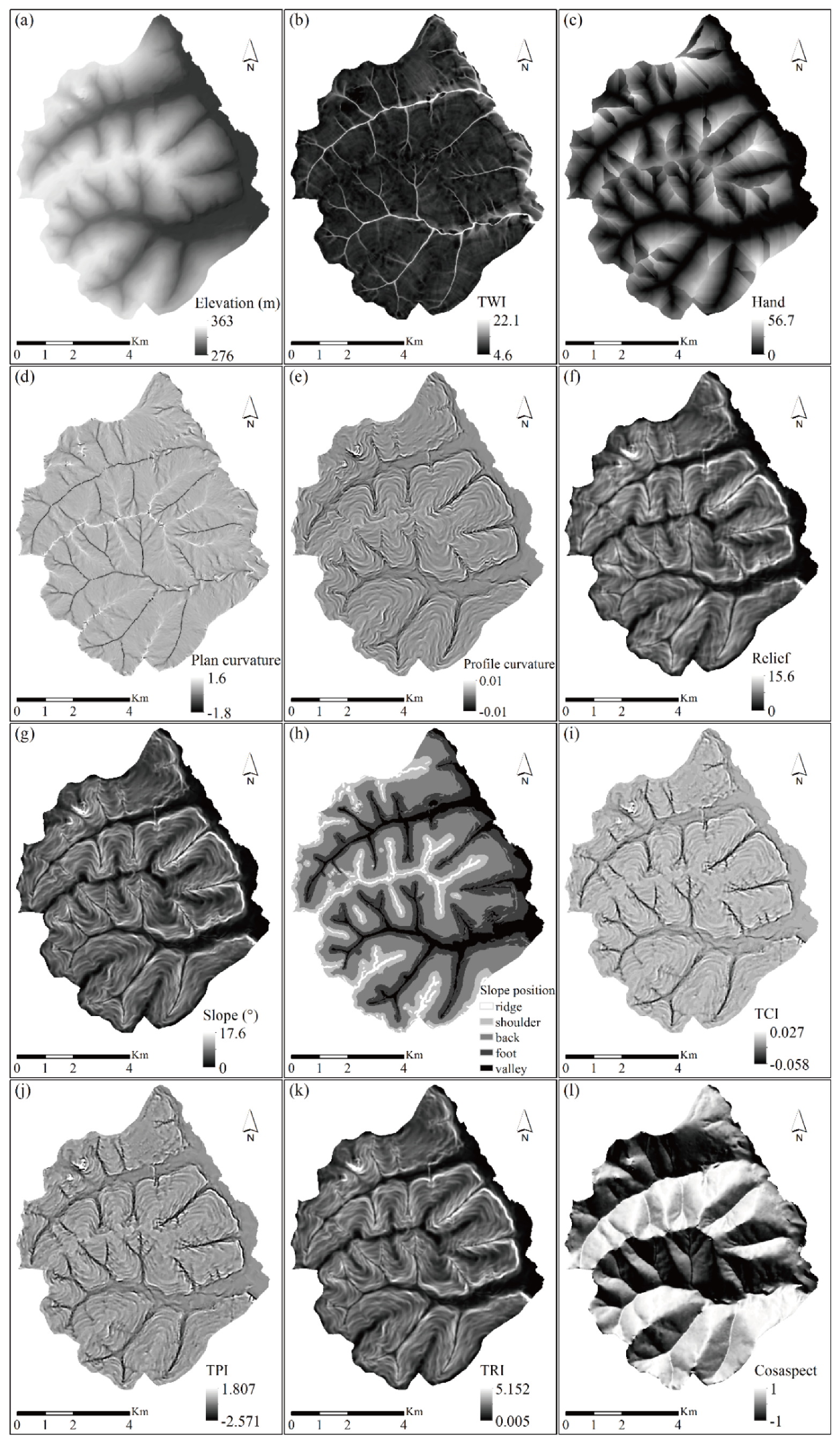
The topography is the dominant factor for spatial distribution in soils across the study area. The area is small, and its parent material and climate are generally homogeneous. A digital elevation model (DEM) with a spatial resolution of 10 m resolution was produced from a topographic map at a scale of 1:10,000. The DEM was interpolated via irregular triangular networks, which comes from contour lines in the topographic map. Based on the digital elevation model, a total of twelve environmental covariates were derived and used as follows: elevation, topographic wetness index (TWI), height above the nearest drainage (Hand), plan curvature, profile curvature, relief, slope, slope position, terrain characterization index (TCI), topographic position index (TPI), terrain ruggedness index (TRI), cosine value of the aspect (cosaspect) (Table 1, Figure 2a–l). The slope position was classified into five classes, including ridge, shoulder slope, back slope, foot slope, and valley [31].
2.3. Soil Samples
There were 115 soil samples in the study area (Figure 1). Soil samples were collected in 2005 from three sampling strategies, including integrative hierarchical stepwise sampling, subjective sampling, and systematic sampling. Thirty-two representative soil samples were collected using the integrative hierarchical stepwise sampling strategy, which aimed to collect representative samples to represent soil spatial variation by clustering environmental covariates and identifying samples based on the clustering results [30]. Slope, topographic wetness index, plan curvature, and profile curvature were used for identifying samples. Forty-four subjective samples were collected using the subjective sampling strategy, which means that experienced soil survey experts located them. Thirty-nine regular samples were collected using the systematic sampling strategy and were distributed on a grid of 1100 m (south-north direction) by 740 m (east-west direction).
The soil type of each soil sample was defined by soil experts according to soil horizons characteristics, profile properties, and Chinese soil taxonomy [40]. There are six categories in the Chinese soil classification system: order, suborder, group, subgroup, family, and series. The soil subgroup was taken as the target soil type in our study. There were six subgroups in the area: Pachic Stagni-Udic Isohumosols, Mollic Bori-Udic Cambosols, Typic Hapli-Udic Isohumosols, Typic Bori-Udic Cambosols, Lithic Udi-Orthic Primosols, and Fibric Histic-Typic Haplic Stagnic Gleyosols, which correspond to Aquic Cumulic Hapludollsy, Humic Eutrudepts, Typic Hapludolls, Typic Eutrudepts, Lithic Udorthents, and Histic Humaquepts or Typic Epiaquepts in the U.S. soil taxonomy [41].
3. Methods
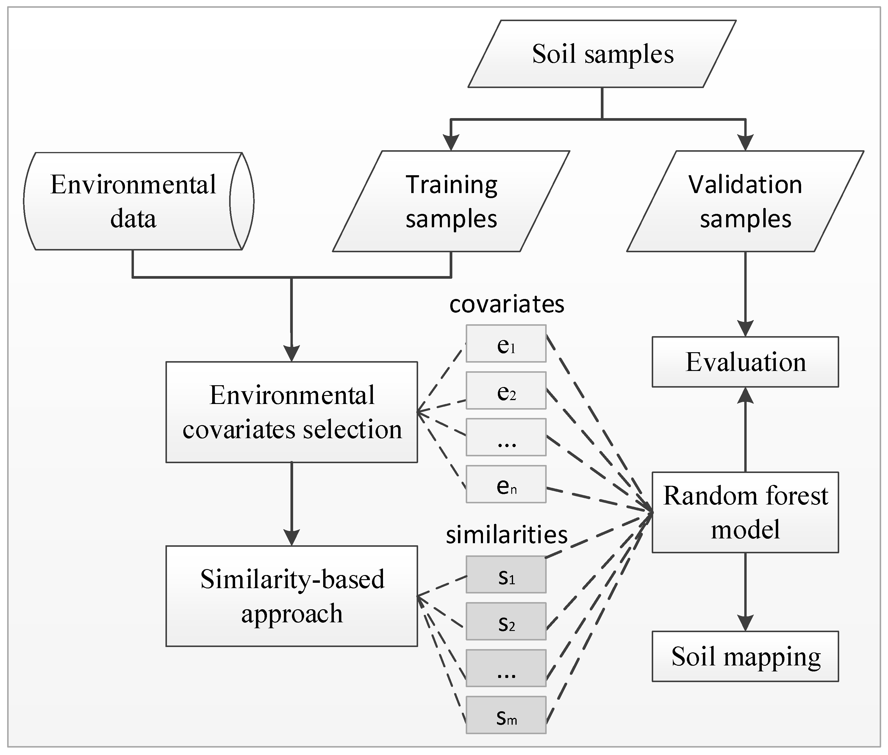
In this section, we describe the methods used in this paper. The methods include (1) Environmental covariates selection; (2) Similarity model; (3) Random forests model; (4) The integration of the similarity-based method and random forests. Finally, we lay out the experiment design for assessing the soil mapping ability of the newly developed integration model. The flowchart of the method is shown in Figure 3.
3.1. Environmental Covariates Selection
Due to the diversity of environmental covariates, it was necessary to select the covariates which are effective in mapping the variation of the targeted soil information. Environmental covariates were selected based on the importance of each covariate through the use of the random forests algorithm. The idea of assessing the significance of covariates or features in random forests is to determine how much each covariate contributes to each tree in the random forests, then take an average, and finally compare the contribution among all covariates [42]. The Gini index can measure the contribution of a covariate [43]. Gini index describes purity, similar to the meaning of information entropy; the smaller the value, the higher the purity [42]. The Scikit-Learn library [44] for Python was applied to the implementation of random forests and environmental covariates selection. For a given covariate set consisting of p covariates , the processes of covariates selection are as follows:
- (1)
- Calculate the Gini index of node m in a tree:
- (2)
- Calculate the change in the Gini index after node m is divided into m1 and m2:
- (3)
- The importance of covariate in node m is:
- (4)
- For M, a nodes set of covariate in a tree, the importance of covariate in the ith tree is:
- (5)
- The importance of covariate in the random forests composed of n trees is:
- (6)
- Normalize the importance scores of all covariates and rank the covariates according to the normalized results.
3.2. Similarity-Based Approach
The similarity-based approach assumes that locations with similar environmental conditions have similar soil types or properties [45]. Accordingly, each site in an area contains a covariate similarity vector describing how similar the site is to a set of known soil samples in a study area, with each element in the vector corresponding to a sample. The similarity value to each sample ranges from 0 to 1, with the value of 0 indicating that the environmental conditions between two locations are not similar, and the value of 1 showing that the environmental conditions between two locations are identical.
The calculation of environmental similarity between an unvisited location and a given sample is the key to the similarity-based approach. The calculation process consists of three significant steps. The first step is compilation of the environmental conditions related to the soil at each location. It is essential to employ effective covariates that can indicate the spatial variation of a targeted variable. The second step is collection of a soil sample set with the value of the target variable obtained. The third step is to calculate the similarity between each location in the study area and each of the soil samples [15]:
in which , , and denote the similarity at an unvisited location in the soil type scale, sample scale, and covariate scale, respectively. p, n, and m represent the number of soil types, samples of soil type k, and covariates, respectively, and i, j, and k signify unvisited location, sample location, and soil type, respectively. As suggested by Zhu [29], minimum and maximum functions were adopted to integrate the similarity vector. The following step equation shows the calculation of a specified categorical (e.g., parent material) or continuous (e.g., elevation) environmental covariate:
where and represent the values of the vth covariate at the location i and j. is the standard deviation of the vth covariate in the study area and is the square root of the mean deviation of the values of the vth environmental covariate at all unvisited sites from that at the sample location j. After obtaining the similarities at a location, the most appropriate soil type at the location can be inferred using the maximum operator, and the soil property can also be predicted using the similarity weighted method proposed by Zhu [29].
3.3. Random Forests
Random forests, introduced by Breiman [23], is an extended variant of bagging. Random forests is a model composed of many individual decision trees, but this model is not merely to average the prediction of all trees. The characteristics of random forests are mainly reflected in two aspects: the randomness of sampling and the randomness of feature selection [23]. The first characteristic means that each tree in a random forests model is constructed from a random sample subset. The subset is built by bootstrap sampling with replacement from the original sample set. Samples from different subsets or in the same subset can be repeated, which indicates that some samples will be used multiple times in a tree. For the second characteristic, it means that only a random subset of all the optional features are chosen when splitting each node in each tree. In other words, each splitting process of a decision tree in the random forests does not consider all the features, but randomly selects a feature subset from all the candidate features, and then selects an optimal feature from the subset for partitioning. These characteristics above can increase the diversity of decision trees in random forests, thereby improving the classification performance of the model.
The random forests algorithm consists of four main steps: (1) Select a subset from all the samples as a training set with the reiterative bootstrap sampling method; (2) Build a decision tree with the sample subset; (3) Repeat the two steps above for K times to construct K decision trees for the random forests model; and (4) Predict target variable value with the trained random forests model (multiple trees), the results of which are calculated by the prediction results of different individual trees within the forests.
The construction, training, and parameter setting of a random forests model were implemented using the Scikit-Learn Python toolkit [44]. The parameters to be optimized in random forests mainly include the number of decision trees in the forests, the maximum depth of each decision tree, the minimum number of samples required to split a node, the minimum number of samples needed to be at a leaf node, and the number of features to consider when looking for the best split. The optimal parameters of a random forests model will vary among different input samples or feature sets, so model tuning must be performed.
3.4. Integration of Similarity-Based Approach with Random Forests
The similarity-based approach and random forests are integrated by taking the outputs of a similarity-based approach as the input features of a random forests model to create the integration method. The purpose of the integration method is to take the advantages of both the similarity-based approach and random forests, provide a high-quality feature set, and improve the accuracy of digital soil mapping. The integration method is different from the similarity-based approach and random forests. The difference between the integration method and the similarity-based method lies in the digital soil mapping model itself. The difference between the random forests and the integration method lies in the feature set. The former uses the selected features only, while the latter uses the selected features and the similarity features produced by the similarity-based approach. The scale of a similarity feature set can be in the soil type scale, sample scale, or covariate scale.
3.5. Experiment Design and Evaluation
3.5.1. Experiment Design
The experiment was conducted in two ways. First, to verify the effectiveness of the integration method (SB-RF), the SB-RF is compared with the similarity-based approach (SB) and with the random forests (RF) using the selected covariates. The SB-RF, SB, and RF were used to predict soil subgroups in the study area. Since the purpose is to map the soil subgroups, the similarity features of SB-RF in the soil type scale (six similarity features in total) were used in this study. Field soil samples were divided into two parts: training samples and validation samples. The validation dataset contains 39 regular samples collected by systematic sampling. The regular samples were evenly distributed and cover most of the study area, which can objectively evaluate the results of soil mapping. The other 76 representative and subjective samples collected by integrative hierarchical stepwise and subjective sampling were used as the training dataset. Second, to reduce the impact of sampling strategies and sample size on the accuracy of each method or model, the 5-fold cross-validation was adopted for the model evaluation.
3.5.2. Evaluation
The performance of each method was evaluated using the validation samples. To estimate the prediction accuracy, a confusion matrix, and three criteria, including the overall accuracy (OA), the producer’s accuracy (PA), and the user accuracy (UA) were calculated:
where and are the number of soil types and the total number of validation samples, respectively, and , , and denote the correctly classified number, real number, and predicted number of soil type c, respectively.
4. Results and Discussion
4.1. Results of Environmental Covariates Selection
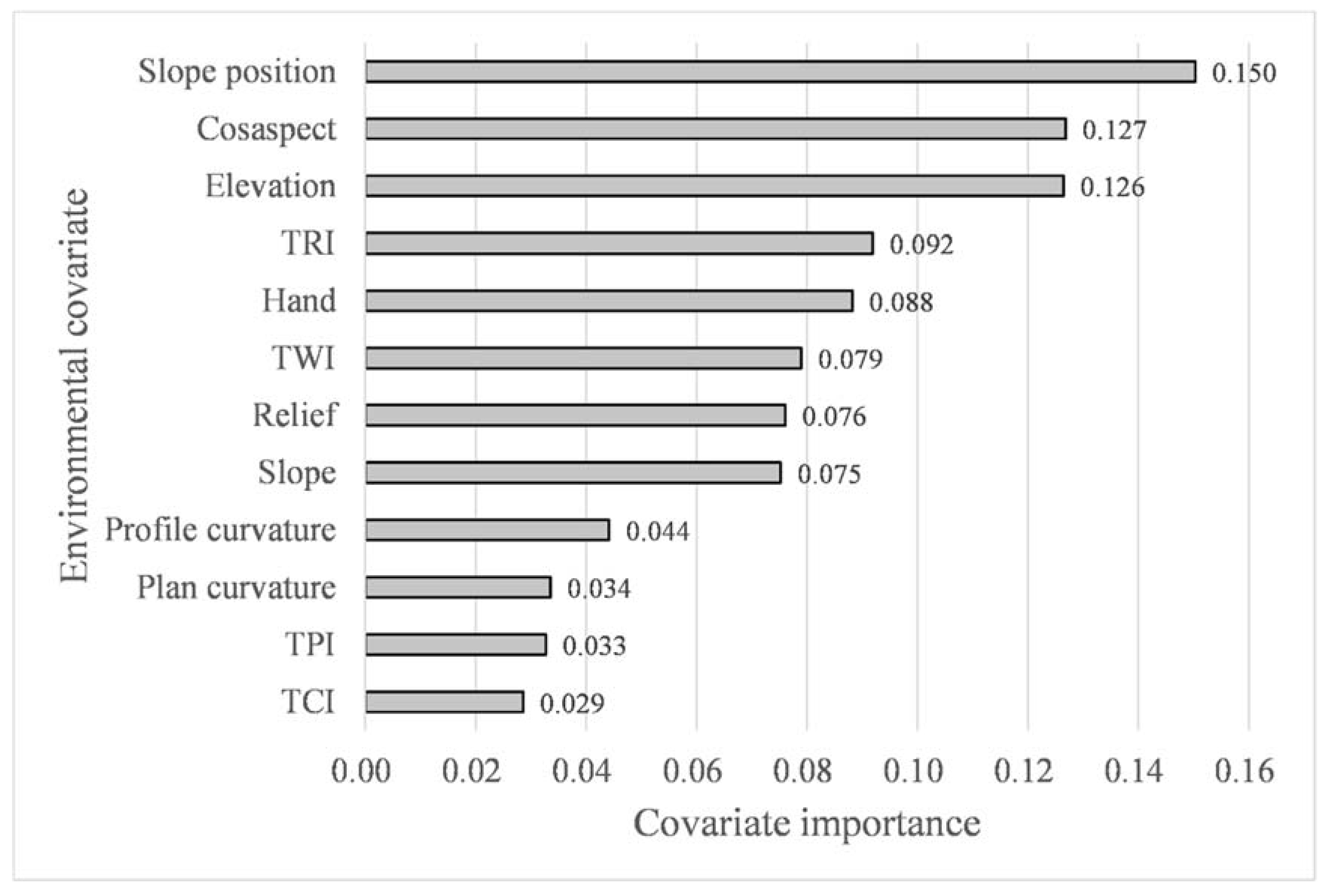
Figure 4 shows the ranked importance of environmental covariates for covariates selection. The larger the value of a covariate, the more important it is. A total of twelve factors were involved in the environmental covariates selection in this study. Out of these covariates, slope position has the highest value (0.15), followed by cosaspect (0.127), elevation (0.126), TRI (0.092), Hand (0.088), TWI (0.079), relief (0.076), and slope (0.075), respectively. Profile curvature, plan curvature, TPI, and TCI in the study area have lower covariate importance values, all of which were less than 0.05. Therefore, these four covariates were removed, and the top eight covariates with the highest importance value were selected for digital soil mapping.
4.2. Soil Mapping Results
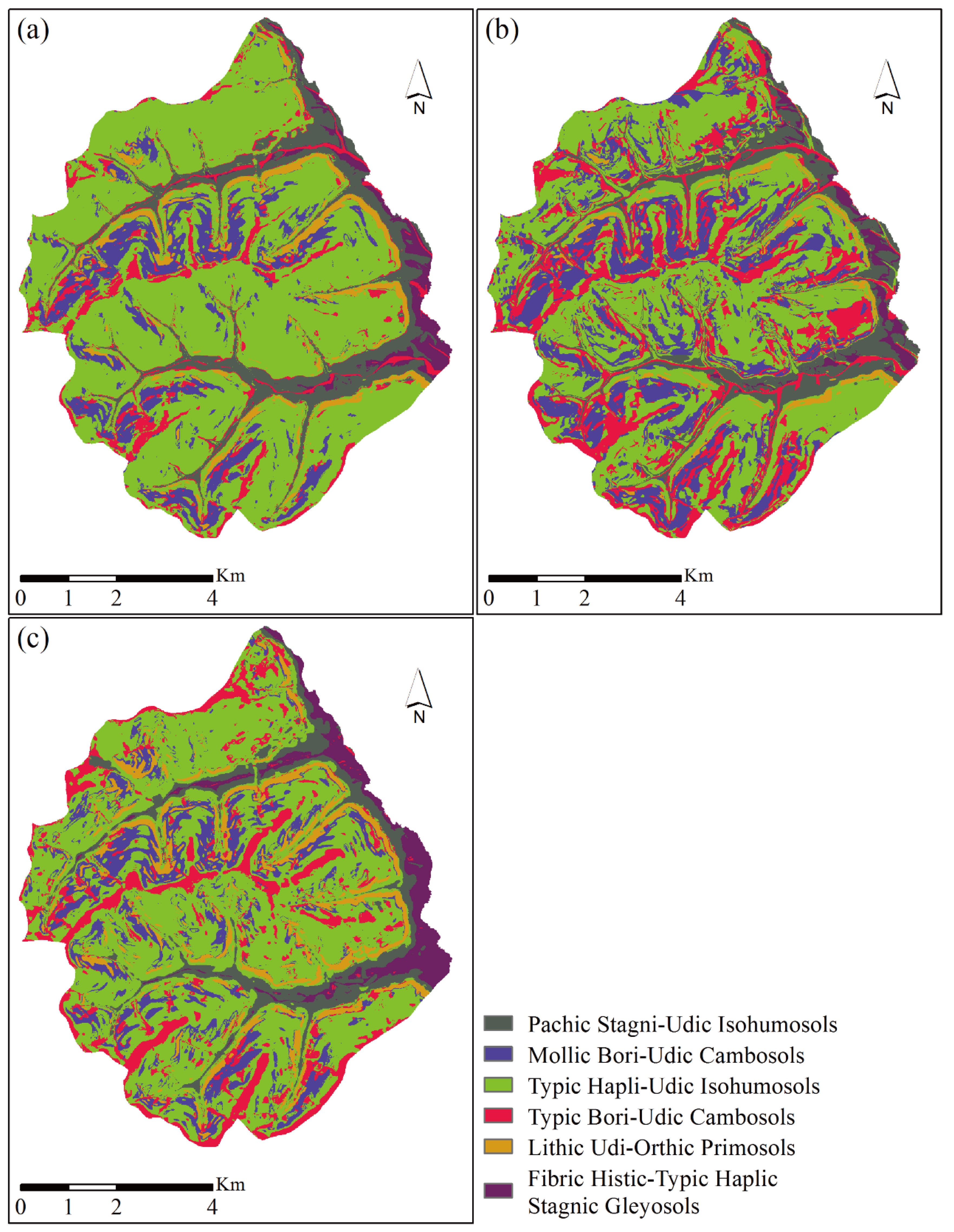
Soil mapping models, including SB-RF, SB, RF, have been constructed using 76 soil training samples. These models were used to infer the soil subgroups in the study area. The optimal parameters for SB-RF and RF in this study are shown in Table 2, which were generated by grid searching. The mapping results are shown in Figure 5a–c. The spatial distribution patterns of subgroups in soil maps generated by SB-RF, SB, and RF were different. These soil maps generated by SB, RF were more fragmented in spatial distribution than that generated by SB-RF. It is evident that Typic Hapli-Udic Isohumosols was the most widely distributed soil type in each soil map. The landform positions of soil subgroups Mollic Bori-Udic Cambosols and Typic Bori-Udic Cambosols were close, but their total area values of distribution were different. In addition, the landform positions of Pachic Stagni-Udic Isohumosols, Lithic Udi-Orthic Primosols, and Fibric Histic-Typic Haplic Stagnic Gleyosols in each map were almost the same. The comparison of mapping results and the distribution patterns of each soil subgroup indicate that the spatial distribution of subgroups in the study area was mainly affected by the mapping methods and topographic covariates.
4.3. Model Validation and Comparison
Table 3 summarizes the validation results of SB-RF, SB, and RF. As can be seen, the SB-RF method achieved the best performance for soil mapping in this study (OA = 71.79%), followed by RF (OA = 66.67%), and SB (OA = 58.97%), respectively. The results illustrate the advantage of the integration of SB and RF and demonstrate that the SB-RF method has better performance than either the RF or SB alone. The comparison between SB and RF indicates that the DSM accuracy of RF is better than that of SB under the same environmental covariates condition. Moreover, the comparison between SB-RF and RF shows that the SB-RF can achieve better performance under the same model condition, and proves that the SB approach can provide a high-quality similarity feature set for the SB-RF method.
The SB-RF model achieved the highest producer accuracy of Typic Hapli-Udic Isohumosols, followed by RF (80%) and SB (72%), respectively. Similarly, The SB-RF model achieved the highest user accuracy of Typic Hapli-Udic Isohumosols, followed by RF (71.43%) and SB (69.23%), respectively. The Typic Hapli-Udic Isohumosols soil type has the largest number of verification samples, so the validation accuracies of the SB-RF can reflect the reliability of this model. The producer accuracy of Typic Hapli-Udic Isohumosols for RF was smaller than that of SB-RF. It might be explained by the role of similarity features produced by SB. Compared with SB and RF, the SB-RF has the best producer accuracy and user accuracy for Typic Bori-Udic Cambosols, Lithic Udi-Orthic Primosols, and Fibric Histic-Typic Haplic Stagnic Gleyosols. For Pachic Stagni-Udic Isohumosols and Mollic Bori-Udic Cambosols, the producer accuracy and user accuracy of each model vary greatly. The reason for the significant difference among the producer accuracy and the user accuracy of each soil subgroup may be attributed to the difference in the sample size of each soil type. Besides, the performance of each model is also affected by the setting of model parameters, which needs to be further studied in future work.
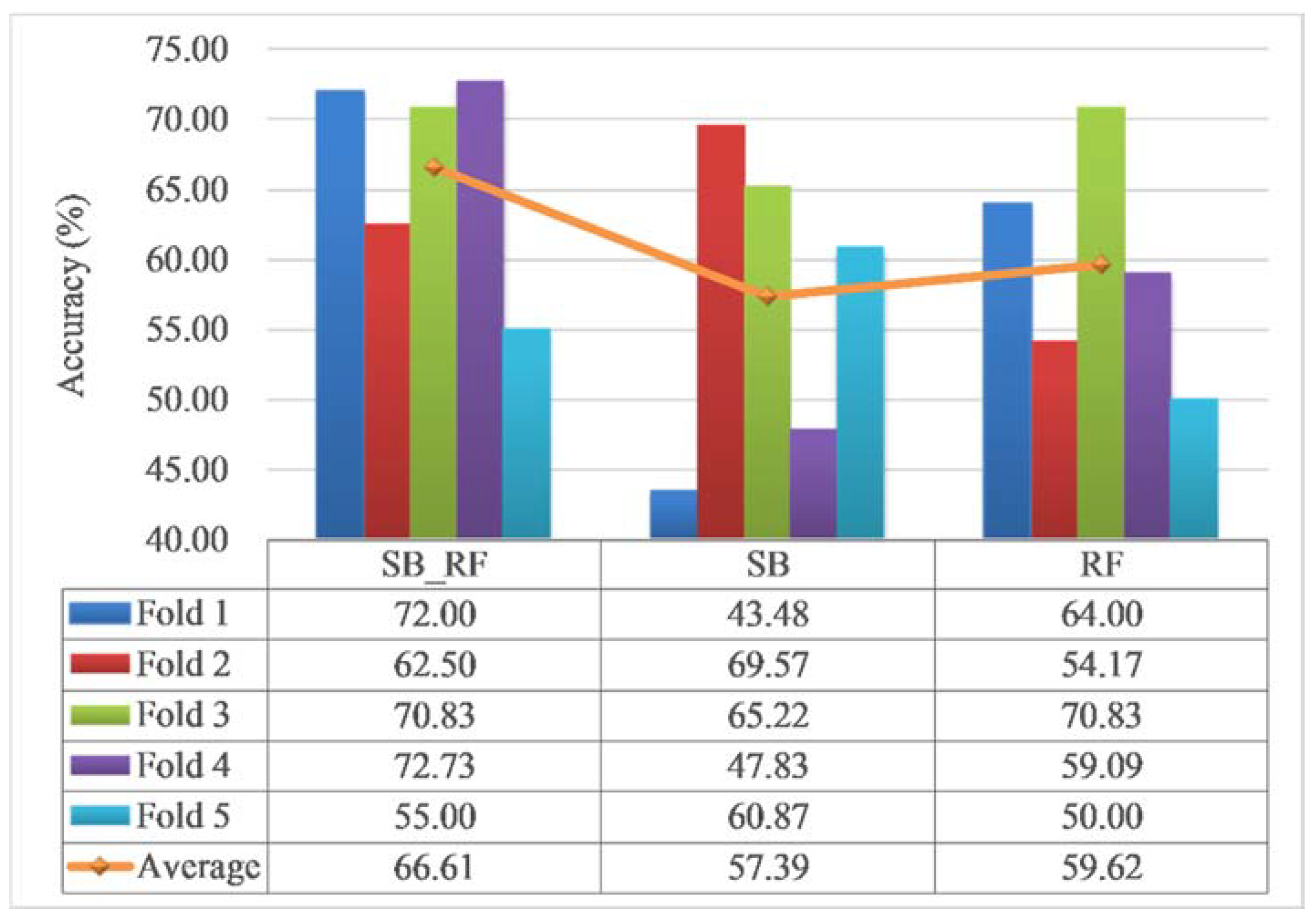
Figure 6 presents the performance of each model for the 5-fold cross-validation. It can be observed that the overall accuracies of SB-RF, SB, and RF ranged from 55% to 72.73%, 43.48% to 69.57%, and 54.17% to 70.83%, with an average accuracy of 66.61%, 57.39%, and 59.62%, respectively. The SB-RF model has a significant improvement in accuracy over the SB and RF, which shows the superiority of the integrated method again. The comparison between the RF and SB-RF demonstrates the effectiveness of the similarity feature set. In general, the accuracy of each model in the case using 5-fold cross-validation, compared with the case using regular samples as the validation dataset, has changed notably. However, the research can still prove the superiority and effectiveness of the proposed integration method.
4.4. Effectiveness of the Similarity Covariates
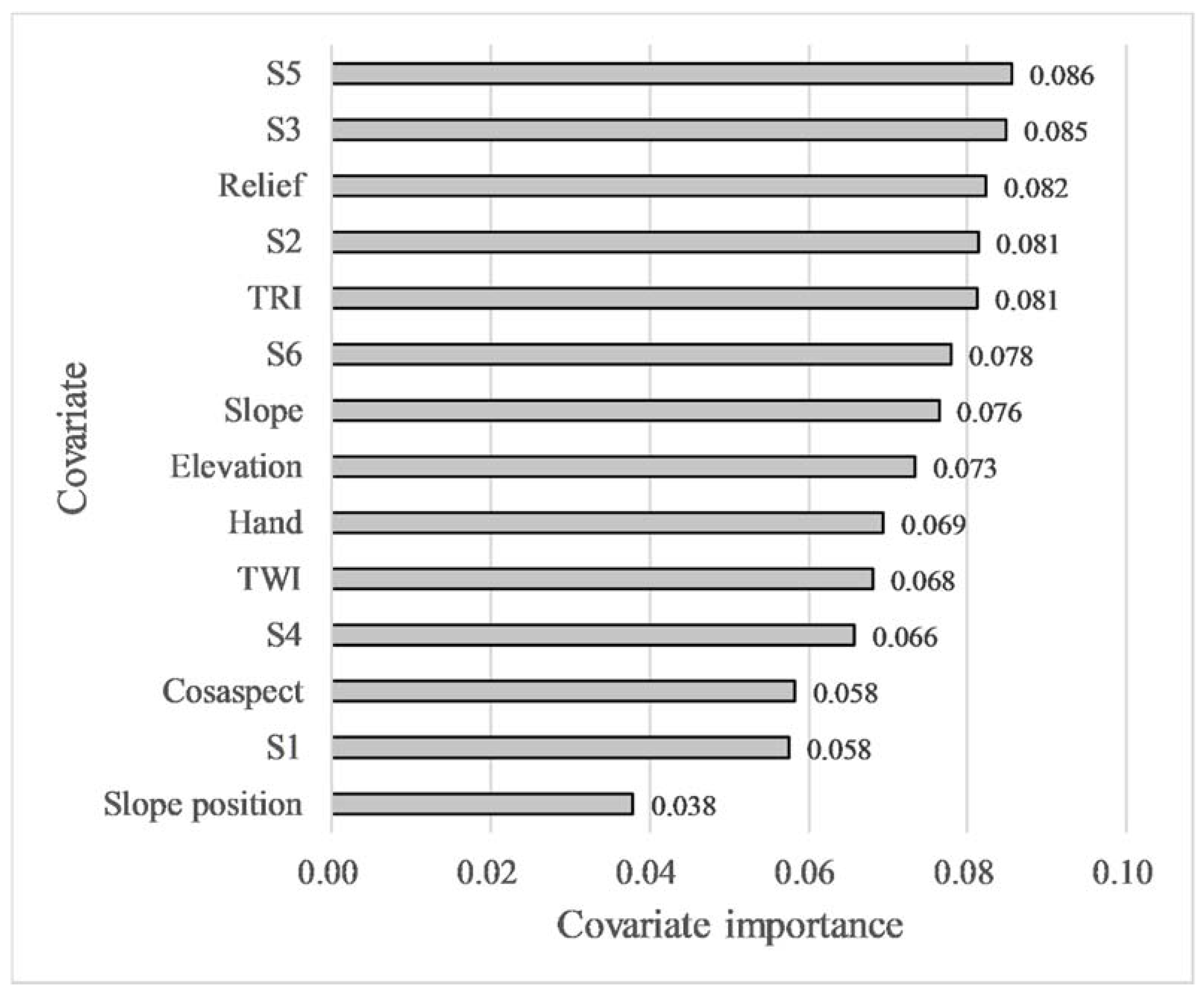
Figure 7 exhibits the importance ranking of covariates in the SB-RF model. A total of fourteen covariates, including eight selected environmental covariates and similarity covariates of six soil subgroups (S1, S2, S3, S4, S5, S6), were involved in the calculation of covariate importance. The S5 achieved the best covariate importance value (0.086), followed by S3 (0.085), relief (0.082), S2 (0.081), TRI (0.081), S6 (0.078), slope (0.076), elevation (0.073), Hand (0.069), TWI (0.068), S4 (0.066), cosaspect (0.058), S1 (0.058), and slope position (0.038), respectively. Compared with the results of covariates selection, the importance ranking of covariates has changed considerably after adding six similarity covariates. Similarity covariates occupied four of the top ten most important covariates, and S1 and S2 were the top two. The results indicate the importance and value of the similarity covariates.
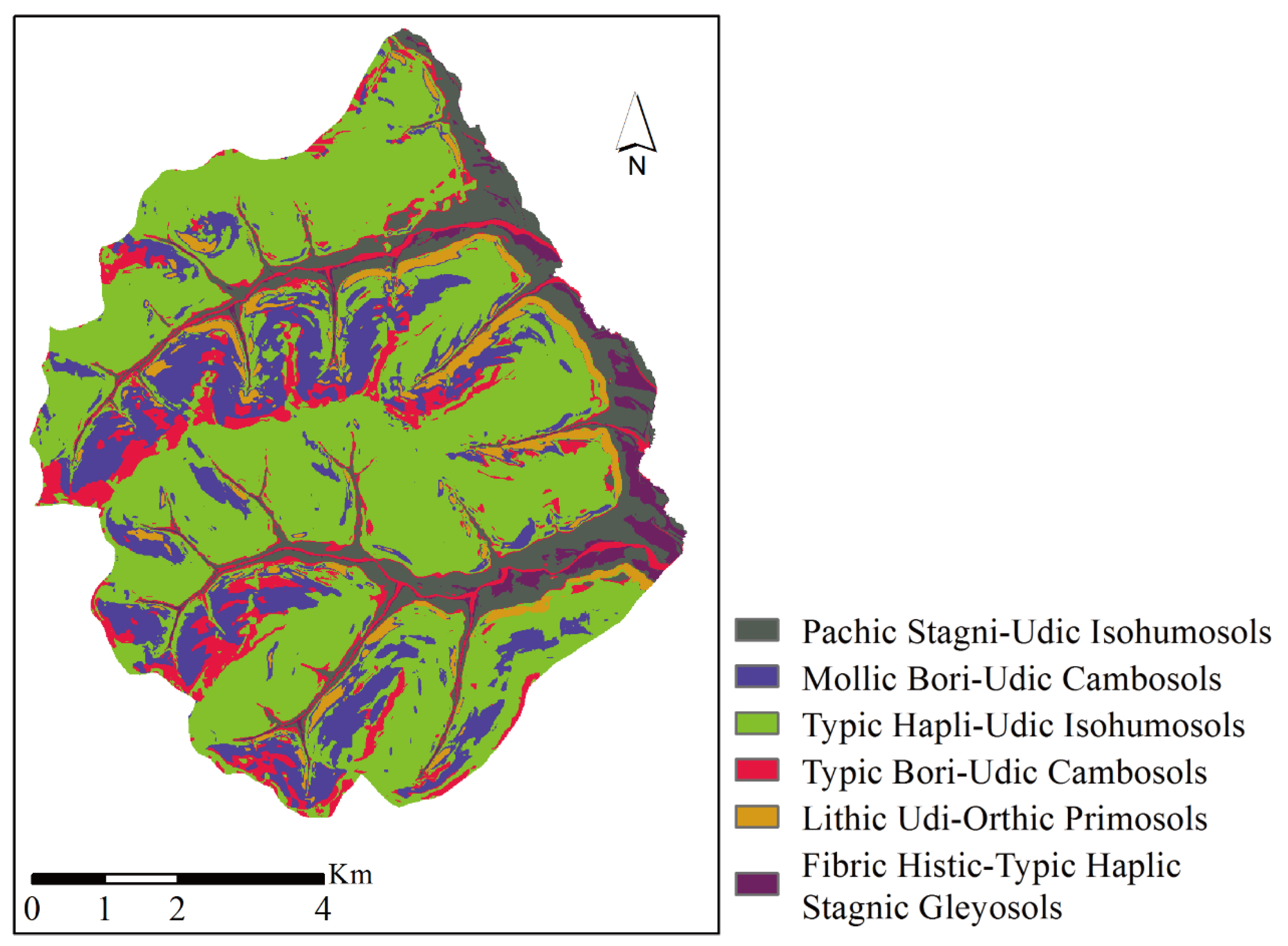
Figure 8 shows the predicted map generated by the RF model with soil type similarities as features only. The overall accuracy of the map is 66.67%, which is equal to the accuracy of the RF model with environmental covariates. The average accuracy of the 5-fold cross-validation of the map is 58.72%, which is close to the accuracy of the RF model with environmental covariates of 59.62%. In addition, the spatial distribution patterns of subgroups in the map are similar to the map generated by SB-RF. Based on the comparison above, we can conclude that the modeling accuracy of similarity features is close to that of environmental covariates. Due to the number of similarity features being less than that of environmental covariates, we indicate that the similarity features are more refined.
4.5. Impact of the Sampling Strategy and the Quality of Soil Samples
To explore the impact of sampling strategies on the performance of the SB-RF method, three SB-RF models were trained with a sample set in different sampling strategies, respectively. Choosing any one for modeling, the other two for verifying the accuracy of the model, repeating the experiment five times can get the results as shown in Table 4. The overall accuracy of SB-RF based on representative, regular, and subjective samples ranges from 63.86% to 66.27%, 47.37% to 52.63%, and 63.38% to 64.79%, with an average accuracy of 65.31%, 49.21%, and 64.23%, respectively. The accuracy of the SB-RF based on regular samples is significantly lower than that of representative and subjective samples. The model accuracy of the representative samples is slightly higher than that of subjective samples. The comparison of different model accuracy shows that the sampling strategy affects the accuracy of the SB-RF model.
The quality of soil samples can affect not only the accuracy of the SB-RF model, but also the evaluation of the prediction of the model. Previous studies have shown that the uncertainty of evaluation results change with the location and number of validation samples [46]. In this study, soil mapping results were evaluated by the regular samples. However, in the process of sample collection, the location of the collected sample set is different from the designed sample set due to the positioning error or the accessibility of the target sample. Consequently, the collected regular samples do not appear to fit a strictly regular distribution over the study area, which will increase the uncertainty of evaluation results.
4.6. Applicability and Limitations of the Integrated Approach
The case study showed that the proposed method can effectively take the advantages of both the similarity-based approach and random forests, provide a high-quality feature set, and achieve high accuracy in predicting soil types. Besides the advantages, there are limitations in the method proposed in this paper. First, the integrated method examined only a small area for mapping soil types. Second, the parameter optimization of the model is time-consuming. Third, there are many ways to select features. Different methods get different feature sets. How to select feature sets and the influence of feature selection methods on model accuracy need further study. The integration of DSM methods is a trend. Besides the integration of the similarity-based method and random forests, the integration of other methods (such as a tree-based model and neural network model) is also worth further study.
5. Conclusions
This paper presented a method for soil mapping by integrating the similarity-based approach and random forests. The presented method was applied to the Heshan study area to verify its effectiveness. The following conclusions can be drawn from this study: (1) The SB-RF method achieved a better performance in accuracy than either the RF or SB alone, which shows the effectiveness and superiority of the integrated method; (2) The similarity covariates produced by the similarity-based approach embedded valuable information, which can effectively improve the mapping accuracy. The sampling strategy affects the accuracy of the SB-RF method.
Author Contributions
Funding acquisition, A.-X.Z.; Methodology, D.W.; Writing—original draft, D.W.; Writing—review & editing, A.-X.Z. All authors have read and agreed to the published version of the manuscript.
Funding
This research was funded by grants from the National Natural Science Foundation of China (Project No.: 41871300, 41431177), the National Basic Research Program of China (Project No.: 2015CB954102), PAPD, and Outstanding Innovation Team in Colleges and Universities in Jiangsu Province. The APC was funded by the National Basic Research Program of China (Project No.: 2015CB954102).
Acknowledgments
This study was supported by grants from the National Natural Science Foundation of China (Project No.: 41871300, 41431177), the National Basic Research Program of China (Project No.: 2015CB954102), PAPD, and Outstanding Innovation Team in Colleges and Universities in Jiangsu Province. Supports to A-Xing Zhu through the Vilas Associate Award, the Hammel Faculty Fellow Award, and the Manasse Chair Professorship from the University of Wisconsin-Madison are greatly appreciated.
Conflicts of Interest
The authors declare no conflict of interest.
References
- McBratney, A.; Field, D.J.; Koch, A. The dimensions of soil security. Geoderma 2014, 213, 203–213. [Google Scholar] [CrossRef] [Green Version]
- Nauman, T.W.; Thompson, J.A.; Rasmussen, C. Semi-Automated Disaggregation of a Conventional Soil Map Using Knowledge Driven Data Mining and Random Forests in the Sonoran Desert, USA. Photogramm. Eng. Remote Sens. 2014, 80, 353–366. [Google Scholar] [CrossRef]
- Keesstra, S.D.; Bouma, J.; Wallinga, J.; Tittonell, P.; Smith, P.; Cerda, A.; Montanarella, L.; Quinton, J.N.; Pachepsky, Y.; van der Putten, W.H.; et al. The significance of soils and soil science towards realization of the United Nations Sustainable Development Goals. Soil 2016, 2, 111–128. [Google Scholar] [CrossRef] [Green Version]
- Bouma, J. Reaching out from the soil-box in pursuit of soil security. Soil Sci. Plant Nutr. 2015, 61, 556–565. [Google Scholar] [CrossRef] [Green Version]
- Minasny, B.; McBratney, A.B. Digital soil mapping: A brief history and some lessons. Geoderma 2016, 264, 301–311. [Google Scholar] [CrossRef]
- Petersen, C. Precision gps navigation for improving agricultural productivity. GPS World 1991, 2, 38–44. [Google Scholar]
- MacMillan, R.A.; Moon, D.E.; Coupe, R.A. Automated predictive ecological mapping in a forest region of BC, Canada, 2001–2005. Geoderma 2007, 140, 353–373. [Google Scholar] [CrossRef]
- Zhang, G.-L.; Liu, F.; Song, X.-D. Recent progress and future prospect of digital soil mapping: A review. J. Integr. Agric. 2017, 16, 2871–2885. [Google Scholar] [CrossRef]
- Bouma, J.; Broll, G.; Crane, T.A.; Dewitte, O.; Gardi, C.; Schulte, R.P.O.; Towers, W. Soil information in support of policy making and awareness raising. Curr. Opin. Environ. Sustain. 2012, 4, 552–558. [Google Scholar] [CrossRef]
- McBratney, A.B.; Santos, M.M.; Minasny, B. On digital soil mapping. Geoderma 2003, 117, 3–52. [Google Scholar] [CrossRef]
- Jenny, H. Factors of Soil Formation: A System of Quantitative Pedology; Dover Publications: New York, NY, USA, 1941. [Google Scholar]
- Henderson, B.L.; Bui, E.N.; Moran, C.J.; Simon, D. Australia-wide predictions of soil properties using decision trees. Geoderma 2005, 124, 383–398. [Google Scholar] [CrossRef]
- Kovačević, M.; Bajat, B.; Gajić, B. Soil type classification and estimation of soil properties using support vector machines. Geoderma 2010, 154, 340–347. [Google Scholar] [CrossRef]
- Heung, B.; Bulmer, C.E.; Schmidt, M.G. Predictive soil parent material mapping at a regional-scale: A Random Forest approach. Geoderma 2014, 214, 141–154. [Google Scholar] [CrossRef]
- Zhu, A.-X.; Liu, J.; Du, F.; Zhang, S.j.; Qin, C.Z.; Burt, J.; Behrens, T.; Scholten, T. Predictive soil mapping with limited sample data. Eur. J. Soil Sci. 2015, 66, 535–547. [Google Scholar] [CrossRef]
- Li, J.; Heap, A.D. A review of comparative studies of spatial interpolation methods in environmental sciences: Performance and impact factors. Ecol. Inform. 2011, 6, 228–241. [Google Scholar] [CrossRef]
- Li, J.; Heap, A.D. Spatial interpolation methods applied in the environmental sciences: A review. Environ. Model. Softw. 2014, 53, 173–189. [Google Scholar] [CrossRef]
- Odeh, I.O.A.; McBratney, A.B.; Chittleborough, D.J. Further results on prediction of soil properties from terrain attributes: Heterotopic cokriging and regression-kriging. Geoderma 1995, 67, 215–226. [Google Scholar] [CrossRef]
- Mondal, A.; Khare, D.; Kundu, S.; Mondal, S.; Mukherjee, S.; Mukhopadhyay, A. Spatial soil organic carbon (SOC) prediction by regression kriging using remote sensing data. Egypt. J. Remote Sens. Space Sci. 2017, 20, 61–70. [Google Scholar] [CrossRef] [Green Version]
- Kumar, S.; Lal, R.; Liu, D. A geographically weighted regression kriging approach for mapping soil organic carbon stock. Geoderma 2012, 189–190, 627–634. [Google Scholar] [CrossRef]
- Brus, D.J.; Heuvelink, G.B.M. Optimization of sample patterns for universal kriging of environmental variables. Geoderma 2007, 138, 86–95. [Google Scholar] [CrossRef]
- Zhu, A.X.; Lu, G.; Liu, J.; Qin, C.Z.; Zhou, C. Spatial prediction based on Third Law of Geography. Annals of GIS 2018, 24, 1–16. [Google Scholar] [CrossRef]
- Breiman, L. Random forests. Mach. Learn. 2001, 45, 5–32. [Google Scholar] [CrossRef] [Green Version]
- Cutler, D.R.; Edwards, T.C., Jr.; Beard, K.H.; Cutler, A.; Hess, K.T.; Gibson, J.; Lawler, J.J. Random forests for classification in ecology. Ecology 2007, 88, 2783–2792. [Google Scholar] [CrossRef] [PubMed]
- Breiman, L. Bagging predictors. Mach. Learn. 1996, 24, 123–140. [Google Scholar] [CrossRef] [Green Version]
- Liaw, A.; Wiener, M. Classification and regression by randomForest. R News 2002, 2, 18–22. [Google Scholar]
- Grunwald, S. Multi-criteria characterization of recent digital soil mapping and modeling approaches. Geoderma 2009, 152, 195–207. [Google Scholar] [CrossRef]
- Hua, J.P.; Xiong, Z.X.; Lowey, J.; Suh, E.; Dougherty, E.R. Optimal number of features as a function of sample size for various classification rules. Bioinformatics 2005, 21, 1509–1515. [Google Scholar] [CrossRef] [Green Version]
- Zhu, A.-X. A similarity model for representing soil spatial information. Geoderma 1997, 77, 217–242. [Google Scholar] [CrossRef]
- Yang, L.; Zhu, A.-X.; Qi, F.; Qin, C.-Z.; Li, B.; Pei, T. An integrative hierarchical stepwise sampling strategy for spatial sampling and its application in digital soil mapping. Int. J. Geogr. Inf. Sci. 2013, 27, 1–23. [Google Scholar] [CrossRef]
- Qin, C.Z.; Shi, X.; Li, B.L.; Pei, T.; Zhou, C.H. Quantification of spatial gradation of slope positions. Geomorphology 2009, 110, 152–161. [Google Scholar] [CrossRef]
- Qin, C.-Z.; Pei, T.; Li, B.-L.; Scholten, T.; Behrens, T.; Zhou, C.-H. An approach to computing topographic wetness index based on maximum downslope gradient. Precis. Agric. 2011, 12, 32–43. [Google Scholar] [CrossRef]
- Qin, C.-Z.; Lu, Y.; Bao, L.; Qiu, W.; Cheng, W. Simple Digital Terrain Analysis Software (SimDTA 1.0) and Its Application in Fuzzy Classification of Slope Positions. Geo-inf. Sci. 2009, 11, 737–743. [Google Scholar] [CrossRef]
- Gharari, S.; Hrachowitz, M.; Fenicia, F.; Savenije, H.H.G. Hydrological landscape classification: Investigating the performance of HAND based landscape classifications in a central European meso-scale catchment. Hydrol. Earth Syst. Sci. 2011, 15, 3275–3291. [Google Scholar] [CrossRef] [Green Version]
- Shary, P.A.; Sharaya, L.S.; Mitusov, A.V. Fundamental quantitative methods of land surface analysis. Geoderma 2002, 107, 1–32. [Google Scholar] [CrossRef]
- Skidmore, A.K. Terrain position as mapped from a gridded digital elevation model. Int. J. Geogr. Inf. Syst. 1990, 4, 33–49. [Google Scholar] [CrossRef]
- Park, S.J.; van de Giesen, N. Soil-landscape delineation to define spatial sampling domains for hillslope hydrology. J. Hydrol. 2004, 295, 28–46. [Google Scholar] [CrossRef]
- Weiss, A. Topographic position and landforms analysis. In Proceedings of the Poster Presentation, ESRI User Conference, San Diego, CA, USA, 9–13 July 2001. [Google Scholar]
- Riley, S.; Degloria, S.; Elliot, S.D. A Terrain Ruggedness Index that Quantifies Topographic Heterogeneity. Int. J. Sci. 1999, 5, 23–27. [Google Scholar]
- Chinese Soil Taxonomy Research Group. Keys to Chinese Soil Taxonomy; University of Science and Technology of China Press: Hefei, China, 2001. [Google Scholar]
- Staff, S.S. Soil Taxonomy; Government Printing Office: Washington, DC, USA, 1999. [Google Scholar]
- Louppe, G. Understanding Random Forests: From Theory to Practice. arXiv 2014, arXiv:1407.7502. [Google Scholar]
- Gini, C.; Pizetti, E.; Salvemini, T. Reprinted in Memorie di Metodologica Statistica; Libreria Eredi Virgilio Veschi: Rome, Italy, 1912; Volume 1. [Google Scholar]
- Pedregosa, F.; Varoquaux, G.; Gramfort, A.; Michel, V.; Thirion, B.; Grisel, O.; Blondel, M.; Prettenhofer, P.; Weiss, R.; Dubourg, V. Scikit-learn: Machine learning in Python. J. Mach. Learn. Res. 2011, 12, 2825–2830. [Google Scholar]
- Hudson, B.D. The soil survey as paradigm-based science. Soil Sci. Soc. Am. J. 1992, 56, 836–841. [Google Scholar] [CrossRef]
- Lagacherie, P.; Arrouays, D.; Bourennane, H.; Gomez, C.; Martin, M.; Saby, N.P.A. How far can the uncertainty on a Digital Soil Map be known?: A numerical experiment using pseudo values of clay content obtained from Vis-SWIR hyperspectral imagery. Geoderma 2019, 337, 1320–1328. [Google Scholar] [CrossRef]
Figure 1.
The study area and soil samples.

Figure 2.
Environmental covariates: (a) Elevation, (b) Topographic wetness index (TWI), (c) Height above the nearest drainage (Hand), (d) Plan curvature, (e) Profile curvature, (f) Relief, (g) Slope, (h) Slope position, (i) Terrain characterization index (TCI), (j) Topographic position index (TPI), (k) Terrain ruggedness index (TRI), (l) Cosine value of the aspect (Cosaspect).

Figure 3.
Flowchart of the integrated method.

Figure 4.
The results of importance measure for the environmental covariates selection.

Figure 5.
Soil maps generated from (a) Integration of similarity-based approach and random forests (SB-RF), (b) Similarity-based approach (SB), (c) Random forests method (RF).
Figure 5.
Soil maps generated from (a) Integration of similarity-based approach and random forests (SB-RF), (b) Similarity-based approach (SB), (c) Random forests method (RF).

Figure 6.
Model performance of the 5-fold cross-validation.

Figure 7.
The importance of covariates in the integrated model.

Figure 8.
Soil maps generated from random forests with soil type similarities as features only.


Table 1.
Description of environmental covariates.
| Covariate | Description | Processing Tool |
|---|---|---|
| Elevation | Elevation | ArcGIS 10.1 |
| TWI | Topographic wetness index [32] | SimDTA [33] |
| Hand | Height above the nearest drainage [34] | Python |
| Plan curvature | Plan curvature [35] | ArcGIS 10.1 |
| Profile curvature | Profile curvature [35] | ArcGIS 10.1 |
| Relief | Topographic relief [36] | SimDTA |
| Slope | Slope measured in degrees | ArcGIS 10.1 |
| Slope position | Fuzzy slope position [31] | SimDTA |
| TCI | Terrain characterization index [37] | SimDTA |
| TPI | Topographic position index [38] | SimDTA |
| TRI | Terrain ruggedness index [39] | SimDTA |
| Cosaspect | Cosine value of the aspect | ArcGIS 10.1 |
Table 2.
The parameters of models utilized in this study.
| Model | Parameters |
|---|---|
| SB-RF | n_estimators, 370; max_depth, 12; min_samples_split, 2; min_samples_leaf, 1; max_features, 1; oob_score, True; bootstrap, True; random_state, 10; number of features, 14 |
| RF | n_estimators, 190; max_depth, 8; min_samples_split, 4; min_samples_leaf, 1; max_features, 2; oob_score, True; bootstrap, True; random_state, 10; number of features, 8 |
Table 3.
Confusion matrices built with the validation samples for the integration of similarity-based approach and random forests (SB-RF), similarity-based approach (SB), and random forests (RF).
Table 3.
Confusion matrices built with the validation samples for the integration of similarity-based approach and random forests (SB-RF), similarity-based approach (SB), and random forests (RF).
| Model | Soil Type * | I | II | III | IV | V | VI | UA (%) * |
|---|---|---|---|---|---|---|---|---|
| SB_RF | I | 1 | 0 | 0 | 0 | 0 | 0 | 100 |
| II | 0 | 0 | 2 | 0 | 0 | 0 | 0 | |
| III | 1 | 2 | 21 | 4 | 0 | 0 | 75 | |
| IV | 0 | 0 | 1 | 4 | 0 | 0 | 80 | |
| V | 0 | 0 | 1 | 0 | 1 | 0 | 50 | |
| VI | 0 | 0 | 0 | 0 | 0 | 1 | 100 | |
| PA (%) | 50 | 0 | 84 | 50 | 100 | 100 | OA = 71.79% | |
| SB | I | 1 | 0 | 0 | 0 | 0 | 0 | 100 |
| II | 0 | 0 | 4 | 1 | 0 | 0 | 0 | |
| III | 1 | 2 | 18 | 5 | 0 | 0 | 69.23 | |
| IV | 0 | 0 | 3 | 2 | 0 | 0 | 40 | |
| V | 0 | 0 | 0 | 0 | 1 | 0 | 100 | |
| VI | 0 | 0 | 0 | 0 | 0 | 1 | 100 | |
| PA (%) | 50 | 0 | 72 | 25 | 100 | 100 | OA = 58.97% | |
| RF | I | 1 | 0 | 0 | 0 | 0 | 0 | 100 |
| II | 0 | 1 | 1 | 0 | 0 | 0 | 50 | |
| III | 1 | 1 | 20 | 6 | 0 | 0 | 71.43 | |
| IV | 0 | 0 | 2 | 2 | 0 | 0 | 50 | |
| V | 0 | 0 | 2 | 0 | 1 | 0 | 33.33 | |
| VI | 0 | 0 | 0 | 0 | 0 | 1 | 100 | |
| PA (%) | 50 | 50 | 80 | 25 | 100 | 100 | OA = 66.67% |
* Soil type I: Pachic Stagni-Udic Isohumosols; II: Mollic Bori-Udic Cambosols; III: Typic Hapli-Udic Isohumosols; IV: Typic Bori-Udic Cambosols; V: Lithic Udi-Orthic Primosols; VI: Fibric Histic-Typic Haplic Stagnic Gleyosols; UA: the user accuracy; PA: the producer’s accuracy; OA: the overall accuracy.
Table 4.
Accuracy of the integrated model trained with a different sample set.
| No. | Representative Samples (%) | Regular Samples (%) | Subjective Samples (%) |
|---|---|---|---|
| 1 | 66.27 | 47.37 | 64.79 |
| 2 | 66.27 | 52.63 | 63.38 |
| 3 | 66.27 | 47.37 | 64.79 |
| 4 | 63.86 | 51.32 | 63.38 |
| 5 | 63.86 | 47.37 | 64.79 |
| Average | 65.31 | 49.21 | 64.23 |
© 2020 by the authors. Licensee MDPI, Basel, Switzerland. This article is an open access article distributed under the terms and conditions of the Creative Commons Attribution (CC BY) license (http://creativecommons.org/licenses/by/4.0/).
Share and Cite
MDPI and ACS Style
Wang, D.; Zhu, A.-X. Soil Mapping Based on the Integration of the Similarity-Based Approach and Random Forests. Land 2020, 9, 174. https://doi.org/10.3390/land9060174
AMA Style
Wang D, Zhu A-X. Soil Mapping Based on the Integration of the Similarity-Based Approach and Random Forests. Land. 2020; 9(6):174. https://doi.org/10.3390/land9060174
Chicago/Turabian StyleWang, Desheng, and A-Xing Zhu. 2020. "Soil Mapping Based on the Integration of the Similarity-Based Approach and Random Forests" Land 9, no. 6: 174. https://doi.org/10.3390/land9060174
Note that from the first issue of 2016, this journal uses article numbers instead of page numbers. See further details here.