Numerical Simulation of Seakeeping Performance on the Preliminary Design of a Semi-Planing Craft

Department of Systems & Naval Mechatronic Engineering, National Cheng-Kung University, Tainan City 70101, Taiwan
*
Author to whom correspondence should be addressed.
J. Mar. Sci. Eng. 2019, 7(7), 199; https://doi.org/10.3390/jmse7070199
Submission received: 16 May 2019
/
Revised: 22 June 2019
/
Accepted: 24 June 2019
/
Published: 27 June 2019
(This article belongs to the Special Issue Ship Hydrodynamics)
Abstract
:This study established a seakeeping program to evaluate the motion responses of a high speed semi-planing craft and to develop a database for future route planning. A series 62 mono-hull was chosen for the test cases, comparing seakeeping performances with full-scale on-board measurements. The statistical results were obtained using spectral analysis, which combines the International Towing Tank Conference (ITTC) spectrum with the response amplitude operator (RAO) responses of each wave heading for a given sailing speed. The speed polar diagram was made to illustrate five degree-of-freedom (DOF) motion responses between sailing speeds and wave heading angles in a particular sea state. Although the craft has different trim angles at high speeds (because of dynamic lift) under various loading and draft conditions, this study only investigated the trim angles of 0° (even keel), 1° by the stern, and 2° by the stern, to understand the difference between their seakeeping performances. The results in this study provide a useful guideline for evaluating operational regulations and safety for high speed semi-planing crafts in the future.
1. Introduction
Because of the increasing amount of attention being paid to maritime traffic safety, navigation safety has become a major concern that must be addressed. Ships must not only display favorable efficiency and offer optimal comfort that meets the requirements of owners but also demonstrate excellent seakeeping performance and structural strength. Thus, modern ships must exhibit favorable propulsion efficiency and navigational safety. Ships navigating the sea are subject to the effects of marine environments, and the effects of these environments are even more pronounced in high-speed crafts such as most yachts and military fast attack crafts. Yousefi et al. [1] indicated that high-speed crafts may employ any of three motion modes for all Froude numbers (). These modes are the displacement mode, transition mode, and planing mode. At moderate to high speeds, high-speed crafts experience dynamic lift that causes changes in their hull trim angles, thus seriously compromising their seakeeping performance.
When analyzing the seakeeping performance of a craft, most studies have referenced related experimental research or performed numeral calculations. As technology and computer equipment become increasingly advanced, people regularly perform numerical calculations to design modern ships; several studies have adopted numerical methods to investigate ships’ seakeeping performance. Generally, two primary methods are used to evaluate such responses, the two-dimensional strip theory and three-dimensional panel method.
Korvin-Kroukovsky [2] used the two-dimensional strip theory to calculate the heaving and pitching motion of slender vessels in regular waves. Jacobs [3] used the two-dimensional strip theory presented by Korvin-Kroukovsky [2] as the basis to calculate wave loads such as vertical shear and vertical bending moments. Salvesen et al. [4] proposed the use of the potential theory to calculate the motion responses of a vessel under regular wave conditions as well as the shear and bending moments created by such waves. This method, also called the new strip theory, is an improved version of the two-dimensional strip theory. In 1980, Kim et al. [5] used the diffraction theory to calculate the hydrodynamic force and motion responses in oblique waves. In 1993, Fang [6] combined strip theory in the time-domain to analyze the problem of nonlinear motion responses experienced by vessels under large-amplitude wave conditions. Fang et al. [7] utilized two-dimensional strip theory to solve hydrodynamic force-related problems and developed a set of mathematical models to predict the influence of the bank effect on ship motion in waves. Because two-dimensional strip theory does not consider the interaction and speed effects between strips, its prediction and analysis accuracy for swaying and rolling motion is relatively poor. Accordingly, the three-dimensional panel method was developed to resolve these problems.
Haskind [8,9] proposed the use of three-dimensional frequency-domain Green functions to analyze ship motion. However, because of the technological limitations of computer hardware at that time, no major developmental breakthroughs were made until after 1970. Chang [10] employed the three-dimensional singularity distribution method to investigate the motion, wave-exciting force, and moment of forward-moving vessels. Inglis [11] used three-dimensional pulsating sources to calculate the velocity potentials of ship motion. Guevel and Bougis [12] adopted the three-dimensional source distribution method to examine the diffraction and radiation situations of forward-moving vessels under the constraint of various water depth limits. King et al. [13] utilized a three-dimensional time domain approach to study ship motion; Lin and Yue [14] developed a three-dimensional time-domain method to analyze large-amplitude ship motion. Additionally, Alexander and Josh [15] combined three-dimensional potential theory and pulsating sources to calculate trimaran motion and wave loads. Bingham and Korsmeyer [16] recommended the use of the three-dimensional panel method to investigate the linear motion of forward-moving vessels in random incident waves.
A comparison of two-dimensional strip theory and the three-dimensional panel method revealed that two-dimensional strip theory featured favorable computation speeds and accuracy. Thus, this study used two-dimensional strip theory to calculate and analyze the seakeeping performance of high-speed vessels. Fewer studies have employed two-dimensional strip theory to examine the seakeeping performance of high-speed crafts than to examine the seakeeping performance of crafts in the displacement mode. For example, Martin [17] developed a semi-empirical strip theory and used it to calculate the fixed linear deadrise angles of semi-planing crafts moving at high speeds following seas and head seas. Zarnick [18] used the nonlinear time-domain mathematical model of strip theory to calculate the motion responses of planing crafts in regular waves. Keuning et al. [19] extended the basic model introduced in [18] to enable the model to also measure ship motion at various deadrise angles. They also used model test-based empirical formulas to extend the applicability of the model to various sailing speeds. Similarly, Akers [20] extended the methods presented in [18] and proposed the use of two-dimensional methods to calculate the added mass coefficients of vessels with various hull pressure values and deadrise angles. Keuning et al. [21] explored the effect of the bow shape of high-speed mono-hulls on their seakeeping performance and discovered that changing the shape of the bows above and below the waterline considerably enhanced the seakeeping performance of these mono-hulls. Sariöz and Sariöz [22] confirmed that strip theory could be used to predict the seakeeping performance of high-speed crafts and verified the effect of hydrodynamic force on the seakeeping performance of high-speed mono-hull crafts. Van Deyzen [23] developed a nonlinear mathematical model based on two-dimensional strip theory to analyze the motion and acceleration of a planing mono-hull ship (with a fixed deadrise angle) in head seas. De Jong [24] examined the safety and operability of high-speed crafts in waves and established a numerical method to analyze the seakeeping performance of such vessels.
For a planing or semi-planing craft, dynamic pressure distribution on the high-speed hull during forward motion supports most of the weight and, thus, lifts a large portion of the hull out of the water. Although the craft is not free to trim in the present simulation, it is still significant to understand the hydrodynamic performance and make an accurate estimation of the behavior of the craft under various operating conditions. It is also known that one of the greatest challenges of evaluating the performance of a planing or semi-planing craft, which is dependent on the Froude number, is obtaining accurate and practical results from hydrodynamic analysis. Based on the assumption of fixed draft and trim angle, this study intends to investigate the differences in seakeeping performances of a series 62 mono-hull. During full-scale sea trials trim angle measurements were not conducted. They were simply used to verify seakeeping estimation in the numerical simulation.
An efficient and accurate program, in this case the strip theory based on potential flow, for predicting the motion responses of high-speed crafts plays an important role in improvement of this field due to the performance and speed requirement. Although experimental tests are the most reliable way to model ship hydrodynamics, these techniques are very costly and the measured data are achievable only for a limited number of cases. Applying computational fluid dynamics (CFD) methods to seakeeping performances of high-speed crafts has become popular in recent years [25,26], but most are not open sources or have difficulties with programming capabilities. Since there have been numerous studies modeling tests on Series 62 [27,28], it can be thought of as an access point of a database for verifying seakeeping characteristics. Meanwhile, the planing problems of high-speed crafts based on potential flow have been well processed by numerous researchers for several decades [29,30,31,32,33]. Therefore, it would be suitable for high-speed crafts to establish a full database of seakeeping performances by utilizing this program in the preliminary study.
2. Mathematical Model
2.1. Coordinate Systems
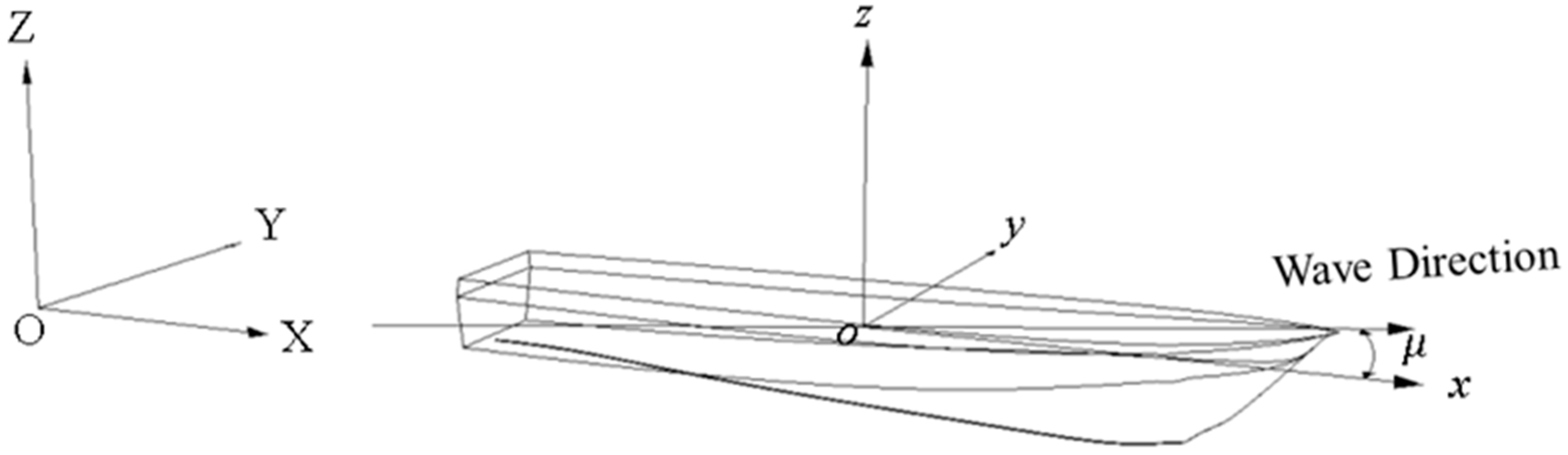
This study used two sets of coordinate systems (Figure 1), the O–XYZ or earth-fixed coordinate system and the o–xyz or body-fixed coordinate system. In frequency-domain motion equations, O–XYZ is a coordinate system fixed in space, whereas o–xyz is fixed to the vessel that passes through the waterline surface of the cross-section of the center of gravity and moves with the hull. Concerning the directions of the different axes, those toward the bow are positive on the OX and ox axes, those toward the port side (from a bird’s-eye view) are positive on the OY and oy axes, and those toward the top of the hull (from a side view) are positive on the OZ and oz axes. Additionally, the hull of the vessel was assumed to be moving forward along the OX axis (positive motion) at a speed of U.
2.2. Basic Assumptions and Boundary Conditions
This study assumed that the vessel sailed at a constant velocity U in deep water with regular waves and that the fluids in the surrounding flow field were ideal non-viscous, incompressible, and non-rotating. Surface tension was not considered, and the hull was assumed to have reached a steady state after experiencing a small-amplitude incident wave. If the incident wave was a, incident wave angle was μ, and incident wave frequency was ω_0, then the incident wave height h was expressed as follows:
where encounter frequency can be expressed as follows:
The incident velocity potential and number of wave cycles are expressed as follows:
where a is the amplitude of the incident wave and g is gravitational acceleration.
According to the Haskind linear theory [5], if the incident wave amplitude and motion response created by such a wave are weak, then the unsteady-state synthesized velocity potential Φ(x,y,z) can be expressed as follows:
where is the incident velocity potential, is the diffraction velocity potential, is the radiation potential created by the motion of various degrees of freedom, is the motion displacement of each degree of freedom, and = 1, 2, 3, 4, 5, and 6 are the surging, swaying, heaving, rolling, pitching, and yawing motion, respectively. Surging, swaying, and heaving motion are the translation amount along the axes, respectively, whereas rolling, pitching, and yawing motion are the rotation amount along the axes, respectively.
The synthesized velocity potential Φ must meet the boundary conditions including the Laplace’s equation, linear free surface conditions, radiation conditions, deep water bottom conditions, and kinematical boundary conditions on the hull surface. Therefore, when a hull is in harmonic motion and moves at a constant speed U along still water, its added mass and damping coefficient can be expressed as follows:
where i, j = 1, 2, …, 6.
2.3. Hydrodynamic Estimation
This study calculated hydrodynamic force using the Kelvin–Havelock singularity method and treated a Green function using the Hess and Smith algorithm. Since Green functions derived from free surface boundary conditions are too complicated to solve, this study assumed reasonably high encounter frequency and low hull speeds to simplify the free surface conditions, and a pulsating Green function was used to obtain the solutions [34,35]. Thus, this Green function can be described as follows:
By considering the pulsating Green function, this study obtained the velocity potential Φ, which was subsequently substituted into Bernoulli’s equation to obtain the hull surface pressure:
This study took the surface integral function along the hull to obtain the wave-exciting force, which is presented as follows:
2.4. Motion Equations
The wave-exciting force, added mass, and damping coefficients were substituted into the motion equations as follows:
where is the mass matrix of the hull, is the added mass matrix, is the restoring matrix, is the displacement corresponding to each degree of freedom, and is the wave-exciting force.
Because the vessel is assumed to be a slender body, the surging motion was minimal and could be excluded from the calculations. Additionally, because the hull shape was symmetrical along the centerline, the horizontal and vertical motion planes did not have coupled motion relationships. The coupled motion relationships of the hull body were only observed for the coupled equations of vertical motion (i.e., heaving and pitching) and those of horizontal motion (i.e., swaying, rolling, and yawing). The coupled equations are listed as follows:
where is the hull mass, is the moment of inertia along the X axis, is the moment of inertia along the Y axis, and is the moment of inertia along the Z axis.
2.5. Wave Spectrum and Significant Ship Motion Values
This study used the three-dimensional energy wave spectrum of short-crested waves introduced by the International Towing Tank Conference (ITTC) and combined it with various RAOs to simulate 6 DOF motion responses of ships under different sea states, and to calculate the significant ship motion values. The ITTC energy wave spectrum comprised two major control factors: significant wave height () and average period (). Formulas for the energy wave spectrum are as follows:
where is the significant wave height, is the average period, is the wave heading angle of the jth wave component with a range of , is the significant ship motion displacement value, is the significant ship motion speed value, is the significant ship motion acceleration value, is the RAO of each motion (i.e., swaying, heaving, rolling, pitching, and yawing), a is the wave amplitude, and is the energy wave spectrum.
3. Data Analysis
Prior to conducting numerical simulation, this study used the specifications of the series 62 craft for reference. Next, 3D computer-aided design (CAD) was performed using the commercial software Rhinoceros 3D, and the ship hull was cut into equally spaced strips. This study then set the draft as well as hull posture, and determined the strip nodes as well as coordinates. The node coordinates, hydrostatic performance, and speed of each hull strip underwater were made into input files, and sea states with significant wave heights () and the average period () were calculated. Subsequently, a ship motion simulation program was installed and calculations were performed. After completing the calculations, the results were presented in graphic form to illustrate the RAOs of the hull motion responses. Additionally, the speed polar diagrams of the semi-planing craft with five degrees of freedom under specific sea states were displayed, revealing the seakeeping performance of the craft.
3.1. Ship Specifications
3.2. Full-Scale Experiments
This study performed full-scale experiments of the series 62 craft at 7, 14, and 33 knots and measured the heaving, rolling, and pitching motion every 30 degrees at wave heading angles ranging from 0 (head sea) to 180 degrees (following sea). The measured data were compared with the simulation data. Since the significant wave height () ranged from 1.2 to 1.4 m, the average cycle () ranged from 4.2 to 4.3 s, and the sea state ranged from 2 to 3 during the three experiments, a significant wave height, average period, and sea state of 1.3 m, 4.2 s, and 3 were selected. The results generated were compared with the simulation data in terms of the heaving, rolling, and pitching motion responses for each wave angle.
The full-scale sea trials were measured at Zuoying harbor for four days in 2003. Each sea trial for an individual heading angle under a specific sailing speed was three minutes. The statistical approach used for significant motion, which is the average value of the highest one-third of all measured results, was based on the zero-up crossing method. The statistical convergence of measured data was achieved using Rayleigh distribution within a 95% confidence interval.
Comparisons for the three different motion responses are detailed as follows:
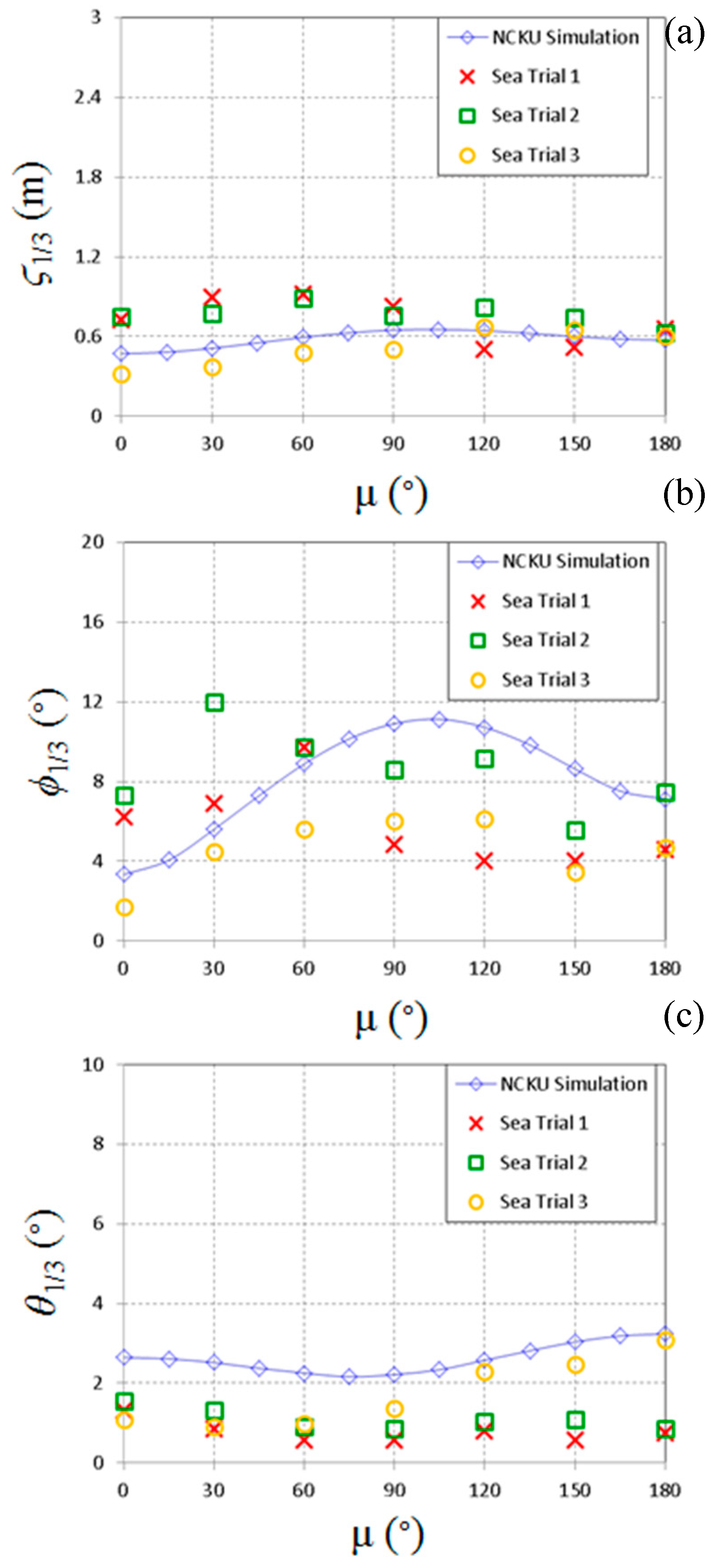
3.2.1. Low Sailing Speed (U = 7 knots, = 1.3 m, and = 4.2 s):
Figure 3a shows a comparison of results from the simulation and the on-board measurement (in terms of heaving motion) for all wave heading angles at a low sailing speed, where the simulation results were sufficiently consistent with the experimental results. In terms of the rolling motion (Figure 3b), the simulation results were consistent with the experimental results, except for wave heading angles of 90°–150°, for which the rolling motion was overestimated. Regarding pitching motion (Figure 3c), the simulation results were sufficiently consistent with the experimental results, except for the wave heading angles of 0°–90°, for which the pitching motion was overestimated.
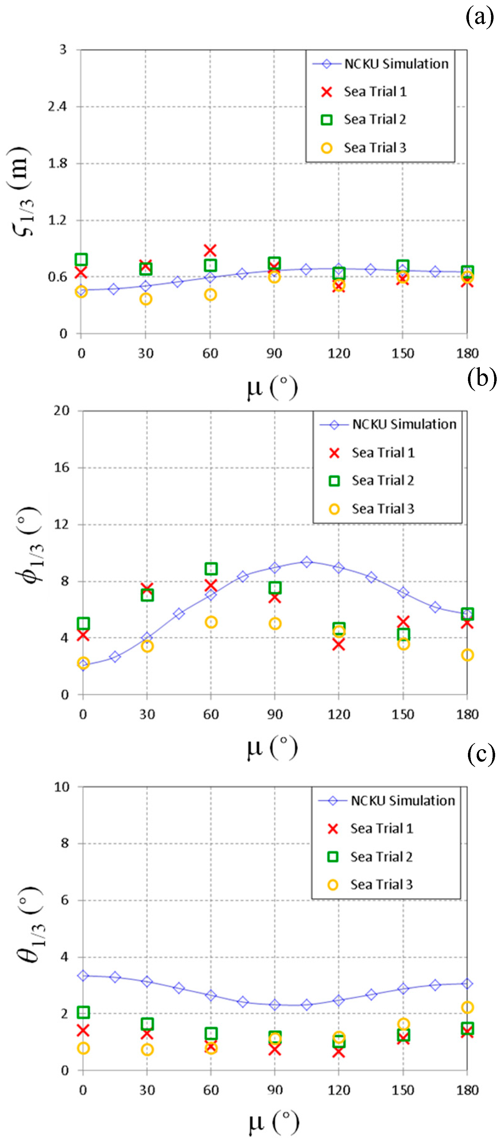
3.2.2. Medium Sailing Speed (U = 14 Knots, H1/3 = 1.3 m, = 4.2 s):
Figure 4a presents a comparison of results from the simulation and on-board measurement (in terms of heaving motion) for all wave heading angles at medium sailing speed, for which the simulation results were sufficiently consistent with the experimental results. In terms of rolling motion (Figure 4b), the simulation results were consistent with the experimental results, except for the wave angles of 90°–150°, for which the rolling motion was overestimated. Regarding pitching motion (Figure 4c), the simulation results were all slight overestimations compared with the experimental results.
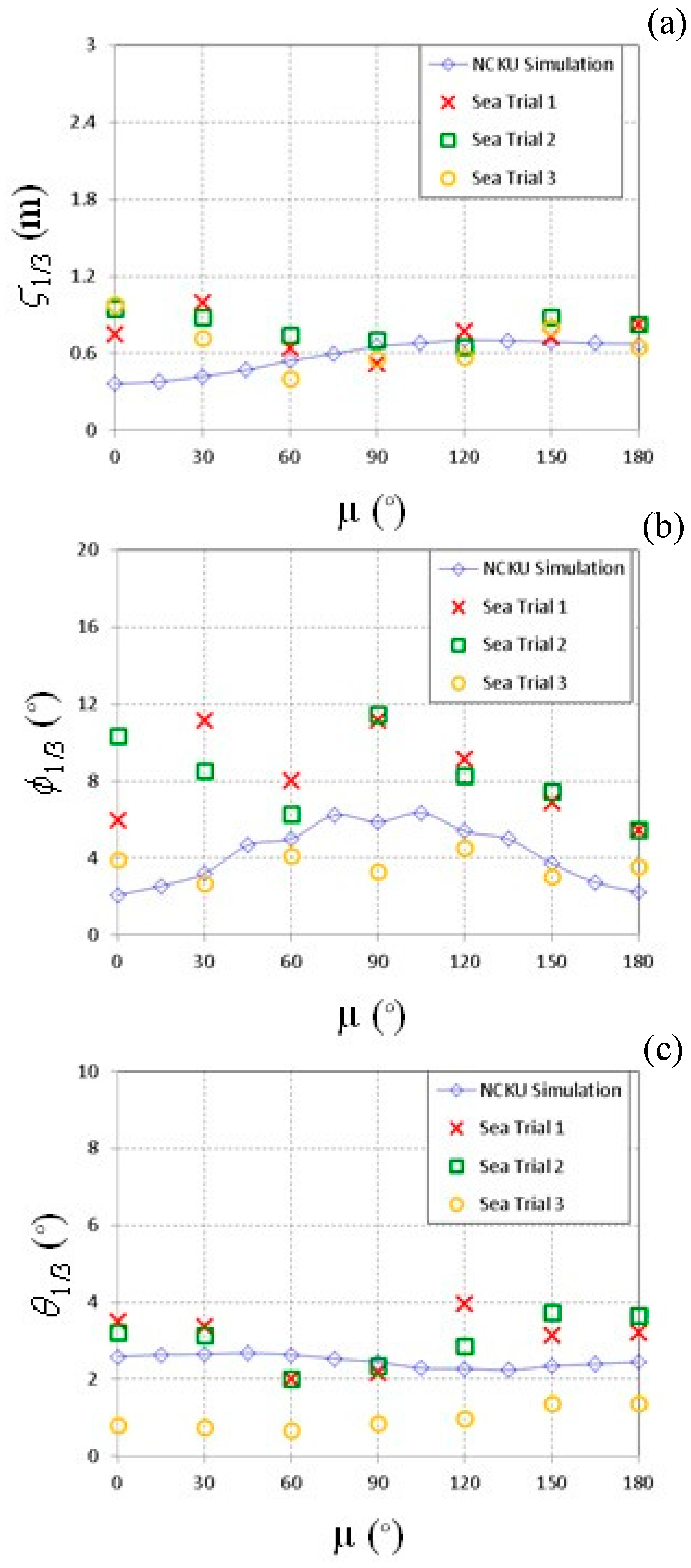
3.2.3. High Sailing Speed (U = 33 Knots, H1/3 = 1.3 m, = 4.2 s):
Figure 5a presents the comparison of results for the simulation and on-board measurement (in terms of heaving motion) for all wave angles at high sailing speed. The simulation results were sufficiently consistent with the experimental results, except for wave angles of 0°–60°, and the heaving motion was underestimated. In terms of rolling motion (Figure 5b), the simulation results were consistent with the experimental results, except for the wave angles of 0°–30° for which the rolling motion was underestimated. Regarding pitching motion (Figure 5c), the simulation results were sufficiently consistent with the experimental results.
Table 2 presents a comparison between the simulation results and the on-board measurements for heaving, rolling, and pitching motion at different sailing speeds in sea state 3. The results indicated that at low and medium sailing speeds, the estimated motion values at some wave heading angles were slight overestimations compared with the experimental results; moreover, at a high sailing speed, the estimated heaving and rolling motions were slightly underestimated compared with the experimental results. The differences between the sea trials and simulation data were mainly caused by southwesterly surges (long waves) in the local summer season. Although there existed some discrepancies due to prediction limitation in the low-frequency region, it was demonstrated that the simulation results agreed reasonably with the on-board measurements.
4. Results and Discussion
4.1. Sailing Speed Comparisons
To explore the effects of various sailing speeds on the swaying, heaving, rolling, pitching, and yawing motion, this study investigated the trim angle of 0° (even keel), 1° by the stern, and 2° by the stern for wave heading angles (i.e., 0°, 90°, and 180°) and compared the results with those obtained using the Froude numbers (Fr = 0.32, 0.65, 0.98, 1.31, 1.64, and 1.97). For a planing or semi-planing craft, dynamic pressure distribution on the high-speed hull during forward motion supported most of the weight and, thus, lifted a large portion of the hull out of the water. According to the definition of Marshall [36], the semi-planing mode was within the range of 0.5 < Fr < 0.85. Therefore, there was only one case of the semi-planing mode, Fr = 0.65, in this study. Both semi-planing and planing modes in this study were assumed to generate an amount of dynamic pressure with their weight supported by buoyancy. As a result of our theory’s limitation, an asymptotic method was proposed to solve the problem of motions of semi-planing crafts in different modes. Since the lines of the hulls were symmetric based on the their centerlines, no swaying, rolling, or yawing motion was used for wave heading angles of 0° and 180°, and only a wave angle of 90° was used to investigate the relationship with sailing speed.
4.1.1. Swaying Motion
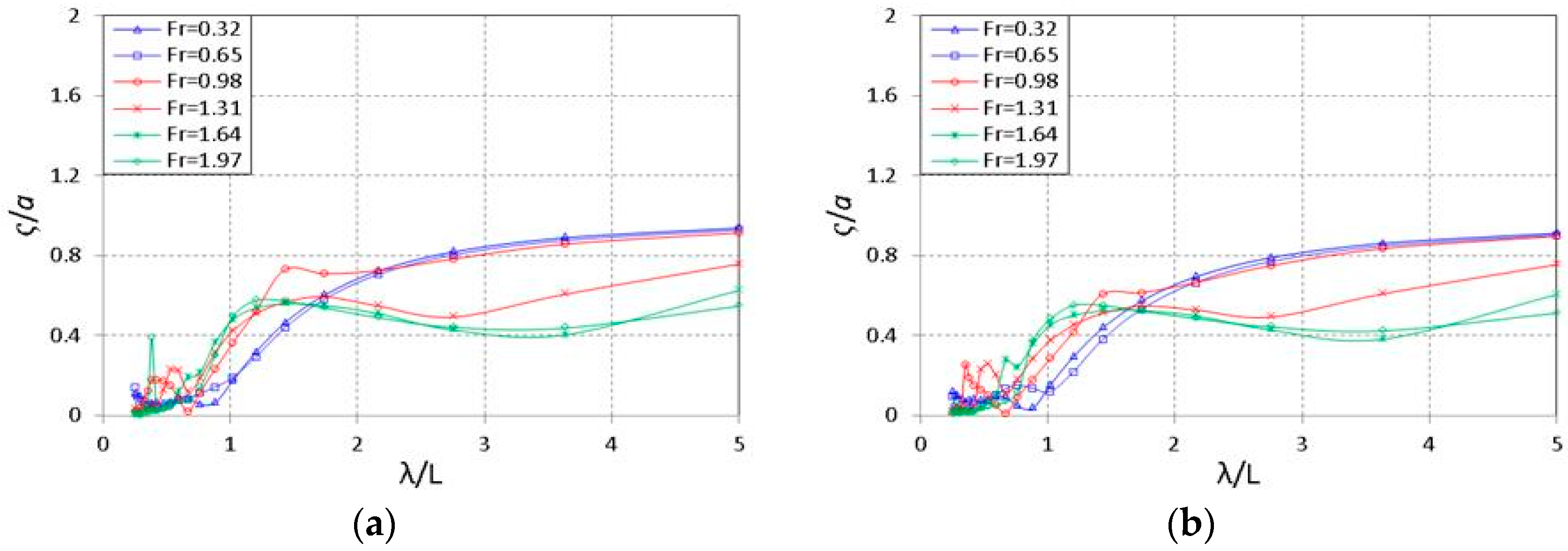
Figure 6a–c indicates that at the trim angles of 0°, 1° by the stern, and 2° by the stern, stronger swaying motion was produced at beam waves as the Froude number increased; moreover, the swaying motion gradually subsided when a relative wave length of λ/L was greater than 1. The swaying motion increased for larger sailing speeds (i.e., the Froude number increased). For medium and large Froude numbers and a wave heading angle of 90°, rolling motion increased when the trim angle increased, suggesting that, for beam waves at medium and high sailing speeds, the swaying motion increased for larger trim angles.
4.1.2. Heaving Motion
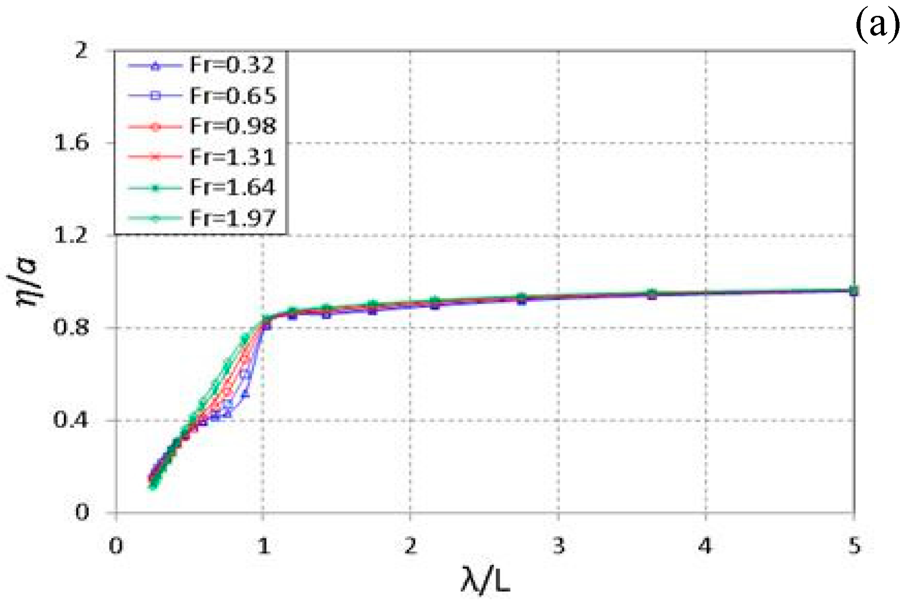
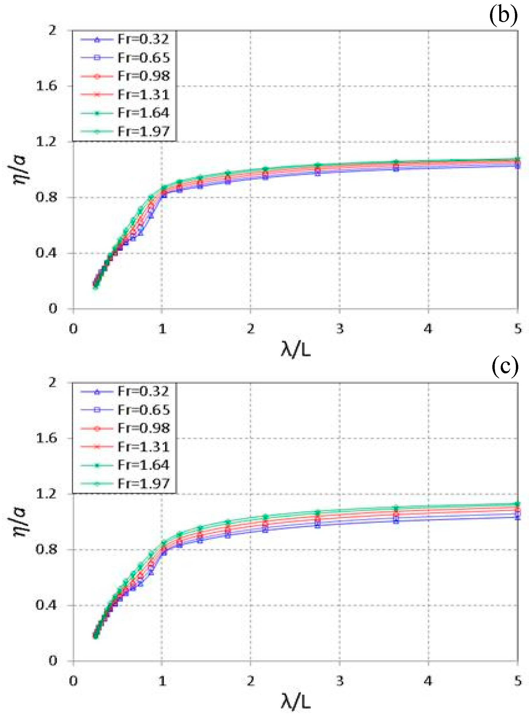
Figure 7a–i reveals that for wave heading angles of 0° and 90°, changing the sailing speed exhibited a minimal effect on the heaving motion. By contrast, at a wave heading angle of 180° and a relative wave length of λ/L ≃ 2 or λ/L > 2, increasing the Froude number increased the heaving motion for all trim angles (0°, 1° by the stern, and 2° by the stern). This signified that when encountering head sea, the larger heaving motion was accompanied by increased sailing speed. For wave heading angles of 0°, 90°, and 180°, and all Froude numbers, changes in trim angle had a minimal effect on heaving motion, demonstrating the weak effect of trim angle on heaving motion.
4.1.3. Rolling Motion
Figure 8a–c demonstrates that for a wave heading angle of 90° and relative wave length of λ/L = 1, a low sailing speed increased the rolling motion for all trim angles. This suggested that, in beam waves, rolling motion decreased as sailing speed increased. For a wave heading angle of 90° and all Froude numbers, the decrease in the trim angle was accompanied with a small rolling motion. This indicated that in beam waves an increase in the trim angle decreased the rolling motion for all sailing speeds.
4.1.4. Pitching Motion
Figure 9a–i displays the pitching motion for various trim angles corresponding to given wave heading angles. For a wave heading angle of 0°, changing the sailing speed exhibited a minimal effect on pitching motion. By contrast, at a wave heading angle of 90° and a relative wave length of ≃ 1 or > 1, an increase in the Froude number decreased the pitching motion. At a wave heading angle of 180° for ≃ 2, an increase in the Froude number was accompanied by an increase in pitching motion for all trim angles. This indicated that when encountering head sea, pitching motion rose when the sailing speed increased and that the ship was in the resonance frequency region.
For the wave heading angles of 0°, 90°, and 180°, and all Froude numbers, changes in trim angle only had a marginal effect on pitching motion, illustrating the small effect of trim angle on pitching motion.
4.1.5. Yawing Motion
Figure 10a–c shows the yawing motion for a wave heading angle of 90° at τ = 0°, 1°and 2°, respectively. The results revealed that for all trim angles, an increase in the Froude number decreased the yawing motion, indicating that in beam waves yawing motion decreased as sailing speed increased. For a wave heading angle of 90° and all Froude numbers, the variation of trim angle had an effect on the yawing motion. This signified that in beam waves increased the trim angle, which increased yawing motion for all sailing speeds.
4.2. Sea State Comparisons
Subsequently, this study examined swaying, heaving, rolling, pitching, and yawing motion under various sea states. The analyzed results indicated that changes in the initial trim angle had little effect on seakeeping performance. Therefore, an even keel was the selected angle for displaying each DOF motion response.
The resulting motion responses were compared for different sea states (1–5), where the Froude numbers used were 0–19.2 (equivalent to 0–36 knots). The significant wave height () and average period () for the various sea states are presented in Table 3. Subsequently, the speed polar diagrams of various motion responses were compared, and the swaying, heaving, rolling, pitching, and yawing motion under the five sea states were obtained for all trim angles.
4.2.1. Swaying Motion
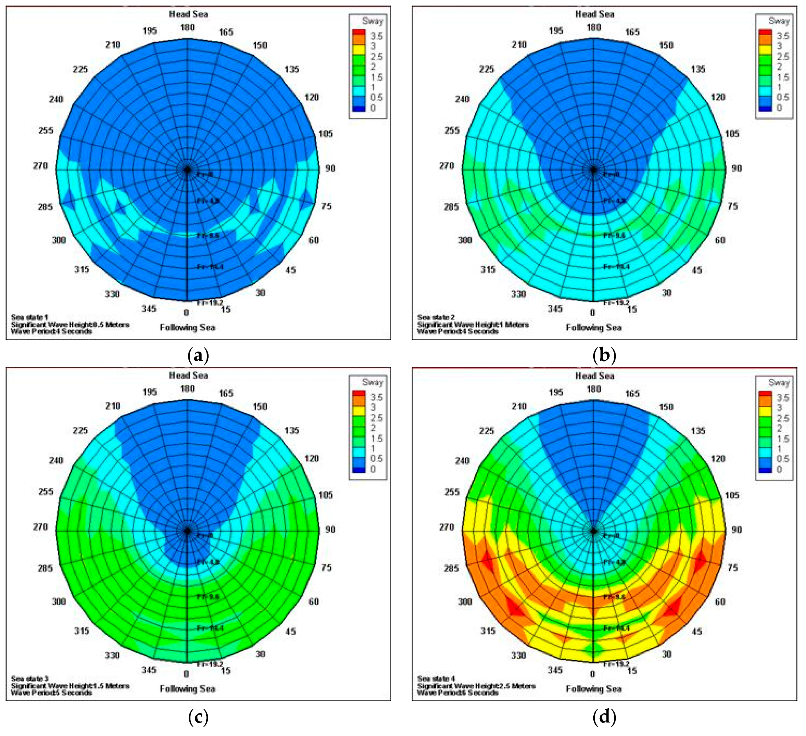
Figure 11a–e displays the speed polar diagrams of the swaying motion by combining sailing speeds with wave heading angles under different sea states (1–5). The results demonstrated that when the sea state worsened, the swaying motion increased substantially for wave heading angles between 30° and 90°; moreover, the strongest swaying motion was observed between the wave heading angles of 45° and 90°. This suggested that for all sailing speeds, when the wave heading angles ranged from quartering to beam waves, the swaying motion increased as the sea state worsened.
4.2.2. Heaving Motion
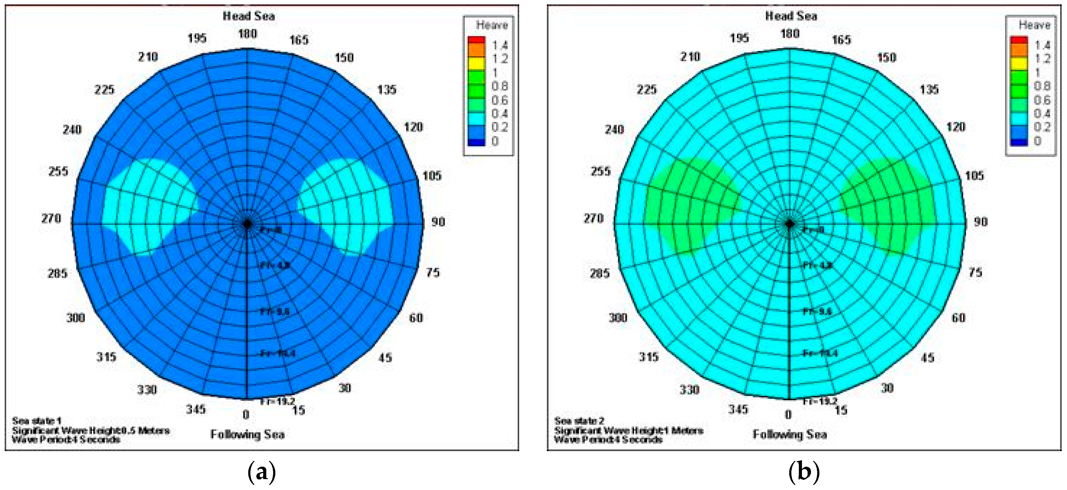
Figure 12a–e displays the speed polar diagrams of the heaving motion by combining sailing speeds with wave heading angles under different sea states (1–5). The results revealed that when the sea state worsened, the heaving motion grew substantially for wave heading angles between 90° and 180°. This signified that for all sailing speeds, when wave heading angles ranged from beam to head seas, heaving motion increased as the sea state worsened.
The figures indicate that when the Froude number was small the heaving motion was strongest at a wave heading angle of 90°. When the Froude number was large or in the middle range, the strongest heaving motion was produced at the wave heading angles of 135° and 180°. These results suggested that at low sailing speeds, heaving motion was strongly affected by beam waves and that at medium and high sailing speeds, heaving motion was strongly affected by bow and head seas.
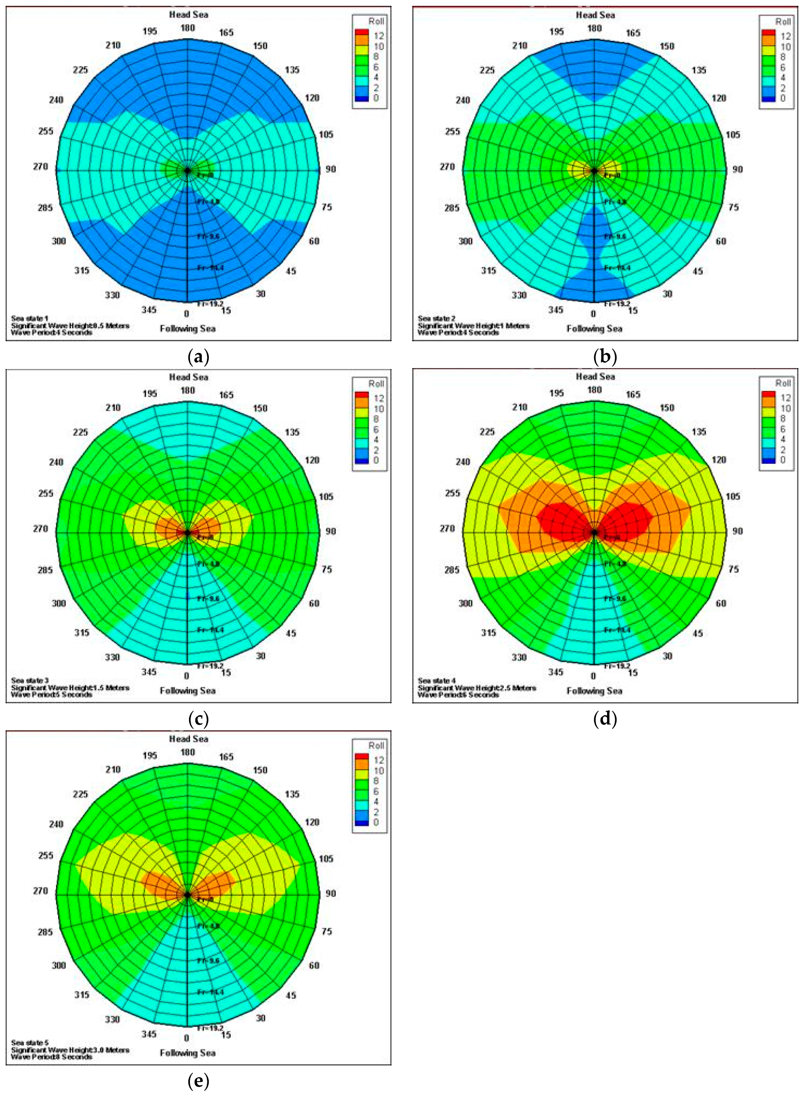
4.2.3. Rolling Motion
Figure 13a–e displays the speed polar diagrams of rolling motion in combination with sailing speeds and wave heading angles under different sea states (1–5). The results suggest that when the sea state worsened, rolling motion increased noticeably for wave heading angles between 45° and 135°, and that the strongest rolling motion was observed for wave heading angles between 90° and 135°. This indicated that for all sailing speeds, when wave heading angles ranged from beam to bow seas, rolling motion increased as the sea state worsened.
For all Froude numbers, a discernible resonance of rolling motion was generated at the wave angles of 90° and 135°. Additionally, at a wave heading angle of 135°, increasing the Froude number caused the significant resonance of rolling motion. This signified that for all sailing speeds, rolling motion was strongly affected by beam and bow seas.
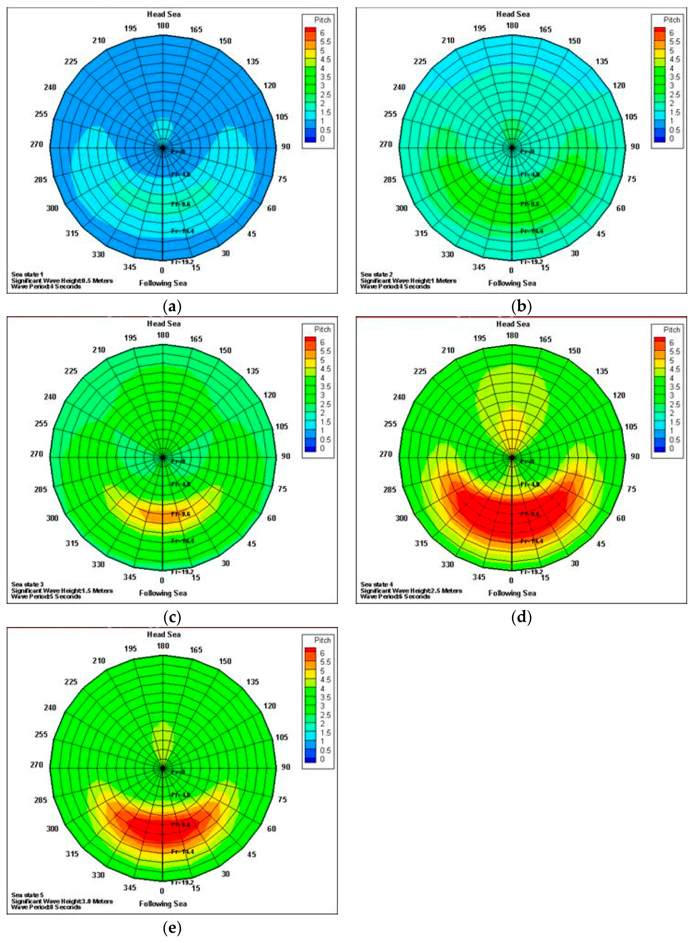
4.2.4. Pitching Motion
Figure 14a–e displays the speed polar diagrams of pitching motion for different wave heading angles and sailing speeds under sea states (1–5). The diagrams indicate that when the sea state worsened, the value of pitching motion enhanced substantially for wave heading angles between 0° and 90°, and that the strongest pitching motion was observed for wave heading angles between 0° and 45°. This suggests that pitching motion increased as the sea state worsened, when the craft moved at moderate speeds in following or quartering seas.
The figure demonstrates that when the Froude number was small, the pitching motion was relatively strong at a wave heading angle of 180°. When the Froude number was in the middle range, pitching motion was relatively strong at a wave heading angle of 0°. When the Froude number was large, pitching motion was relatively strong at a wave angle of 180°. These results indicated that at low and high sailing speeds, pitching motion was strongly affected by head sea and that at medium sailing speeds, pitching motion was strongly affected by following sea.
4.2.5. Yawing Motion
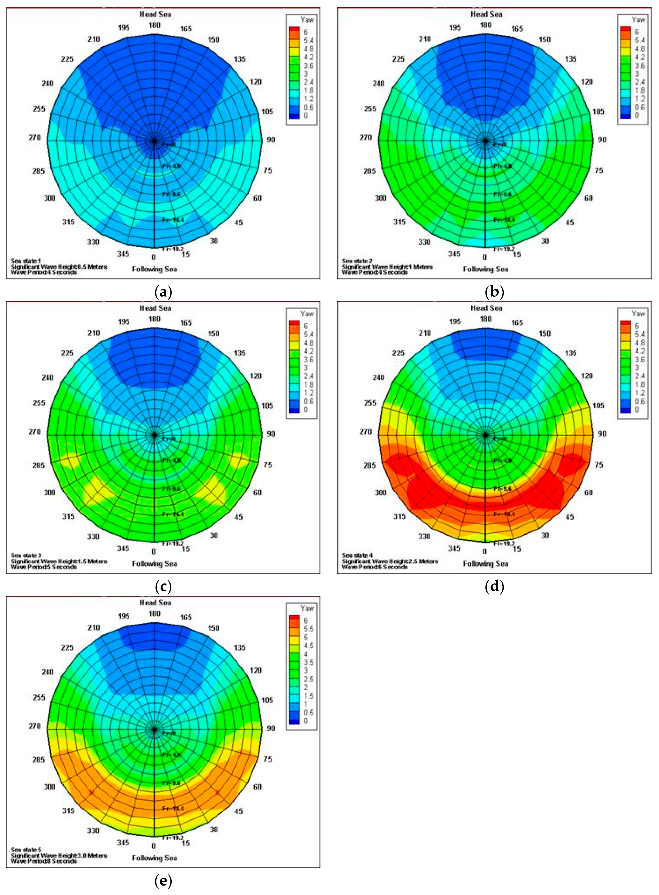
Figure 15a–e displays the speed polar diagrams of yawing motion for different wave heading angles at various sailing speeds under sea states (1–5). The diagrams indicated that when the sea state worsened, yawing motion strengthened considerably for wave angles between 45° and 90°. This suggests that for all sailing speeds, when the wave heading angle ranged from quartering to beam waves, yawing motion increased as the sea state worsened.
For all Froude numbers, the resonance of yawing motion was evidently produced at a wave heading angle of 45°, and the yawing motion increased when the Froude number increased. This indicated that for all sailing speeds, yawing motion was strongly affected by quartering seas.
5. Conclusions
This study established a seakeeping program combining two-dimensional strip theory with the two-dimensional Green function based on the potential theory to solve boundary values and motion responses of a semi-planing craft. The simulation results can be used to help examine the seakeeping performance of high-speed crafts and to create a database for further route planning. By comparing the calculation results with those measured from on-board measurements, the reliability of the calculation results was confirmed. The findings are as follows:
- (1)
- The swaying motion was strongly affected by beam waves at low sailing speeds and by quartering waves and increases in trim angle at medium and high speeds. The swaying motion was strongly affected by increases in sailing speed and worsening of the sea state.
- (2)
- The heaving motion was strongly affected by beam waves at low sailing speeds and by bow and head waves at medium and high speeds. The heaving motion was not affected by the trim angle for any sea state but was strongly affected by increases in sailing speed and worsening of the sea state.
- (3)
- In beam waves, the rolling motion decreased as the sailing speed and trim angle increased. The rolling motion was strongly affected by worsening of the sea state, particularly in beam waves.
- (4)
- The pitching motion was evidently influenced by head seas at low or high sailing speeds, and by worsening of the sea state at medium sailing speed or in following seas. The pitching motion was relatively unaffected by trim angles for all sea states.
- (5)
- In beam waves the yawing motion decreased as the sailing speed increased, and increased when the trim increased. When the wave heading angle ranged from quartering to beam waves, the yawing motion was considerably dominated by worsening of the sea state.
The simulation results were within an acceptable range, verifying the reliability of the methods introduced in this study for assessing the seakeeping performance of high-speed semi-planing craft in comparison with full-scale on-board measurements. Although the crafts usually have different trim angles at high speeds due to dynamic lift under various loading and draft conditions, this study only investigated the trim angles of 0° (even keel), 1° by the stern, and 2° by the stern. No predictions could be made for the trim angles at any sailing speed during the transition or planing modes. Thus, when analyzing the seakeeping performance of high-speed crafts in the future, the trim angles under various sailing speeds, loading and draft conditions should be considered to enable the prediction of seakeeping performance and improve the accuracy of simulations. Such information can provide designers with preliminary seakeeping performance information for high-speed crafts.
Author Contributions
Y.-H.L. is the principal researcher of this study, and C.-W.L. conducts the numerical simulation and data analysis.
Funding
This research was funded by Ministry of Science and Technology (Taiwan), grant number MOST 107-2218-E-006-052 and MOST 107-2221-E-006-229.
Acknowledgments
The authors would like to express their thanks to the Ministry of Science and Technology for a grant under Contract No. MOST 107-2218-E-006-052. The authors also thank Ming-Chun Fang for his advice on this study.
Conflicts of Interest
The authors declare no conflict of interest.
References
- Yousefi, R.; Shafaghat, R.; Shakeri, M. Hydrodynamic analysis techniques for high-speed planing hulls. Appl. Ocean Res. 2013, 42, 105–113. [Google Scholar] [CrossRef]
- Korvin-Kroukovsky, B. Investigation of ship motions in regular waves. Trans. SNAME 1955, 63, 386–435. [Google Scholar]
- Jacobs, W.R. The analytical calculation of ship bending moments in regular waves. J. Ship Res. 1958, 2, 20–29. [Google Scholar]
- Salvesen, N.; Tuck, E.; Faltinsen, O. Ship motions and sea loads. Trans. SNAME 1970, 78, 250–287. [Google Scholar]
- Kim, C.H.; Chou, F.S.; Tien, D. Motions and Hydrodynamic Loads of a Ship Advancing in Oblique Waves; Society of Naval Architects and Marine Engineers: Jersey City, NJ, USA, 1980; pp. 225–256. [Google Scholar]
- Fang, M.-C. Time simulation of water shipping for a ship advancing in large longitudinal waves. J. Ship Res. 1993, 37, 126–137. [Google Scholar]
- Fang, M.; Chen, G.; Lee, Z. The Bank Effect on the Motion Behaviors of a Ship Advancing in Waves. J. Taiwan Soc. Nav. Archit. Mar. Eng. 2013, 32, 47–54. [Google Scholar]
- Haskind, M. The hydrodynamic theory of ship oscillations in rolling and pitching. Prikl. Mat. Mekh. 1946, 10, 33–66. [Google Scholar]
- Haskind, M. The oscillation of a ship in still water. Izv. Akad. Nauk SSSR Otd. Tekh. Nauk 1946, 1, 23–34. [Google Scholar]
- Chang, M.-S. Computations of three-dimensional ship motions with forward speed. In Proceedings of the 2nd International Conference on Numerical Ship Hydrodynamics, Berkeley, CA, USA, 19–21 September 1977; pp. 124–135. [Google Scholar]
- Inglis, R. Calculation of velocity potential of a translating, pulsating source. Trans. RINA 1980, 123, 163–175. [Google Scholar]
- Guevel, P.; Bougis, J. Ship-motions with forward speed in infinite depth. Int. Shipbuild. Prog. 1982, 29, 103–117. [Google Scholar] [CrossRef]
- King, B.; Beck, R.; Magee, A. Seakeeping calculations with forward speed using time domain analysis. In Proceedings of the 17th Symposium on Naval Hydrodynamics, The Hague, The Netherlands, 28 August–2 September 1988. [Google Scholar]
- Lin, W.-M.; Yue, D. Numerical solutions for large-amplitude ship motions in the time domain. In Proceedings of the 18th Symposium on Naval Hydrodynamics, Ann Arbor, MI, USA, 19–24 August 1990. [Google Scholar]
- Alexander, B.; Josh, H. Motions and Loads of a Trimaran Traveling in Regular Waves; FAST: London, UK, 2001. [Google Scholar]
- Bingham, H.; Korsmeyer, F.; Newman, J.N.; Osborne, G.E. The simulation of ship motions. In Proceedings of the Sixth International Conference on Numerical Ship Hydrodynamics; National Academies Press: Washington, DC, USA, 1994; pp. 561–580. [Google Scholar]
- Martin, M. Theoretical Prediction of Motions of High-Speed Planing Boats in Waves; David W. Taylor Naval Ship Research and Development Center: Bethesda, MD, USA, 1976. [Google Scholar]
- Zarnick, E.E. A Nonlinear Mathematical Model of Motions of a Planing Boat in Regular Waves; David W. Taylor Naval Ship Research and Development Center: Bethesda, MD, USA, 1978. [Google Scholar]
- Keuning, J.A.; Gerritsma, J.; van Terwisga, P. Resistance Tests of a Series Planing Hull Forms with 30 Degrees Deadrise Angle, and a Calculation Model Based on This and Similar Systematic Series; Delft University of Technology: Delft, The Netherlands, 1993. [Google Scholar]
- Akers, R.H. Dynamic analysis of planing hulls in the vertical plane. In Proceedings of the Society of Naval Architects and Marine Engineers, New England Section, Jersey City, NJ, USA, 1999. [Google Scholar]
- Keuning, J.; Toxopeus, S.; Pinkster, J. The effect of bow shape on the seakeeping performance of a fast monohull. In Proceedings of the FAST Conference, Southampton, UK, 4–6 September 2001. [Google Scholar]
- Sariöz, K.; Sariöz, E. Practical seakeeping performance measures for high speed displacement vessels. Nav. Eng. J. 2006, 118, 23–36. [Google Scholar] [CrossRef]
- Van Deyzen, A. A nonlinear mathematical model of motions of a planning monohull in head seas. In Proceedings of the 6th International Conference on High Performance Marine Vehicles (HIPER’08), Naples, Italy, 18–19 September 2008. [Google Scholar]
- De Jong, P. Seakeeping Behaviour of High Speed Ships: An Experimental and Numerical Study. Ph.D. Thesis, Delft University of Technology, Delft, The Netherlands, 2011. [Google Scholar]
- Mousaviraad, S.M.; Wang, Z.; Stern, F. URANS studies of hydrodynamic performance and slamming loads on high-speed planing hulls in calm water and waves for deep and shallow conditions. Appl. Ocean. Res. 2015, 51, 222–240. [Google Scholar] [CrossRef] [Green Version]
- De Luca, F.; Mancini, S.; Miranda, S.; Pensa, C. An extended verification and validation study of CFD simulations for planing hulls. J. Ship Res. 2016, 60, 101–118. [Google Scholar] [CrossRef]
- Blount, D.L.; Clement, E.P. Resistance tests of a systematic series of planing hull forms. SNAME Trans. 1963, 71, 491–579. [Google Scholar]
- Hassan, G.; Su, Y.-M. Determining the hydrodynamic forces on a planing hull in steady motion. J. Mar. Sci. Appl. 2008, 7, 147–156. [Google Scholar] [CrossRef]
- Liu, C.; Wang, C. Interference effect of catamaran planing hulls. J. Hydronaut. 1979, 13, 31–32. [Google Scholar] [CrossRef]
- Lamb, H. Hydrodynamics; Cambridge University Press: Cambridge, UK, 1932. [Google Scholar]
- Maruo, H. Two dimensional theory of the hydroplane. In Proceedings of the 1st Japan National Congress on Applied Mechanics, Science Council of Japan, Tokyo, Japan, 1952; pp. 409–415. [Google Scholar]
- Cumberbatch, E. Two-dimensional planing at high Froude number. J. Fluid Mech. 1958, 4, 466–478. [Google Scholar] [CrossRef]
- Frandoli, P.; Merola, L.; Pino, E.; Sebastiani, L. The role of seakeeping calculations at the preliminary design stage. In Proceedings of the NAV 2000 Conference, Venice, Italy, 19–22 September 2000; pp. 951–959. [Google Scholar]
- Fang, M.-C.; Chen, G.-R. On the nonlinear hydrodynamic forces for a ship advancing in waves. Ocean Eng. 2006, 33, 2119–2134. [Google Scholar] [CrossRef]
- Fang, M.-C.; Chen, G.-R. The relative motion and wave elevation between two floating structures in waves. In Proceedings of the Eleventh International Offshore and Polar Engineering Conference Stavanger, Stavanger, Norway, 17–22 June 2001; pp. 361–368. [Google Scholar]
- Marshall, R. All about Powerboats: Understanding Design and Performance; McGraw Hill Professional: New York, NY, USA, 2002. [Google Scholar]
Figure 1.
Schematic of the hull coordinate systems.

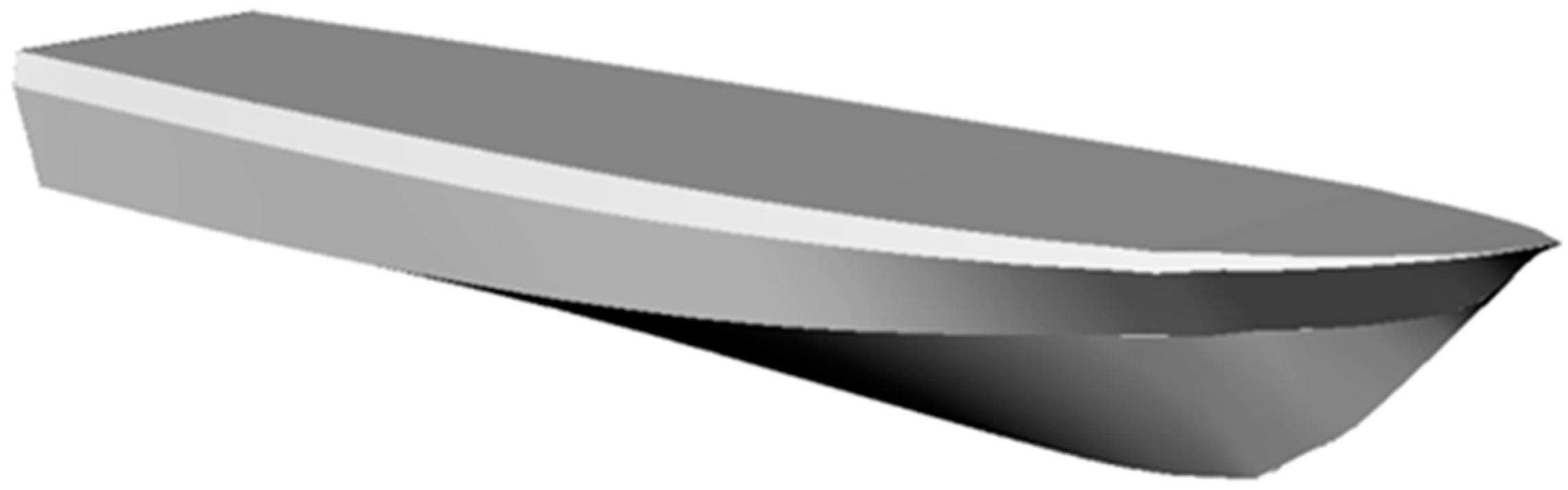
Figure 2.
Complete schematic diagram of the series 62 craft.

Figure 3.
Comparison of results for the simulation and on-board measurement in terms of (a) heaving, (b) rolling, and (c) pitching motion at low sailing speed.
Figure 3.
Comparison of results for the simulation and on-board measurement in terms of (a) heaving, (b) rolling, and (c) pitching motion at low sailing speed.

Figure 4.
Comparison of results for the simulation and the on-board measurement in terms of (a) heaving, (b) rolling, and (c) pitching motion at medium sailing speed.
Figure 4.
Comparison of results for the simulation and the on-board measurement in terms of (a) heaving, (b) rolling, and (c) pitching motion at medium sailing speed.

Figure 5.
Comparison of results for the simulation and on-board measurement in terms of (a) heaving, (b) rolling, and (c) pitching motion at high sailing speed.
Figure 5.
Comparison of results for the simulation and on-board measurement in terms of (a) heaving, (b) rolling, and (c) pitching motion at high sailing speed.

Figure 6.
RAO comparison of swaying motion for various Froude numbers at μ = 90° corresponding to trim angles of (a) τ = 0°, (b) τ = 1°, and (c) τ = 2°, respectively.
Figure 6.
RAO comparison of swaying motion for various Froude numbers at μ = 90° corresponding to trim angles of (a) τ = 0°, (b) τ = 1°, and (c) τ = 2°, respectively.


Figure 7.
RAO comparison of the heaving motion for various Froude numbers and the trim angles of (a) τ = 0°, (b) τ = 1°, or (c) τ = 2° when μ = 0°; (d) τ = 0°, (e) τ = 1°, and (f) τ = 2° when μ = 90°; and (g) τ = 0°, (h) τ = 1°, and (i) τ = 2° when μ = 180°.
Figure 7.
RAO comparison of the heaving motion for various Froude numbers and the trim angles of (a) τ = 0°, (b) τ = 1°, or (c) τ = 2° when μ = 0°; (d) τ = 0°, (e) τ = 1°, and (f) τ = 2° when μ = 90°; and (g) τ = 0°, (h) τ = 1°, and (i) τ = 2° when μ = 180°.


Figure 8.
RAO comparison of rolling motion for various Froude numbers at μ = 90° corresponding to trim angles of (a) τ = 0°, (b) τ = 1°, and (c) τ = 2°, respectively.
Figure 8.
RAO comparison of rolling motion for various Froude numbers at μ = 90° corresponding to trim angles of (a) τ = 0°, (b) τ = 1°, and (c) τ = 2°, respectively.

Figure 9.
RAO comparison of pitching motion for various Froude numbers and trim angles of (a) τ = 0°, (b) τ = 1°, or (c) τ = 2° when μ = 0°; (d) τ = 0°, (e) τ = 1°, and (f) τ = 2° when μ = 90°; and (g) τ = 0°, (h) τ = 1°, and (i) τ = 2° when μ = 180°.
Figure 9.
RAO comparison of pitching motion for various Froude numbers and trim angles of (a) τ = 0°, (b) τ = 1°, or (c) τ = 2° when μ = 0°; (d) τ = 0°, (e) τ = 1°, and (f) τ = 2° when μ = 90°; and (g) τ = 0°, (h) τ = 1°, and (i) τ = 2° when μ = 180°.

Figure 10.
RAO comparison of yawing motion for various Froude numbers at μ = 90° with respect to (a) τ = 0°, (b) τ = 1°, and (c) τ = 2°.
Figure 10.
RAO comparison of yawing motion for various Froude numbers at μ = 90° with respect to (a) τ = 0°, (b) τ = 1°, and (c) τ = 2°.

Figure 11.
Speed polar diagrams of swaying motion in combination with sailing speeds and wave heading angles under sea states of (a) 1, (b) 2, (c) 3, (d) 4, and (e) 5, respectively.
Figure 11.
Speed polar diagrams of swaying motion in combination with sailing speeds and wave heading angles under sea states of (a) 1, (b) 2, (c) 3, (d) 4, and (e) 5, respectively.


Figure 12.
Speed polar diagrams of heaving motion in combination with sailing speeds and wave heading angles under sea states of (a) 1, (b) 2, (c) 3, (d) 4, and (e) 5, respectively.
Figure 12.
Speed polar diagrams of heaving motion in combination with sailing speeds and wave heading angles under sea states of (a) 1, (b) 2, (c) 3, (d) 4, and (e) 5, respectively.


Figure 13.
Speed polar diagrams of rolling motion in combination with sailing speeds and wave heading angles under sea states of (a) 1, (b) 2, (c) 3, (d) 4, and (e) 5, respectively.
Figure 13.
Speed polar diagrams of rolling motion in combination with sailing speeds and wave heading angles under sea states of (a) 1, (b) 2, (c) 3, (d) 4, and (e) 5, respectively.

Figure 14.
Speed polar diagrams of pitching motion at various sailing speeds for different wave heading angles under sea state (a) 1, (b) 2, (c) 3, (d) 4, and (e) 5, respectively.
Figure 14.
Speed polar diagrams of pitching motion at various sailing speeds for different wave heading angles under sea state (a) 1, (b) 2, (c) 3, (d) 4, and (e) 5, respectively.

Figure 15.
Speed polar diagrams of yawing motion at various sailing speeds for different heading angles when sea state was (a) 1, (b) 2, (c) 3, (d) 4, and (e) 5, respectively.
Figure 15.
Speed polar diagrams of yawing motion at various sailing speeds for different heading angles when sea state was (a) 1, (b) 2, (c) 3, (d) 4, and (e) 5, respectively.


Table 1.
Specifications of the series 62 craft.
| Hull Dimensions | Size |
|---|---|
| Hull length (L) (m) | 34 |
| Hull width (B) (m) | 7.6 |
| Draft (T) (m) | 1.7 |
| Displacement volume ∇ () | 171 |
| Block coefficient () | 0.461 |
| Prismatic coefficient () | 0.685 |
| Transverse metacentric height () (m) | 1.723 |
| Longitudinal metacentric height () (m) | 59.3 |
| Longitudinal center of gravity (LCG) (m) | 13.1 |
Table 2.
Mean deviations of the simulation data (in terms of heaving, rolling, and pitching motion) for all wave heading angles.
Table 2.
Mean deviations of the simulation data (in terms of heaving, rolling, and pitching motion) for all wave heading angles.
| Knots | Motion | 0°~60° | 60°~120° | 120°~180° |
|---|---|---|---|---|
| 7 | Heave (m) | −0.15 | −0.07 | −0.03 |
| Roll (°) | −0.78 | 3.1 | 3.37 | |
| Pitch (°) | 1.43 | 1.32 | 1.53 | |
| 14 | Heave (m) | −0.11 | 0.02 | 0.08 |
| Roll (°) | −1.31 | 2.34 | 2.93 | |
| Pitch (°) | 1.82 | 1.49 | 1.48 | |
| 33 | Heave (m) | −0.34 | 0.02 | −0.05 |
| Roll (°) | −3.37 | −1.95 | −2.21 | |
| Pitch (°) | 0.46 | 0.46 | −0.34 |
Table 3.
Significant wave height and average period for the five sea states.
| Sea State | 1 | 2 | 3 | 4 | 5 |
|---|---|---|---|---|---|
| Significant wave height ( | 0.5 | 0.8 | 1.6 | 2.4 | 3.2 |
| Average period () | 4 | 4 | 5 | 6 | 8 |
© 2019 by the authors. Licensee MDPI, Basel, Switzerland. This article is an open access article distributed under the terms and conditions of the Creative Commons Attribution (CC BY) license (http://creativecommons.org/licenses/by/4.0/).
Share and Cite
MDPI and ACS Style
Lin, Y.-H.; Lin, C.-W. Numerical Simulation of Seakeeping Performance on the Preliminary Design of a Semi-Planing Craft. J. Mar. Sci. Eng. 2019, 7, 199. https://doi.org/10.3390/jmse7070199
AMA Style
Lin Y-H, Lin C-W. Numerical Simulation of Seakeeping Performance on the Preliminary Design of a Semi-Planing Craft. Journal of Marine Science and Engineering. 2019; 7(7):199. https://doi.org/10.3390/jmse7070199
Chicago/Turabian StyleLin, Yu-Hsien, and Chia-Wei Lin. 2019. "Numerical Simulation of Seakeeping Performance on the Preliminary Design of a Semi-Planing Craft" Journal of Marine Science and Engineering 7, no. 7: 199. https://doi.org/10.3390/jmse7070199
Note that from the first issue of 2016, this journal uses article numbers instead of page numbers. See further details here.