Shallow Landslide Susceptibility Mapping: A Comparison between Logistic Model Tree, Logistic Regression, Naïve Bayes Tree, Artificial Neural Network, and Support Vector Machine Algorithms

Abstract

Shallow landslides damage buildings and other infrastructure, disrupt agriculture practices, and can cause social upheaval and loss of life. As a result, many scientists study the phenomenon, and some of them have focused on producing landslide susceptibility maps that can be used by land-use managers to reduce injury and damage. This paper contributes to this effort by comparing the power and effectiveness of five machine learning, benchmark algorithms—Logistic Model Tree, Logistic Regression, Naïve Bayes Tree, Artificial Neural Network, and Support Vector Machine—in creating a reliable shallow landslide susceptibility map for Bijar City in Kurdistan province, Iran. Twenty conditioning factors were applied to 111 shallow landslides and tested using the One-R attribute evaluation (ORAE) technique for modeling and validation processes. The performance of the models was assessed by statistical-based indexes including sensitivity, specificity, accuracy, mean absolute error (MAE), root mean square error (RMSE), and area under the receiver operatic characteristic curve (AUC). Results indicate that all the five machine learning models performed well for shallow landslide susceptibility assessment, but the Logistic Model Tree model (AUC = 0.932) had the highest goodness-of-fit and prediction accuracy, followed by the Logistic Regression (AUC = 0.932), Naïve Bayes Tree (AUC = 0.864), ANN (AUC = 0.860), and Support Vector Machine (AUC = 0.834) models. Therefore, we recommend the use of the Logistic Model Tree model in shallow landslide mapping programs in semi-arid regions to help decision makers, planners, land-use managers, and government agencies mitigate the hazard and risk.

1. Introduction

Landslides are a serious hazard in many parts of the world. According to a report by the World Bank, approximately 300 million people around the world live in landslide-prone areas [1,2] and economic losses from landslides amount to about USD 20 billion, with the largest losses incurred by the United States, Italy, Japan, India, China, and Germany [3,4,5].

Although landslides commonly can be attributed to natural (topographic, geological, geophysical, and hydrological) factors, Iran, like other countries, has experienced a large number of human-induced landslides in recent years due to ground modification and construction that has been driven by economic and population growth [5,6,7]. The country lies within a seismically active mountainous region, and large earthquakes trigger landslides in mountainous parts of the country, notably the Alborz and Zagros Mountains [8,9]. Nearly 2600 landslides were reported in Iran up to 2000 [10], and those in the 20th century alone are responsible for 30,000 deaths and nearly 60,000 injuries [11].

One strategy for reducing loss of life and damage from landslides is to prepare maps that identify areas vulnerable to landslides [12,13]. Landslide susceptibility may be defined as the likelihood that a landslide will occur in a given area or at a specific site [14]. Maps that show the propensity of an area to slope failure are termed “landslide susceptibility maps” [15,16]. These maps help land-use managers and other government officials to proactively reduce future losses from landslides [17].

In recent years, a variety of qualitative knowledge-driven and quantitative data-driven statistical and artificial intelligence (AI) techniques have been developed and used to predict landslides [18]. Although each method has its advantages and disadvantages, the Logistic Regression (LR) model method has been the first choice of most researchers [19]. The advantage of Logistic Regression is that variables can be discrete or any combination of types, and do not have to be normally distributed [20]. The LR uses a maximum likelihood estimation function to estimate the probability of an event occurring [21]. Developing accurate and robust models from environmental data has been a challenge for environmental scientists because of the “curse of multidimensionality,” i.e., environmental data are diverse in nature and come from a variety of sources, such as field surveys, air photo and satellite images, and historical records [17,18,22].

This problem has been addressed through the development and application of machine learning algorithms, which are able to handle large volumes of non-linear and complex data derived from different sources and reported at a variety of scales. These algorithms have been extensively used in natural hazard studies, for example: flooding [23,24,25,26,27,28,29,30,31,32,33], wildfire [34,35], dust storm [36], sinkhole formation [37], drought [38,39], earthquakes [40,41], gully erosion [42,43,44], land/ground subsidence [45,46], groundwater contamination [26,47,48,49,50,51], and landslides [17,52,53,54,55,56,57,58,59,60,61,62,63,64,65,66,67,68,69,70,71,72,73,74,75,76,77,78]. They can extract informative patterns in historical data to predict future events [79].

A wide variety of machine learning algorithms have been developed to overcome data challenges and develop accurate and robust landslide susceptibility prediction models. These algorithms extract related information patterns in historical data to forecast future events. Techniques that have been applied to develop landslide susceptibility maps include weight-of-evidence (WoE) [80], Logistic Regression (LR) [81,82,83], Bayesian Logistic Regression (BLR) [30,72], Artificial Neural Networks (ANN) [58,63,84,85,86], Evidential Belief Functions (EBF) [57,87], Fuzzy Logic Algorithm [88,89], Support Vector Machines (SVM) [52,90,91], Naïve Bayes Tree (NBT) [17,74,92,93], Alternating Decision Tree (ADTree) [45,54,69], Logistic Model Tree (LMT) [30,45,79], Kernel Logistic Regression (KLR) [94], Adaptive Neuro Fuzzy Inference System (ANFIS) [95], Gaussian process regression (GPR) [96], and Bagging Functional Tree (BFT) [97].

In particular, ensemble and hybrid machine learning techniques have provided promising results and have been widely used around the world in recent years [17,18,22,52,56,98,99]. Their base classifiers have good predictive ability and have been successful in predicting landslide-prone areas. For example, Naïve Bayes Tree (NBT), Logistic Model Tree (LMT), LR, Support Vector Machine (SVM), and Artificial Neural Network (ANN), the algorithms used in this study, have successfully identified landslide-susceptible areas in up to 90% of all cases [100,101,102].

The prediction accuracy of landslide susceptibility models depends on the geographical region, landslide conditioning factors (LCF), sample size, and on hyper parameter tuning [18,99]. As yet, there is no consensus as to which models are most appropriate for specific regions, hence it is necessary to use a variety of methods in each study area to determine the method with the highest predictive power. The main objective of this study is to spatially predict shallow landslides around Bijar city in eastern Kurdistan Province, Iran, using soft computing benchmark models, specifically LMT, LR, NBT, ANN, and SVM. The LR, ANN, and SVM algorithms are considered among some landslide researchers to be superior to other machine learning and conventional methods [22,103,104]. LMT is a decision tree algorithm that combines a decision tree and a Logistic Regression function in leaves. It has been used in many fields of environmental and natural hazard research, such as landslides, floods, gully erosion, sinkhole formation, land subsidence, and groundwater potential mapping [22,45,87,105,106]. In this study, we identify and rank the most important factors responsible for shallow landslides in the Bijar study area. We evaluate the reliability and predictive power of the five machine learning models based on sensitivity, specificity, accuracy, kappa, root mean square error (RMSE), area under the ROC curve (AUC), and Wilcoxon and Friedman statistical tests. Data processing was done using ArcGIS 10.3 (ESRI, Redlands, CA, USA), and the machine learning algorithms were modeled with WEKA 3.9 software (University of Waikato, Waikato, New Zealand).

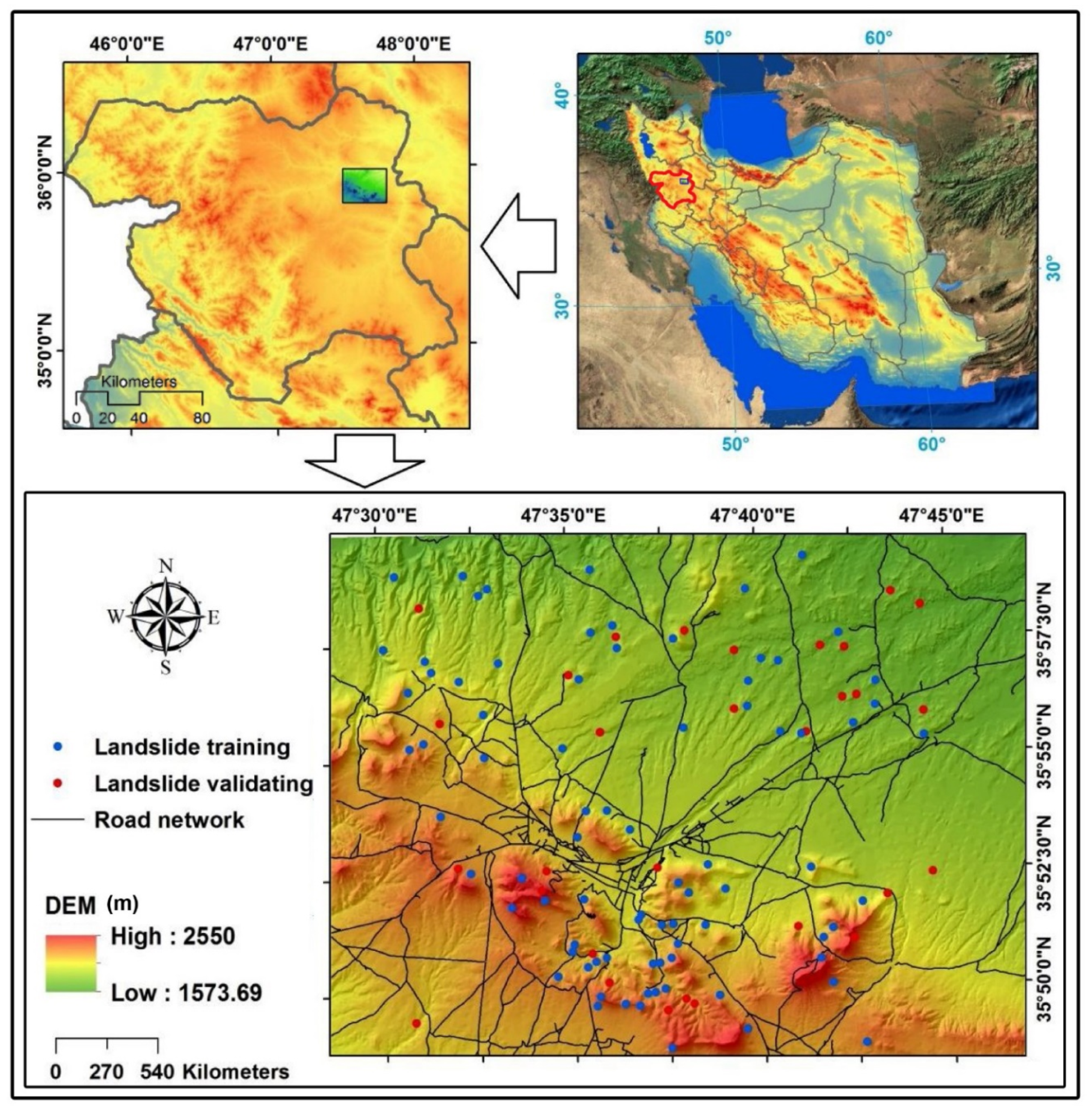
2. Description of the Study Area

The study area (598 km²; 35°48′25″ N to 35°09′50″ N and 47°28′50″ E to 47°46′44″ E) is located around Bijar City in the eastern part of the Kurdistan Province in Iran (Figure 1). The regional climate is cool, with annual average temperatures ranging from 4.4 °C to 13.4 °C. Mean annual rainfall recorded between 1987 and 2010 at Bijar City was about 338 mm. Although annual precipitation is low, short-duration storms can produce large amounts of rain. Intensities of about 34 mm/h have a return period of about 20 years. The area is hilly, with elevations ranging from 250 to 1573 m asl (above sea level) and slopes up to 60°. There are four types of land cover in the Bijar region: (1) barren lands (0.07%), (2) cultivated lands (53.62%), (3) residential areas (1.26%), and (4) grasslands (45.05%). Geologically, 94% of the area is underlain by conglomerate, siltstone, shale, and marl, and 6% is underlain by volcanic rocks [17,65,69].

3. Data Preparation

3.1. Landslide Inventory Map

An accurate landslide inventory map is one of the prerequisite tools for achieving a successful landslide modeling prediction and must be prepared with care [107]. Some more important information can be derived from this inventory map, such as locations of occurred landslides, landslides type, frequencies of landslides, causes and triggers of landslides (i.e., earthquakes, intense rainfall, and rapid snowmelt) [65]. In this study, we obtained 111 landslide polygons from the Forests, Rangeland and Watershed Management Organization of Iran and checked them by examining aerial photographs (1:40,000 scale) and satellite images, and by inspection in the field. Field surveys showed that most of the landslides have resulted from human modification of slopes [84]. Most are shallow landslides (depths less than 3 m) and include slumps (70.60%), complex landslides (22.4%), and falls (6.3%) [86]. Minimum and maximum lengths of landslide are, respectively, 70 m and 280 m; the mean and median values are 37 m and 26 m. Landslide widths range from 7 to 293 m; mean and median values are 37 m and 63 m [65,69].

3.2. Landslide Conditioning Factors

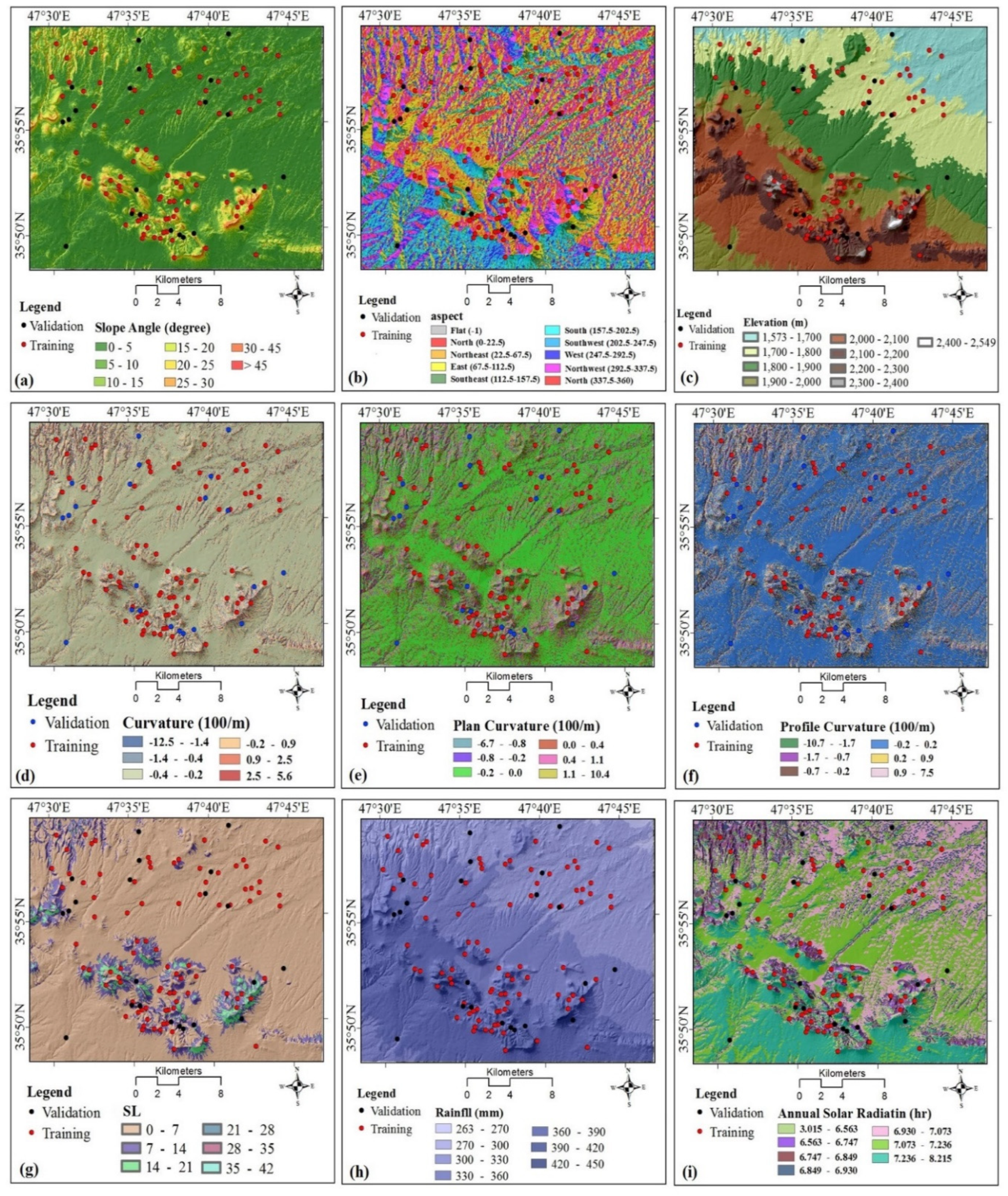
In this study, we selected 20 landslide conditioning factors (LCF) based on the literature and data availability and partitioned them into five categories: topography (slope angle, slope aspect, elevation, curvature, profile curvature, plan curvature, and sediment transport index); hydrology (rainfall, solar radiation, sediment transport power (SPI), topographic wetness index (TWI), distance to rivers, and river density); geology (lithology, distance to fault, and fault density); land cover (land use and normalized difference vegetation index (NDVI)); and human-related factors (distance to road and road density). A digital elevation model (DEM) with a raster resolution of 28.5 m × 28.5 m was constructed from ASTER GDEM-1 satellite images taken in August 2005. The DEM was resampled to a raster resolution of 10 m to prepare data layers using the “Resample tool” in Arc GIS 10.3. The 20 LCM are briefly described below.

3.2.1. Slope Angle

Slope is an expression of changes in elevations over distance and is expressed in this study in degrees. All other things being equal, steeper slopes are more susceptible to landslides, thus slope is an important conditioning factor in landslide susceptibility prediction modeling [5,17,18,108,109]. This conditioning factor was divided into eight classes using the manual classification method: (1) 0°–5°, (2) 5°–10°, (3)10°–15°, (4) 15°–20°, (5) 20°–25°, (6) 25°–30°, (7) 30°–45°, and (8) >45° (Figure 2a).

3.2.2. Slope Aspect

Slope aspect is a measure of the cardinal direction of a slope, expressed relative to north (00) [110]. It has been shown to be related to the evapotranspiration in hilly areas and thus to be an important LCF [111,112]. In the present study, slope aspect was divided into nine classes: (1) flat, (2) north, (3) northeast, (4) east, (5) southeast, (6) south, (7) southwest, (8) west, and (9) northwest (Figure 2b).

3.2.3. Elevation

The incidence and frequency of landslides may differ with elevation and thus can be an important LCD. Both temperature and precipitation affect soil moisture and commonly change with elevation. Lower elevations also may be preferentially used for roads, the construction of which might trigger landslides in hilly or mountainous areas [113]. Elevation may not have a fixed pattern, and it likely has different impacts on landslides depending on geology and the geographical region being studied [114]. Elevation was divided into nine classes using the manual classification method: (1) 1573–1700, (2) 1700–1800, (3) 1800–1900, (4) 1900–2000, (5) 2000–2100, (6) 2100–2200, (7) 2200–2300, (8) 2300–2400, and (9) >2400 m (Figure 2c).

3.2.4. Curvature

The curvature of a slope can be concave, convex, or zero [109]. This LCM was divided into six classes using the natural break classification method: (1) [(−12.5)–(−1.4)]; (2) [(−1.4)–(−0.4)]; (3) [(−0.4)–(−0.2)]; (4) [(−0.2)–0.9]; (5) [0.9–2.5]; and (6) [2.5–15.6] (Figure 2d).

3.2.5. Plan Curvature

Plan curvature is a measure of the concavity or convexity of a slope. It is used to analyze gradients between ridges and valleys. In this study, cells with concave curvature have positive values and cells with convex curvature have negative values. Slope erosion and water infiltration may relate to plan curvature; consequently, it is commonly used in developing landslide susceptibility prediction models [115,116]. We divided plan curvature into six classes using the natural break classification method: (1) [(−6.7)–(−0.8)]; (2) [(−0.8)–(−0.2)]; (3) [(−0.2)–0]; (4) [0–0.4]; (5) [0.4–1.1]; and (6) [1.1–10.4] (Figure 2e).

3.2.6. Profile Curvature

Profile curvature is a measure of the concavity or convexity of the maximum slope, typically along stream channels. It can be positive, zero, or negative, depending on whether the surface is, respectively, upwardly concave, linear, or convex. As profile curvature influences water flow over the slope, it is considered to be one of the most important LCF in landslide susceptibility prediction models. We divided profile curvature into six classes using the natural break classification method: (1) [(−10.7)–(−1.7)], (2) [(−1.7)–(−0.7)], (3) [(−0.7)–(−0.2)], (4) [(−0.2)–0.2], (5) [0.2–0.9], and (6) [0.9–7.5] (Figure 2f).

3.2.7. Slope Length

Slope length (SL) is the distance between the origin of overland flow and the point where runoff enters a defined channel [117]. It provides a measure of the erosive capability of overland flow [118]. We divided slope length into six classes using the natural break classification method: (1) 0–7; (2) 7–14; (3) 14–21; (4) 21–28; (5) 28–35; and (6) 35–42 (Figure 2g).

3.2.8. Rainfall

The amount and intensity of rainfall is commonly positively correlated with landslide frequency, but the relationship depends strongly on topography. Rainfall on well drained, relatively flat terrain may have less impact on slope stability than it does in hilly areas [114]. We constructed a rainfall map based on mean annual rainfall over the period 1980–2016 based on records from nine rain gauge stations inside and outside the study area. Rainfall was divided into seven classes using the natural break classification method: (1) 263–270; (2) 270–300; (3) 300–330; (4) 330–360; (5) 360–390; (6) 390–420; and (7) 420–450 mm (Figure 2h).

3.2.9. Annual Solar Radiation

Solar radiation directly affects evapotranspiration and is also influenced by topography. It may have an indirect impact on landslide susceptibility [113]. A layer for this conditioning factor was prepared using the “annual solar radiation” tool in ArcGIS 10.2, and then divided into seven classes using the natural break classification method: (1) 3.015–6.563, (2) 5.563–6.747, (3) 6.747–6.849, (4) 6.849–6.930, (5) 6.930–7.073, (6) 7.073–7.236, and (7) 7.236–8.215 h (Figure 2i).

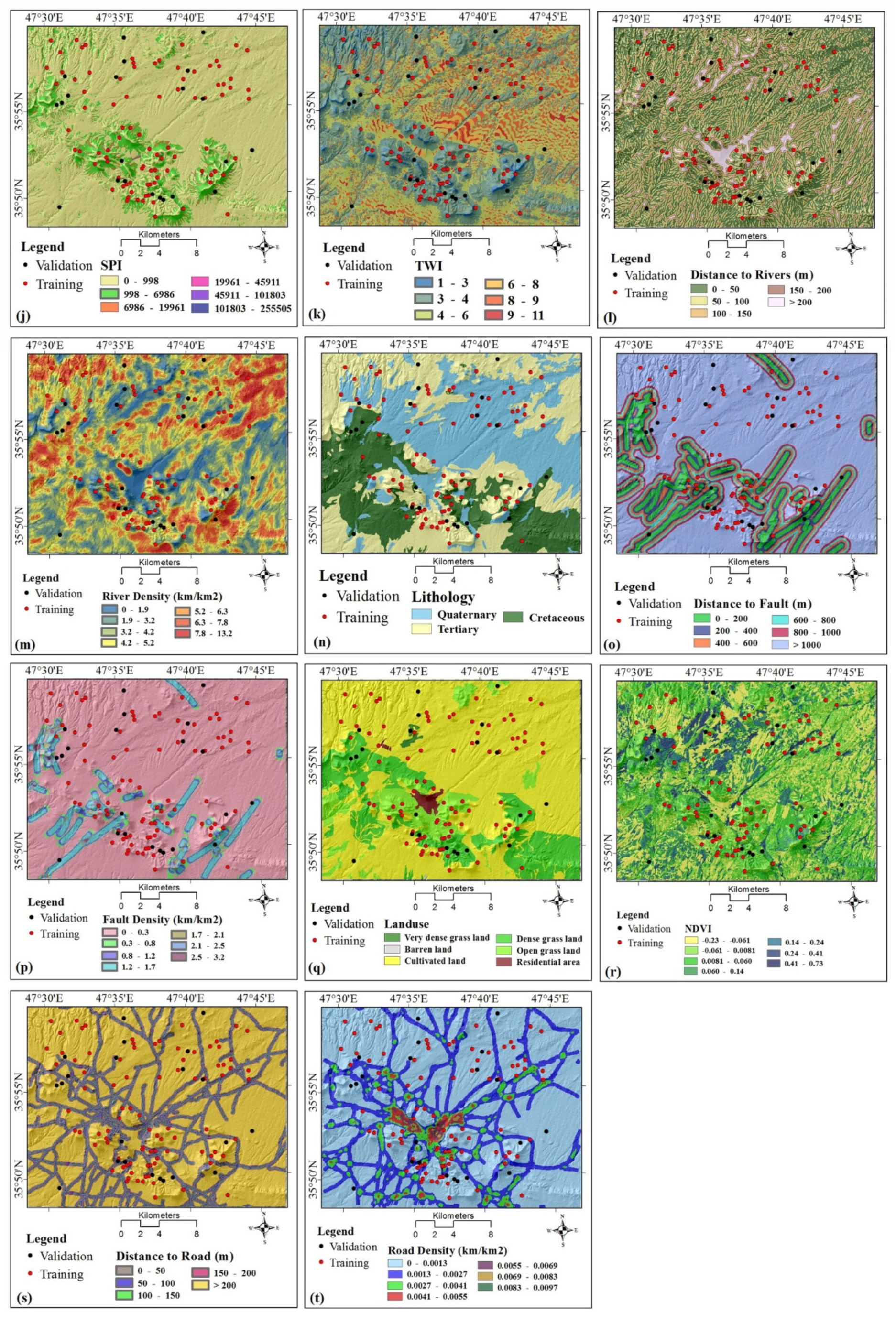
3.2.10. Stream Power Index

Stream power index (SPI) is a measure of the erosive capacity of flowing water and is a product of the slope gradient and catchment area [119], and is a good candidate for landslide susceptibility prediction model development. We derived SPI from the DEM in the SAGA software environment and then divided it into six groups: (1) 0–998; (2) 998–6986; (3) 6986–19,961; (4) 19,961–45,911; (5) 45,911–101,803; and (6) 101,803–255,505 (Figure 2j).

3.2.11. Topographic Wetness Index

Topographic wetness index (TWI) is a measure of water accumulation degree at a site [118]. As TWI increases, landslide susceptibility may also increase. We calculated TWI from the DEM using SAGA software and then divided it into six groups using the natural break classification method: (1) 1–3; (2) 3–4; (3) 4–6; (4) 6–8; (5) 8–9; and (6) 9–11 (Figure 2k).

3.2.12. Distance to Rivers

A river might undercut a side slope, increasing the likelihood of a landslide. We infer, however, that this is only likely to happen if the river borders a slope steeper than 15°. Thus, when constructing the distance-to-river map, we did not consider instances where rivers border slopes of less than 15°. We constructed the distance-to-river map with buffers around rivers using the Euclidean distance tool in ArcGIS 10.5, and then divided distances into five groups using the natural break classification method: (1) 0–50, (2) 50–100, (3) 100–150, (4) 150–200, and (5) >200 m (Figure 2l).

3.2.13. River Density

Rivers density is positively related to the frequency of landslides in mountainous regions [120], in part through its effects on groundwater recharge. The river density layer was prepared using the line density tool in ArcGIS 10.2 and then divided into seven groups using the natural break classification methods: (1) 0–1.9, (2) 1.9–3.2, (3) 3.2–4.2, (4) 4.2–5.2, (5) 5.2–6.3, (6) 6.3–7.8, and (7) 7.8–13.2 km/km² (Figure 2m).

3.2.14. Lithology

Lithology affects soil porosity and permeability [121] and also rock strength. The lithology map of the study area was generated from a 1:100,000-scale geological map produced by the Geological Survey of Iran and verified through field work and air photo interpretation. We grouped geological units into three groups: Quaternary, Tertiary, and Cretaceous (Figure 2n).

3.2.15. Distance to Faults

Many landslides are associated with faults due to the lower strength of rocks along these structures. We prepared the distance-to-fault layer from the geological map using Euclidean distance tool in ArcGIS 10.2; values range from 0 to 2000 m. We divided the LCF into five groups using the natural break classification method: (1) 0–200, (2) 200–400, (3) 400–600, (4) 600–800, (5) 800–1000 and (6) >1000 m (Figure 2o).

3.2.16. Fault Density

Fault density provides an aerial measure of highly fractured, and thus weak, rocks [122]. The fault density layer was produced from the geological map using the line density tool in ArcGIS 10.2 and then divided into seven groups using the natural break classification method: (1) 0–0.3, (2) 0.3–0.8, (3) 0.8–1.2, (4) 1.2–1.7, (5) 1.7–2.1, (6) 2.1–2.5, and (7) 2.5–3.2 km/km² (Figure 2p).

3.2.17. Land Use

Land use is a significant factor for slope stability because development and utilization of the land affects infiltration, surface runoff, and vegetation [123]. The land-use layer in the present study was generated from Landsat 7 OLI sensor images. Six land-use types were identified: (1) very dense grassland, (2) barren land, (3) cultivated land, (4) dense grassland, (5) open grassland, and (6) residential area (Figure 2q).

3.2.18. NDVI

The normalized difference vegetation index (NDVI) provides a measure of vegetation greenness and thus biomass. A change in vegetated areas might lead to slope failures [124]. We prepared the NDVI map using Landsat 8 OLI sensor images from Landsat 8 in ENVI5.1. NDVI values were divided into six categories: (1) [(−0.23)–(−0.061)], (2) [(−0.061)–(−0.0081)], (3) [(−0.0081)–(0.060)], (4) [(0.060)–0.14], (5) [0.14–0.24], (6) [0.24–0.41], and (7) [0.41–0.73] (Figure 2r).

3.2.19. Distance to Roads

Road construction can increase the likelihood of landslides in hilly and mountainous areas by reducing the rock and sediment strength, steepening slopes, and creating roadside fills [125]. Only roads that undercut slopes steeper than 15° were included in the distance-to-road map. We added buffer zones to calculate distances from roads at five intervals: (1) 0–50, (2) 50–100, (3) 100–150, (4) 150–200, and (5) >200 m (Figure 2s).

3.2.20. Road Density

Road density is the cumulative length of roads per unit area [126]. Most landslides in the study area are near roads, therefore road density provides a measure of the cumulative impacts of road construction on the occurrence of landslides [17]. The road density layer has seven categories: (1) 0–0.0013, (2) 0.0013–0.0027, (3) 0.0027–0.0041, (4) 0.0041–0.0055, (5) 0.0055–0.0069, (6) 0.0069–0.0083, and (7) 0.0083–0.0097 km/km² (Figure 2t).

4. Methods

4.1. Naïve Bayes Tree

The Naïve Bayes Tree (NBT) model, which was first proposed by Kohavi [127], combines two classifiers: the ID3 decision tree, which is responsible for the classification process and splitting the tree, and Naïve Bayes. It offers several advantages over other machine learning models, specifically the ability to (1) represent knowledge, (2) manage complexity, (3) select candidate concepts, (4) process small datasets, and (5) minimize noise in training datasets [128]. The modeling and classification processes can be performed on even a small amount of data [111].

The first step in NBT modeling is to grow a tree based on the entropy (degree of disorder) feature selection method. If S is a set of the training dataset and $\left|S\right|$ is the total number of conditioning factors, the factors can be grouped into n classes $S_i(i=1,2,\dots ,n)$. ${\left|S\right|}_i$ is the number of conditioning factors belonging to the class $S_i$. The classification of S can be calculated based on the expected entropy as follows:

$$\mathrm{Entropy}(\mathrm{S})=-{\displaystyle \sum _{i=1}^n(\frac{\left|{\mathrm{S}}_{\mathrm{i}}\right|}{\left|\mathrm{S}\right|}})\mathrm{l}\mathrm{o}{\mathrm{g}}_2[(\frac{\left|{\mathrm{S}}_{\mathrm{i}}\right|}{\left|\mathrm{S}\right|})]$$

(1)

Consider attribute A, for example aspect, in set S. The expected entropy can be expressed as:

$${\mathrm{Entropy}}_{\mathrm{A}}(\mathrm{S})=-{\displaystyle \sum _{i=1}^n\frac{\left|{\mathrm{S}}_{\mathrm{i}}\right|}{\left|\mathrm{S}\right|}}\times \mathrm{I}\mathrm{n}\mathrm{f}\mathrm{o}({\mathrm{S}}_{\mathrm{i}})$$

(2)

The difference between $Entropy(S)$ and ${Entropy}_A(S)$ is represented as the information gain (InfoGain):

$$\mathrm{InfoGain}(\mathrm{A})=\mathrm{E}\mathrm{n}\mathrm{t}\mathrm{r}\mathrm{o}\mathrm{p}\mathrm{y}(\mathrm{S})-\mathrm{E}\mathrm{n}\mathrm{t}\mathrm{r}\mathrm{o}\mathrm{p}{\mathrm{y}}_{\mathrm{A}}(\mathrm{S})$$

(3)

The information gain ratio (IGR) is calculated according to the following equation:

$$GainRatio(A)=\frac{\mathrm{InfoGain}(\mathrm{A})}{SplitInfo(A)}=\frac{\mathrm{E}\mathrm{n}\mathrm{t}\mathrm{r}\mathrm{o}\mathrm{p}\mathrm{y}(\mathrm{S})-\mathrm{E}\mathrm{n}\mathrm{t}\mathrm{r}\mathrm{o}\mathrm{p}{\mathrm{y}}_{\mathrm{A}}(\mathrm{S})}{-{\displaystyle \sum _{i=1}^n(\frac{\left|S_j\right|}{\left|S\right|}}){\log }_2[(\frac{\left|S_j\right|}{\left|S\right|})]}$$

(4)

Naïve Bayes is performed on the leaves of the tree after the tree is grown and split. It assumes the conditional independence among attributes $x_1,x_2,\dots ,x_n$. Let $k_i(landslide and non-landslide)$ be an attribute of class set K. The a posteriori probability can be computed as follows:

$$k_{NB}=\arg {\max }_{Z_i}PP(k_i){\displaystyle \prod _{i=1}^n\frac{1}{\sqrt{2\pi \sigma }}}{e}^{\frac{-{(d_i-\sigma )}^2}{2{\sigma }^2}}$$

(5)

where $PP(k_i)$ denotes the a posteriori probability of the output class label $k_i(landslide and non-landslide)$, and σ and ε are, respectively, the mean and standard deviation of $d_i$.

4.2. Logistic Regression

Logistic Regression determines the relation of landslide occurrence and possible causative factors, and has been widely used in landslide susceptibility mapping [129,130]. It can be used when the dependent variable is binary or dichotomous. The dependent variable (Y) is the absence (0) or presence (1) of a landslide. The conditional probability that a landslide occurs is denoted by $P(y=\mathit{1}|x)$. The logit of the LR model is transformed by the following equation:

$$logit\left(y\right)=b_0+b_1{x}_1+b_2{x}_2+\dots +b_n{x}_n$$

(6)

where $b_0$ is the intercept of the equation, and $b_1$, $b_2$, …,$b_n$ are the coefficients of independent variables $x_1$, $x_2$, …,$x_n$. The probability $\mathrm{P}(\mathrm{y}=1|\mathrm{x})$ is computed in the LR model as follows:

$$\mathrm{P}(\mathrm{y}=1|\mathrm{x})=\frac{1}{1+{\mathrm{e}}^{-(}{}^{{\mathrm{b}}_0+{\mathrm{b}}_1{\mathrm{x}}_1+{\mathrm{b}}_2{\mathrm{x}}_2+\dots +{\mathrm{b}}_{\mathrm{n}}{\mathrm{x}}_{\mathrm{n}})}}$$

(7)

where e is the constant 2.718.

4.3. Logistic Model Tree

Logistic Model Tree combines the C4.5 algorithm [131] and Logistic Regression (LR) functions. The IGR technique is applied to split the tree into nodes and leaves, and the LogitBoost algorithm [132] is used to fit the logistics regression functions at a tree node. The C4.5 algorithm uses the entropy technique for feature selection because it is the fastest method for providing reliable classification accuracy [133]. The over-fitting problem, which is an important challenge in LMT modeling, is overcome using the CART algorithm, which prunes the tree for modeling the training dataset [129].

The IGR can be formulated as follows:

$$\mathrm{Gain}\mathrm{ratio}\left(\mathrm{A}\right)=\frac{\mathrm{gain}\left(\mathrm{A}\right)}{\mathrm{split}\mathrm{info}\left(\mathrm{A}\right)}$$

(8)

where $gain(A)$ is the information after attribute A is selected as a test for classification of the training samples and $split info(A)$ is the information generated when x training samples are categorized into n subsets [131].

In the next step, the LogitBoost algorithm performs additive Logistic Regression with least-squares fit for each class Ci (landslide or non-landslide) according to the following equation [134]:

$${\mathrm{L}}_c(x)={\displaystyle \sum _{i=1}^{CF}{\alpha }_i}{x}_i+{\alpha }_0$$

(9)

where $L_c(x)$ is the least-squares fit, and $CF$ ${\alpha }_i$ are, respectively, the number of landslide conditioning factors and the coefficient of the ith element of vector x. The a posteriori probabilities in the leaves of the LMT are calculated using the linear Logistic Regression model [132]:

$$\mathrm{p}(\mathrm{c}|\mathrm{x})=\frac{\exp ({\mathrm{L}}_{\mathrm{c}}(\mathrm{x}))}{{\displaystyle \sum _{{\mathrm{c}}^{\prime }=1}^{\mathrm{c}}\exp ({\mathrm{L}}_{{\mathrm{c}}^{\prime }}(\mathrm{x}))}}$$

(10)

where c is the number of landslide classes and Lc(x), the least-squares fit, is transformed in such a way that ${\displaystyle \sum _{{\mathrm{c}}^{\prime }=1}^{\mathrm{c}}{\mathrm{L}}_c(\mathrm{x})=0}$.

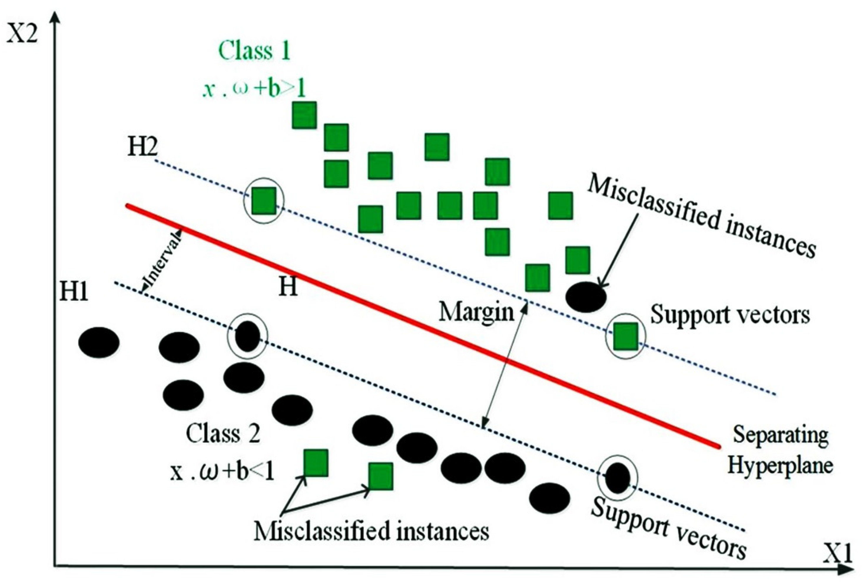
4.4. Support Vector Machine

Support Vector Machine is a set of machine learning techniques based on the concept of an optimal separating hyperplane [135]. SVM finds the widest margin between two classes in feature space. A typical SVM model can be a two-class or multi-class model (combination of a chain of two-class SVMs), as shown in Figure 3. The two-class SVM is the most frequently used machine learning model [94,136,137]. During model performance, the separating hyperplane is one of the probable planes separating the two classes. SVM finds an optimal hyperplane by distinguishing the two classes, using the following equation [135]:

$$\underset{w,b,\xi }{\overset{}{Min}}: \frac{1}{2}{w}^{T}w+c{{\displaystyle {\sum }_{i=1}^1\xi }}_i$$

(11)

subject to the following constraints:

$$\begin{array}{l}{y}_i(w^T\varphi (x_i)+b)\ge 1-{\xi }_i\\ \hspace{1em}{\xi }_i\ge 0\end{array}$$

(12)

where w is a coefficient vector, b is the offset of the hyperplane from the beginning, ${\xi }_i$ is the positive slack variable, and c (> 0) signifies the penalty parameters of the errors.

4.5. Artificial Neutral Network

ANNs are networks of processing neurons that operate the data and communicate with other components [138]. An advantage of ANNs is that they can use some a priori unknown information hidden in the data. In principle, they can be employed in linear or nonlinear models and single- or multi-layer networks. ANN is a very popular artificial intelligence method and has been extensively used in landslide susceptibility mapping and detection [85,139,140,141].

Most ANNs comprise three sets of layers: input layer, hidden layers, and output layers (Figure 4). At computation nodes, each entering value is multiplied by the assembly weight. The yields are next summed with a neuron-specific constraint, called bias, that is used to scale the sum of the yields into a suitable range. Lastly, the computational node relates an activation function to the above sum, producing the node output. Weights and biases are computed by means of a non-linear optimization training procedure, which minimizes a learning function that conveys proximity between observations and ANN output.

Let it be known that u = u₁, u₂, …, u_n denote n input neurons, and v = v₁, v₂ denote output neurons. For the classification, the activation function used in hidden neurons is computed as:

$$v=f\left({\displaystyle \sum _{i=1}^n{\omega }_i}{u}_i+{\beta }_{}\right)$$

(13)

where $w_{ji}$ are connected weights between input neurons $u_i$ and output neurons v, and $\beta$ is the bias.

4.6. Model Comparison and Validation

4.6.1. Statistical Metrics

We used five statistical measures to evaluate the new proposed benchmark model and other soft computing models, namely sensitivity (SE), specificity (SP), accuracy (AC), mean absolute error (MAE), and root mean square error (RMSE). Sensitivity, specificity, and accuracy were calculated based on four possible consequences: true positive (TP), false positive (FP), true negative (TN), and false negative (FN). TP and FP are the numbers of landslide cells that are correctly categorized as, respectively, landslides and non-landslides. TN and FN are the numbers of landslide cells that are correctly categorized and incorrectly categorized as non-landslides. SE is the ratio of the number of correctly categorized landslide cells to the total number of predicted landslide cells. SP is the ratio of the number of incorrectly categorized landslide cells to the total predicted non-landslide cells. Accuracy is the ratio of the number of correctly categorized landslide cells to correctly categorized non-landslide cells. The RMSE index was used to evaluate the difference between observed and estimated data. The performance of landslide models is better when the values of sensitivity, specificity, and accuracy are high and the RMSE value is low. The formulas for these statistical measures are the following [142,143,144,145,146]:

$$\mathrm{SE}=\frac{\mathrm{TP}}{\mathrm{TP}+\mathrm{FN}}$$

(14)

$$\mathrm{SP}=\frac{\mathrm{TN}}{\mathrm{TN}+\mathrm{FP}}$$

(15)

$$\mathrm{AC}=\frac{\mathrm{TP}+\mathrm{TN}}{\mathrm{TP}+\mathrm{TN}+\mathrm{FP}+\mathrm{FN}}$$

(16)

$$MAE=\frac{1}{N}{\displaystyle \sum _{i=1}^N\left|X_{predicted}-X_{actual}\right|}$$

(17)

$$RMSE=\sqrt{\frac{1}{n}}{\displaystyle {\sum }_{i=1}^n(X_{predicted}}-X_{actual}{)}^2$$

(18)

where $X_{predicted}$ and $X_{actual}$ are the predicted and real values of X in the training or testing dataset of the landslide susceptibility model, and n is the total number of samples in the training or testing dataset.

4.6.2. ROC Curve and AUC Metric

The Receiver Operating Characteristic (ROC) is a standard tool for evaluating model performance [18,62,93]. ROC is displayed on a plot of sensitivity on the x-axis and 100-specificity on the y-axis. We used AUC (Area under the ROC curve) to show model performance [147]. We calculated the success rate, the prediction rate, and their AUCs. The mathematical basis and formula for this method are described in previous studies [64]. Sensitivity (i.e., detection probability) addresses the correct classification of observed landslides; if all observed landslides are correctly classified, the value is 1 [148]. In contrast, specificity (i.e., negative predictive value) addresses the correct classification of non-landslides; again, its value is 1 if all non-landslides are correctly classified. The ROC of the training dataset indicates the success rate and suitability of the model [49,149]. The ROC of the testing dataset gives the predictive success of the model and thus how good or poor it is as a predictor [94,150]. AUC values of <0.6, 0.6–0.7, 0.7–0.8, 0.8–0.9, and >0.9 indicate, respectively, poor, moderate, good, very good, and excellent model performance.

4.6.3. Friedman and Wilcoxon Sign Rank Statistical Tests

We used the Freidman and Wilcoxon ranking tests to further evaluate the performance of the new proposed landslide model relative to the other models considered in this paper [93,151]. The probability of a hypothesis (p-value) is assessed to reject or accept a null hypothesis [152,153]. The null hypothesis is rejected if there is a significant difference between the models [69]. The Freidman test was used to evaluate the model performance without pairwise comparison. If the p-value is less than 0.05, the comparison results are not reliable [45]. The Wilcoxon sign-ranked test was used to check the statistical significance of systematic pairwise comparisons of models. The test results were evaluated based on p-values and z-values [58]. The null hypothesis is rejected if the p-value is less than 0.05 and the z-value exceeds the critical values of −1.96 and +1.96. In such a case, the performance of the models is deemed to be significantly different.

4.7. Factor Selection Using One-R Attribute Evaluation Technique

The selection of appropriate conditioning factors is perhaps the most important step in landslide prediction studies. Once chosen, the factors are used to create input data (training and testing datasets) for the machine learning models. A feature selection technique is employed to choose appropriate conditioning factors. It assesses the importance of each factor in predicting the final results and removes unimportant factors from the input space, thus preventing redundancy and reducing noise and over-fitting problems. In this way, the quality of input data is increased and the predictability of the landslide model is enhanced [154].

Many different feature selection methods have been proposed to select suitable factors for predictive models, including Information Gain [155], Forward Elimination [156], Backward Elimination [156], and One Rule Attribute Evaluation (ORAE) [157]. We employed ORAE, an effective filter selection method, [157] for this study. ORAE determines statistical correlations between an output variable and a set of selected input factors. One rule is separately created for each element in the training dataset, and the rule with the smallest error of detests is selected for modeling. In so doing, ORAE independently classifies all factors according to their importance to solve landslide prediction problems.

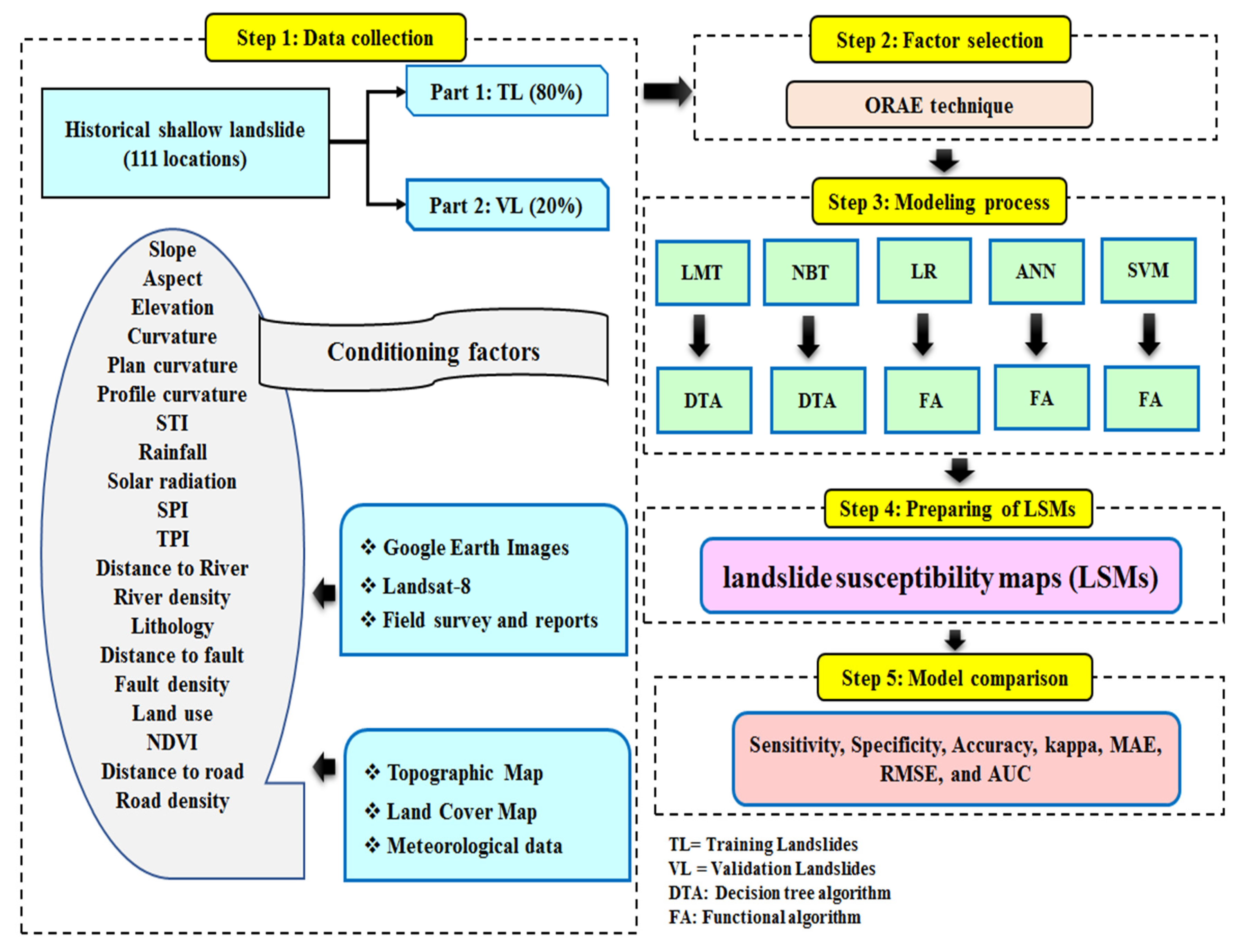
4.8. Summary of the Methodology Used in This Study

Figure 5 provides a summary of the methodology used in our study. In this study, we prepared and used of the following steps for the modeling process and for preparing shallow landslide susceptibility maps:

Step 1: Data collection

We first created the landslide inventory map and selected possible landslide conditioning factors (Section 3.2, respectively, of this paper).

Step 2: Factor selection

We next used the ORAE feature selection technique to select the most important factors for landslide occurrence in the study area (Section 4.7).

Step 3: Modelling process

We next applied the LMT, NBT, LR, ANN, and SVM machine learning models using the most important factors determined in step 2 (Section 4.1, Section 4.2, Section 4.3, Section 4.4 and Section 4.5).

Step 4: Preparation of shallow landslide susceptibility maps

We applied each model to the training dataset and calculated a weight (shallow landslide susceptibility index) for each pixel of the study area. Based on these weights, we created shallow landslide susceptibility maps.

Step 5: Model comparison and validation

We used statistical indexes, namely sensitivity, specificity, accuracy, MAE, RMSE, and AUC, to check goodness-of-fit and prediction power using, respectively, the training and validation datasets (Section 4.6.1 and Section 4.6.2). Additionally, we tested the results using the Freidman and Wilcoxon statistical tests (Section 4.6.3).

5. Results and Analysis

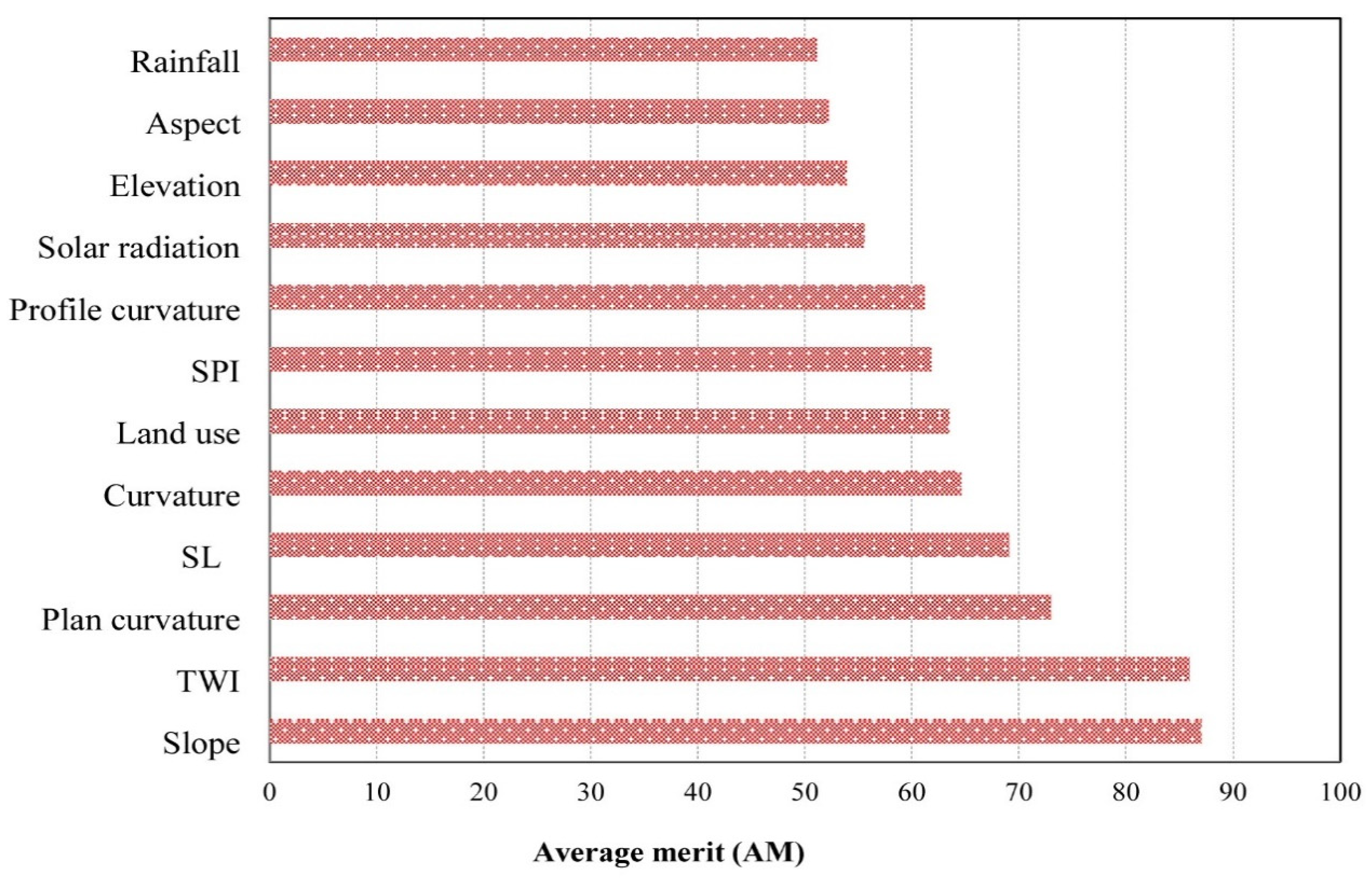
5.1. Most Important Landslide Conditioning Factors

Using the ORAE method, we found that 12 of the 20 candidate conditioning factors had adequate predictive ability (AM > 0) to be used in modeling landslide susceptibility. The average merit, based on a 10-fold cross validation technique, is illustrated in Figure 6. Slope angle and TWI had the highest average merits (respectively, 87.08 and 85.96), followed by plan curvature (73.03), slope length (69.10), curvature (64.61), land use (63.48), SPI (61.80), profile curvature (61.24), solar radiation (55.62), elevation (53.93), aspect (52.25), and rainfall (51.12).

5.2. Model Performance and Analysis

The performances of the applied predictive models (LMT, NBT, LR, ANN, and SVM) were determined based on both the training and validation datasets (

Table 1. Model performances of the applied data-mining approaches for the training and validation datasets.

Parameters	LMT		NBT		LR		ANN		SVM
	T *	V *	T	V	T	V	T	V	T	V
True positive	78	19	77	18	80	19	76	16	77	18
True negative	81	19	83	20	81	19	73	17	83	20
False positive	11	3	12	4	9	3	13	6	12	4
False negative	8	3	6	2	8	3	16	5	6	2
Sensitivity (%)	0.907	0.864	0.928	0.900	0.909	0.864	0.826	0.762	0.928	0.900
Specificity (%)	0.880	0.864	0.874	0.833	0.900	0.864	0.849	0.739	0.874	0.833
Accuracy (%)	0.893	0.864	0.899	0.864	0.904	0.864	0.837	0.750	0.899	0.864
MAE	0.207	0.216	0.225	0.225	0.213	0.216	0.241	0.235	0.223	0.246
RMSE	0.304	0.313	0.319	0.341	0.311	0.314	0.349	0.358	0.318	0.369
AUC	0.944	0.936	0.918	0.874	0.939	0.936	0.911	0.871	0.899	0.864

T *: Training, V *: Validation.

). In the case of the training dataset, the LMT model achieved the best goodness-of-fit, as quantified by MAE (0.207), RMSE (0.304), and AUC (0.944). The NBT and SVM models have the highest sensitivity (0.928), and the LR model has the best specificity (0.900) and accuracy (0.904). The NBT and SVM models have the best quality, with 92.8% of the landslide pixels properly assigned to the landslide class, followed by LR (90.9%), LMT (90.7%), and ANN (82.6%). The LR model has the highest specificity, with 90.0% of the no-landslide pixels properly classified in the no-landslide class. This model also has the best accuracy, with a 90.4% probability of properly categorized pixels, followed by the NBT and SVM (89.9%), LMT (89.3%), and ANN (83.7%) models.

For the validation dataset, both the LMT and LR models have the highest goodness-of-fit based on the MAE (0.216), RMSE (0.313 and 0.314), and AUC (0.936) measures, followed by the NBT model. The NBT model also has the best sensitivity, with 90.0% of the landslide pixels in the correct class. The LMT and LR models have the highest specificity (0.864), with 86.4% of non-landslide pixels in the right class. The next highest specificity (0.833) was obtained by the NBT and SVM models. In terms of accuracy, all of the predictive models except ANN have the same accuracy (0.864), indicating that the probability of pixels being correctly categorized is 86.4%. It is worth noting that ANN has the lowest values for sensitivity (0.762), specificity (0.739), and accuracy (0.750), and that SVM has the lowest goodness-of-fit based on the MAE (0.246), RMSE (0.369), and AUC (0.864) measures.

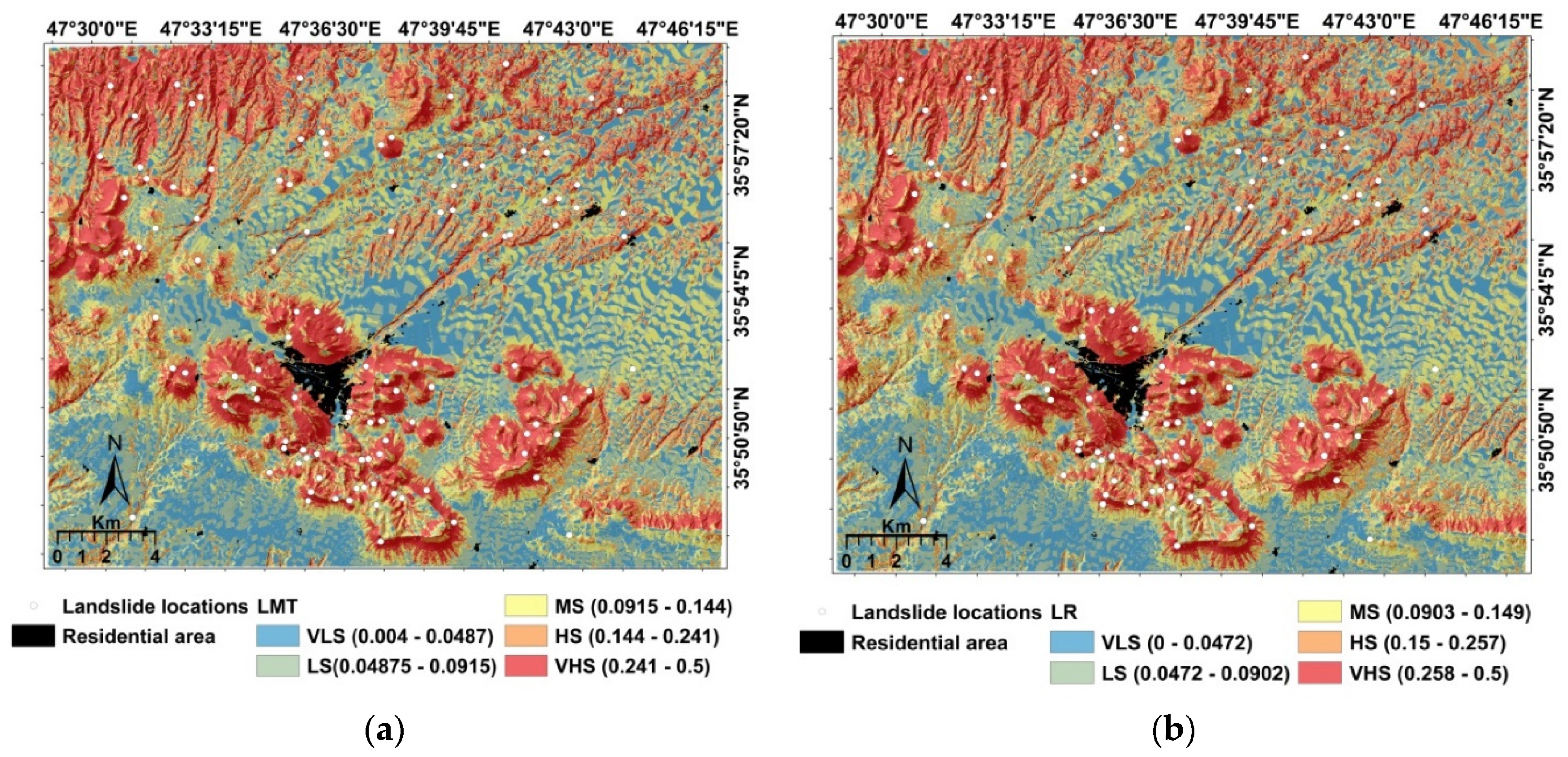
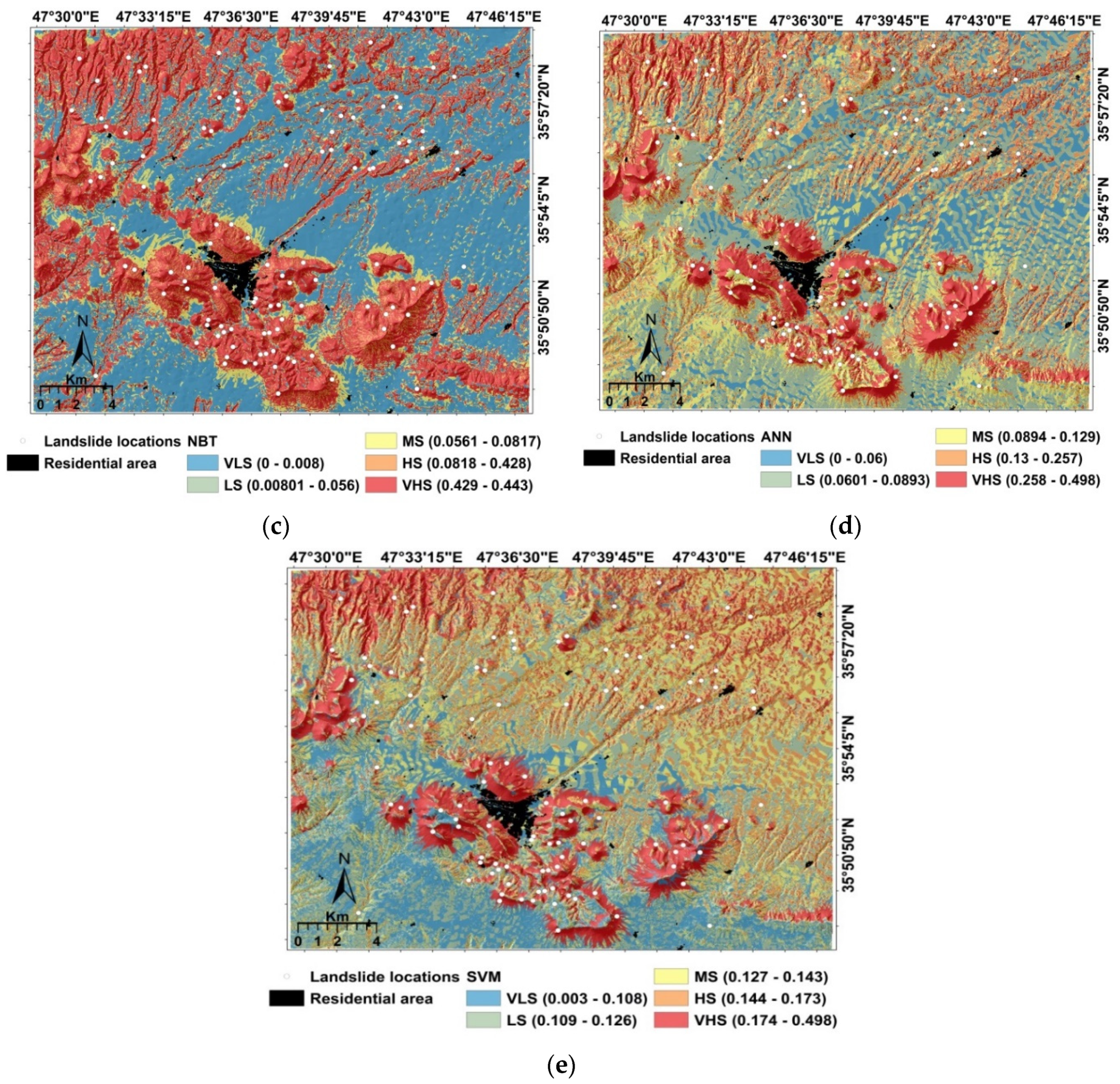
5.3. Development of Landslide Susceptibility Maps

After developing the LMT, LR, NBT, ANN, and SVM models, we estimated landslide susceptibility indices (LSI) for each pixel in each model. LSIs were computed according to the probability distribution function of each model. In order to facilitate the visualization of the susceptibility models, we divided the indices into five susceptibility classes by the natural break method: very low (VLS), low (LS), moderate (MS), high (HS), and very high (VHS). Finally, we developed a susceptibility map for each of the five models (Figure 7). These maps consistently indicate that the south-central and northwestern parts of the study area, which are hilly and mountainous, are most susceptible to landslides.

5.4. Model Comparison and Validation

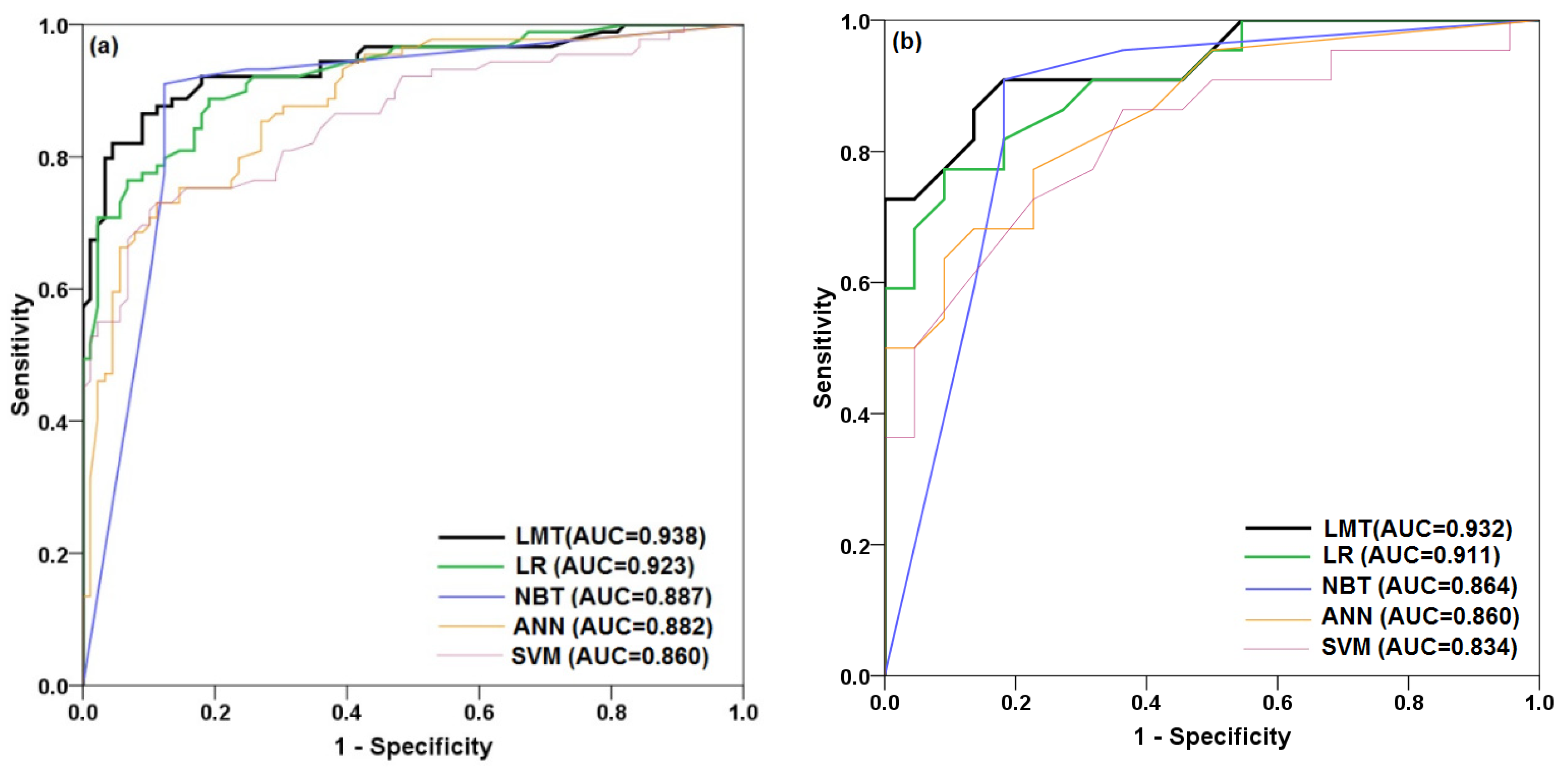
5.4.1. ROC Curve

We evaluated the validity of the shallow landslide susceptibility maps based on the ROC curves and AUC values (Figure 8). The area under the curve for the training dataset is largest for the LMT model (0.938), followed by the LR (0.923), NBT (0.887), ANN (0.882), and SVM (0.860) models (Figure 8a). The area under the curve for the validation dataset is also highest for the LMT model (0.932), followed by the LR (0.911), NBT (0.864), ANN (0.860), and SVM (0.834) models (Figure 8b). These values suggest that the LMT model has the highest goodness-of-fit and prediction accuracy for the study area. Overall, the results indicate that the LMT classifier provides a higher quality landslide susceptibility model for the study area than the other machine learning methods.

5.4.2. Wilcoxon Sign Rank Test

In addition to ROC, the statistical treatments of the five machine learning models were also analyzed by two well-known non-parametric statistical tests including the Friedman and Wilcoxon tests. As abovementioned, the null hypothesis is rejected if the significant level of a model is less than 0.05 (α = 0.05). The null hypothesis that there is no difference among the performances of the shallow landslide models at a significance level of α = 0.05 (5%) was rejected. In this case, it was concluded that two or more model are statistically different in terms of performance. The result of the Friedman test concluded that the significant value was less than 0.05 and hence the null hypothesis was rejected (true). The Friedman method, however, provides no information on pairwise comparison. The Wilcoxon test assessed systematic pairwise differences among the shallow landslide models and indicated significant differences among some of them (

Table 2. Performance of the five landslide machine learning models using Wilcoxon signed-rank test (two-tailed).

No.	Landslide Model	Mean Rank	χ2	p-Value
1	LMT	2.80	557.912	0.000
2	LR	2.93
3	NBT	2.88
4	ANN	3.07
5	SVM	2.32

). There was no significant difference between the LMT and LR models, indicating that these two algorithms have similar predictive power. In contrast, the performances of the other models were significantly different from each other, and from the LMT and LR (

Table 3. Performance of the five landslide machine learning models using the Wilcoxon signed-rank test (two-tailed).

No.	Pairwise Comparison	Number of Positive Differences	Number of Negative Differences	z-Value	p-Value	Significance
1	LMT vs. LR	60	50	−1.536	0.125	No
2	LMT vs. NBT	83	27	−5.590	0.000	Yes
3	LMT vs. ANN	62	46	−0.878	0.080	Yes
4	LMT vs. SVM	36	74	−3.677	0.000	Yes
5	LR vs. NBT	82	29	−5.589	0.000	Yes
6	LR vs. ANN	61	49	−0.605	0.015	Yes
7	LR vs. SVM	35	75	−4.081	0.000	Yes
8	NBT vs. ANN	36	73	−3.958	0.000	Yes
9	NBT vs. SVM	30	80	−5.711	0.000	Yes
10	ANN vs. SVM	43	67	−3.140	0.002	Yes

Note: The standard p-value is 0.05.

).

6. Discussion

The ability to accurately estimate the sensitivity of terrain to landslides is an essential step in land-use planning [158]. Integration of advanced machine learning algorithms now allows researchers to develop landslide susceptibility models with high predictive capabilities. Land-use planners can use maps produced from these models to reduce landslide risk [159]. However, many different methods for modeling landslide sensitivity have been proposed, and the predictive accuracy of these methods continues to be debated [160]. The growth in computer processing power offers researchers new opportunities to compare models and evaluate their advantages and disadvantages.

Among the issues faced by researchers is the selection of appropriate landslide conditioning factors. Appropriate conditioning factors may differ from region to region, depending on geology, soils, topography, climate, and land use [161]. Thus, protocols must be developed to test the predictive ability of the entire suite of factors that are under consideration [162,163]. In this study, we prepared a landslide inventory map comprising 111 landslides and considered 20 conditioning factors. We used the ORAE method and the AM index to remove 12 of the 20 factors from the landslide modeling process. Slope has the highest average merits and is deemed to be the most critical factor in determining landslide susceptibility in the Bijar study area. Landslides in this area are most common on the steep, relatively wet slopes with sparse vegetation [54,164].

In this study, we compared the performance of five machine learning models: Logistic Model Tree, Logistic Regression, Naive Bayes Tree, Artificial Neural Network, and Support Vector Machine. All five models performed well, with classification accuracies >0.837 for the training dataset and 0.75 for the validation dataset. Model validation was performed using several statistical indices, for example accuracy and ROC. The LMT model provided the best balance of classification capability and performance. The LMT model uses leaf nodes and does not use constant values [161]. And according to Landwehr et al. [132], LMT is efficient in constructing logistic models at lower levels of the tree, rather than extending to lower levels models already established at higher levels. Moreover, the LMT algorithm applies cross-validation of LogitBoost iterations because training samples may be incorrectly modified. The LMT model was validated with statistical measures and ROC.

The LR, ANN, and SVM models require much more computer power and lengthy execution times. Typically, data are converted to ASCII format for statistical analysis and are later reformatted for integration into a GIS. In addition, processing of large amounts of data in the statistical package is more complicated for these three models [139,165,166]. A disadvantage of the NBT model is the assumption that it does not depend on the attribution. Research by Tien Bui et al. [22] suggests that this assumption may be incorrect, at least in the case of landslides.

We argue that the LMT model is an effective and simple tool for landslide susceptibility mapping. We acknowledge, however, that there is no consensus about the best method for modeling landslide susceptibility. In this paper, we compared five techniques: Logistic Model Tree, Logistic Regression, Naive Bayes Tree, Artificial Neural Network, and Support Vector Machine to evaluate landslide susceptibility in a semi-arid area in northwestern Iran. It is noted that all five methods perform well, but the LMT model is superior.

The proposed approach has advantages as well as limitations. The advantages are: (1) it has established and applied rules that are extractable and understandable; (2) it makes pair-wise comparisons; (3) it is structured to work quickly with large and complex datasets; (4) it can detect relationships and differences in subgroups and adjust for missing data; and (5) it does not rely on expert knowledge and experience to make decisions. However, it is limited by the available database and the choice of landslide conditioning factors. Small samples pose major obstacles. Future research should aim to find ways to reduce the small dataset problem, for example by replacing landslide points with landslide polygons which would significantly increase the number of pixels and improve the quality of models.

7. Conclusions

Accurate landslide susceptibility maps assist land-use planners and government officials to reduce loss of life and damage from slope failures. In this study, we prepared landslide susceptibility maps for the area around Bijar City, Iran, using five soft-computing benchmark algorithms: LMT, LR, NBT, ANN, and SVM. Our database comprised 111 shallow landslides. We divided the landslides into training and prediction groups and selected 20 landslide conditioning factors for modeling based on the Information Gain Ratio technique. All data were elaborated in a GIS environment. We determined that slope angle and the topographic wetness index are the most important factors for shallow landslide occurrence in the study area. The hilly and mountainous parts of the study area have a higher likelihood of shallow landslides, especially if their soils are saturated.

Although all five machine learning models performed well, the LMT model outperformed the others. It thus has considerable promise as a tool for mapping shallow landslide susceptibility in other semi-arid regions with similar topography, geology, and climate. We recommend it as a tool to help planners, managers, and government agencies mitigate landslide hazards. The LR model outperformed the NBT, ANN, and SVM models, thus we consider it to be a trustworthy model for identifying shallow landslide-prone areas in semi-arid environments.

A long-term goal of landslide researchers is the development of protocols for producing accurate landslide susceptibility maps. Many hurdles remain before this is possible, including limitations in available data, unknown factors, and known factors that are dynamic in nature (e.g., temporal changes in climate and land use). Thus, much more research is needed, and we advise caution in generalizing results in one area to others.

References

1. Klose, M.; Maurischat, P.; Damm, B. Landslide impacts in Germany: A historical and socioeconomic perspective. Landslides 2016, 13, 183–199. [Google Scholar] [CrossRef]
2. Dilley, M.; Chen, R.S.; Deichmann, U.; Lerner-Lam, A.L.; Arnold, M. Natural Disaster Hotspots: A Global Risk Analysis; The World Bank: Washington, DC, USA, 2005. [Google Scholar]
3. Gariano, S.L.; Sarkar, R.; Dikshit, A.; Dorji, K.; Brunetti, M.T.; Peruccacci, S.; Melillo, M. Automatic calculation of rainfall thresholds for landslide occurrence in Chukha Dzongkhag, Bhutan. Bull. Eng. Geol. Environ. 2019, 78, 4325–4332. [Google Scholar] [CrossRef]
4. Dikshit, A.; Sarkar, R.; Pradhan, B.; Acharya, S.; Dorji, K. Estimating rainfall thresholds for landslide occurrence in the Bhutan Himalayas. Water 2019, 11, 1616. [Google Scholar] [CrossRef] [Green Version]
5. Froude, M.J.; Petley, D. Global fatal landslide occurrence from 2004 to 2016. Nat. Hazards Earth Syst. Sci. 2018, 18, 2161–2181. [Google Scholar] [CrossRef] [Green Version]
6. Cruden, D. A suggested method for a landslide summary. Bull. Int. Assoc. Eng. Geol. -Bull. De L’association Int. De Géologie De L’ingénieur 1991, 43, 101–110. [Google Scholar]
7. Farrokhnia, A.; Pirasteh, S.; Pradhan, B.; Pourkermani, M.; Arian, M. A recent scenario of mass wasting and its impact on the transportation in Alborz Mountains, Iran using geo-information technology. Arab. J. Geosci. 2011, 4, 1337–1349. [Google Scholar] [CrossRef]
8. Ayazi, M.H.; Pirasteh, S.; Arvin, A.; Pradhan, B.; Nikouravan, B.; Mansor, S. Disasters and risk reduction in groundwater: Zagros mountain southwest Iran using geoinformatics techniques. Disaster Adv. 2010, 3, 51–57. [Google Scholar]
9. Safari, H.O.; Pirasteh, S.; Pradhan, B. Upliftment estimation of the Zagros transverse fault in Iran using geoinformatics technology. Remote Sens. 2009, 1, 1240–1256. [Google Scholar] [CrossRef] [Green Version]
10. Akbarimehr, M.; Motagh, M.; Haghshenas-Haghighi, M. Slope stability assessment of the Sarcheshmeh landslide, northeast Iran, investigated using INSAR and GPS observations. Remote Sens. 2013, 5, 3681–3700. [Google Scholar] [CrossRef] [Green Version]
11. Talaei, R.; Samadov, S. Quantitative landslide risk analysis in the Hashtchin area (NW-Iran). Eur. J. Environ. Civ. Eng. 2018, 22, 883–909. [Google Scholar] [CrossRef]
12. Dou, J.; Yunus, A.P.; Merghadi, A.; Shirzadi, A.; Nguyen, H.; Hussain, Y.; Avtar, R.; Chen, Y.; Pham, B.T.; Yamagishi, H. Different sampling strategies for predicting landslide susceptibilities are deemed less consequential with deep learning. Sci. Total Environ. 2020, 720, 137–153. [Google Scholar] [CrossRef]
13. Pham, B.T.; Jaafari, A.; Prakash, I.; Bui, D.T. A novel hybrid intelligent model of support vector machines and the MultiBoost ensemble for landslide susceptibility modeling. Bull. Eng. Geol. Environ. 2019, 78, 2865–2886. [Google Scholar] [CrossRef]
14. Brabb, E.E. Innovative approaches to landslide hazard and risk mapping. In Proceedings of the International Landslide Symposium Proceedings, Toronto, ON, Canada, 23–31 August 1985; pp. 17–22. [Google Scholar]
15. Guzzetti, F.; Reichenbach, P.; Cardinali, M.; Galli, M.; Ardizzone, F. Probabilistic landslide hazard assessment at the basin scale. Geomorphology 2005, 72, 272–299. [Google Scholar] [CrossRef]
16. Dikshit, A.; Sarkar, R.; Pradhan, B.; Jena, R.; Drukpa, D.; Alamri, A.M. Temporal probability assessment and its use in landslide susceptibility mapping for eastern Bhutan. Water 2020, 12, 267. [Google Scholar] [CrossRef] [Green Version]
17. Shirzadi, A.; Bui, D.T.; Pham, B.T.; Solaimani, K.; Chapi, K.; Kavian, A.; Shahabi, H.; Revhaug, I. Shallow landslide susceptibility assessment using a novel hybrid intelligence approach. Environ. Earth Sci. 2017, 76, 60. [Google Scholar] [CrossRef]
18. Pham, B.T.; Prakash, I.; Singh, S.K.; Shirzadi, A.; Shahabi, H.; Bui, D.T. Landslide susceptibility modeling using reduced error pruning trees and different ensemble techniques: Hybrid machine learning approaches. Catena 2019, 175, 203–218. [Google Scholar] [CrossRef]
19. Pourghasemi, H.R.; Yansari, Z.T.; Panagos, P.; Pradhan, B. Analysis and evaluation of landslide susceptibility: A review on articles published during 2005–2016 (periods of 2005–2012 and 2013–2016). Arab. J. Geosci. 2018, 11, 193. [Google Scholar] [CrossRef]
20. Bai, S.-B.; Wang, J.; Lü, G.-N.; Zhou, P.-G.; Hou, S.-S.; Xu, S.-N. Gis-based logistic regression for landslide susceptibility mapping of the zhongxian segment in the three gorges area, China. Geomorphology 2010, 115, 23–31. [Google Scholar] [CrossRef]
21. Atkinsson, P.; Massari, R. Generalized linear modeling of susceptibility to landsliding in the central Appennines, Italy. Comput. Geosci. 1998, 24, 373–385. [Google Scholar] [CrossRef]
22. Bui, D.T.; Tuan, T.A.; Klempe, H.; Pradhan, B.; Revhaug, I. Spatial prediction models for shallow landslide hazards: A comparative assessment of the efficacy of support vector machines, artificial neural networks, kernel logistic regression, and logistic model tree. Landslides 2016, 13, 361–378. [Google Scholar]
23. Wang, Y.; Hong, H.; Chen, W.; Li, S.; Panahi, M.; Khosravi, K.; Shirzadi, A.; Shahabi, H.; Panahi, S.; Costache, R. Flood susceptibility mapping in Dingnan county (China) using adaptive neuro-fuzzy inference system with biogeography based optimization and imperialistic competitive algorithm. J. Environ. Manag. 2019, 247, 712–729. [Google Scholar] [CrossRef] [PubMed]
24. Khosravi, K.; Shahabi, H.; Pham, B.T.; Adamowski, J.; Shirzadi, A.; Pradhan, B.; Dou, J.; Ly, H.-B.; Gróf, G.; Ho, H.L. A comparative assessment of flood susceptibility modeling using multi-criteria decision-making analysis and machine learning methods. J. Hydrol. 2019, 573, 311–323. [Google Scholar] [CrossRef]
25. Chen, W.; Hong, H.; Li, S.; Shahabi, H.; Wang, Y.; Wang, X.; Ahmad, B.B. Flood susceptibility modelling using novel hybrid approach of reduced-error pruning trees with bagging and random subspace ensembles. J. Hydrol. 2019, 575, 864–873. [Google Scholar] [CrossRef]
26. Tien Bui, D.; Shirzadi, A.; Chapi, K.; Shahabi, H.; Pradhan, B.; Pham, B.T.; Singh, V.P.; Chen, W.; Khosravi, K.; Bin Ahmad, B. A hybrid computational intelligence approach to groundwater spring potential mapping. Water 2019, 11, 2013. [Google Scholar] [CrossRef] [Green Version]
27. Bui, D.T.; Panahi, M.; Shahabi, H.; Singh, V.P.; Shirzadi, A.; Chapi, K.; Khosravi, K.; Chen, W.; Panahi, S.; Li, S. Novel hybrid evolutionary algorithms for spatial prediction of floods. Sci. Rep. 2018, 8, 15364. [Google Scholar] [CrossRef] [Green Version]
28. Tien Bui, D.; Khosravi, K.; Li, S.; Shahabi, H.; Panahi, M.; Singh, V.; Chapi, K.; Shirzadi, A.; Panahi, S.; Chen, W. New hybrids of ANFIS with several optimization algorithms for flood susceptibility modeling. Water 2018, 10, 1210. [Google Scholar] [CrossRef] [Green Version]
29. Shafizadeh-Moghadam, H.; Valavi, R.; Shahabi, H.; Chapi, K.; Shirzadi, A. Novel forecasting approaches using combination of machine learning and statistical models for flood susceptibility mapping. J. Environ. Manag. 2018, 217, 1–11. [Google Scholar] [CrossRef] [Green Version]
30. Chapi, K.; Singh, V.P.; Shirzadi, A.; Shahabi, H.; Bui, D.T.; Pham, B.T.; Khosravi, K. A novel hybrid artificial intelligence approach for flood susceptibility assessment. Environ. Model. Softw. 2017, 95, 229–245. [Google Scholar] [CrossRef]
31. Chen, W.; Li, Y.; Xue, W.; Shahabi, H.; Li, S.; Hong, H.; Wang, X.; Bian, H.; Zhang, S.; Pradhan, B. Modeling flood susceptibility using data-driven approaches of naïve bayes tree, alternating decision tree, and random forest methods. Sci. Total Environ. 2020, 701, 134979. [Google Scholar] [CrossRef]
32. Shahabi, H.; Shirzadi, A.; Ghaderi, K.; Omidvar, E.; Al-Ansari, N.; Clague, J.J.; Geertsema, M.; Khosravi, K.; Amini, A.; Bahrami, S. Flood detection and susceptibility mapping using Sentinel-1 remote sensing data and a machine learning approach: Hybrid intelligence of bagging ensemble based on k-nearest neighbor classifier. Remote Sens. 2020, 12, 266. [Google Scholar] [CrossRef] [Green Version]
33. Khosravi, K.; Melesse, A.M.; Shahabi, H.; Shirzadi, A.; Chapi, K.; Hong, H. Flood susceptibility mapping at ningdu catchment, china using bivariate and data mining techniques. In Extreme Hydrology and Climate Variability; Elsevier: Amsterdam, The Netherlands, 2019; pp. 419–434. [Google Scholar]
34. Jaafari, A.; Termeh, S.V.R.; Bui, D.T. Genetic and firefly metaheuristic algorithms for an optimized neuro-fuzzy prediction modeling of wildfire probability. J. Environ. Manag. 2019, 243, 358–369. [Google Scholar] [CrossRef] [PubMed]
35. Hong, H.; Jaafari, A.; Zenner, E.K. Predicting spatial patterns of wildfire susceptibility in the huichang county, china: An integrated model to analysis of landscape indicators. Ecol. Indic. 2019, 101, 878–891. [Google Scholar] [CrossRef]
36. Rahmati, O.; Panahi, M.; Ghiasi, S.S.; Deo, R.C.; Tiefenbacher, J.P.; Pradhan, B.; Jahani, A.; Goshtasb, H.; Kornejady, A.; Shahabi, H. Hybridized neural fuzzy ensembles for dust source modeling and prediction. Atmos. Environ. 2020, 224, 117320. [Google Scholar] [CrossRef]
37. Taheri, K.; Shahabi, H.; Chapi, K.; Shirzadi, A.; Gutiérrez, F.; Khosravi, K. Sinkhole susceptibility mapping: A comparison between bayes-based machine learning algorithms. Land Degrad. Dev. 2019, 30, 730–745. [Google Scholar] [CrossRef]
38. Roodposhti, M.S.; Safarrad, T.; Shahabi, H. Drought sensitivity mapping using two one-class support vector machine algorithms. Atmos. Res. 2017, 193, 73–82. [Google Scholar] [CrossRef]
39. Choubin, B.; Soleimani, F.; Pirnia, A.; Sajedi-Hosseini, F.; Alilou, H.; Rahmati, O.; Melesse, A.M.; Singh, V.P.; Shahabi, H. Effects of drought on vegetative cover changes: Investigating spatiotemporal patterns. In Extreme Hydrology and Climate Variability; Elsevier: Amsterdam, The Netherlands, 2019; pp. 213–222. [Google Scholar]
40. Lee, S.; Panahi, M.; Pourghasemi, H.R.; Shahabi, H.; Alizadeh, M.; Shirzadi, A.; Khosravi, K.; Melesse, A.M.; Yekrangnia, M.; Rezaie, F. Sevucas: A novel gis-based machine learning software for seismic vulnerability assessment. Appl. Sci. 2019, 9, 3495. [Google Scholar] [CrossRef] [Green Version]
41. Alizadeh, M.; Alizadeh, E.; Asadollahpour Kotenaee, S.; Shahabi, H.; Beiranvand Pour, A.; Panahi, M.; Bin Ahmad, B.; Saro, L. Social vulnerability assessment using artificial neural network (ANN) model for earthquake hazard in Tabriz City, Iran. Sustainability 2018, 10, 3376. [Google Scholar] [CrossRef] [Green Version]
42. Azareh, A.; Rahmati, O.; Rafiei-Sardooi, E.; Sankey, J.B.; Lee, S.; Shahabi, H.; Ahmad, B.B. Modelling gully-erosion susceptibility in a semi-arid region, Iran: Investigation of applicability of certainty factor and maximum entropy models. Sci. Total Environ. 2019, 655, 684–696. [Google Scholar] [CrossRef]
43. Tien Bui, D.; Shirzadi, A.; Shahabi, H.; Chapi, K.; Omidavr, E.; Pham, B.T.; Talebpour Asl, D.; Khaledian, H.; Pradhan, B.; Panahi, M. A novel ensemble artificial intelligence approach for gully erosion mapping in a semi-arid watershed (Iran). Sensors 2019, 19, 2444. [Google Scholar] [CrossRef] [Green Version]
44. Nhu, V.-H.; Janizadeh, S.; Avand, M.; Chen, W.; Farzin, M.; Omidvar, E.; Shirzadi, A.; Shahabi, H.; Clague, J.J.; Jaafari, A. Gis-based gully erosion susceptibility mapping: A comparison of computational ensemble data mining models. Appl. Sci. 2020, 10, 2039. [Google Scholar] [CrossRef] [Green Version]
45. Tien Bui, D.; Shahabi, H.; Shirzadi, A.; Chapi, K.; Pradhan, B.; Chen, W.; Khosravi, K.; Panahi, M.; Bin Ahmad, B.; Saro, L. Land subsidence susceptibility mapping in south Korea using machine learning algorithms. Sensors 2018, 18, 2464. [Google Scholar] [CrossRef] [PubMed] [Green Version]
46. Rahmati, O.; Samadi, M.; Shahabi, H.; Azareh, A.; Rafiei-Sardooi, E.; Alilou, H.; Melesse, A.M.; Pradhan, B.; Chapi, K.; Shirzadi, A. Swpt: An automated gis-based tool for prioritization of sub-watersheds based on morphometric and topo-hydrological factors. Geosci. Front. 2019, 10, 2167–2175. [Google Scholar] [CrossRef]
47. Rahmati, O.; Choubin, B.; Fathabadi, A.; Coulon, F.; Soltani, E.; Shahabi, H.; Mollaefar, E.; Tiefenbacher, J.; Cipullo, S.; Ahmad, B.B. Predicting uncertainty of machine learning models for modelling nitrate pollution of groundwater using quantile regression and uneec methods. Sci. Total Environ. 2019, 688, 855–866. [Google Scholar] [CrossRef] [PubMed]
48. Chen, W.; Pradhan, B.; Li, S.; Shahabi, H.; Rizeei, H.M.; Hou, E.; Wang, S. Novel hybrid integration approach of bagging-based fisher’s linear discriminant function for groundwater potential analysis. Nat. Resour. Res. 2019, 28, 1239–1258. [Google Scholar] [CrossRef] [Green Version]
49. Miraki, S.; Zanganeh, S.H.; Chapi, K.; Singh, V.P.; Shirzadi, A.; Shahabi, H.; Pham, B.T. Mapping groundwater potential using a novel hybrid intelligence approach. Water Resour. Manag. 2019, 33, 281–302. [Google Scholar] [CrossRef]
50. Rahmati, O.; Naghibi, S.A.; Shahabi, H.; Bui, D.T.; Pradhan, B.; Azareh, A.; Rafiei-Sardooi, E.; Samani, A.N.; Melesse, A.M. Groundwater spring potential modelling: Comprising the capability and robustness of three different modeling approaches. J. Hydrol. 2018, 565, 248–261. [Google Scholar] [CrossRef]
51. Chen, W.; Li, Y.; Tsangaratos, P.; Shahabi, H.; Ilia, I.; Xue, W.; Bian, H. Groundwater spring potential mapping using artificial intelligence approach based on kernel logistic regression, random forest, and alternating decision tree models. Appl. Sci. 2020, 10, 425. [Google Scholar] [CrossRef] [Green Version]
52. Tien Bui, D.; Shahabi, H.; Shirzadi, A.; Chapi, K.; Alizadeh, M.; Chen, W.; Mohammadi, A.; Ahmad, B.; Panahi, M.; Hong, H. Landslide detection and susceptibility mapping by AIRSAR data using support vector machine and index of entropy models in Cameron Highlands, Malaysia. Remote Sens. 2018, 10, 1527. [Google Scholar] [CrossRef] [Green Version]
53. Chen, W.; Peng, J.; Hong, H.; Shahabi, H.; Pradhan, B.; Liu, J.; Zhu, A.-X.; Pei, X.; Duan, Z. Landslide susceptibility modelling using GIS-based machine learning techniques for Chongren county, Jiangxi province, China. Sci. Total Environ. 2018, 626, 1121–1135. [Google Scholar] [CrossRef]
54. Pham, B.T.; Shirzadi, A.; Shahabi, H.; Omidvar, E.; Singh, S.K.; Sahana, M.; Asl, D.T.; Ahmad, B.B.; Quoc, N.K.; Lee, S. Landslide susceptibility assessment by novel hybrid machine learning algorithms. Sustainability 2019, 11, 4386. [Google Scholar] [CrossRef] [Green Version]
55. Pham, B.T.; Prakash, I.; Dou, J.; Singh, S.K.; Trinh, P.T.; Tran, H.T.; Le, T.M.; Van Phong, T.; Khoi, D.K.; Shirzadi, A. A novel hybrid approach of landslide susceptibility modelling using rotation forest ensemble and different base classifiers. Geocarto Int. 2019, 1–25. [Google Scholar] [CrossRef]
56. Pradhan, B. A comparative study on the predictive ability of the decision tree, support vector machine and neuro-fuzzy models in landslide susceptibility mapping using GIS. Comput. Geosci. 2013, 51, 350–365. [Google Scholar] [CrossRef]
57. Chen, W.; Shahabi, H.; Shirzadi, A.; Hong, H.; Akgun, A.; Tian, Y.; Liu, J.; Zhu, A.-X.; Li, S. Novel hybrid artificial intelligence approach of bivariate statistical-methods-based kernel logistic regression classifier for landslide susceptibility modeling. Bull. Eng. Geol. Environ. 2019, 78, 4397–4419. [Google Scholar] [CrossRef]
58. He, Q.; Shahabi, H.; Shirzadi, A.; Li, S.; Chen, W.; Wang, N.; Chai, H.; Bian, H.; Ma, J.; Chen, Y. Landslide spatial modelling using novel bivariate statistical based naïve bayes, RBF classifier, and RBF network machine learning algorithms. Sci. Total Environ. 2019, 663, 1–15. [Google Scholar] [CrossRef] [PubMed]
59. Jaafari, A.; Panahi, M.; Pham, B.T.; Shahabi, H.; Bui, D.T.; Rezaie, F.; Lee, S. Meta optimization of an adaptive neuro-fuzzy inference system with grey wolf optimizer and biogeography-based optimization algorithms for spatial prediction of landslide susceptibility. Catena 2019, 175, 430–445. [Google Scholar] [CrossRef]
60. Hong, H.; Shahabi, H.; Shirzadi, A.; Chen, W.; Chapi, K.; Ahmad, B.B.; Roodposhti, M.S.; Hesar, A.Y.; Tian, Y.; Bui, D.T. Landslide susceptibility assessment at the Wuning area, China: A comparison between multi-criteria decision making, bivariate statistical and machine learning methods. Nat. Hazards 2019, 96, 173–212. [Google Scholar] [CrossRef]
61. Shafizadeh-Moghadam, H.; Minaei, M.; Shahabi, H.; Hagenauer, J. Big data in geohazard; pattern mining and large scale analysis of landslides in Iran. Earth Sci. Inform. 2019, 12, 1–17. [Google Scholar] [CrossRef]
62. Nguyen, V.V.; Pham, B.T.; Vu, B.T.; Prakash, I.; Jha, S.; Shahabi, H.; Shirzadi, A.; Ba, D.N.; Kumar, R.; Chatterjee, J.M. Hybrid machine learning approaches for landslide susceptibility modeling. Forests 2019, 10, 157. [Google Scholar] [CrossRef] [Green Version]
63. Nguyen, P.T.; Tuyen, T.T.; Shirzadi, A.; Pham, B.T.; Shahabi, H.; Omidvar, E.; Amini, A.; Entezami, H.; Prakash, I.; Phong, T.V. Development of a novel hybrid intelligence approach for landslide spatial prediction. Appl. Sci. 2019, 9, 2824. [Google Scholar] [CrossRef] [Green Version]
64. Tien Bui, D.; Shahabi, H.; Omidvar, E.; Shirzadi, A.; Geertsema, M.; Clague, J.J.; Khosravi, K.; Pradhan, B.; Pham, B.T.; Chapi, K. Shallow landslide prediction using a novel hybrid functional machine learning algorithm. Remote Sens. 2019, 11, 931. [Google Scholar] [CrossRef] [Green Version]
65. Tien Bui, D.; Shirzadi, A.; Shahabi, H.; Geertsema, M.; Omidvar, E.; Clague, J.J.; Thai Pham, B.; Dou, J.; Talebpour Asl, D.; Bin Ahmad, B. New ensemble models for shallow landslide susceptibility modeling in a semi-arid watershed. Forests 2019, 10, 743. [Google Scholar] [CrossRef] [Green Version]
66. Chen, W.; Zhao, X.; Shahabi, H.; Shirzadi, A.; Khosravi, K.; Chai, H.; Zhang, S.; Zhang, L.; Ma, J.; Chen, Y. Spatial prediction of landslide susceptibility by combining evidential belief function, logistic regression and logistic model tree. Geocarto Int. 2019, 34, 1177–1201. [Google Scholar] [CrossRef]
67. Shirzadi, A.; Solaimani, K.; Roshan, M.H.; Kavian, A.; Chapi, K.; Shahabi, H.; Keesstra, S.; Ahmad, B.B.; Bui, D.T. Uncertainties of prediction accuracy in shallow landslide modeling: Sample size and raster resolution. Catena 2019, 178, 172–188. [Google Scholar] [CrossRef]
68. Tien Bui, D.; Shahabi, H.; Shirzadi, A.; Chapi, K.; Hoang, N.-D.; Pham, B.; Bui, Q.-T.; Tran, C.-T.; Panahi, M.; Bin Ahamd, B. A novel integrated approach of relevance vector machine optimized by imperialist competitive algorithm for spatial modeling of shallow landslides. Remote Sens. 2018, 10, 1538. [Google Scholar] [CrossRef] [Green Version]
69. Shirzadi, A.; Soliamani, K.; Habibnejhad, M.; Kavian, A.; Chapi, K.; Shahabi, H.; Chen, W.; Khosravi, K.; Thai Pham, B.; Pradhan, B. Novel gis based machine learning algorithms for shallow landslide susceptibility mapping. Sensors 2018, 18, 3777. [Google Scholar] [CrossRef]
70. Chen, W.; Shahabi, H.; Zhang, S.; Khosravi, K.; Shirzadi, A.; Chapi, K.; Pham, B.; Zhang, T.; Zhang, L.; Chai, H. Landslide susceptibility modeling based on gis and novel bagging-based kernel logistic regression. Appl. Sci. 2018, 8, 2540. [Google Scholar] [CrossRef] [Green Version]
71. Zhang, T.; Han, L.; Chen, W.; Shahabi, H. Hybrid integration approach of entropy with logistic regression and support vector machine for landslide susceptibility modeling. Entropy 2018, 20, 884. [Google Scholar] [CrossRef] [Green Version]
72. Abedini, M.; Ghasemian, B.; Shirzadi, A.; Shahabi, H.; Chapi, K.; Pham, B.T.; Bin Ahmad, B.; Tien Bui, D. A novel hybrid approach of bayesian logistic regression and its ensembles for landslide susceptibility assessment. Geocarto Int. 2018, 34, 1427–1457. [Google Scholar] [CrossRef]
73. Chen, W.; Xie, X.; Peng, J.; Shahabi, H.; Hong, H.; Bui, D.T.; Duan, Z.; Li, S.; Zhu, A.-X. Gis-based landslide susceptibility evaluation using a novel hybrid integration approach of bivariate statistical based random forest method. Catena 2018, 164, 135–149. [Google Scholar] [CrossRef]
74. Chen, W.; Shirzadi, A.; Shahabi, H.; Ahmad, B.B.; Zhang, S.; Hong, H.; Zhang, N. A novel hybrid artificial intelligence approach based on the rotation forest ensemble and naïve bayes tree classifiers for a landslide susceptibility assessment in Langao County, China. Geomat. Nat. Hazards Risk 2017, 8, 1955–1977. [Google Scholar] [CrossRef] [Green Version]
75. Hong, H.; Liu, J.; Zhu, A.-X.; Shahabi, H.; Pham, B.T.; Chen, W.; Pradhan, B.; Bui, D.T. A novel hybrid integration model using support vector machines and random subspace for weather-triggered landslide susceptibility assessment in the Wuning area (China). Environ. Earth Sci. 2017, 76, 652. [Google Scholar] [CrossRef]
76. Shadman Roodposhti, M.; Aryal, J.; Shahabi, H.; Safarrad, T. Fuzzy shannon entropy: A hybrid GIS-based landslide susceptibility mapping method. Entropy 2016, 18, 343. [Google Scholar] [CrossRef]
77. Shahabi, H.; Hashim, M.; Ahmad, B.B. Remote sensing and gis-based landslide susceptibility mapping using frequency ratio, logistic regression, and fuzzy logic methods at the central Zab basin, Iran. Environ. Earth Sci. 2015, 73, 8647–8668. [Google Scholar] [CrossRef]
78. Shahabi, H.; Khezri, S.; Ahmad, B.B.; Hashim, M. Landslide susceptibility mapping at central Zab basin, Iran: A comparison between analytical hierarchy process, frequency ratio and logistic regression models. Catena 2014, 115, 55–70. [Google Scholar] [CrossRef]
79. Abedini, M.; Ghasemian, B.; Shirzadi, A.; Bui, D.T. A comparative study of support vector machine and logistic model tree classifiers for shallow landslide susceptibility modeling. Environ. Earth Sci. 2019, 78, 560. [Google Scholar] [CrossRef]
80. Jaafari, A. Lidar-supported prediction of slope failures using an integrated ensemble weights-of-evidence and analytical hierarchy process. Environ. Earth Sci. 2018, 77, 42. [Google Scholar] [CrossRef]
81. Mousavi, S.Z.; Kavian, A.; Soleimani, K.; Mousavi, S.R.; Shirzadi, A. Gis-based spatial prediction of landslide susceptibility using logistic regression model. Geomat. Nat. Hazards Risk 2011, 2, 33–50. [Google Scholar] [CrossRef]
82. Shirzadi, A.; Saro, L.; Joo, O.H.; Chapi, K. A gis-based logistic regression model in rock-fall susceptibility mapping along a mountainous road: Salavat Abad case study, Kurdistan, Iran. Nat. Hazards 2012, 64, 1639–1656. [Google Scholar] [CrossRef] [Green Version]
83. Chen, W.; Sun, Z.; Han, J. Landslide susceptibility modeling using integrated ensemble weights of evidence with logistic regression and random forest models. Appl. Sci. 2019, 9, 171. [Google Scholar] [CrossRef] [Green Version]
84. Shirzadi, A.; Shahabi, H.; Chapi, K.; Bui, D.T.; Pham, B.T.; Shahedi, K.; Ahmad, B.B. A comparative study between popular statistical and machine learning methods for simulating volume of landslides. Catena 2017, 157, 213–226. [Google Scholar] [CrossRef]
85. Dou, J.; Yamagishi, H.; Zhu, Z.; Yunus, A.P.; Chen, C.W. Txt-tool 1.081-6.1 a comparative study of the binary logistic regression (BLR) and artificial neural network (ANN) models for GIS-based spatial predicting landslides at a regional scale. In Landslide Dynamics: Isdr-icl Landslide Interactive Teaching Tools; Springer: Berlin, Germany, 2018; pp. 139–151. [Google Scholar]
86. Pham, B.T.; Shirzadi, A.; Bui, D.T.; Prakash, I.; Dholakia, M. A hybrid machine learning ensemble approach based on a radial basis function neural network and rotation forest for landslide susceptibility modeling: A case study in the Himalayan area, India. Int. J. Sediment Res. 2018, 33, 157–170. [Google Scholar] [CrossRef]
87. Chen, W.; Shahabi, H.; Shirzadi, A.; Li, T.; Guo, C.; Hong, H.; Li, W.; Pan, D.; Hui, J.; Ma, M. A novel ensemble approach of bivariate statistical-based logistic model tree classifier for landslide susceptibility assessment. Geocarto Int. 2018, 33, 1398–1420. [Google Scholar] [CrossRef]
88. Bui, D.T.; Pradhan, B.; Lofman, O.; Revhaug, I.; Dick, O.B. Spatial prediction of landslide hazards in hoa binh province (Vietnam): A comparative assessment of the efficacy of evidential belief functions and fuzzy logic models. Catena 2012, 96, 28–40. [Google Scholar]
89. Zhu, A.-X.; Wang, R.; Qiao, J.; Qin, C.-Z.; Chen, Y.; Liu, J.; Du, F.; Lin, Y.; Zhu, T. An expert knowledge-based approach to landslide susceptibility mapping using GIS and fuzzy logic. Geomorphology 2014, 214, 128–138. [Google Scholar] [CrossRef]
90. Kalantar, B.; Pradhan, B.; Naghibi, S.A.; Motevalli, A.; Mansor, S. Assessment of the effects of training data selection on the landslide susceptibility mapping: A comparison between support vector machine (SVM), logistic regression (LR) and artificial neural networks (ANN). Geomat. Nat. Hazards Risk 2018, 9, 49–69. [Google Scholar] [CrossRef]
91. Huang, Y.; Zhao, L. Review on landslide susceptibility mapping using support vector machines. Catena 2018, 165, 520–529. [Google Scholar] [CrossRef]
92. Chen, W.; Panahi, M.; Tsangaratos, P.; Shahabi, H.; Ilia, I.; Panahi, S.; Li, S.; Jaafari, A.; Ahmad, B.B. Applying population-based evolutionary algorithms and a neuro-fuzzy system for modeling landslide susceptibility. Catena 2019, 172, 212–231. [Google Scholar] [CrossRef]
93. Khosravi, K.; Pham, B.T.; Chapi, K.; Shirzadi, A.; Shahabi, H.; Revhaug, I.; Prakash, I.; Bui, D.T. A comparative assessment of decision trees algorithms for flash flood susceptibility modeling at Haraz watershed, northern Iran. Sci. Total Environ. 2018, 627, 744–755. [Google Scholar] [CrossRef]
94. Dou, J.; Yunus, A.P.; Tien Bui, D.; Sahana, M.; Chen, C.-W.; Zhu, Z.; Wang, W.; Pham, B.T. Evaluating gis-based multiple statistical models and data mining for earthquake and rainfall-induced landslide susceptibility using the LIDAR DEM. Remote Sens. 2019, 11, 638. [Google Scholar] [CrossRef] [Green Version]
95. Chen, W.; Hong, H.; Panahi, M.; Shahabi, H.; Wang, Y.; Shirzadi, A.; Pirasteh, S.; Alesheikh, A.A.; Khosravi, K.; Panahi, S. Spatial prediction of landslide susceptibility using GIS-based data mining techniques of anfis with whale optimization algorithm (WOA) and grey wolf optimizer (GWO). Appl. Sci. 2019, 9, 3755. [Google Scholar] [CrossRef] [Green Version]
96. Tien Bui, D.; Moayedi, H.; Gör, M.; Jaafari, A.; Foong, L.K. Predicting slope stability failure through machine learning paradigms. ISPRS Int. J. Geo-Inf. 2019, 8, 395. [Google Scholar]
97. Bui, D.T.; Ho, T.C.; Pradhan, B.; Pham, B.T.; Nhu, V.H.; Revhaug, I. GIS-based modeling of rainfall-induced landslides using data mining-based functional trees classifier with AdaBoost, Bagging, and MultiBoost ensemble frameworks. Environ. Earth Sci. 2016, 75, 1101. [Google Scholar]
98. Pham, B.T.; Prakash, I.; Bui, D.T. Spatial prediction of landslides using a hybrid machine learning approach based on random subspace and classification and regression trees. Geomorphology 2018, 303, 256–270. [Google Scholar] [CrossRef]
99. Nhu, V.H.; Rahmati, O.; Falah, F.; Shojaei, S.; Al-Ansari, N.; Shahabi, H.; Shirzadi, A.; Górski, K.; Nguyen, H.; Ahmad, B.B. Mapping of Groundwater Spring Potential in Karst Aquifer System Using Novel Ensemble Bivariate and Multivariate Models. Water 2020, 12, 985. [Google Scholar] [CrossRef] [Green Version]
100. Chen, W.; Xie, X.; Peng, J.; Wang, J.; Duan, Z.; Hong, H. Gis-based landslide susceptibility modelling: A comparative assessment of kernel logistic regression, naïve-bayes tree, and alternating decision tree models. Geomat. Nat. Hazards Risk 2017, 8, 950–973. [Google Scholar] [CrossRef] [Green Version]
101. Chen, W.; Zhang, S.; Li, R.; Shahabi, H. Performance evaluation of the GIS-based data mining techniques of best-first decision tree, random forest, and naïve bayes tree for landslide susceptibility modeling. Sci. Total Environ. 2018, 644, 1006–1018. [Google Scholar] [CrossRef]
102. Pham, B.T.; Bui, D.; Prakash, I.; Dholakia, M. Evaluation of predictive ability of support vector machines and naive bayes trees methods for spatial prediction of landslides in Uttarakhand state (India) using GIS. J Geomat. 2016, 10, 71–79. [Google Scholar]
103. Chen, W.; Xie, X.; Wang, J.; Pradhan, B.; Hong, H.; Bui, D.T.; Duan, Z.; Ma, J. A comparative study of logistic model tree, random forest, and classification and regression tree models for spatial prediction of landslide susceptibility. Catena 2017, 151, 147–160. [Google Scholar] [CrossRef] [Green Version]
104. Wang, L.-J.; Guo, M.; Sawada, K.; Lin, J.; Zhang, J. A comparative study of landslide susceptibility maps using logistic regression, frequency ratio, decision tree, weights of evidence and artificial neural network. Geosci. J. 2016, 20, 117–136. [Google Scholar] [CrossRef]
105. Colkesen, I.; Kavzoglu, T. The use of logistic model tree (LMT) for pixel-and object-based classifications using high-resolution worldview-2 imagery. Geocarto Int. 2017, 32, 71–86. [Google Scholar] [CrossRef]
106. Tien Bui, D.; Ho, T.; Revhaug, I.; Pradhan, B.; Nguyen, D. Landslide susceptibility mapping along the national road 32 of Vietnam using GIS-based j48 decision tree classifier and its ensembles. In Cartography from Pole to Pole; Springer: Berlin/Heidelberg, Germany, 2014; pp. 303–317. [Google Scholar]
107. Galli, M.; Ardizzone, F.; Cardinali, M.; Guzzetti, F.; Reichenbach, P. Comparing landslide inventory maps. Geomorphology 2008, 94, 268–289. [Google Scholar] [CrossRef]
108. Dehnavi, A.; Aghdam, I.N.; Pradhan, B.; Varzandeh, M.H.M. A new hybrid model using step-wise weight assessment ratio analysis (SWARA) technique and adaptive neuro-fuzzy inference system (ANFIS) for regional landslide hazard assessment in Iran. Catena 2015, 135, 122–148. [Google Scholar] [CrossRef]
109. Nefeslioglu, H.A.; Duman, T.Y.; Durmaz, S. Landslide susceptibility mapping for a part of tectonic Kelkit valley (eastern black sea region of Turkey). Geomorphology 2008, 94, 401–418. [Google Scholar] [CrossRef]
110. Kavzoglu, T.; Sahin, E.K.; Colkesen, I. An assessment of multivariate and bivariate approaches in landslide susceptibility mapping: A case study of Duzkoy district. Nat. Hazards 2015, 76, 471–496. [Google Scholar] [CrossRef]
111. Pham, B.T.; Bui, D.T.; Pourghasemi, H.R.; Indra, P.; Dholakia, M. Landslide susceptibility assesssment in the uttarakhand area (India) using GIS: A comparison study of prediction capability of naïve bayes, multilayer perceptron neural networks, and functional trees methods. Theor. Appl. Climatol. 2017, 128, 255–273. [Google Scholar] [CrossRef]
112. Pham, B.T.; Pradhan, B.; Bui, D.T.; Prakash, I.; Dholakia, M. A comparative study of different machine learning methods for landslide susceptibility assessment: A case study of Uttarakhand area (India). Environ. Model. Softw. 2016, 84, 240–250. [Google Scholar] [CrossRef]
113. Gorsevski, P.V.; Jankowski, P. An optimized solution of multi-criteria evaluation analysis of landslide susceptibility using fuzzy sets and kalman filter. Comput. Geosci. 2010, 36, 1005–1020. [Google Scholar] [CrossRef]
114. Yilmaz, I. Landslide susceptibility mapping using frequency ratio, logistic regression, artificial neural networks and their comparison: A case study from kat landslides (Tokat—Turkey). Comput. Geosci. 2009, 35, 1125–1138. [Google Scholar] [CrossRef]
115. Ercanoglu, M.; Gokceoglu, C. Assessment of landslide susceptibility for a landslide-prone area (north of Yenice, NW Turkey) by fuzzy approach. Environ. Geol. 2002, 41, 720–730. [Google Scholar]
116. Oh, H.-J.; Pradhan, B. Application of a neuro-fuzzy model to landslide-susceptibility mapping for shallow landslides in a tropical hilly area. Comput. Geosci. 2011, 37, 1264–1276. [Google Scholar] [CrossRef]
117. Mitchell, J.; Bubenzer, G. Soil loss estimation. In Soil Erosion; Kirkby, M.J., Morgan, R.P.C., Eds.; John Wiley and Sons: Brisbane, Australia, 1980; pp. 17–61. [Google Scholar]
118. Pourghasemi, H.R.; Pradhan, B.; Gokceoglu, C. Application of fuzzy logic and analytical hierarchy process (ahp) to landslide susceptibility mapping at Haraz watershed, Iran. Nat. Hazards 2012, 63, 965–996. [Google Scholar] [CrossRef]
119. Moore, I.D.; Wilson, J.P. Length-slope factors for the revised universal soil loss equation: Simplified method of estimation. J. Soil Water Conserv. 1992, 47, 423–428. [Google Scholar]
120. Park, S.; Choi, C.; Kim, B.; Kim, J. Landslide susceptibility mapping using frequency ratio, analytic hierarchy process, logistic regression, and artificial neural network methods at the Inje area, Korea. Environ. Earth Sci. 2013, 68, 1443–1464. [Google Scholar] [CrossRef]
121. Chowdhury, R.; Flentje, P.; Bhattacharya, G. Geotechnics in the twenty-first century, uncertainties and other challenges: With particular reference to landslide hazard and risk assessment. In Proceedings of the International Symposium on Engineering under Uncertainty: Safety Assessment and Management (ISEUSAM-2012); Springer: Berlin/Heidelberg, Germany, 2013; pp. 27–53. [Google Scholar]
122. Nampak, H.; Pradhan, B.; Manap, M.A. Application of gis based data driven evidential belief function model to predict groundwater potential zonation. J. Hydrol. 2014, 513, 283–300. [Google Scholar] [CrossRef]
123. Barlow, J.; Martin, Y.; Franklin, S. Detecting translational landslide scars using segmentation of landsat ETM+ and DEM data in the northern cascade mountains, British Columbia. Can. J. Remote Sens. 2003, 29, 510–517. [Google Scholar] [CrossRef]
124. Yang, W.; Wang, M.; Shi, P. Using modis ndvi time series to identify geographic patterns of landslides in vegetated regions. IEEE Geosci. Remote Sens. Lett. 2012, 10, 707–710. [Google Scholar] [CrossRef]
125. Demir, G.; Aytekin, M.; Akgun, A. Landslide susceptibility mapping by frequency ratio and logistic regression methods: An example from niksar–resadiye (Tokat, Turkey). Arab. J. Geosci. 2015, 8, 1801–1812. [Google Scholar] [CrossRef]
126. Wang, G.; Lei, X.; Chen, W.; Shahabi, H.; Shirzadi, A. Hybrid computational intelligence methods for landslide susceptibility mapping. Symmetry 2020, 12, 325. [Google Scholar] [CrossRef] [Green Version]
127. Kohavi, R. Scaling up the accuracy of naive-bayes classifiers: A decision-tree hybrid. In KDD’96: Proceedings of the Second International Conference on Knowledge Discovery and Data Mining; AAAI Press: Palo Alto, CA, USA, 1996; pp. 202–207. [Google Scholar]
128. Luger, G.F. Artificial Intelligence: Structures and Strategies for Complex Problem Solving; Pearson Education: London, UK, 2005. [Google Scholar]
129. Shahabi, H.; Ahmad, B.; Khezri, S. Evaluation and comparison of bivariate and multivariate statistical methods for landslide susceptibility mapping (case study: Zab basin). Arab. J. Geosci. 2013, 6, 3885–3907. [Google Scholar] [CrossRef]
130. Shirzadi, A.; Chapi, K.; Shahabi, H.; Solaimani, K.; Kavian, A.; Ahmad, B.B. Rock fall susceptibility assessment along a mountainous road: An evaluation of bivariate statistic, analytical hierarchy process and frequency ratio. Environ. Earth Sci. 2017, 76, 152. [Google Scholar] [CrossRef]
131. Quinlan, J. C4. 5: Programs for Machine Learning. Morgan Kaufmann, San Francisco; Morgan Kaufmann Publishers Inc.: San Francisco, CA, USA, 1993. [Google Scholar]
132. Landwehr, N.; Hall, M.; Frank, E. Logistic model trees. Mach. Learn. 2005, 59, 161–205. [Google Scholar] [CrossRef] [Green Version]
133. Lim, T.-S.; Loh, W.-Y.; Shih, Y.-S. A comparison of prediction accuracy, complexity, and training time of thirty-three old and new classification algorithms. Mach. Learn. 2000, 40, 203–228. [Google Scholar] [CrossRef]
134. Doetsch, P.; Buck, C.; Golik, P.; Hoppe, N.; Kramp, M.; Laudenberg, J.; Oberdörfer, C.; Steingrube, P.; Forster, J.; Mauser, A. Logistic model trees with auc split criterion for the kdd cup 2009 small challenge. In Proceedings of the 2009 International Conference on KDD-Cup 2009-Volume 7; JMLR.org: Brookline, MA, USA, 2009; pp. 77–88. [Google Scholar]
135. Vapnik, V.N. Adaptive and learning systems for signal processing communications, and control. In Statistical Learning Theory; Wiley: Chichester, UK, 1998. [Google Scholar]
136. Tien Bui, D.; Pradhan, B.; Lofman, O.; Revhaug, I. Landslide susceptibility assessment in Vietnam using support vector machines, decision tree, and naive bayes models. Math. Probl. Eng. 2012, 2012, 974638. [Google Scholar] [CrossRef] [Green Version]
137. Dou, J.; Bui, D.T.; Yunus, A.P.; Jia, K.; Song, X.; Revhaug, I.; Xia, H.; Zhu, Z. Optimization of causative factors for landslide susceptibility evaluation using remote sensing and GIS data in parts of Niigata, Japan. PLoS ONE 2015, 10, e0133262. [Google Scholar] [CrossRef] [Green Version]
138. Svozil, D.; Kvasnicka, V.; Pospichal, J. Introduction to multi-layer feed-forward neural networks. Chemom. Intell. Lab. Syst. 1997, 39, 43–62. [Google Scholar] [CrossRef]
139. Pradhan, B. Landslide susceptibility mapping of a catchment area using frequency ratio, fuzzy logic and multivariate logistic regression approaches. J. Indian Soc. Remote Sens. 2010, 38, 301–320. [Google Scholar] [CrossRef]
140. Dou, J.; Yamagishi, H.; Pourghasemi, H.R.; Yunus, A.P.; Song, X.; Xu, Y.; Zhu, Z. An integrated artificial neural network model for the landslide susceptibility assessment of Osado island, Japan. Nat. Hazards 2015, 78, 1749–1776. [Google Scholar] [CrossRef]
141. Were, K.; Bui, D.T.; Dick, Ø.B.; Singh, B.R. A comparative assessment of support vector regression, artificial neural networks, and random forests for predicting and mapping soil organic carbon stocks across an afromontane landscape. Ecol. Indic. 2015, 52, 394–403. [Google Scholar] [CrossRef]
142. Dao, D.V.; Trinh, S.H.; Ly, H.-B.; Pham, B.T. Prediction of compressive strength of geopolymer concrete using entirely steel slag aggregates: Novel hybrid artificial intelligence approaches. Appl. Sci. 2019, 9, 1113. [Google Scholar] [CrossRef] [Green Version]
143. Dao, D.V.; Ly, H.-B.; Trinh, S.H.; Le, T.-T.; Pham, B.T. Artificial intelligence approaches for prediction of compressive strength of geopolymer concrete. Materials 2019, 12, 983. [Google Scholar] [CrossRef] [PubMed] [Green Version]
144. Ly, H.-B.; Monteiro, E.; Le, T.-T.; Le, V.M.; Dal, M.; Regnier, G.; Pham, B.T. Prediction and sensitivity analysis of bubble dissolution time in 3d selective laser sintering using ensemble decision trees. Materials 2019, 12, 1544. [Google Scholar] [CrossRef] [PubMed] [Green Version]
145. Pham, B.T.; Nguyen, M.D.; Bui, K.-T.T.; Prakash, I.; Chapi, K.; Bui, D.T. A novel artificial intelligence approach based on multi-layer perceptron neural network and biogeography-based optimization for predicting coefficient of consolidation of soil. Catena 2019, 173, 302–311. [Google Scholar] [CrossRef]
146. Pham, B.T. A novel classifier based on composite hyper-cubes on iterated random projections for assessment of landslide susceptibility. J. Geol. Soc. India 2018, 91, 355–362. [Google Scholar] [CrossRef]
147. Bui, D.T.; Tsangaratos, P.; Ngo, P.-T.T.; Pham, T.D.; Pham, B.T. Flash flood susceptibility modeling using an optimized fuzzy rule based feature selection technique and tree based ensemble methods. Sci. Total Environ. 2019, 668, 1038–1054. [Google Scholar] [CrossRef] [PubMed]
148. Pham, B.T.; Prakash, I. Evaluation and comparison of logitboost ensemble, fisher’s linear discriminant analysis, logistic regression and support vector machines methods for landslide susceptibility mapping. Geocarto Int. 2017, 1–18. [Google Scholar] [CrossRef]
149. Van Dao, D.; Jaafari, A.; Bayat, M.; Mafi-Gholami, D.; Qi, C.; Moayedi, H.; Van Phong, T.; Ly, H.B.; Le, T.T.; Trinh, P.T.; et al. A spatially explicit deep learning neural network model for the prediction of landslide susceptibility. Catena 2020, 188, 104451. [Google Scholar]
150. Dou, J.; Yunus, A.P.; Bui, D.T.; Merghadi, A.; Sahana, M.; Zhu, Z.; Chen, C.-W.; Khosravi, K.; Yang, Y.; Pham, B.T. Assessment of advanced random forest and decision tree algorithms for modeling rainfall-induced landslide susceptibility in the Izu-oshima volcanic island, Japan. Sci. Total Environ. 2019, 662, 332–346. [Google Scholar] [CrossRef]
151. Zimmerman, D.W.; Zumbo, B.D. Relative power of the wilcoxon test, the friedman test, and repeated-measures anova on ranks. J. Exp. Educ. 1993, 62, 75–86. [Google Scholar] [CrossRef]
152. Benavoli, A.; Corani, G.; Mangili, F.; Zaffalon, M.; Ruggeri, F. A bayesian wilcoxon signed-rank test based on the dirichlet process. In Proceedings of the International Conference on Machine Learning, Beijing, China, 21–26 June 2014; pp. 1026–1034. [Google Scholar]
153. Pham, B.T.; Bui, D.T.; Prakash, I.; Dholakia, M. Rotation forest fuzzy rule-based classifier ensemble for spatial prediction of landslides using GIS. Nat. Hazards 2016, 83, 97–127. [Google Scholar] [CrossRef]
154. Vasu, N.N.; Lee, S.-R. A hybrid feature selection algorithm integrating an extreme learning machine for landslide susceptibility modeling of mt. Woomyeon, south Korea. Geomorphology 2016, 263, 50–70. [Google Scholar] [CrossRef]
155. Lee, C.; Lee, G.G. Information gain and divergence-based feature selection for machine learning-based text categorization. Inf. Process. Manag. 2006, 42, 155–165. [Google Scholar] [CrossRef]
156. Mao, K.Z. Orthogonal forward selection and backward elimination algorithms for feature subset selection. IEEE Trans. Syst. Man Cybern. Part B (Cybern.) 2004, 34, 629–634. [Google Scholar] [CrossRef]
157. Yildirim, P. Filter based feature selection methods for prediction of risks in hepatitis disease. Int. J. Mach. Learn. Comput. 2015, 5, 258. [Google Scholar] [CrossRef] [Green Version]
158. Gariano, S.L.; Guzzetti, F. Landslides in a changing climate. Earth-Sci. Rev. 2016, 162, 227–252. [Google Scholar] [CrossRef] [Green Version]
159. Jaafari, A.; Zenner, E.K.; Panahi, M.; Shahabi, H. Hybrid artificial intelligence models based on a neuro-fuzzy system and metaheuristic optimization algorithms for spatial prediction of wildfire probability. Agric. For. Meteorol. 2019, 266–267, 198–207. [Google Scholar] [CrossRef]
160. Akgun, A.; Sezer, E.A.; Nefeslioglu, H.A.; Gokceoglu, C.; Pradhan, B. An easy-to-use matlab program (Mamland) for the assessment of landslide susceptibility using a mamdani fuzzy algorithm. Comput. Geosci. 2012, 38, 23–34. [Google Scholar] [CrossRef]
161. Nasiri, V.; Darvishsefat, A.A.; Rafiee, R.; Shirvany, A.; Hemat, M.A. Land use change modeling through an integrated multi-layer perceptron neural network and Markov chain analysis (case study: Arasbaran region, Iran). J. For. Res. 2019, 30, 943–957. [Google Scholar] [CrossRef]
162. Zhao, X.; Chen, W. GIS-based evaluation of landslide susceptibility models using certainty factors and functional trees-based ensemble techniques. Appl. Sci. 2020, 10, 16. [Google Scholar] [CrossRef] [Green Version]
163. Mohammadi, A.; Shahabi, H.; Bin Ahmad, B. Integration of insartechnique, google earth images and extensive field survey for landslide inventory in a part of Cameron highlands, Pahang, Malaysia. Appl. Ecol. Environ. Res. 2019, 16, 8075–8091. [Google Scholar] [CrossRef]
164. Nhu, V.H.; Shirzadi, A.; Shahabi, H.; Chen, W.; Clague, J.J.; Geertsema, M.; Jaafari, A.; Avand, M.; Miraki, S.; Asl, D.T.; et al. Shallow Landslide Susceptibility Mapping by Random Forest Base Classifier and its Ensembles in a Semi-Arid Region of Iran. Forests 2020, 11, 421. [Google Scholar] [CrossRef] [Green Version]
165. Lee, S.; Min, K. Statistical analysis of landslide susceptibility at Yongin, Korea. Environ. Geol. 2001, 40, 1095–1113. [Google Scholar] [CrossRef]
166. Yilmaz, I. Comparison of landslide susceptibility mapping methodologies for koyulhisar, turkey: Conditional probability, logistic regression, artificial neural networks, and support vector machine. Environ. Earth Sci. 2010, 61, 821–836. [Google Scholar] [CrossRef]
Figure 1. Location of shallow landslides in the study area. The blue circles denote landslides for training the algorithms, and the red circles denote landslides for validating the algorithms.
Ijerph 17 02749 g001
Figure 2. Landslide conditioning factors used in this study: (a) slope, (b) aspect, (c) elevation, (d) curvature, (e) plan curvature, (f) profile curvature, (g) slope length (SL), (h) rainfall, (i) annual solar radiation (j) stream power index (SPI), (k) topographic wetness index (TWI), (l) distance to rivers, (m) river density, (n) lithology, (o) distance to fault, (p) fault density, (q) land use, (r) normalized difference vegetation index (NDVI), (s) distance to road, (t) road density.
Ijerph 17 02749 g002aIjerph 17 02749 g002b
Figure 3. Illustration of the Support Vector Machines (SVM) method.
Ijerph 17 02749 g003
Figure 4. Flowchart of the Artificial Neutral Network (ANN) model.
Ijerph 17 02749 g004
Figure 5. The flowchart of methodology used in this study.
Ijerph 17 02749 g005
Figure 6. Average merit of shallow landslide factors calculated by the One Rule Attribute Evaluation (ORAE) method.
Ijerph 17 02749 g006
Figure 7. Landslide susceptibility maps: (a) Logistic Model Tree (LMT), (b) Logistic Regression (LR), (c) Naïve Bayes Tree (NBT), (d) ANN, and (e) SVM.
Ijerph 17 02749 g007aIjerph 17 02749 g007b
Figure 8. Receiver operating characteristic (ROC) curves and area under the receiver operatic characteristic curve (AUC) for the (a) training dataset and (b) validation dataset.
Ijerph 17 02749 g008