
Determination of Fertility Rating (FR) in the 3-PG Model for Loblolly Pine Plantations in the Southeastern United States Based on Site Index


Abstract
:1. Introduction
2. Materials and Methods
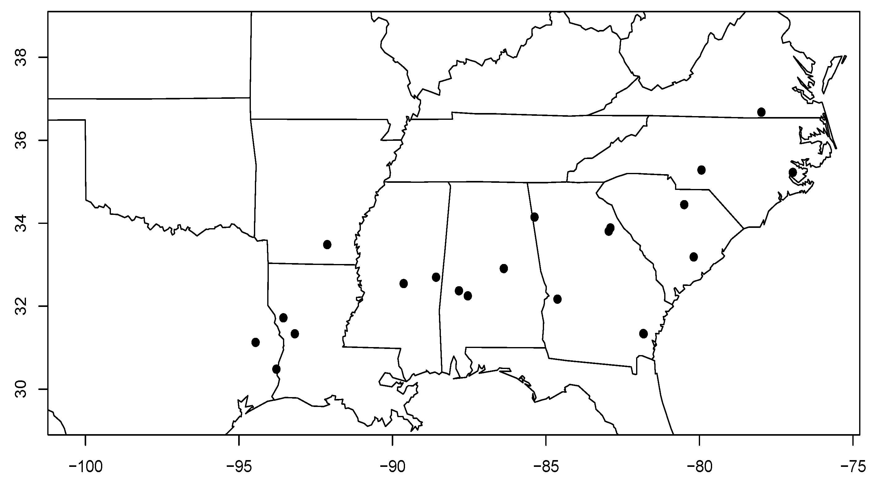
2.1. Study Site Description


| Study Site | State, County | Physiographic Province | Lat. / Long. | Soil Series | Precipitation (mm year ) | Temperature max/min | Density (stems ha) | Plantation Year |
|---|---|---|---|---|---|---|---|---|
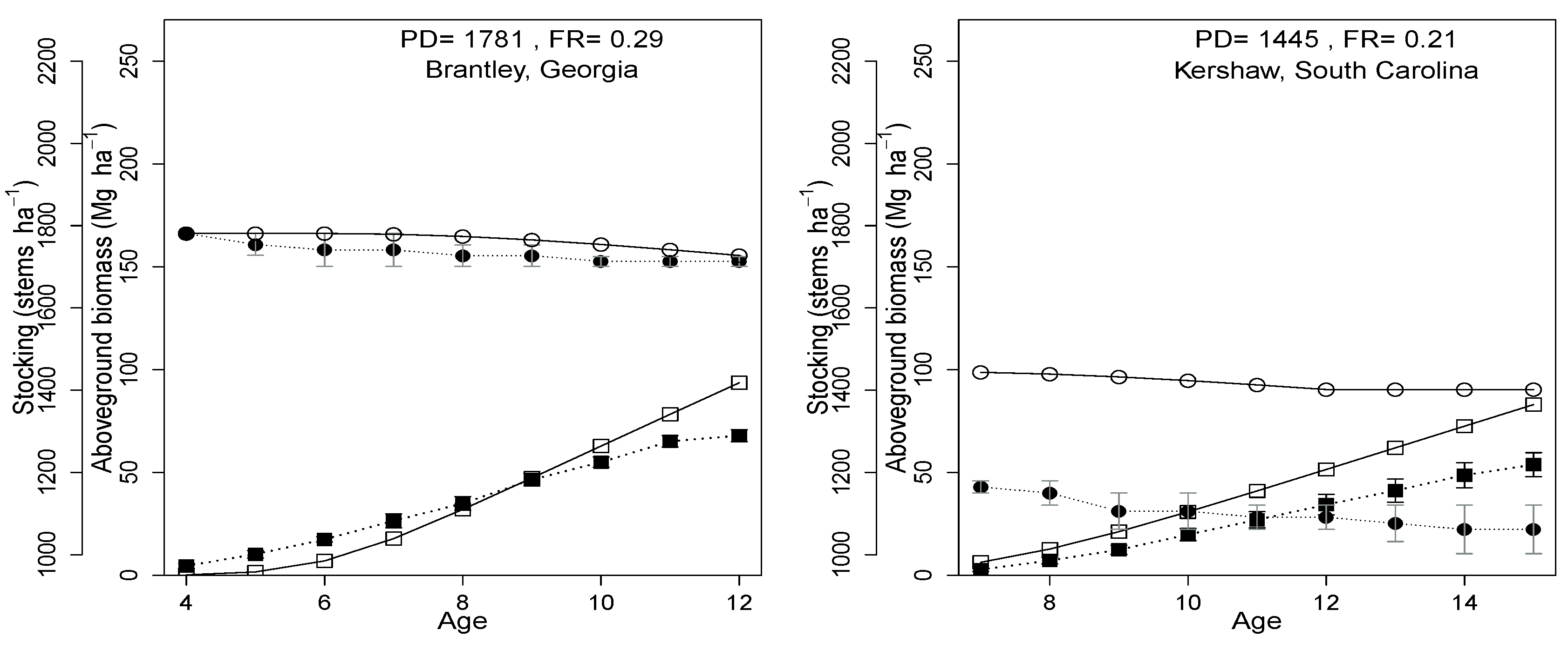
| 180101 | South Carolina, Kershaw | Piedmont | 34.45/-80.50 | Lakeland | 1208.5 | 32.6/-0.5 | 1445 | 1997 |
| 180301 | Georgia, Oglethorpe | Piedmont | 33.89/-82.91 | Mecklenburg | 1237.3 | 32.9/-0.6 | 1640 | 1993 |
| 180601 | Virginia, Brunswick | Piedmont | 36.68/-77.99 | Cecil | 1165.6 | 31.7/-3.0 | 1677 | 1993 |
| 180801 | North Carolina, Craven | LCP | 35.23/-76.97 | Leaf | 1235.9 | 32/0.9 | 1317 | 1992 |
| 181101 | South Carolina, Berkeley | LCP | 33.19/-80.19 | Lynchburg | 1289.5 | 33.4/1.3 | 1622 | 1994 |
| 181201 | Alabama, Coosa | Piedmont | 32.91/-86.38 | Louisa | 1412.6 | 32.6/0.3 | 1457 | 1996 |
| 181502 | Georgia, Floyd | Valley & Ridge | 34.15/-85.38 | Townley | 1371.8 | 32.1/-1.0 | 1655 | 1998 |
| 181503 | Texas, Angelina | WGCP | 31.13/-94.46 | Kurth | 1331.3 | 34.1/2.5 | 1267 | 2000 |
| 182201 | Georgia, Wilkes | Piedmont | 33.81/-82.96 | Appling | 1240.6 | 32.9/-0.3 | 1815 | 1997 |
| 183101 | Louisiana, Sabine | WGCP | 31.72/-93.56 | Sacul | 1370.6 | 33.8/1.2 | 2141 | 1993 |
| 183102 | Louisiana, Vernon | WGCP | 31.34/-93.18 | Sacul | 1489.8 | 33.8/2.1 | 1756 | 1994 |
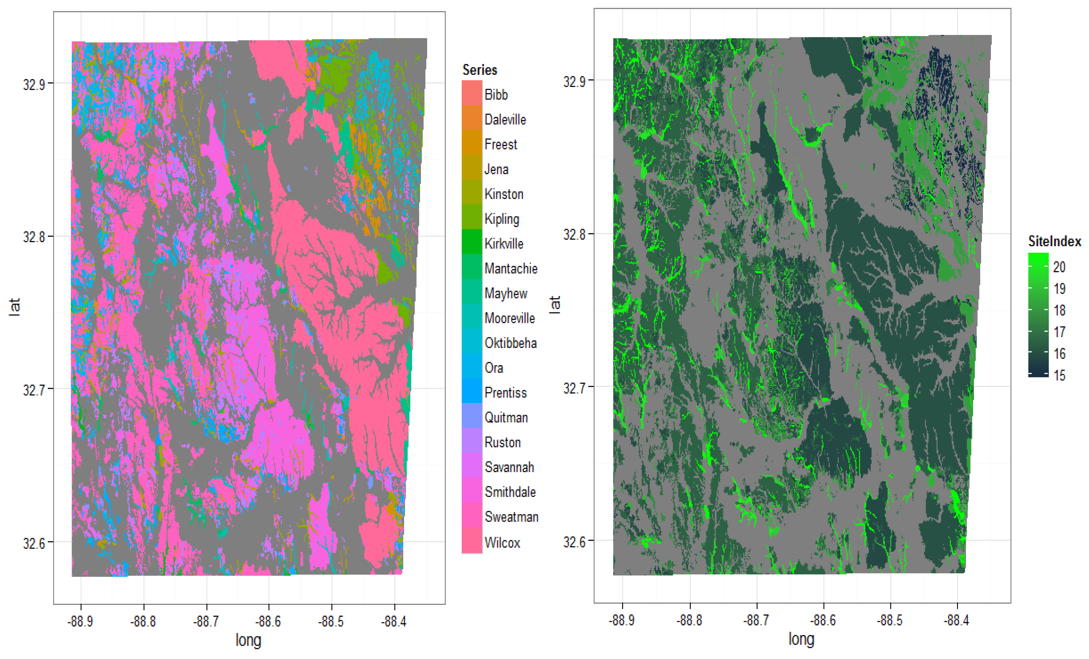
| 183601 | Mississippi, Kemper | EGCP | 32.70/-88.58 | Smithdale | 1451.4 | 33.3/0.6 | 1632 | 1996 |
| 183901 | Alabama, Marengo | EGCP | 32.37/-87.84 | Savannah | 1431.5 | 33.3/1.2 | 1413 | 1998 |
| 184201 | Georgia, Brantley | LCP | 31.34/-81.82 | Leon | 1310.3 | 33.2/4.3 | 1781 | 1994 |
| 184202 | Georgia, Brantley | LCP | 31.34/-81.83 | Leon | 1308.2 | 33.2/4.3 | 1781 | 1995 |
| 184301 | Georgia, Marion | UCP | 32.17/-84.63 | Troup | 1275.9 | 33.1/2.0 | 1862 | 1996 |
| 184401 | Arkansas, Bradley | WGCP | 33.49/-92.13 | Savannah | 1402.1 | 33.5/0.8 | 1247 | 1996 |
| 184501 | Alabama, Marengo | EGCP | 32.25/-87.55 | Brantley | 1418.5 | 33.3/1.4 | 1415 | 1996 |
| 184801 | Texas, Newton | WGCP | 30.48/-93.78 | Evadale | 1496.8 | 33.7/3.7 | 1264 | 1999 |
| 185201 | North Carolina, Montgomery | Piedmont | 35.28/-79.94 | Herndon | 1212.7 | 32.5/-1.0 | 1215 | 1999 |
| 185301 | Mississippi, Montgomery | EGCP | 32.55/ -89.64 | Shubuta | 1491.2 | 33.2 / 0.7 | 1326 | 1997 |
2.2. 3-PG Parameterization
2.3. FR Calculation from Site Index
2.3.1. Calculation of Site Index
2.3.2. Determine Relationship between Stand Volume and Site Index
- Linear (
- Exponential (Volume = e)
- Sigmoid (Volume = )
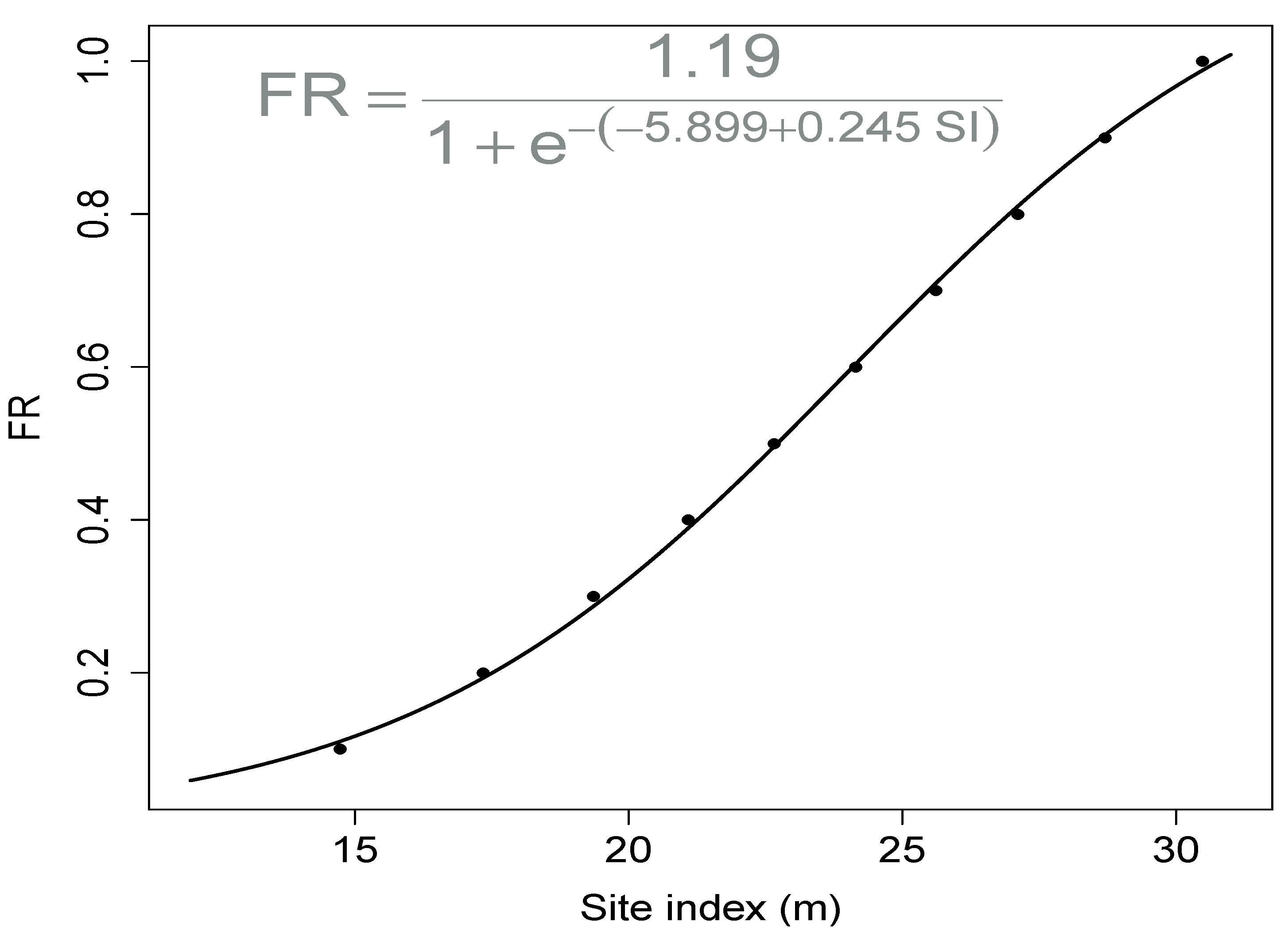
2.3.3. Calculate Relationship between FR and Site Index
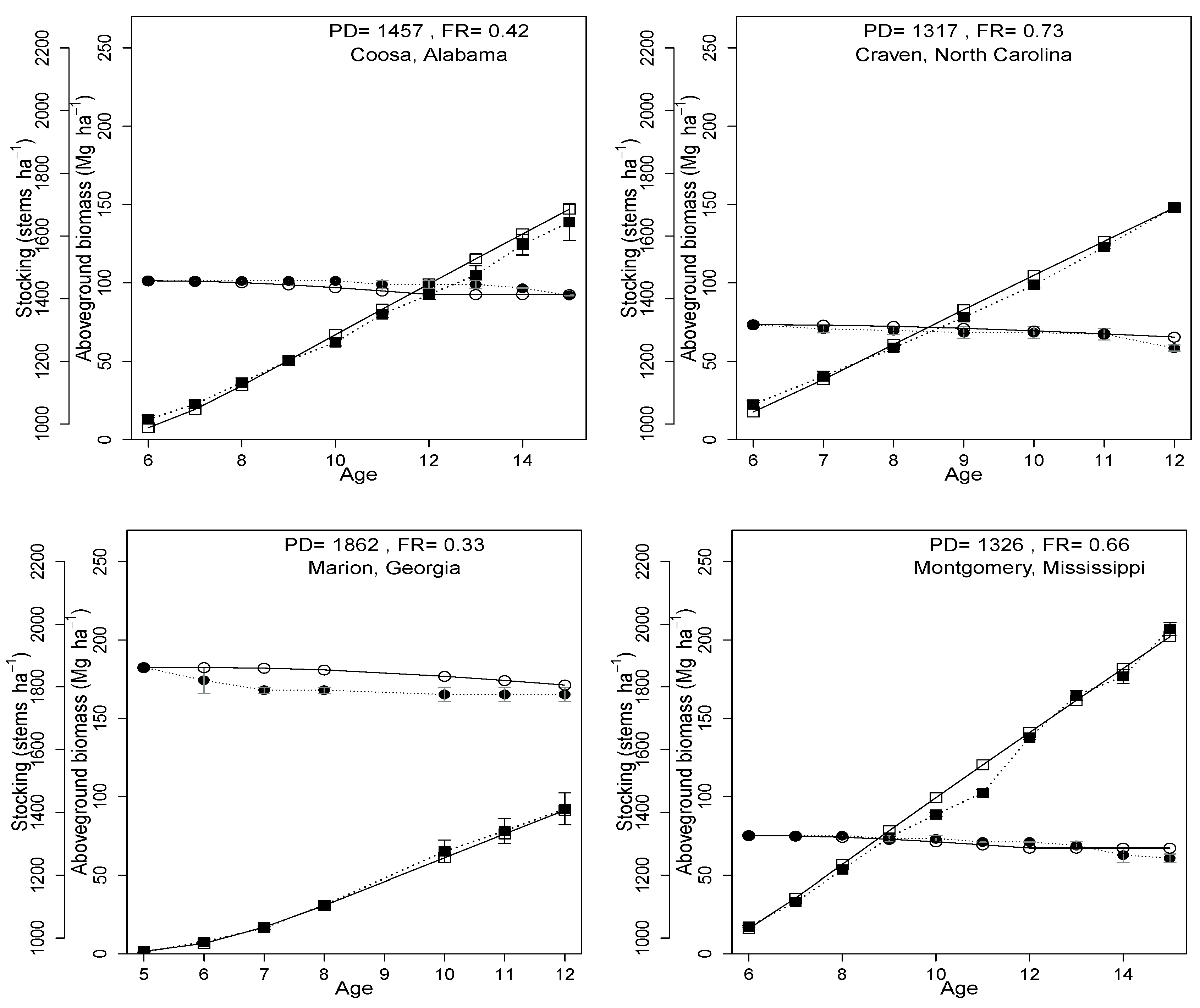
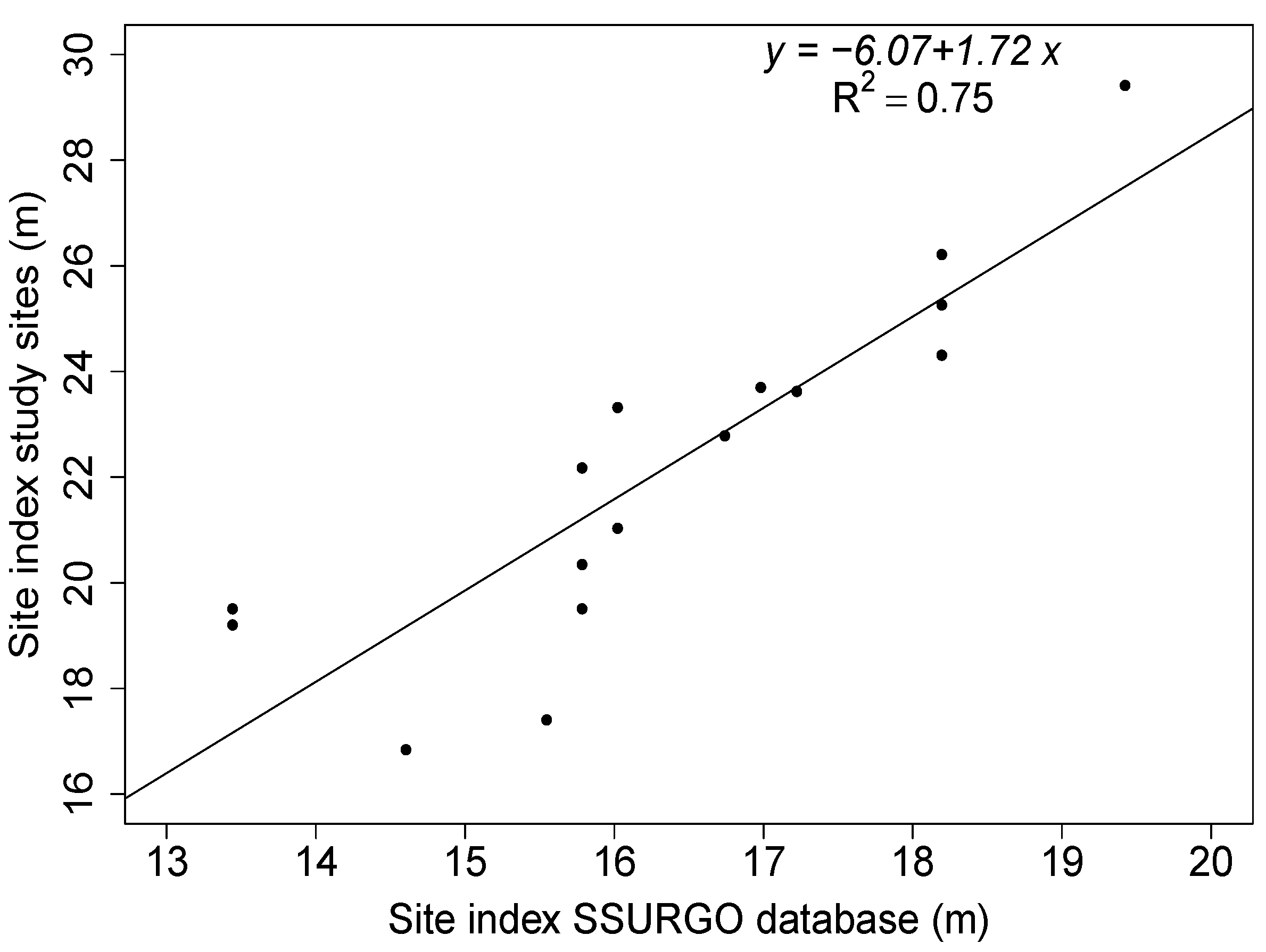
2.4. Validation of the Relationship between FR and Site Index
| Parameters | Meaning | Unit | Value | |
| 1 | pFS2 | Ratio of foliage:stem partitioning at stem diameter = 2 cm | 0.40 | |
| 2 | pFS20 | Ratio of foliage:stem partitioning at stem diameter = 20 cm | 0.25 | |
| 3 | StemConst | Constant in stem mass diameter relationship | 0.10 | |
| 4 | StemPower | Power in stem massvdiameter relationship | 2.50 | |
| 5 | pRx | Maximum fraction of NPP to roots | 0.40 | |
| 6 | pRn | Minimum fraction of NPP to roots | 0.20 | |
| 7 | SLA0 | Projected specific leaf area at the beginning of plantation | m Kg | 6.40 |
| 8 | SLA1 | Projected specific leaf area for mature stand | m Kg | 4.00 |
| 9 | tSLA | Age at which SLA is mean of SLA0 and SLA1 | year | 6.00 |
| 10 | k | Extinction coefficient for APAR by canopy | 0.69 | |
| 11 | fullCanAge | Age at full canopy cover | year | 4.00 |
| 12 | MaxIntcptn | Maximum proportion of rainfall intercepted by canopy | 0.20 | |
| 13 | LAImaxIntcptn | LAI for maximum rainfall interception | 5.00 | |
| 14 | Maximum canopy quantum efficiency | molC molPAR | 0.053 | |
| 15 | MaxCond | Maximum canopy conductance | m s | 0.006 |
| 16 | LAIgcx | Canopy LAI for maximum canopy conductance | 3.00 | |
| 17 | CoeffCond | Defines stomatal response to VPD | mbar | 0.02 |
| 18 | BLcond | Canopy boundary layer conductance | m s | 0.10 |
| 19 | wSx1000 | Maximum stem mass per tree at 1000 trees ha | kg tree | 235.00 |
| 20 | thinPower | Power in self thinning law | 1.60 | |
| 21 | mF | Fraction of mean foliage biomass per tree on dying trees | 0.00 | |
| 22 | mR | Fraction of mean root biomass per tree on dying trees | 0.20 | |
| 23 | mS | Fraction of mean stem biomass per tree on dying trees | 0.40 | |
| 24 | fracBB0 | Branch and bark fraction at stand age 0 | 0.40 | |
| 25 | fracBB1 | Branch and bark fraction for mature stand | 0.10 | |
| 26 | tBB | Age at which brak fraction is mean of fracBB0 and fracBB1 | 15.00 | |
| 27 | gammaFx | Maximum litterfall rate | month | 0.042 |
| 28 | gammaF0 | Litterfall rate at age 0 | month | 0.001 |
| 29 | tgammaF | Age at which litterfall rate is mean of gammaFx and gammaF0 | 18.00 | |
| 30 | Rttover | Average monthly root turnover rate | 0.0168 | |
| 31 | m0 | Value of m when FR is zero | 0.10 | |
| 32 | fN0 | Value of fN when FR is zero | 0.50 | |
| 33 | Tmin | Minimum temperature for growth | C | 4 |
| 34 | Topt | Optimum temperature for growth | C | 25 |
| 35 | Tmax | Maximum temperature for growth | C | 38 |
| 36 | kF | Number of days production lost for each frost day | 1 | |
| 37 | MaxAge | Maximum stand age used to compute relative age | 40 | |
| 38 | nAge | Power of relative age in age modifier | 3 | |
| 39 | rAge | relative age to make age modifier 0.5 | 0.20 | |
| 40 | y | NPP to GPP ratio | 0.47 |
| Location (County, State) | Lat. / Long. | Planting Density (Trees ha) | Age (Years) | FR | Avg max T (C) | Precipitation (mm year) | Soil Series |
|---|---|---|---|---|---|---|---|
| Lancaster, South Carolina | 34.55/-80.63 | 1097 | 12-16 | 0.34 | 36.13 | 1157.60 | Appling |
| Covington, Alabama | 31.20/-86.25 | 1147 | 11-19 | 0.38 | 35.51 | 1547.86 | Florala |
| Kemper, Mississippi | 32.40/-81.44 | 865 | 11-19 | 0.51 | 36.76 | 1429.97 | Wilcox |
| Effingham, Georgia | 36.21/-76.94 | 1509 | 10-20 | 0.35 | 36.28 | 1208.37 | Leefield |
| Bertie, North Carolina | 32.75/-88.45 | 1442 | 10-20 | 0.34 | 33.88 | 1280.63 | Norfolk |
| Howard, Arkansas | 34.03/-94.02 | 1000 | 10-16 | 0.33 | 38.20 | 1375.83 | Sacul |
2.5. Application of FR Model in SSURGO Database
3. Results
3.1. Relationship between Site Index and Volume

| Model Name | Model Form | RMSE | MAE | PRESS |
|---|---|---|---|---|
| Exponential | Volume = e | 20.60 | 15.51 | 13157.4 |
| Sigmoid | Volume = | 19.70 | 16.36 | 12029.6 |
| Linear | Volume = -207.693 + 16.115 SI | 18.51 | 15.33 | 10622.7 |
3.2. Relationship between Site Index and FR
| Volume (m ha) | Site Index (m) | FR |
|---|---|---|
| 26.7 | 10.7 | 0 |
| 52.0 | 14.7 | 0.1 |
| 77.6 | 17.3 | 0.2 |
| 103.0 | 19.4 | 0.3 |
| 128.5 | 21.1 | 0.4 |
| 154.1 | 22.7 | 0.5 |
| 179.7 | 24.2 | 0.6 |
| 205.6 | 25.6 | 0.7 |
| 230.7 | 27.1 | 0.8 |
| 256.2 | 28.7 | 0.9 |
| 281.8 | 30.5 | 1 |

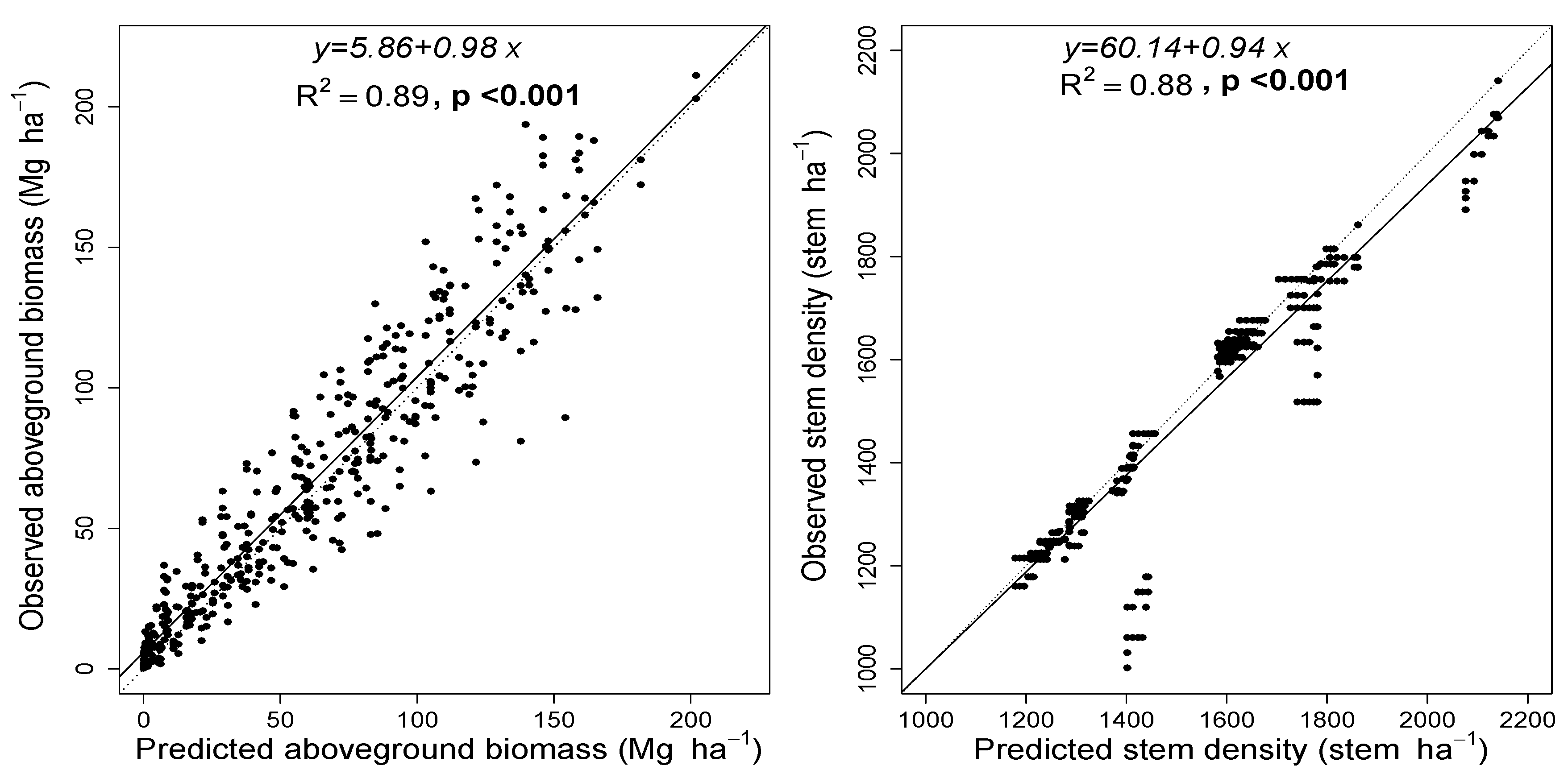
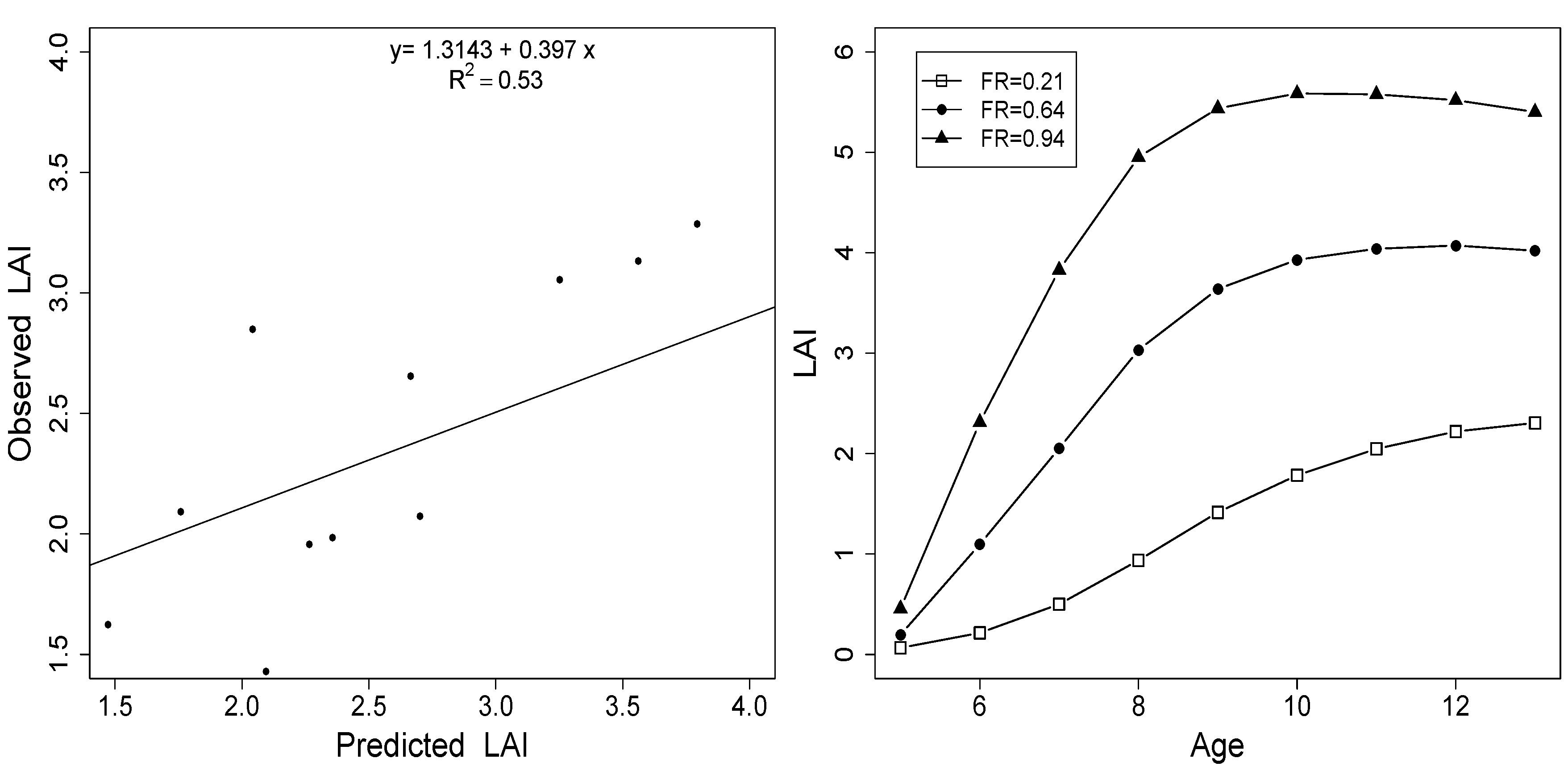
3.3. Model Evaluation


3.4. County Level Productivity Estimation


| Kemper | Brunswick | Brantley | ||||||||||
|---|---|---|---|---|---|---|---|---|---|---|---|---|
| Series | SI | Adjusted SI | FR | Series | SI | Adjusted SI | FR | Series | SI | Adjusted SI | FR | |
| Bibb | 30.5 | 20.7 | 0.36 | Appling | 25.9 | 17.0 | 0.18 | Albany | 29.0 | 19.4 | 0.29 | |
| Daleville | 29.0 | 19.4 | 0.29 | Ashlar | 22.9 | 14.6 | 0.11 | Bladen | 28.7 | 19.2 | 0.28 | |
| Freest | 27.4 | 18.2 | 0.23 | Badin | 24.4 | 15.8 | 0.14 | Bonifay | 25.9 | 16.7 | 0.18 | |
| Jena | 30.5 | 20.7 | 0.36 | Cecil | 25.3 | 16.5 | 0.16 | Centenary | 25.9 | 16.7 | 0.18 | |
| Kinston | 30.5 | 20.7 | 0.36 | Chewacla | 25.6 | 16.7 | 0.17 | Eulonia | 27.4 | 18.2 | 0.23 | |
| Kipling | 27.4 | 18.2 | 0.23 | Emporia | 25.9 | 17.0 | 0.18 | Florala | 27.4 | 18.2 | 0.23 | |
| Kirkville | 29.0 | 19.4 | 0.29 | Enon | 20.4 | 12.8 | 0.07 | Foxworth | 24.4 | 15.8 | 0.14 | |
| Mantachie | 29.9 | 20.2 | 0.33 | Fluvanna | 23.2 | 14.8 | 0.11 | Fuquay | 25.9 | 17.0 | 0.18 | |
| Mayhew | 27.4 | 18.2 | 0.23 | Georgeville | 24.7 | 16.0 | 0.15 | Hurricane | 27.4 | 18.2 | 0.23 | |
| Mooreville | 29.0 | 19.4 | 0.29 | Goldston | 22.6 | 14.4 | 0.10 | Kinston | 30.5 | 20.7 | 0.36 | |
| Oktibbeha | 23.2 | 14.8 | 0.11 | Helena | 25.6 | 16.7 | 0.17 | Lakeland | 22.9 | 14.6 | 0.11 | |
| Ora | 25.3 | 16.5 | 0.16 | Herndon | 24.4 | 15.8 | 0.14 | Leefield | 25.6 | 16.7 | 0.17 | |
| Prentiss | 26.8 | 17.7 | 0.21 | Iredell | 20.4 | 12.8 | 0.07 | Leon | 22.9 | 14.6 | 0.11 | |
| Quitman | 28.0 | 18.7 | 0.25 | Lignum | 23.2 | 14.8 | 0.11 | Lynn Haven | 24.4 | 15.8 | 0.14 | |
| Ruston | 25.6 | 16.7 | 0.17 | Madison | 22.0 | 13.9 | 0.09 | Mascotte | 21.3 | 13.4 | 0.08 | |
| Savannah | 24.7 | 16.0 | 0.15 | Mattaponi | 24.4 | 15.8 | 0.14 | Meggett | 30.5 | 20.7 | 0.36 | |
| Smithdale | 26.2 | 17.2 | 0.19 | Pacolet | 23.8 | 15.3 | 0.12 | Meldrim | 25.9 | 17.0 | 0.18 | |
| Sweatman | 25.3 | 16.5 | 0.16 | Rion | 24.4 | 15.8 | 0.14 | Ogeechee | 27.4 | 18.2 | 0.23 | |
| Wilcox | 24.7 | 16.0 | 0.15 | Riverview | 30.5 | 20.7 | 0.36 | Olustee | 24.4 | 15.8 | 0.14 |
4. Discussion
5. Conclusions
Acknowledgments
Author Contributions
Conflicts of Interest
References
- Landsberg, J.J.; Waring, R.H. A generalized model of forest productivity using simplified concepts of radiation-use efficiency, carbon balance and partitioning. For. Ecol. Manag. 1997, 95, 209–228. [Google Scholar] [CrossRef]
- Almeida, A.C.; Landsberg, J.J.; Sands, P.J. Parameterization of 3-PG model for fast-growing Eucalyptus grandis plantations. For. Ecol. Manag. 2004, 193, 179–195. [Google Scholar] [CrossRef]
- Stape, J.L.; Ryan, M.; Binkley, D. Testing the utility of the 3-PG model for growth of Eucalyptus grandis x urophylla with natural and manipulated supplies of water and nutrients. For. Ecol. Manag. 2004, 193, 219–234. [Google Scholar] [CrossRef]
- Dye, P.J. Modelling growth and water use in four Pinus patula stands with the 3-PG model. South. Afr. For. J. 2001, 191, 53–63. [Google Scholar]
- Landsberg, J.J.; Johnson, K.H.; Albaugh, T.J.; Allen, H.L.; McKeand, S.E. Applying 3-PG, a simple process-based model designed to produce practical results, to data from loblolly pine experiments. For. Sci. 2001, 47, 43–51. [Google Scholar]
- Bryars, C.; Maier, C.; Zhao, D.; Kane, M.; Borders, B.; Will, R.; Teskey, R. Fixed physiological parameters in the 3-PG model produced accurate estimates of loblolly pine growth on sites in different geographic regions. For. Ecol. Manag. 2013, 289, 501–514. [Google Scholar] [CrossRef]
- Rodŕiguez, R.; Espinosa, M.; Real, P.; Inzunza, J. Analysis of productivity of radiata pine plantations under different silvicultural regimes using the 3-PG process-based model. Aust. For. J. 2002, 65, 165–172. [Google Scholar] [CrossRef]
- Gonzalez-Benecke, C.A.; Jokela, E.J.; Cropper, W.P., Jr.; Bracho, R.; Ledu, D.J. Parameterization of the 3-PG model for Pinus elliottii stands using alternative methods to estimate fertility rating, biomass partitioning and canopy closure. For. Ecol. Manag. 2014, 327, 55–75. [Google Scholar] [CrossRef]
- Coops, N.C.; Waring, R.H.; Law, B.E. Assessing the past and future distribution and productivity of ponderosa pine in the Pacific Northwest using a process model, 3-PG. Ecol. Model. 2005, 183, 107–124. [Google Scholar] [CrossRef]
- Landsberg, J.; Waring, R.; Coops, N. Performance of the forest productivity model 3-PG applied to a wide range of forest types. For. Ecol. Manag. 2003, 172, 199–214. [Google Scholar] [CrossRef]
- Landsberg, J.; Sands, P. Chapter 9-The 3-PG Process-Based Model. In Physiological Ecology of Forest Production; Terrestrial Ecology; Elsevier: Amsterdam, The Netherlands, 2011; Volume 4, pp. 241–282. [Google Scholar]
- Sampson, D.A.; Wynne, R.H.; Seiler, J.R. Edaphic and climatic effects on forest stand development, net primary production, and net ecosystem productivity simulated for Coastal Plain loblolly pine in Virginia. J. Geophys. Res. 2008, 113, 1–14. [Google Scholar] [CrossRef]
- Vega-Nieva, D.J.; Tomé, M.; Tomé, J.; Fontes, L.; Soares, P.; Ortiz, L.; Basurco, F.; Rodríguez-Soalleiro, R. Developing a general method for the estimation of fertility rating parameter of the 3-PG model: Application in Eucalyptus globulus plantations in Northwestern Spain. Can. J. For. Res. 2013, 43, 627–636. [Google Scholar] [CrossRef]
- Pérez-Cruzado, C.; Muñoz Sáez, F.; Basurco, F.; Riesco, G.; Rodŕiguez-Soalleiro, R. Combining empirical models and the process-based model 3-PG to predict Eucalyptus nitens plantations growth in Spain. For. Ecol. Manag. 2011, 262, 1067–1077. [Google Scholar] [CrossRef]
- Burkhart, H.E.; Tomé, M. Modeling Forest Trees and Stands; Springer: Amsterdam, The Netherlands, 2012; p. 457. [Google Scholar]
- Dye, P.J.; Jacobs, S.; Drew, D. Verification of 3-PG growth and water-use predictions in twelve Eucalyptus plantation stands in Zululand, South Africa. For. Ecol. Manag. 2004, 193, 197–218. [Google Scholar] [CrossRef]
- USDA-NRCS (U.S. Department of Agriculture-Natural Resources Conservation Service). Available online: http://www.nrcs.usda.gov/wps/portal/nrcs/detail/soils/survey/geo/?cid=nrcs142p2_053627 (accessed on 13 June 2015).
- Fox, T.R.; Allen, H.L.; Albaugh, T.J.; Rubilar, R.; Carlson, C.A. Tree nutrition and forest fertilization of pine plantations in the southern United States. South. J. Appl. For. 2007, 31, 5–11. [Google Scholar]
- Allen, H.L. Forest fertilizers: Nutrient amendment, stand productivity, and environmental impact. J. For. 1987, 85, 37–46. [Google Scholar]
- Allen, H.L.; Dougherty, P.M.; Campbell, R.G. Manipulation of water and nutrients — practice and opportunity in southern U.S. pine forests. For. Ecol. Manag. 1990, 30, 437–453. [Google Scholar] [CrossRef]
- Sampson, A.; Allen, H.L. Regional influences of soil available water and climate, and leaf area index on simulated loblolly pine productivity. For. Ecol. Manag. 1999, 124, 1–12. [Google Scholar] [CrossRef]
- Jokela, E.J.; Martin, T.A. Effects of ontogeny and soil nutrient supply on production, allocation, and leaf area efficiency in loblolly and slash pine stands. Can. J. For. Res. 2000, 30, 1511–1524. [Google Scholar] [CrossRef]
- Will, R.E.; Munger, G.T.; Zhang, Y.; Borders, B.E. Effects of annual fertilization and complete competition control on current annual increment, foliar development, and growth efficiency of different aged Pinus taeda stands. Can. J. For. Res. 2002, 32, 1728–1740. [Google Scholar] [CrossRef]
- Carlson, C.A.; Fox, T.R.; Allen, H.L.; Albaugh, T.J. Modeling mid-rotation fertilizer response using the age-shift approach. For. Ecol. Manag. 2008, 256, 256–262. [Google Scholar] [CrossRef]
- Lu, J.; Sun, G.; McNulty, S.G.; Amatya, D.M. Modeling actual evapotranspiration from forested waterwater across the southeastern United States. J. Am. Wat. Res. Assoc. 2003, 39, 887–896. [Google Scholar] [CrossRef]
- Albaugh, T.J.; Allen, H.L.; Dougherty, P.M.; Kress, L.W.; King, J.S. Leaf area and above- and belowground growth responses of loblolly pine to nutrient and water additions. For. Sci. 1998, 44, 317–328. [Google Scholar]
- Samuelson, L.J.; Marrianne, F.G.; Stokes, T.A.; Coleman, M.D. Fertilizaton not irrigation influences hydralulic traits in plantation-grown loblolly pine. For. Ecol. Manag. 2008, 255, 3331–3339. [Google Scholar] [CrossRef]
- Cobb, W.R.; Will, R.E.; Daniels, R.F.; Jacobson, M.A. Aboveground biomass and nitrogen in four short-rotation woody crop species growing with different water and nutrient availabilities. For. Ecol. Manag. 2008, 12, 4032–4039. [Google Scholar] [CrossRef]
- Will, R.; Fox, T.; Akers, M.; Domec, J.C.; Gonzalez-Benecke, C.; Jokela, E.; Kane, M.; Laviner, M.; Lokuta, G.; Markewitz, D.; et al. A range-wide experiment to investigate nutrient and soil moisture interactions in loblolly pine plantations. Forests 2015, 6, 2014–2028. [Google Scholar] [CrossRef]
- FNC. Eight Year Growth and Foliar Response of Young Loblolly Pine Planations to Repeated Nutrient Additions; Bulletin 62, Forest Productivity Cooperative, North Carolina State Univeristy, Virginia Tech and Universidad de Concepciòn: Raleigh, NC, USA, 2008. [Google Scholar]
- Akers, M.K.; Kane, M.; Zhao, D.; Teskey, R.O.; Daniels, R.F. Effects of planting density and cultural intensity on stand and crown attributes of mid-rotation loblolly pine plantations. For. Ecol. Manag. 2013, 310, 468–475. [Google Scholar] [CrossRef]
- Sampson, D.A.; Amatya, D.M.; Lawson, C.D.B.; Skagg, R.W. Leaf area index (LAI) of loblolly pine and emergent vegetaion following a harvest. Trans. Am. Soc. Agr. Biol. Eng. 2011, 54, 2057–2066. [Google Scholar]
- Dalla-Tea, F.; Jokela, E.J. Needlefall, canopy light interception, and productivity of young intensively managed slash and loblolly pine stands. For. Sci. 1991, 37, 1298–1313. [Google Scholar]
- Will, R.E.; Barron, G.A.; Burkes, E.C.; Shiver, B.; Teskey, R.O. Relationship between intercept radiation, net photosynthesis, respiration, and rate of stem volume growth of Pinus taeda and Pinus elliottii stands of different densities. For. Ecol. Manag. 2001, 154, 155–163. [Google Scholar] [CrossRef]
- Colbert, S.R.; Jokela, E.J.; Neary, D.G. Effects of annual fertilization and sustained weed control on dry matter partitioning, leaf area, and growth efficiency of juvenile loblolly and slash pine. For. Sci. 1990, 36, 995–1014. [Google Scholar]
- McCrady, R.L.; Jokela, E.J. Growth phenology and crown structure of selected loblolly pine families planted at two spacings. For. Sci. 1995, 42, 46–57. [Google Scholar]
- Sampson, D.A.; Allen, H.L. Light attenuation in a 14-year-old loblolly pine stand as influenced by fertilization and irrigation. Trees 1998, 13, 80–87. [Google Scholar] [CrossRef]
- Isaac, M.E.; Kimaro, A.A. Diagnosis of nutrient imbalances with vector analysis in agroforestry systems. J. Environ. Qual. 2011, 40, 860–866. [Google Scholar] [CrossRef] [PubMed]
- Westermann, D.T. Fertility Managemen. In Potato Health Management; ISBN 0-89054-144-2. Rowe, R.C., Ed.; APS Press: St. Paul, MN, USA, 1993; Chapter 9; pp. 77–86. [Google Scholar]
- Salifu, K.F.; Timmer, V.R. Optimizing nitrogen loading of Picea mariana seedlings during nursery culture. Can. J. For. Res. 2003, 33, 1287–1294. [Google Scholar] [CrossRef]
- Diéguez-Aranda, U.; Burkhart, H.E.; Amateis, R.L. Dynamic site model for loblolly pine (Pinus taeda L.) plantations in the United States. For. Sci. 2005, 52, 262–272. [Google Scholar]
- Cieszewski, C.J.; Bailey, R.L. Generalized algebraic difference approach: Theory based deviation on dynamic site equations with polymorphism and variable asymptotes. For. Sci. 2000, 46, 116–126. [Google Scholar]
- Gyawali, N.; Burkhart, H.E. General response functions to silvicultural treatments in loblolly pine plantations. Can. J. For. Res. 2015, 45, 252–265. [Google Scholar] [CrossRef]
- Van Deusen, P.C.; Sullivan, A.D.; Matvey, T.G. A prediction system for cubic foot volume of loblolly pine applicable through much of its range. South. J. Appl. For. 1981, 5, 186–189. [Google Scholar]
- Schulz, R.P. Loblolly Pine: The Ecology and Culture of Loblolly Pine (Pinus Taeda L.); USDA: Washington, DC, USA, 1997; Volume 713. [Google Scholar]
- Cao, Q.V.; Baldwin, V.C.; Lohrey, R.E. Site index curves for direct-seeded loblolly and longleaf pines in Louisiana. South. J. Appl. For. 1997, 21, 134–138. [Google Scholar]
- Harrison, M.; Kane, M. PMRC Coastal Plain Culture/density Study: Age 12 Analysis; Technical Report; Plantation Management Research Cooperative, Daniel B. Warnell School of Forest Resources, University of Georgia: Athens, GA, USA, 2008. [Google Scholar]
- Gonzalez-Benecke, C.; Gezan, S.; Albaugh, T.; Allen, H.; Burkhart, H.; Fox, T.; Jokela, E.; Maier, C.; Martin, T.; Rubilar, R.; et al. Local and general above-stump biomass functions for loblolly pine and slash pine trees. For. Ecol. Manag. 2014, 334, 254–276. [Google Scholar] [CrossRef]
- Piñeiro, G.; Perlman, S.; Guerschman, J.P.; Parule, J.M. How to evaluate models: Observed vs. predicted or predicted vs. observed. Ecol. Model. 2008, 216, 316–322. [Google Scholar] [CrossRef]
- Loague, K.; Green, R.E. Statistical and graphical methods for evaluating solute transport models: Overview and application. J. Contam. Hydrol. 1991, 7, 51–73. [Google Scholar] [CrossRef]
- Amateis, R.L.; Liu, J.; Ducey, M.J.; Allen, H.L. Modeling response to midrotation nitrogen and phosphorus fertilization in loblolly pine plantations. South. J. Appl. For. 2000, 24, 207–221. [Google Scholar]
- Skovsgaard, J.P.; Vanclay, J.K. Forest site productivity: A review of the evolution of the dendrometric concepts for even-aged stands. Forestry 2008, 81, 13–31. [Google Scholar] [CrossRef]
- Sands, P.J.; Landsberg, J.J. Parameterization of 3-PG for planation grown Eucalyptus globulus. For. Ecol. Manag. 2002, 163, 273–292. [Google Scholar] [CrossRef]
- Pinjuv, G.; Mason, E.G.; Watt, M. Quantitative validation and comparison of a range of forest growth model types. For. Ecol. Manag. 2006, 236, 37–46. [Google Scholar] [CrossRef]
- Tickle, P.K.; Coops, N.C.; Hafner, S.D.; Team, T.B.S. Assessing forest productivity at local scales across a native eucalypt forest using a process model, 3PG-SPATIAL. For. Ecol. Manag. 2001, 152, 275–291. [Google Scholar] [CrossRef]
- Vose, J.M.; Dougherty, P.M.; Long, J.N.; Smith, F.W.; Gholz, H.L.; Curran, P.J. Factors infuencing the amount and distribution of leaf area of pine stands. Ecol. Bull. 1994, 43, 102–114. [Google Scholar]
- Zhao, D.; Kane, M.; Borders, B.; Subedi, S.; Akers, M. Effects of cultural intensity and planting density on stand-level aboveground biomass production and allocation for 12-year-old loblolly pine plantations in the Upper Coastal Plain and Piedmont of the southeastern United States. Can. J. For. Res. 2012, 42, 111–122. [Google Scholar] [CrossRef]
- Peduzzi, A.; Wynne, R.H.; Fox, T.R.; Nelson, R.F.; Thomas, V.A. Estimating leaf area index in intensively managed pine plantations using airborne laser scanner data. For. Ecol. Manag. 2012, 270, 54–65. [Google Scholar] [CrossRef]
- Vose, M.; Allen, H.L. Leaf area, stemwood growth, and nutrition relationships in loblolly pine. For. Sci. 1988, 34, 547–563. [Google Scholar]
- Romell, L. Man-made nature of northern lands. In Proceedings and Papers of the Sixth Technical Meeting of The International Union for Conservation of Nature and Natural Resources; Society for the Promotion of Nature Reserves, London: Edinburgh, UK, 1957; pp. 51–53. [Google Scholar]
- Tamm, C.O. Determination of nutrient requirements of forest stands. Int. Rev. For. Res. 1964, 1, 115–170. [Google Scholar]
- Miller, H.G. Forest fertilization: Some guiding concepts. Forestry 1981, 54, 157–167. [Google Scholar] [CrossRef]
- Piatek, K.B.; Allen, H.L. Are forest floors in mid-rotation stands of loblolly pine (Pinus taeda) a sink for nitrogen and phosphorus? Can. J. For. Res 2001, 31, 1164–1174. [Google Scholar] [CrossRef]
- Kiser, L.C.; Fox, T.R. Soil accumulation of nitrogen and phosphorus following annual fertilization of loblolly pine and sweetgum on sandy sites. Soil Sci. Soc. Am. J. 2012, 76, 2278–2288. [Google Scholar] [CrossRef]
- Albaugh, T.J.; Allen, H.L.; Fox, T.R. Individual tree crown and stand development in Pinus taeda under different fertilization and irrigation regimes. For. Ecol. Manag. 2006, 234, 10–23. [Google Scholar] [CrossRef]
- Borders, B.; Bailey, R.L. Loblolly pine – pushing the limits of growth. South. J. Appl. For. 2001, 25, 69–74. [Google Scholar]
- Haywood, J.D.; Burton, J.D. Phosphorous fertilizer, soils, and site preparation influence loblolly pine productivity. New For. 1990, 3, 275–287. [Google Scholar] [CrossRef]
© 2015 by the authors; licensee MDPI, Basel, Switzerland. This article is an open access article distributed under the terms and conditions of the Creative Commons Attribution license (http://creativecommons.org/licenses/by/4.0/).
Share and Cite
Subedi, S.; Fox, T.R.; Wynne, R.H. Determination of Fertility Rating (FR) in the 3-PG Model for Loblolly Pine Plantations in the Southeastern United States Based on Site Index. Forests 2015, 6, 3002-3027. https://doi.org/10.3390/f6093002
Subedi S, Fox TR, Wynne RH. Determination of Fertility Rating (FR) in the 3-PG Model for Loblolly Pine Plantations in the Southeastern United States Based on Site Index. Forests. 2015; 6(9):3002-3027. https://doi.org/10.3390/f6093002
Chicago/Turabian StyleSubedi, Santosh, Thomas R. Fox, and Randolph H. Wynne. 2015. "Determination of Fertility Rating (FR) in the 3-PG Model for Loblolly Pine Plantations in the Southeastern United States Based on Site Index" Forests 6, no. 9: 3002-3027. https://doi.org/10.3390/f6093002