Unmanned Aerial System and Machine Learning Techniques Help to Detect Dead Woody Components in a Tropical Dry Forest


1
Laboratorio de Investigación e Innovación Tecnológica (LIIT), Universidad Estatal a Distancia (UNED), San José 474-2050, Costa Rica
2
Alberta Centre for Earth Observation Sciences, Department of Earth and Atmospheric Sciences, University of Alberta, Edmonton, AB T6G 2E3, Canada
3
Department of Geography, Ludwig Maximilian University, Luisenstrasse 37, 80333 Munich, Bavaria, Germany
*
Author to whom correspondence should be addressed.
Forests 2020, 11(8), 827; https://doi.org/10.3390/f11080827
Submission received: 22 June 2020
/
Revised: 21 July 2020
/
Accepted: 28 July 2020
/
Published: 29 July 2020
(This article belongs to the Special Issue Forestry Applications of Unmanned Aerial Vehicles (UAVs) 2020)
Abstract
:Background and Objectives: Increased frequency and intensity of drought events are predicted to occur throughout the world because of climate change. These extreme climate events result in higher tree mortality and fraction of dead woody components, phenomena that are currently being reported worldwide as critical indicators of the impacts of climate change on forest diversity and function. In this paper, we assess the accuracy and processing times of ten machine learning (ML) techniques, applied to multispectral unmanned aerial vehicle (UAV) data to detect dead canopy woody components. Materials and Methods: This work was conducted on five secondary dry forest plots located at the Santa Rosa National Park Environmental Monitoring Super Site, Costa Rica. Results: The coverage of dead woody components at the selected secondary dry forest plots was estimated to range from 4.8% to 16.1%, with no differences between the successional stages. Of the ten ML techniques, the support vector machine with radial kernel (SVMR) and random forests (RF) provided the highest accuracies (0.982 vs. 0.98, respectively). Of these two ML algorithms, the processing time of SVMR was longer than the processing time of RF (8735.64 s vs. 989 s). Conclusions: Our results demonstrate that it is feasible to detect and quantify dead woody components, such as dead stands and fallen trees, using a combination of high-resolution UAV data and ML algorithms. Using this technology, accuracy values higher than 95% were achieved. However, it is important to account for a series of factors, such as the optimization of the tuning parameters of the ML algorithms, the environmental conditions and the time of the UAV data acquisition.
1. Introduction
Increasing emissions of greenhouse gases are acknowledged by the scientific community to result in a significant increase in the global mean temperature [1]. In some regions, this is likely to increase the frequency and severity of droughts and heatwaves [2,3]. Resulting from these extreme weather phenomena, long-term field studies are reporting tree growth decline and mortality [4,5,6,7]. Anomalously long or intense mortality events can have long-term impacts on a range of ecosystems and populations [8]. Mortality can impact biodiversity functions and ecosystem services such as carbon and nutrient cycling, which could exacerbate biophysical and biochemical climate feedbacks [8]. One potential consequence of such mortality events is the increased growth of understory vegetation, which in turn can impact successional pathways, productivity and surface hydrology [5]. Therefore, increasing tree mortality can reduce competition among plant communities, leading to a reduction in the ability of forests to absorb CO2 [6].
Tree mortality can take place through different mechanisms. For instance, hydraulic failure occurs when water supply is reduced during high evaporative demand, causing xylem conduits to become air-filled. This halts the flow of water, bringing plant tissues to complete cellular death [5,9]. Another mechanism, carbon starvation, occurs when plant stomata close to prevent hydraulic failure, reducing carbon uptake at a time of continued metabolic demand for carbohydrates [5]. Carbon starvation may be exacerbated during drought by photoinhibition and increased respiratory demands associated with elevated temperatures [10]. Hydraulic failure occurs if a drought is sufficiently intense for plants to run out of water before they run out of carbon [11]. In tropical forests, mortality is driven by a combination of hydraulic failure and carbon starvation processes: where mortality is most likely triggered by hydraulic processes, their effects can be aggravated by rapid limitations in carbon uptake [9].
In the last decade, machine learning (ML) has become a favored tool of remote sensing studies, as a set of computational algorithms and techniques that acquire knowledge from existing data based on inference strategies [12,13,14]. The principle of these algorithms is to model complex classes and accept a variety of input data without making assumptions about the underlying statistical distribution of a given dataset [12]. In remote sensing, a number of studies have found that ML methods tend to produce higher accuracy than traditional parametric classifiers [12,15,16,17]. Among ML algorithms, other approaches such as artificial neural networks (ANN), deep learning (DL), decision trees (DT), boosting machines (BM) and support vector machines (SVM) can be found.
ANN and DL algorithms can map features to classes by associating elements in one set of data with elements in a second set, motivated by the assumption that the human brain and artificial intelligence apply similar decision criteria to classification tasks [18]. DL is similar to ANN but uses deeper neural networks using various hierarchical representations [19]. DT is among the most intuitive simple classifiers due to its flexibility, intuitive simplicity and computational efficiency [13]. Random forest (RF) is a specific DT classification model that produces multiple subsets of training samples and variables that are randomly selected [20]. In RF, the same sample can be selected several times, while others may not be selected at all [21]. Likewise, BM models are DTs that incorporate a process known as “boosting”: this algorithm generates an ensemble of decision trees, where each successive tree is fitted with the remaining residuals from the previous trees [12]. Finally, SVM is very popular in remote sensing because of its ability to classify highly dimensional data with a limited number of training samples [22].
Unmanned aerial vehicles (UAVs) are well suited to addressing current issues in the remote sensing of tropical forest ecology and conservation [23]. Compared with manned aircrafts, UAVs are more flexible and economically affordable, which enables data acquisition of plant canopy measurements at optimal weather conditions [23]. In tropical regions, UAV-derived information has been used in a wide range of ecological applications. For instance, in neotropical dry forests, UAV derived information has been applied to conservation biology [24], the detection of liana infested regions [25], ecological monitoring [26], latent heat flux [27] and canopy temperature of liana-infested and non-liana infested areas [28].
Given the emerging importance of quantifying tree mortality as a metric of the impacts of climate change in tropical forests, we explore the use of UAVs and ten machine learning models to detect and quantify dead woody components at a tropical dry forest (TDF) site. We conducted this study in five forest plots that cover a gradient of secondary TDFs, in order to evaluate the role of ecosystem succession on the extent of tree mortality.
2. Materials and Methods
2.1. Study Site
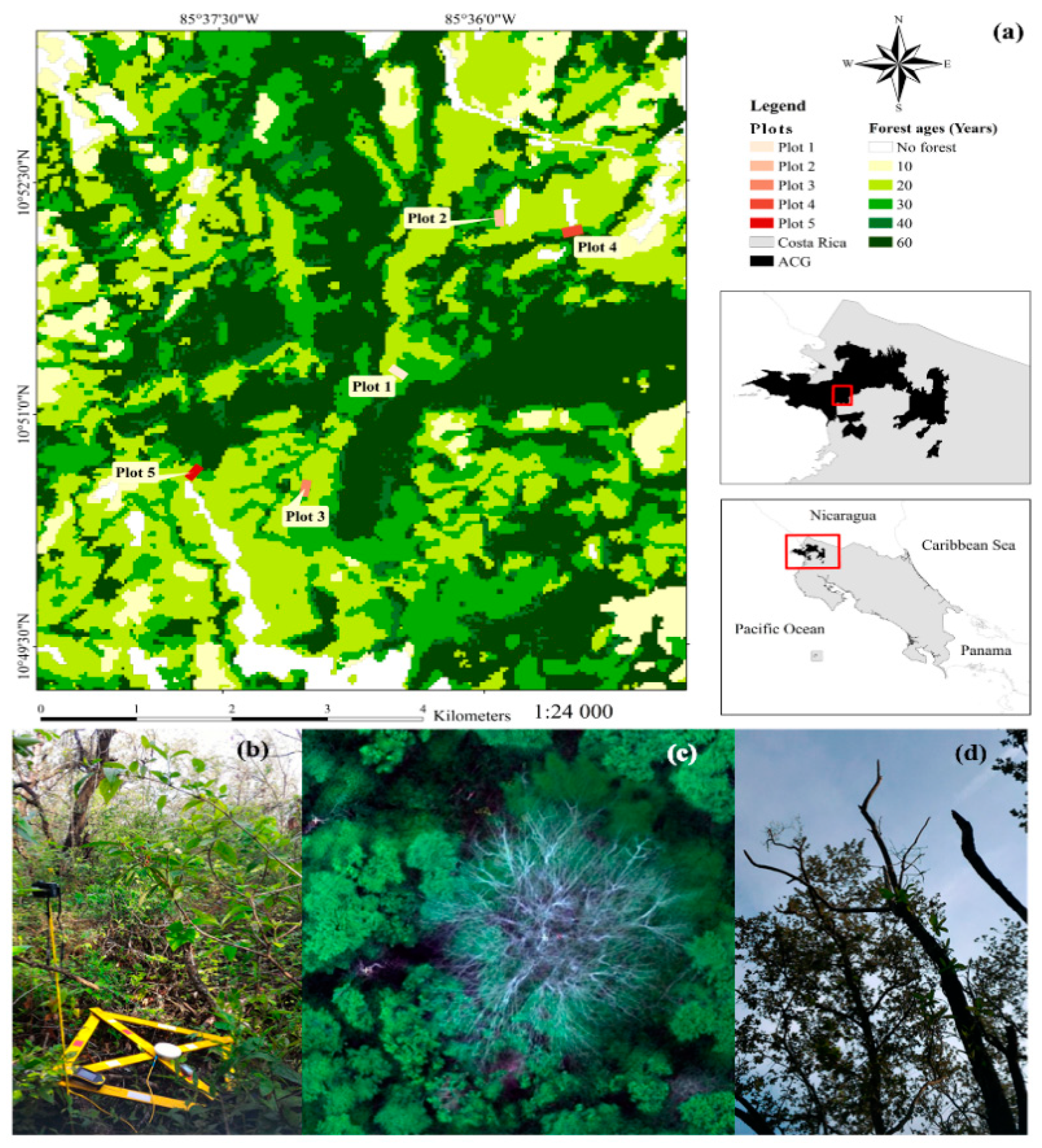
We conducted this study at the Santa Rosa National Park Environmental Monitoring Super Site (SR-EMSS), Guanacaste, Costa Rica (Figure 1). The SRNP-EMSS has a mosaic of TDFs in various ecological successional stages that once suffered from intense deforestation [15]. The mean temperature is 25 °C and the average annual rainfall is 1750 mm [29]. The dry season lasts for a minimum of 5–6 months, and it usually extends from approximately late December to mid-May [29].
In this study, a gradient of the SR-EMSS was sampled following the findings of Li et al. [25] (Table 1). In this area, succession is divided into early, intermediate and late forests based on age since abandonment [30]. At the SRNP-EMSS, early forests are composed of patches of woody vegetation, which include several species of shrubs, small trees and young trees with a maximum height of approximately 6–8 m. Trees at the early stages of TDFs lose nearly all their leaves during the dry season [31]. Early forest stages are dominated by species well adapted to open habitats, such as Cochlospermum vitifolium, Gliricidia sepium and Rehdera trinervis, as well as sun-loving species (heliophytes) that have anemochory and autochory dispersal syndromes [32]. The intermediate and late successional stages show significant differences in structure and composition [33]. These differences are generally driven by species turnover, which causes a very dynamic structure and forest species composition [34]. The intermediate and late successional stages have two vegetation layers. The first layer encompasses fast-growing deciduous tree species that reach a maximum height of 10–15 m. The second layer is below the canopy and is composed of lianas (woody vines) and adults of more shade-tolerant evergreen species and juveniles of many species [32,33]. Dominant species in the early stage are Rehdera trinervis and Guazuma ulmifolia, whereas Calycophyllum candidissimum and Hymenaea courbaril are dominant in the late stage [33]. Not all trees on the intermediate and late stage are deciduous: several evergreen species are present.
2.2. Field Acquisition
Field work was conducted in five 200 × 100 m plots, listed in Table 1, from May to July 2017. In the field, observations were made on the following categories: (1) dead components, (2) living components and (3) understory. The dead components category comprises the following: (1.1) dead woody components, (1.2) dead stand trees, (1.3) dead fallen trees, (1.4) non-photosynthetic woody components within the tree crown and (1.5) dead woody components of lianas (woody vines). The living components category comprises the following: (2.1) healthy canopy trees and (2.2) healthy lianas within the tree crowns. The understory category includes the following: (3.1) understory vegetation (shrubs, small trees and young trees), (3.2) canopy gaps (grass-like vegetation, vines, shrubs and small trees), (3.3) exposed rocks and soils and (3.4) shadowed vegetation.
On each plot, the locations of 50 dead components, 50 living components and 50 understory components were recorded. This was achieved by systematically surveying each plot with transects every 25 m along the short side of the plot. A compass and a Trimble® GeoXT® 6000 differential GPS (average precision of 0.5 m horizontal and 0.54 m vertical; Trimble, Sunnyvale, CA, USA) with a Hurricane antenna were used to record the locations. These components are referred to as ground control points (GCPs) from herein.
A RedEdgeTM 3 (MicaSense, Seattle, WA, USA) multispectral camera onboard a Draganflyer XP-4 (DraganFly Inc., Saskatoon, Canada), operating at 120 m height from the ground, was used to collect images at all plots. The Draganflyer XP-4 is a quadcopter equipped with a three-axes electronic gimbal. The airframe was equipped with a three-axes gyrostabilizer, magnetometer and accelerometer. The RedEdgeTM 3 camera has five lenses with a focal length of 5.5 mm, lens field of view of 47.2° and 1280 × 960 pixels. Each lens provides a separate 16-bit GeoTIFF image centered on a specific wavelength and full width at half maximum (FWHM): blue at 475 nm (FWHM: 20 nm), green at 560 nm (FWHM 20 nm), red at 668 nm (FWHM: 10 nm), red edge at 717 nm (FWHM: 10 nm) and near-infrared at 840 nm (FWHM: 40 nm).
Spectral signatures and multispectral images of three reference panels (a white Spectralon panel, a grey RedEdgeTM 3 panel and flat black presentation cardboard) were collected prior to and after each flight to perform a radiometric calibration to surface reflectance. Specifically, at each site, 20 RedEdgeTM 3 images were acquired at a 1.5 m distance from the reference materials. Moreover, 20 spectra were acquired of every reference material, at a 0.75 m distance from the panel. These spectra were acquired with a UniSpec-SC Dual Channel Spectrometer (PP Systems, Amesbury, MA, USA) that has a wavelength range of 310–1100 nm, FWHM of <10 nm and a sampling of 3.3 nm. The instrument’s dark signal noise removal was performed by taking a dark scan in the beginning of the measurements and later, after every ten sampled measurements. Similarly, the integration time was adjusted with the fiber-optic exposed to a white reference panel, also done in the beginning and after every ten samples. The spectra were acquired by averaging 10 scans.
2.3. Data Preprocessing
The UAV image preprocessing workflow involved three steps: (1) radiometric calibration, (2) mosaicking, and (3) data reduction and transformation.
2.3.1. Radiometric Correction and Mosaicking
To radiometrically correct the RedEdgeTM 3 UAV images, an empirical line method was used, as suggested by Kalacska et al. [35] and Smith and Milton [36]. The generation of orthomosaics was performed by the Pix4Dmapper (Pix4D Pro, Lausanne, Switzerland, version v3.3.29). However, in this program, the radiometric correction step was skipped because it was previously performed with the empirical line method. Five single band mosaics were obtained, one mosaic per each RedEdgeTM band. The mosaics were then orthorectified using 7 to 10 GCPs distributed across each plot and described in Section 2.2.
2.3.2. Data Reduction and Transformation
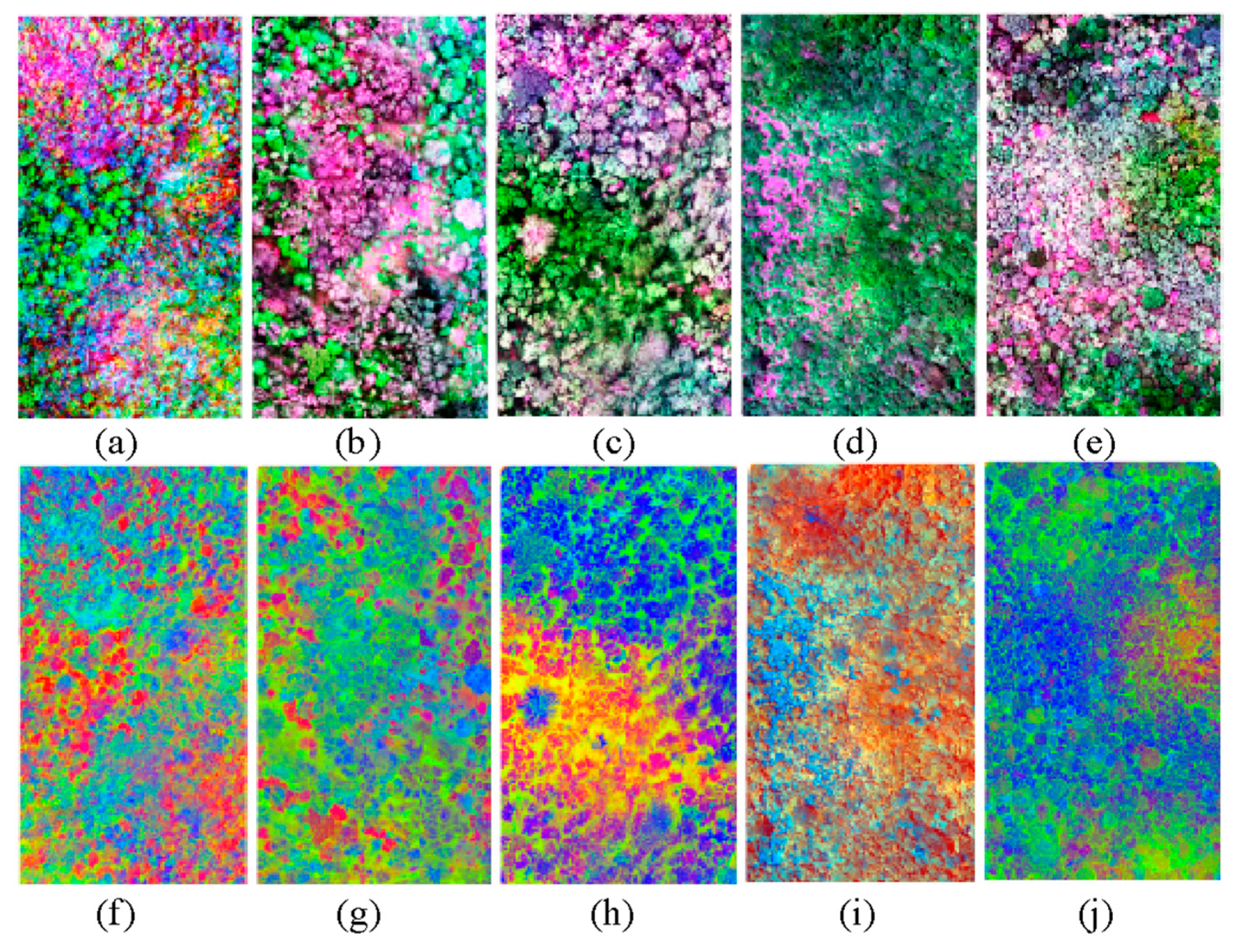
Despite multispectral sensors having advantages over Red Green Blue (RGB) technology due to their larger number of bands and thus larger amount of information, their use implies a substantial increase in data volume. Image transformation of high-resolution remote sensing data has been proven to be useful for the quantification of forest structure and biomass [37] and in the estimation of the extension and succession of tropical dry forests [15], among other applications. In this study, three transformation methods were applied to reduce redundancies in individual bands in order to bring out the total information captured by a combination of bands: principal components analysis (PCA), tasseled cap (TC) and texture analysis (TA) (Figure 2). All transformations were performed using the five multispectral mosaics. In the case of the PCA transformation, the first principal components were retained, but in the case of the TC transformation, only the third component was retained. The TA transformation was conducted using a Gabor filter, restricted to a maximum of five scales and ten directions, to search for elements in a localized region of an image with specific frequency content in particular directions [38].
2.4. Classification Models
The “No Free Lunch” theorem of computing sciences states that, without having substantive information about the modeling problem, there is no single model that is better than other models [39]. In this context, Kuhn and Johnson [17] suggested trying a wide variety of classification models to determine which model performs better. Consequently, this study used ten ML classification algorithms, shown in Table 2: support vector machines with linear kernel (SVML), support vector machines with polynomial kernel (SVMP), support vector machines with radial kernel (SVMR), random forest (RF), conditional inference tree (CIT), C4.5-like trees (C45), gradient boosting machines (GBM), neural network (NNT), averaged neural network (ANN) and deep neural network (DNET). This approach covers most of the available classification models of support vector machines, decision trees, boosting machines and artificial neural networks.
2.5. Creation of Training and Validation Datasets
The total number of 2250 pixels of the multispectral mosaics (450 pixels per mosaic, five mosaics in total) was divided into two datasets: training and validation. The training dataset was used for the model development and the validation dataset was used to estimate the performance of the model. This was achieved in three steps. In the first step, a 3 × 3-pixel area was extracted from the multispectral mosaics around each of the 750 ground truth observations (dead components, living components, understory). This step was conducted using the raster extraction function of the QGIS software package (QGIS Development Team, 2009, QGIS Geographic Information System, Open Source Geospatial Foundation, v3.8). In the case of leafless crowns of the dead component’s category, care was taken to select pixels from the central regions of crowns to ensure that dead woody components, as opposed to understory, would dominate the collected spectra. In the third step, this dataset was randomly split into a training dataset (70% of the pixels) and a validation dataset (30% of the pixels) using the “createDataPartition” function of the R program.
2.6. Implementation of Classification Models
The optimal number of training samples was estimated using the bootstrap “632 method” of the “Caret” package of the R program. This was done to avoid overfitting the classification models: the “632 method” creates a performance estimate that is a combination of a simple bootstrap estimate and an estimate from re-predicting the training set [40]. Bootstrap error rates tend to have less uncertainty than other methods such as k-fold cross-validation, especially if the training set size is small [17]. Likewise, the optimal tune-up parameters of the classification models were estimated with the “expand.grid:caret” and “tuneGrid:caret” functions of the R program using several combinations of values and parameters, shown in Table 2. Two kinds of classification models were generated to quantify the extent of mortality across the five TDF successional plots: five plot-specific models and a general model. The plot-specific models were trained only with data from one plot. The general model was trained and validated with data from the five plots. This is in accordance with the findings of Miltiadou et al. [41], who found that a model that is based on all possible training samples and patterns can perform better than a model generated from a single sampled plot with a lesser number of samples.
2.7. Model Validation
The models were validated by calculating the accuracy and kappa statistics. These statistics were calculated on a per-pixel basis rather than per crown or trunk because the classification was performed using pixels and not objects. Specifically, these metrics were estimated using the validation dataset, with the function “confusionMatrix:caret” of the R program.
2.8. Differences in the Spatial Coverage of the Dead Woody Components between Plots
The spatial coverage of each of the three categories (dead components, living components and understory) of the study was investigated by transforming the multispectral (raster) image mosaics into a vector format. This work was carried out using the conversion function of the QGIS software package. Finally, potential statistical differences between the means of these three categories were studied using the one-way analysis of variance (ANOVA) and Tukey’s post hoc tests.
3. Results
3.1. Effect of Tuning Parameters on the Accuracy Values
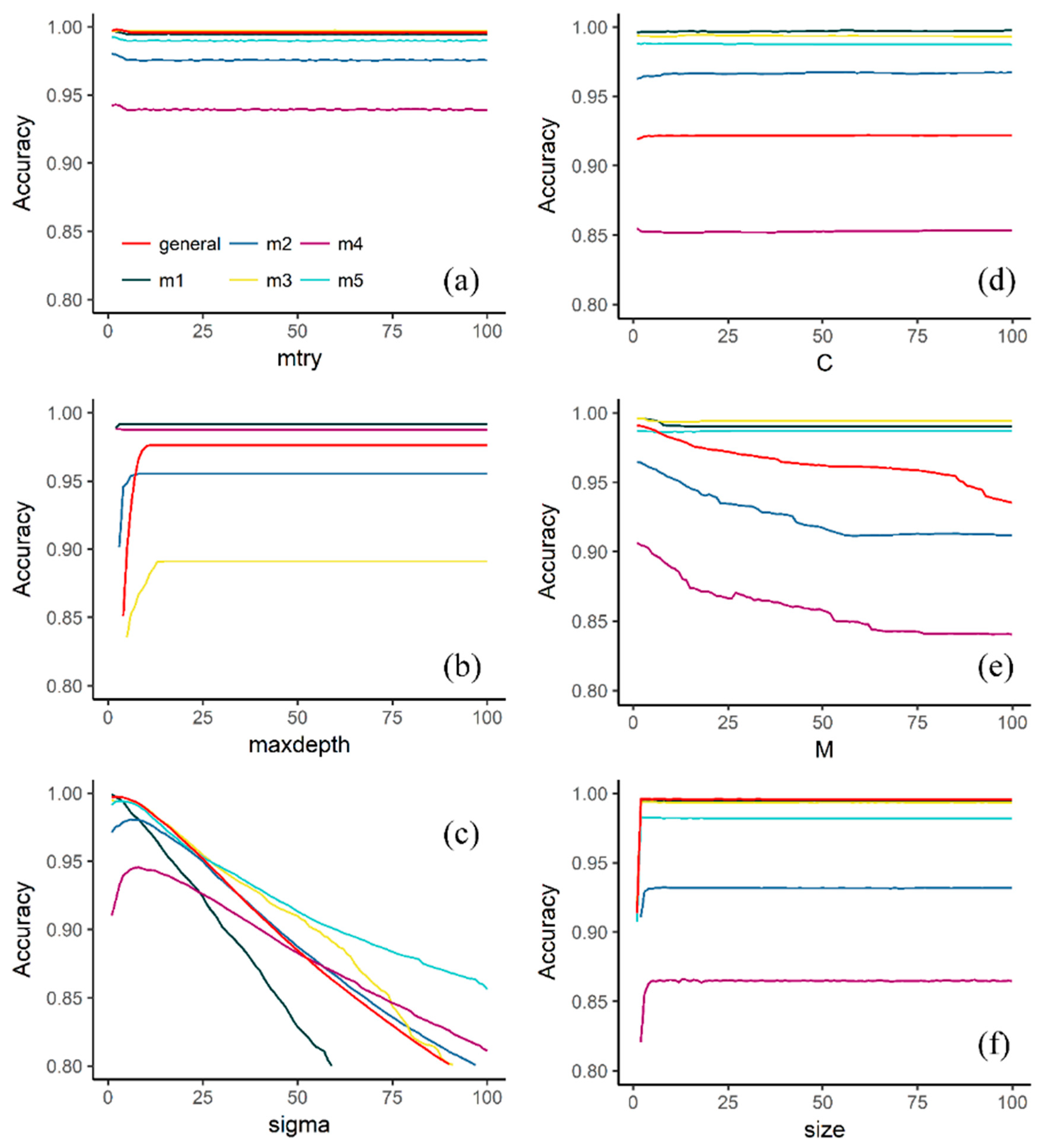
Regarding the tuning parameters used in the study, the results indicate that the models display a varied selection of available parameters. For instance, CIT, C45T, RF, SVML and SVMR (Figure 3) required a maximum of two tuning parameters, whereas SVMP, GBM, ANNT and DNET required three or more tuning parameters and even more complex parametrization, such as applying learning rates, in the case of GBM and DNET. Although ANNT and GBM required a more complex implementation than the other models, they performed similarly in terms of accuracy.
Looking at the tuning parameters of the models, the results suggest that some models were more sensitive than others. Figure 4 shows that RF, CIT, SVML, NNET, ANNT and SVMP remain stable after the values of the driver parameters increase. On the contrary, the accuracy of SVMR and C45T decreases as the value of the driver parameters increases (Figure 3). Models such as RF, CIT, SVML and NNET exhibited a kind of asymptote on the accuracy values when certain tuning parameter values were reached (Figure 3). The latter suggests that at a certain point, no matter whether the numbers of the input parameters grew, the accuracy remained stable. Contrary to this, models such as SVMR and C45T reached their maximum accuracy values at some point and then their accuracy decreased as the values of the driver parameters increased (Figure 3).
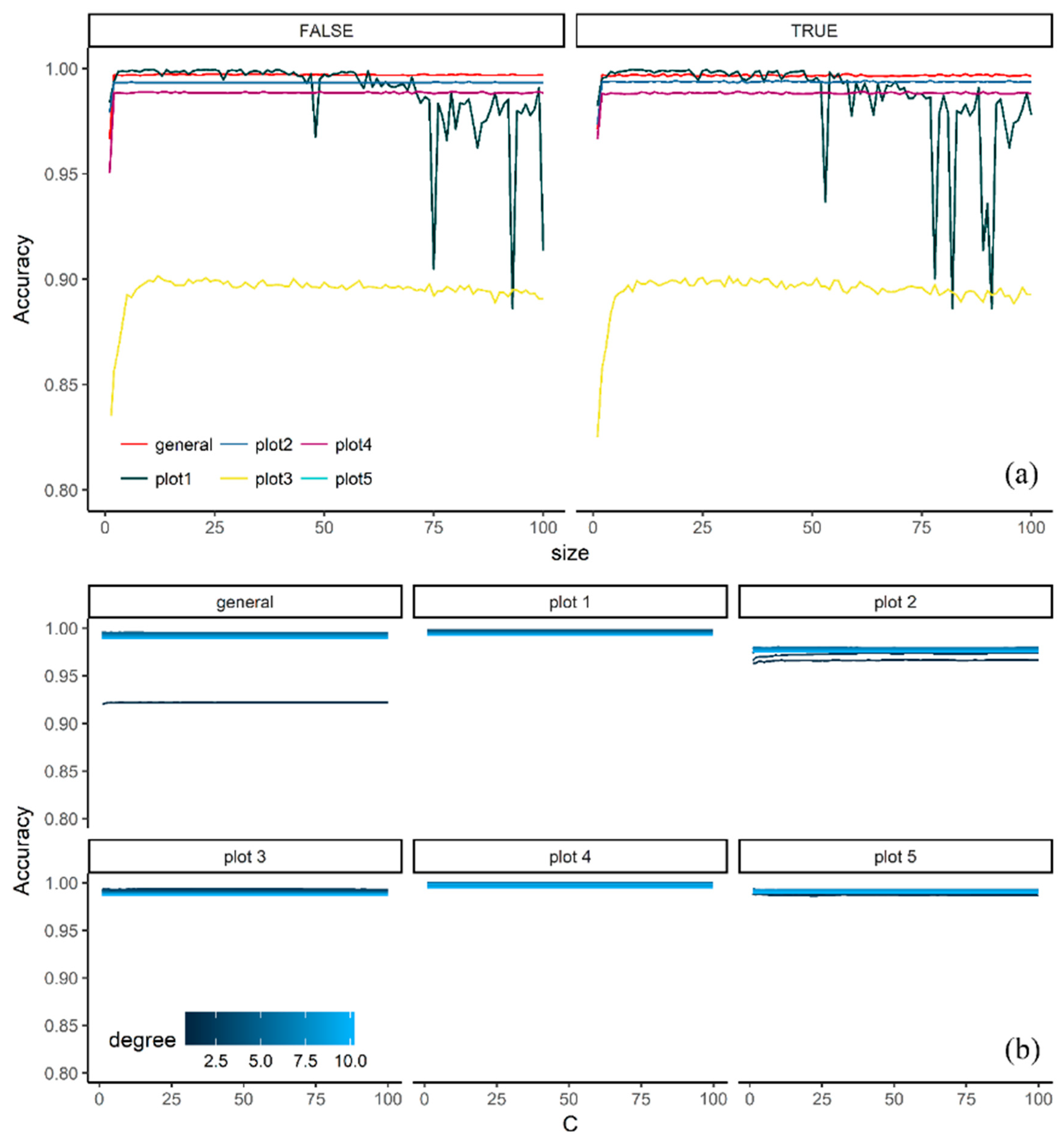
Even though models such ANNT (Figure 4a) and GBM required a more complex implementation than the other models (Table 3), their performance was not always superior to the other models in all plots. For instance, in CIT (Figure 3b) and ANNT (Figure 4a), plot #3 showed lower accuracies than the other plots. Similarly, RF, SVML, NNET and ANNT showed a similar pattern on plot #4. However, in the case of ANNT, the general model displayed an accuracy drop, suggesting that the accuracy was somehow influenced by the bagging operation (Figure 4).
3.2. Model Selection
Of the ten ML models, RF and SVMR reported the highest accuracy values in the classification of dead woody components across the five secondary TDF plots, whereas the lowest accuracy values were reported by CIT, DNET and SVML (Table 3). The SVMR had the highest accuracy value with 0.982, followed by RF with 0.980 and GBM with 0.977.
As shown in Table 3, the processing times vary between the models. The SVMR reported the highest processing time (4690 s), followed by GBM (2839 s) and RF (1523 s). It should be noted that the relatively high standard deviations of the models (e.g., SVMR: 8735 s) suggest variation between the different implementations. The neural networks algorithms (ANNT, NNET and DNET) were the most time-consuming models. The ANNT was the most time-consuming model (69,307.8 sec), followed by NNET (9271.3 sec) and SVMP (8188.3 sec). The most efficient models in terms of processing times were CIT (173.9 sec), C45T (373.8 sec) and SVML (595.6 sec), respectively. Consequently, RF was chosen to run the final classification since it had the highest accuracy and the lowest processing time.
The repeated measures ANOVA shows that the processing times and accuracy of the models were significantly different at a 95% confidence level, but this was not the case for the kappa values (Table 4). Specifically, with 95% of confidence, the accuracy (mean = 4.67, F-value = 150, sign = 0.000) and time (mean = 0.886, F-value = 0.886, sign = 0.004) values from the ML models showed significant differences.
The results of the analysis of the Tukey test indicate that there are two accuracy groups: the first is constituted by the ANNT, CIT, C45T, NNET, RF, SVMP and SVMR algorithms and the second group is composed of the GBM, DNET and SVML algorithms (Table 5). In terms of ML family models, neural networks and support vector machines belong to both accuracy groups, while decision tree models are exclusive to the first group. The gradient boosting machines and deep learning models are exclusive of the second group.
Regarding time, the post hoc test indicates that, at the accuracy level, there are three groups: the first is constituted by CIT, C45T, RF and SVML algorithms; the second by DNET, GBM, NNET, SVMP and SVMR algorithms, and the third group by the ANNT algorithm.
3.3. Extent of Dead Woody Components
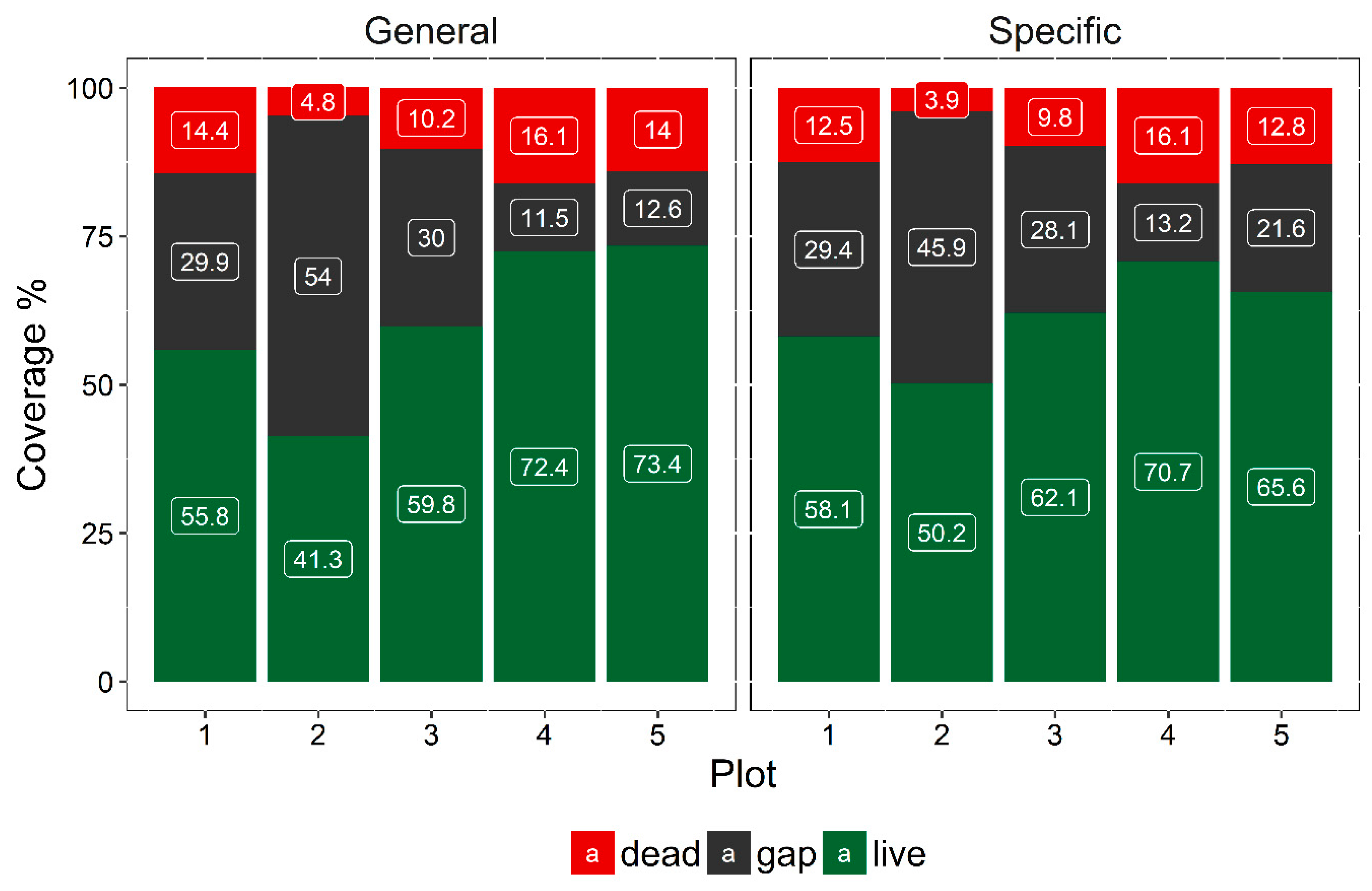
The coverage of the dead woody components ranges from 4.8% to 16.1% for the general model and from 3.9% to 16.1% for the specific model, as shown in Figure 5. The average coverage is 11.9% for the generic model and 11.0% for the specific model. As such, the estimate that the general model gives for the spatial extent of dead components is slightly higher than the estimate given by the specific model.
The results of the analysis of variance of the coverage of dead woody components at the five plots indicated that there are significant differences in the coverage of dead woody components at the five plots (Table 6).
The results of the analysis of the Tukey test indicate that there are three different groups regarding dead woody components (Table 7). The first group is constituted by plots #1 (intermediate-intermediate), #4 (early-early) and #5 (intermediate-intermediate); the second group by plot #3 (intermediate-intermediate), and the third group by plot #2 (early-intermediate).
The highest coverage of the dead components is reported in plot #4, #5 and #1, while the lowest coverage of the dead components is reported in plot #2, a secondary early-intermediate forest patch, followed by plot #3, a secondary intermediate-intermediate forest patch with a high liana infestation. Comparing the general and specific models, both models report similar values for these plots, contrary to plots #1 and #5, where the estimates deviate the most (Figure 6).
4. Discussion
4.1. Effect of Tuning Parameters on the Accuracy Values and Performance of Selected Models
This paper examined the performance of ten ML algorithms on the classification of dead woody components using UAV-based imagery. Our results show that the accuracy of the ML classifiers, as expected for algorithm fitting exercises, is affected by the chosen tuning parameters. With the optimal tuning parameters, the best three classification models reported accuracy values higher than 0.97 whereas, with the least optimal tuning parameters, the accuracy values were close to 0.8. This outcome conforms to the argument by Castelvecchi [42], who suggested that ML models should not be used as a black box, but instead, parametrization should be carefully considered.
All ML models provided high classification accuracy values for the detection of dead, living and understory components. However, the accuracy values of the RF, SVMP and GBM were higher than those of the other models. These models also had relatively low processing times. As such, our results conform to those by Li et al. [25], Meddens et al. [43] and Garrity et al. [44].
4.2. Extension of Dead Woody Components
This study demonstrates that it is possible to detect and quantify dead woody components in a secondary TDF across the successional gradient. The spatial extent of the dead woody components ranges from 4.8% to 16.1% in the five forest plots, with an overall accuracy of 98% and a kappa value of 0.958.
We found that the highest coverage of the dead components was present in the secondary early-early forest, represented by plot #4. However, plot #4 is in a very early successional stage, with a sparse canopy and abundant canopy gaps which increase the spatial coverage for understory. In early successional stages, the Jaragua grass is also abundant, which, together with the shadowing issues, could cause an overestimation of dead woody components. This is because, on one hand, the Jaragua could mimic the response of dead vegetation, and on the other hand, some dead woody components could be masked by the shadows. Consequently, the low accuracy value of plot #4 could be explained by the shadowed components and the abundance of Jarajua grass.
The intermediate-intermediate stages (plots #1 and #5) also show high coverage of the dead components (14.4% and 14%, respectively) that is not statistically different to the early-early successional stage (plot #4). Therefore, our results are in accordance with the findings of Cao et al. [34], who found that the intermediate successional stage of a TDF has a higher growth rate and relatively low mortality rates. On the other hand, the early-intermediate stages, represented by plot #2, show the lowest coverage of the dead components (4.8%).The differences in coverage of dead woody components between successional stages could be explained by the susceptibility of specific trees to mortality mechanisms such as hydraulic failure and carbon starvation.
4.3. Dead Woody Components and Their Ecological Implications
In a TDF, droughts and liana infestation are factors that drive the path of succession [31], which in turn influences the extent of dead woody components. The consequences of drought on forest function and structure depend on which trees are the most adversely affected [4,45]. For instance, Bennett [46] found that, in larger trees, droughts had a more detrimental impact on the growth and mortality rates. In forests, large trees play keystone ecological roles by creating unique micro-environments for nesting cavities [32]. Furthermore, large trees account for a more significant proportion of ecosystem-level transpiration than smaller trees, and their drought-related decline could create detrimental canopy transpiration contributions to cloud formation [47].
In neotropical forests, liana coverage is increasing as a result of higher CO2 concentration, increased disturbance and decreased precipitation [48,49,50]. In TDFs, lianas can be abundant and play a more important role in forest dynamics and mortality than in other tropical ecosystems [50]. Since lianas reduce growth and survival of their host trees [51], with less investment in supporting tissues than in the case of other kinds of growth forms, they can significantly contribute to tree mortality rates [52]. For instance, Li et al. [25] found a significant impact of liana infestation on tree mortality in an intermediate secondary forest at the same study area as ours (same area as plot #1).
4.4. The Influence of Enviromental Conditions and Time in Accuracy of Remotely Sensed Data at Tropical Dry Forests
Irrespective of the performance and tuning parameters of the ML algorithms used, the accuracy of the remotely sensed data is also influenced by environmental conditions and the time of data acquisition. The time of the year and the time of the day play crucial roles in the quality of the remotely sensed data [53,54]. In TDF, the time of the year is associated with the seasonality of the vegetation [55]. For instance, in the study area, most of the trees lose nearly all their leaves during the dry season; therefore, without field work, it is difficult to differentiate a seasonal leafless tree from a dead tree or a tree with dead woody components. On the other hand, the time of the day unequivocally determines the coverage of shadows within the canopy. Due to the lower solar angles, the solar energy is spread over a larger surface, increasing the coverage of shadows [53]. Consequently, it could be expected that, by restricting the UAV flights to noon, the issues associated with shadows would be solved. However, in this study, the shadowing issues were mitigated by flying at noon but not solved.
5. Conclusions
This study demonstrates that it is feasible to detect and quantify dead woody components such as dead stands and fallen trees using multispectral UAV imagery and ML techniques. Of the ML algorithms used in the study, the relatively high accuracy values and low processing times of RF and SVMP made them superior to the other models. Likewise, this study illustrates, on one hand, how the tuning parameters of the ML algorithms affect the accuracy of the classification results, and, on the other hand, how a maximum number of training samples can increase the accuracy of ML classification models.
This study found differences in the coverage of dead woody components across the successional stages of a secondary tropical dry forest. The early successional stages showed the highest coverage of dead woody components, followed by the intermediate stage. Although we found differences between plots, there were no differences in dead woody components between the early and intermediate successional stages.
Finally, further research related to this study could include discrimination of each dead woody component—for instance, the identification of individual dead trees, which could be used for carbon and nutrient cycle modeling.
Author Contributions
Conceptualization, C.C.-V. and A.S.-A.; methodology, C.C.-V. and A.S.-A.; software, C.C.-V.; validation, C.C.-V.; formal analysis, C.C.-V.; investigation, C.C.-V.; resources, A.S.-A.; data curation, C.C.-V.; writing—original draft preparation, C.C.-V. and A.S.-A.; writing—review and editing, C.C.-V., A.S.-A., K.L. and P.M.; visualization, C.C.-V.; supervision, A.S.-A.; project administration, A.S.-A.; funding acquisition, C.C.-V. and A.S.-A. All authors have read and agreed to the published version of the manuscript.
Funding
This work was carried out with the aid of a grant from the Inter-American Institute for Global Change Research (IAI) Collaborative Research Network (CRN3-025), the National Science and Engineering Research Council of Canada (NSERC) and the support from the Universidad Estatal a Distancia (UNED) through the Acuerdo de Mejoramiento Institucional (AMI).
Acknowledgments
We thank Jose Antonio Guzman for previous discussions about the experimental design and his valuable comments and recommendations regarding early versions of this manuscript. We acknowledge the support of the Guanacaste Conservation Area and the Costa Rica Tropi-Dry staff. We thank all students and field assistants that help during the field work.
Conflicts of Interest
The authors declare no conflict of interest. The founding sponsors had no role in the design of the study; in the collection, analyses, or interpretation of data; in the writing of the manuscript, and in the decision to publish the results.
References
- Masson-Delmotte, V.; Zhai, P.; Pörtner, H.-O.; Roberts, D.; Skea, J.; Calvo, E.; Priyadarshi, B.; Shukla, R.; Ferrat, M.; Haughey, E.; et al. Climate Change and Land: An IPCC Special Report on Climate Change, Desertification, Land Degradation, Sustainable Land Management, Food Security, and Greenhouse Gas Fluxes in Terrestrial Ecosystems; IPCC: Geneva, Switzerland, 2019. [Google Scholar]
- Seager, R.; Ting, M.; Held, I.; Kushnir, Y.; Lu, J.; Vecchi, G.; Huang, H.P.; Harnik, N.; Leetmaa, A.; Lau, N.C.; et al. Model projections of an imminent transition to a more arid climate in southwestern North America. Science 2007, 316, 1181–1184. [Google Scholar] [CrossRef] [PubMed]
- Sterl, A.; Severijns, C.; Dijkstra, H.; Hazeleger, W.; Jan van Oldenborgh, G.; van den Broeke, M.; Burgers, G.; van den Hurk, B.; Jan van Leeuwen, P.; van Velthoven, P. When can we expect extremely high surface temperatures? Geophys. Res. Lett. 2008, 35, L14703. [Google Scholar] [CrossRef] [Green Version]
- Poorter, L.; Bongers, F.; Aide, T.M.; Almeyda Zambrano, A.M.; Balvanera, P.; Becknell, J.M.; Boukili, V.; Brancalion, P.H.S.; Broadbent, E.N.; Chazdon, R.L.; et al. Biomass resilience of Neotropical secondary forests. Nature 2016, 530, 211–214. [Google Scholar] [CrossRef] [PubMed]
- McDowell, N.; Pockman, W.T.; Allen, C.D.; Breshears, D.D.; Cobb, N.; Kolb, T.; Plaut, J.; Sperry, J.; West, A.; Williams, D.G.; et al. Mechanisms of plant survival and mortality during drought: Why do some plants survive while others succumb to drought? New Phytol. 2008, 178, 719–739. [Google Scholar] [CrossRef] [PubMed]
- Clark, D.A. Are Tropical Forests an Important Carbon Sink? Reanalysis of the Long-Term Plot Data. Ecol. Appl. 2002, 12, 3. [Google Scholar] [CrossRef]
- Williams, A.P.; Allen, C.D.; Macalady, A.K.; Griffin, D.; Woodhouse, C.A.; Meko, D.M.; Swetnam, T.W.; Rauscher, S.A.; Seager, R.; Grissino-Mayer, H.D.; et al. Temperature as a potent driver of regional forest drought stress and tree mortality. Nat. Clim. Chang. 2013, 3, 292–297. [Google Scholar] [CrossRef]
- Zeppel, M.J.B.; Anderegg, W.R.L.; Adams, H.D. Forest mortality due to drought: Latest insights, evidence and unresolved questions on physiological pathways and consequences of tree death. New Phytol. 2013, 197, 372–374. [Google Scholar] [CrossRef]
- Rowland, L.; da Costa, A.C.L.; Galbraith, D.R.; Oliveira, R.S.; Binks, O.J.; Oliveira, A.A.R.; Pullen, A.M.; Doughty, C.E.; Metcalfe, D.B.; Vasconcelos, S.S.; et al. Death from drought in tropical forests is triggered by hydraulics not carbon starvation. Nature 2015, 528, 119–122. [Google Scholar] [CrossRef] [Green Version]
- McDowell, N.; Allen, C.D.; Anderson-Teixeira, K.; Brando, P.; Brienen, R.; Chambers, J.; Christoffersen, B.; Davies, S.; Doughty, C.; Duque, A.; et al. Drivers and mechanisms of tree mortality in moist tropical forests. New Phytol. 2018, 219, 851–869. [Google Scholar] [CrossRef] [Green Version]
- Bretfeld, M.; Ewers, B.E.; Hall, J.S. Plant water use responses along secondary forest succession during the 2015-2016 El Niño drought in Panama. New Phytol. 2018, 219, 885–899. [Google Scholar] [CrossRef] [Green Version]
- Maxwell, A.E.; Warner, T.A.; Fang, F. Implementation of machine-learning classification in remote sensing: An applied review. Int. J. Remote Sens. 2018, 39, 2784–2817. [Google Scholar] [CrossRef] [Green Version]
- Ghamisi, P.; Plaza, J.; Chen, Y.; Li, J.; Plaza, A.J. Advanced Spectral Classifiers for Hyperspectral Images: A review. IEEE Geosci. Remote Sens. Mag. 2017, 5, 8–32. [Google Scholar] [CrossRef] [Green Version]
- Plaza, A.; Benediktsson, J.A.; Boardman, J.W.; Brazile, J.; Bruzzone, L.; Camps-Valls, G.; Chanussot, J.; Fauvel, M.; Gamba, P.; Gualtieri, A.; et al. Recent advances in techniques for hyperspectral image processing. Remote Sens. Environ. 2009, 113, S110–S122. [Google Scholar] [CrossRef]
- Li, W.; Cao, S.; Campos-Vargas, C.; Sanchez-Azofeifa, A. Identifying tropical dry forests extent and succession via the use of machine learning techniques. Int. J. Appl. Earth Obs. Geoinf. 2017, 63, 196–205. [Google Scholar] [CrossRef]
- Vargas-Sanabria, D.; Campos-Vargas, C. Sistema multi-algoritmo para la clasificación de coberturas de la tierra en el bosque seco tropical del Área de Conservación Guanacaste, Costa Rica. Rev. Tecnol. Marcha 2018, 31, 58. [Google Scholar] [CrossRef] [Green Version]
- Kuhn, M.; Johnson, K. Applied Predictive Modeling; Springer: New York, NY, USA, 2013; ISBN 978-1-4614-6848-6. [Google Scholar]
- Atkinson, P.M.; Tatnall, A.R.L. Introduction Neural networks in remote sensing. Int. J. Remote Sens. 1997, 18, 699–709. [Google Scholar] [CrossRef]
- Kamilaris, A.; Prenafeta-Boldú, F.X. Deep learning in agriculture: A survey. Comput. Electron. Agric. 2018, 147, 70–90. [Google Scholar] [CrossRef] [Green Version]
- Friedl, M.A.; Brodley, C.E. Decision tree classification of land cover from remotely sensed data. Remote Sens. Environ. 1997, 61, 399–409. [Google Scholar] [CrossRef]
- Belgiu, M.; Drăguţ, L. Random forest in remote sensing: A review of applications and future directions. ISPRS J. Photogramm. Remote Sens. 2016, 114, 24–31. [Google Scholar] [CrossRef]
- Mountrakis, G.; Im, J.; Ogole, C. Support vector machines in remote sensing: A review. ISPRS J. Photogramm. Remote Sens. 2011, 66, 247–259. [Google Scholar] [CrossRef]
- Sanchez-Azofeifa, A.; Antonio Guzmán, J.; Campos, C.A.; Castro, S.; Garcia-Millan, V.; Nightingale, J.; Rankine, C. Twenty-first century remote sensing technologies are revolutionizing the study of tropical forests. Biotropica 2017, 49, 604–619. [Google Scholar] [CrossRef]
- Anderson, K.; Gaston, K.J. Lightweight unmanned aerial vehicles will revolutionize spatial ecology. Front. Ecol. Environ. 2013, 11, 138–146. [Google Scholar] [CrossRef] [Green Version]
- Li, W.; Campos-Vargas, C.; Marzhahn, P.; Sanchez-Azofeifa, A. On the estimation of tree mortality and liana infestation using a Deep self-encoding network. Int. J. Appl. Earth Obs. Geoinf. 2018, in press. [Google Scholar] [CrossRef]
- Arroyo-Mora, J.; Kalacska, M.; Inamdar, D.; Soffer, R.; Lucanus, O.; Gorman, J.; Naprstek, T.; Schaaf, E.; Ifimov, G.; Elmer, K.; et al. Implementation of a UAV–Hyperspectral Pushbroom Imager for Ecological Monitoring. Drones 2019, 3, 12. [Google Scholar] [CrossRef] [Green Version]
- Marzahn, P.; Flade, L.; Sanchez-Azofeifa, A. Spatial Estimation of the Latent Heat Flux in a Tropical Dry Forest by Using Unmanned Aerial Vehicles. Forests 2020, 11, 604. [Google Scholar] [CrossRef]
- Yuan, X.; Laakso, K.; Marzahn, P.; Sanchez-Azofeifa, G.A. Canopy temperature differences between liana-infested and non-liana infested areas in a neotropical dry forest. Forests 2019, 10, 890. [Google Scholar] [CrossRef] [Green Version]
- Calvo-Alvarado, J.; Jiménez-Rodríguez, C.; Calvo-Obando, A.; Marcos do Espírito-Santo, M.; Gonçalves-Silva, T. Interception of Rainfall in Successional Tropical Dry Forests in Brazil and Costa Rica. Geosciences 2018, 8, 486. [Google Scholar] [CrossRef] [Green Version]
- Sun, C.; Cao, S.; Sanchez-Azofeifa, G.A. Mapping tropical dry forest age using airborne waveform LiDAR and hyperspectral metrics. Int. J. Appl. Earth Obs. Geoinf. 2019, 83, 101908. [Google Scholar] [CrossRef]
- Sánchez-Azofeifa, A.; Guzmán-Quesada, J.A.; Vega-Araya, M.; Campos-Vargas, C.; Durán, S.; DSouza, N.; Gianoli, T.; Portillo-quintero, C.; Sharp, I. Can terrestrial laser scanners (TLSs) and hemispherical photographs predict tropical dry forest succession with liana abundance ? Biogeosciences 2017, 14, 977–988. [Google Scholar] [CrossRef] [Green Version]
- Hilje, B.; Calvo-Alvarado, J.; Jiménez-Rodríguez, C.; Sánchez-Azofeifa, A. Tree Species Composition, Breeding Systems, and Pollination and Dispersal Syndromes in Three Forest Successional Stages in a Tropical Dry Forest in Mesoamerica. Trop. Conserv. Sci. 2015, 8, 76–94. [Google Scholar] [CrossRef]
- Kalacska, M.; Sanchez-Azofeifa, G.A.; Calvo-Alvarado, J.C.; Quesada, M.; Rivard, B.; Janzen, D.H. Species composition, similarity and diversity in three successional stages of a seasonally dry tropical forest. For. Ecol. Manag. 2004, 200, 227–247. [Google Scholar] [CrossRef]
- Cao, S.; Yu, Q.; Sanchez-Azofeifa, A.; Feng, J.; Rivard, B.; Gu, Z. Mapping tropical dry forest succession using multiple criteria spectral mixture analysis. ISPRS J. Photogramm. Remote Sens. 2015, 109, 17–29. [Google Scholar] [CrossRef]
- Kalacska, M.; Arroyo-Mora, J.P.; Soffer, R.; Leblanc, G. Quality Control Assessment of the Mission Airborne Carbon 13 (MAC-13) Hyperspectral Imagery from Costa Rica. Can. J. Remote Sens. 2016, 42, 85–105. [Google Scholar] [CrossRef]
- Smith, G.M.; Milton, E.J. The use of the empirical line method to calibrate remotely sensed data to reflectance. Int. J. Remote Sens. 1999, 20, 2653–2662. [Google Scholar] [CrossRef]
- Bastin, J.-F.; Barbier, N.; Couteron, P.; Adams, B.; Shapiro, A.; Bogaert, J.; De Cannière, C. Aboveground biomass mapping of African forest mosaics using canopy texture analysis: Toward a regional approach. Ecol. Appl. 2014, 24, 1984–2001. [Google Scholar] [CrossRef] [PubMed]
- Bovik, A.C.; Clark, M.; Geisler, W.S. Multichannel texture analysis using localized spatial filters. IEEE Trans. Pattern Anal. Mach. Intell. 1990, 12, 55–73. [Google Scholar] [CrossRef]
- Wolpert, D.H. On the Connection between In-sample Testing and Generalization Error. Complex Syst. 1992, 6, 47–94. [Google Scholar]
- Efron, B.; Tibshirani, R. Estimating the error rate of a prediction rule. J. Am. Stat. Assoc. 1983, 78, 316–331. [Google Scholar] [CrossRef]
- Miltiadou, M.; Campbell, N.D.F.; Gonzalez, S.; Brown, T.; Grant, M.G. Detection of dead standing Eucalyptus camaldulensis without tree delineation for managing biodiversity in native Australian forest. Int. J. Appl. Earth Obs. Geoinf. 2018, 67, 135–147. [Google Scholar] [CrossRef]
- Castelvecchi, D. Can we open the black box of AI? Nature 2016, 538, 20–23. [Google Scholar] [CrossRef] [PubMed] [Green Version]
- Meddens, A.J.H.; Hicke, J.A.; Vierling, L.A. Evaluating the potential of multispectral imagery to map multiple stages of tree mortality. Remote Sens. Environ. 2011, 115, 1632–1642. [Google Scholar] [CrossRef]
- Garrity, S.R.; Allen, C.D.; Brumby, S.P.; Gangodagamage, C.; McDowell, N.G.; Cai, D.M. Quantifying tree mortality in a mixed species woodland using multitemporal high spatial resolution satellite imagery. Remote Sens. Environ. 2013, 129, 54–65. [Google Scholar] [CrossRef]
- Greenwood, S.; Ruiz-Benito, P.; Martínez-Vilalta, J.; Lloret, F.; Kitzberger, T.; Allen, C.D.; Fensham, R.; Laughlin, D.C.; Kattge, J.; Bönisch, G.; et al. Tree mortality across biomes is promoted by drought intensity, lower wood density and higher specific leaf area. Ecol. Lett. 2017, 20, 539–553. [Google Scholar] [CrossRef] [PubMed]
- Bennett, A.C.; Mcdowell, N.G.; Allen, C.D.; Anderson-Teixeira, K.J. Larger trees suffer most during drought in forests worldwide. Nat. Plants 2015, 1, 1–5. [Google Scholar] [CrossRef] [PubMed]
- Wullschleger, S.D.; Hanson, P.; Todd, D. Transpiration from a multi-species deciduous forest as estimated by xylem sap flow techniques. For. Ecol. Manag. 2001, 143, 205–213. [Google Scholar] [CrossRef]
- Phillips, O.L.; Vésquez Martínez, R.; Arroyo, L.; Baker, T.R.; Killeen, T.; Lewis, S.L.; Malhi, Y.; Monteagudo Mendoza, A.; Neill, D.; Núñez Vargas, P.; et al. Increasing dominance of large lianas in Amazonian forests. Nature 2002, 418, 770–774. [Google Scholar] [CrossRef] [Green Version]
- Wright, S.J.; Calderón, O.; Hernandéz, A.; Paton, S. Are Lianas increasing in importance in Tropical Forests? A 17-year record from Panama. Ecology 2004, 85, 484–489. [Google Scholar] [CrossRef]
- Schnitzer, S.A. A Mechanistic Explanation for Global Patterns of Liana Abundance and Distribution. Am. Nat. 2005, 166, 262–276. [Google Scholar] [CrossRef] [Green Version]
- Lai, H.R.; Hall, J.S.; Turner, B.L.; van Breugel, M. Liana effects on biomass dynamics strengthen during secondary forest succession. Ecology 2017, 98, 1062–1070. [Google Scholar] [CrossRef]
- Tobin, M.F.; Wright, A.J.; Mangan, S.A.; Schnitzer, S.A. Lianas have a greater competitive effect than trees of similar biomass on tropical canopy trees. Ecosphere 2012, 3, art20. [Google Scholar] [CrossRef]
- Miura, T.; Huete, A.R. Performance of three reflectance calibration methods for airborne hyperspectral spectrometer data. Sensors 2009, 9, 794–813. [Google Scholar] [CrossRef] [PubMed] [Green Version]
- Song, C.; Woodcock, C.E. Monitoring Forest Succession with Multitemporal Landsat Images: Factors of Uncertainty. IEEE Trans. Geosci. Remote Sens. 2003, 41, 2557–2567. [Google Scholar] [CrossRef]
- Kalacska, M.; Sanchez-azofeifa, G.A.; Rivard, B.; Caelli, T. Ecological fingerprinting of ecosystem succession: Estimating secondary tropical dry forest structure and diversity using imaging spectroscopy. Remote Sens. Environ. 2005, 108, 82–96. [Google Scholar] [CrossRef]
Figure 1.
(a) Location map of the SR-EMSS; (b) ground reference points and GPS; (c) dead stand tree from UAV R: band red, G: band green, B: band blue; (d); dead stand tree viewed from ground.
Figure 1.
(a) Location map of the SR-EMSS; (b) ground reference points and GPS; (c) dead stand tree from UAV R: band red, G: band green, B: band blue; (d); dead stand tree viewed from ground.

Figure 2.
Color composites of each plot at the study area in Costa Rica. Plots: (a,f): plot #1, (b,g): plot #2, (c,h): plot #3, (d,i): plot #4, (e,j): plot #5. Top row: R (red), G (green) and blue (B) band composites. Bottom row: tasseled cap (R), principal component (first band, G) and texture analysis (mean, B) composites.

Figure 3.
The accuracy of the validation samples of six machine learning algorithms using the Bootstrap 632 method. (a) Random forest, (b) conditional inference tree, (c) support vector machines with radial kernel, (d) support vector machines with linear kernel, (e) C4.5-like trees, (f) neural network.

Figure 4.
Accuracy of the validation samples of the two classification algorithms using the Bootstrap 632. (a) Averaged neural network with bagging (TRUE, FALSE)’, (b) support vector machine with polynomial kernel.
Figure 4.
Accuracy of the validation samples of the two classification algorithms using the Bootstrap 632. (a) Averaged neural network with bagging (TRUE, FALSE)’, (b) support vector machine with polynomial kernel.

Figure 5.
Class coverage of the general and specific models of the five plots of the study area.

Figure 6.
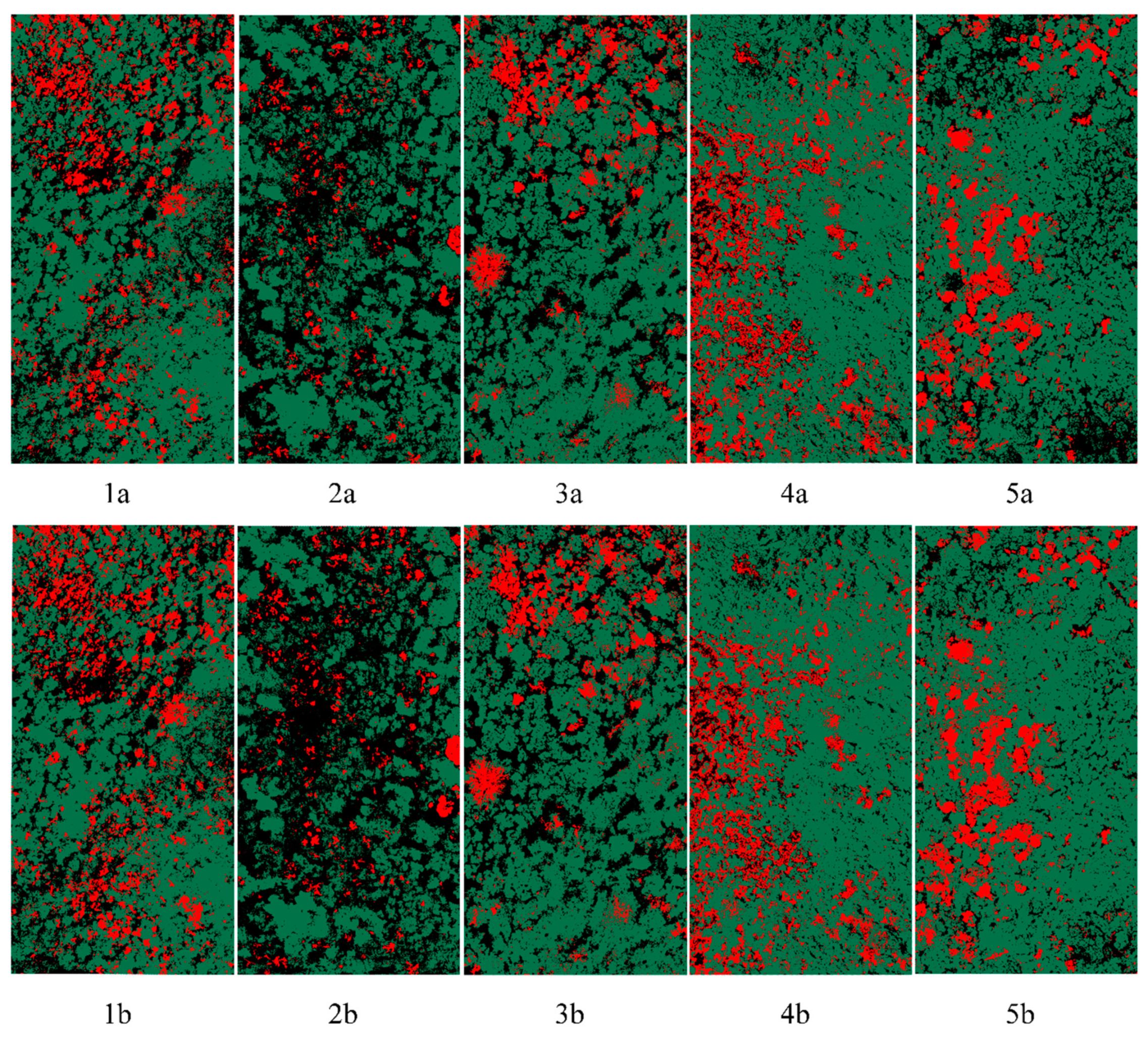
Classification results of the extent of the dead woody components in the five plots, marked in red and using the random forest algorithm results as an example. Plots: lot #1a-b, plot #2a-b, plot #3a-b, plot #4a-b, plot #5a-b. Top row: specific model. Bottom row: general model.
Figure 6.
Classification results of the extent of the dead woody components in the five plots, marked in red and using the random forest algorithm results as an example. Plots: lot #1a-b, plot #2a-b, plot #3a-b, plot #4a-b, plot #5a-b. Top row: specific model. Bottom row: general model.


Table 1.
Description of the five forest plots surveyed on the estimation of dead woody components at the Santa Rosa National Park Environmental Monitoring Super Site, Costa Rica.
Table 1.
Description of the five forest plots surveyed on the estimation of dead woody components at the Santa Rosa National Park Environmental Monitoring Super Site, Costa Rica.
| Plot | Secondary Succession | Description |
|---|---|---|
| 1 | Intermediate-intermediate | Forest patch contiguous to an old-grown forest patch and surrounded by early forests. The soils in this patch are shallow, with large exposures of volcanic rocks. |
| 2 | Early-intermediate | Forest composed of patches of grasses, shrubs, small deciduous trees and clusters of Quercus oleoides (white oak tree). |
| 3 | Intermediate-intermediate | Forest with two vegetation layers. The first layer encompasses deciduous tree species that reach a maximum height of 15 m. The second layer is below the canopy, composed of more shade-tolerant evergreen species and juveniles of many species. There is a high liana infestation. |
| 4 | Early-early | Forest patch with a low recovery located next to a firebreak. There is a high abundance of grasses, shrubs, small trees and large gaps. The maximum height of the trees is approximately 6–8 m. There is a high abundance of Madero negro (Gliricidia sepium), silk cotton tree (Cochlospermum vitifolium and), Yayo (Rehdera trinervis), as well as sun-loving heliophytes. |
| 5 | Intermediate-intermediate | Forest patch surrounded only by similar successional stages. This area was intensively used as cattle pasture during the Hacienda epochs from the 1600s to 1960. |
Table 2.
The implemented machine learning models and their parameters. Abbreviations: Acron: acronym, Avail: available; Gen: general model.
Table 2.
The implemented machine learning models and their parameters. Abbreviations: Acron: acronym, Avail: available; Gen: general model.
| Model | Acron. | Parameters | Avail. Values | Plot | Gen | ||||
|---|---|---|---|---|---|---|---|---|---|
| 1 | 2 | 3 | 4 | 5 | |||||
| Support Vector Machines with Linear Kernel | SVML | cost | c(1:100) | 55 | 56 | 19 | 1 | 3 | 62 |
| Support Vector Machines with Polynomial Kernel | SVMP | degree | c(1:10) | 3 | 4 | 1 | 6 | 5 | 5 |
| scale | seq(1,10,100) | 1 | 1 | 1 | 1 | 1 | 1 | ||
| C | c(1:100) | 2 | 10 | 14 | 6 | 1 | 24 | ||
| Support Vector Machines with Radial Kernel | SVMR | C | seq(1,10,100) | 1 | 6 | 1 | 8 | 3 | 2 |
| sigma | c(0.5:100) | 1 | 1 | 1 | 1 | 1 | 1 | ||
| Random Forest | RF | mty | c(1:100) | 1 | 1 | 60 | 2 | 4 | 2 |
| Conditional Inference Tree | CIT | maxdepth | c(1:100) | 3 | 9 | 4 | 16 | 2 | 13 |
| mincriterion | c(0.01:0.99) | 0.01 | 0.01 | 0.01 | 0.01 | 0.01 | 0.01 | ||
| C4.5-Like Trees | C45T | C | c(0.05:1) | 0.05 | 0.05 | 0.05 | 0.05 | 0.05 | 0.05 |
| M | c(1:100) | 1 | 1 | 3 | 1 | 1 | 1 | ||
| Gradient Boosting Machines | GMB | n.trees | c(1:100) | 56 | 97 | 31 | 97 | 97 | 96 |
| interaction.depth | c(1:10) | 10 | 10 | 6 | 10 | 1 | 10 | ||
| shrinkage | seq(0.1,0.5) | 0.1 | 0.1 | 0.1 | 0.1 | 0.1 | 0.1 | ||
| n.minobsinnode | c(5,7,10) | 10 | 10 | 5 | 5 | 5 | 10 | ||
| Neural Network | NNET | size | c(1:100) | 3 | 8 | 5 | 13 | 2 | 4 |
| decay | c(0.5:0.1) | 0.5 | 0.5 | 0.5 | 0.5 | 0.5 | 0.5 | ||
| Averaged Neural Network | ANNT | size | c(1:100) | 16 | 41 | 62 | 12 | 33 | 28 |
| decay | seq(0.01, 0.1, 0.5) | 0.01 | 0.01 | 0.01 | 0.01 | 0.01 | 0.01 | ||
| bag | seq(T, F) | T | T | T | T | T | T | ||
| Deep Neural Network | DNET | layer1 | c(1:10) | 3 | 10 | 7 | 4 | 2 | 10 |
| layer2 | c(1:10) | 1 | 8 | 9 | 5 | 10 | 6 | ||
| layer3 | c(0:10) | 8 | 2 | 0 | 1 | 0 | 6 | ||
| hidden_dropout | seq(0, 0.1) | 1 | 1 | 1 | 1 | 1 | 0 | ||
| visible_dropout | seq(0, 0.01) | 0 | 0 | 0 | 1 | 0 | 0 | ||
Table 3.
Average values of accuracy, kappa and processing times.
| Model | Accuracy | Kappa | Time (s) | |||
|---|---|---|---|---|---|---|
| Average | Stdev | Average | Stdev | Average | Stdev | |
| ANNT | 0.968 | 0.035 | 0.955 | 0.05 | 69,307.83 | 20,306.71 |
| CIT | 0.958 | 0.036 | 0.948 | 0.047 | 173.88 | 119.46 |
| C45T | 0.967 | 0.032 | 0.95 | 0.045 | 373.78 | 56.68 |
| DNET | 0.915 | 0.005 | 0.955 | 0.021 | 4970.45 | 3550.2 |
| GMB | 0.957 | 0.023 | 0.97 | 0.031 | 2839.38 | 2195.19 |
| NNET | 0.955 | 0.054 | 0.94 | 0.075 | 9271.34 | 5272.409 |
| RF | 0.98 | 0.02 | 0.958 | 0.034 | 1523.25 | 989 |
| SVML | 0.95 | 0.056 | 0.938 | 0.069 | 595.57 | 1066.37 |
| SVMP | 0.977 | 0.024 | 0.972 | 0.031 | 8188.28 | 11,149.98 |
| SVMR | 0.982 | 0.021 | 0.977 | 0.024 | 4689.92 | 8735.64 |
Abbreviations: Stdev = standard deviation.
Table 4.
Analysis of variance with repeated measures ANOVA of three performance variables (accuracy, kappa and processing time).
Table 4.
Analysis of variance with repeated measures ANOVA of three performance variables (accuracy, kappa and processing time).
| Degree Of Freedom (Df) | Sum Sq | Mean Sq | F Value | Pr (>F) | |
|---|---|---|---|---|---|
| ML Model | 9 | 1.370 | 4.667 | 150.000 | 0.000 |
| Residuals | 50 | ||||
| Accuracy Level | |||||
| ML Model | 9 | 0.009 | 0.001 | 0.886 | 0.004 |
| Residuals | 50 | 0.058 | 0.001 | ||
| Kappa Level | |||||
| ML Model | 9 | 0.009 | 0.001 | 0.484 | 0.879 |
| Residuals | 50 | 0.106 | 0.002 | ||
| Time Level | |||||
| ML Model | 9 | 23851 | 2650094356 | 40.132 | 0.000 |
| Residuals | 50 | 33017 | 66034978 | ||
Table 5.
Post hoc test p-values—Tukey multiple comparisons of means of the accuracy, kappa and time of ML models, with 95% confidence level.
Table 5.
Post hoc test p-values—Tukey multiple comparisons of means of the accuracy, kappa and time of ML models, with 95% confidence level.
| Accuracy | ||||||||||||
|---|---|---|---|---|---|---|---|---|---|---|---|---|
| ML Model | ANNT | CIT | C45T | DNET | GMB | NNET | RF | SVML | SVMP | SVMR | Means | Group |
| ANNT | 0 | 0.01 | 0.002 | 0.023 | 0.2 | 0.013 | 0.003 | 0.018 | 0.695 | 0.003 | 0.97 | 1 |
| CIT | 1 | 0 | 1 | 0.013 | 0.995 | 0.003 | 0.983 | 0.008 | 0.995 | 0.972 | 0.96 | 1 |
| C45T | 1 | 0.005 | 0 | 0.022 | 1 | 0.012 | 1 | 0.017 | 1 | 0.999 | 0.97 | 1 |
| GMB | 0.004 | 0.018 | 0.01 | 0.032 | 0 | 0.022 | 1 | 0.027 | 0 | 1 | 0.94 | 2 |
| DNET | 0.972 | 1 | 0.983 | 0 | 0.003 | 1 | 0.747 | 1 | 0.839 | 0.695 | 0.95 | 2 |
| NNET | 1 | 1 | 1 | 0.01 | 0.983 | 0 | 0.956 | 0.005 | 0.983 | 0.936 | 0.96 | 1 |
| RF | 0.012 | 0.022 | 0.013 | 0.035 | 0.003 | 0.025 | 0 | 0.03 | 0.003 | 1 | 0.98 | 1 |
| SVML | 0.995 | 1 | 0.004 | 0.005 | 0.936 | 1 | 0.002 | 0 | 0.003 | 0.003 | 0.95 | 2 |
| SVMP | 0.008 | 0.018 | 0.01 | 0.032 | 1 | 0.022 | 1 | 0.027 | 0 | 1 | 0.98 | 1 |
| SVMR | 0.013 | 0.023 | 0.015 | 0.037 | 0.005 | 0.027 | 0.002 | 0.032 | 0.005 | 0 | 0.98 | 1 |
| Time | ||||||||||||
| ML Model | ANNT | CIT | C45T | DNET | GMB | NNET | RF | SVML | SVMP | SVMR | Means | Group |
| ANNT | 0 | 69,133.95 | 68,934.05 | 64,337.38 | 66,468.45 | 60,036.5 | 67,784.59 | 68,712.26 | 61,119.55 | 64,617.92 | 69,307.83 | 3 |
| CIT | 0 | 0 | 1 | 0.989 | 1 | 0.643 | 1 | 1 | 0.786 | 0.993 | 173.88 | 1 |
| C45T | 0 | 199.898 | 0 | 0.992 | 1 | 0.671 | 1 | 1 | 0.809 | 0.995 | 373.78 | 1 |
| DNET | 0 | 4796.568 | 4596.67 | 0 | 2131.068 | 0.995 | 3447.202 | 4374.878 | 0.999 | 280.532 | 4970.45 | 2 |
| GMB | 0 | 2665.5 | 2465.602 | 1 | 0 | 0.93 | 1316.133 | 2243.81 | 0.978 | 1 | 2839.38 | 2 |
| NNET | 0 | 9097.455 | 8897.557 | 4300.887 | 6431.955 | 0 | 7748.088 | 8675.765 | 1083.05 | 4581.418 | 9271.33 | 2 |
| RF | 0 | 1349.367 | 1149.468 | 0.999 | 1 | 0.816 | 0 | 927.677 | 0.915 | 1 | 1523.24 | 1 |
| SVML | 0 | 421.69 | 221.792 | 0.995 | 1 | 0.701 | 1 | 0 | 0.833 | 0.997 | 595.57 | 1 |
| SVMP | 0 | 8014.405 | 7814.507 | 3217.837 | 5348.905 | 1 | 6665.038 | 7592.715 | 0 | 3498.368 | 8188.28 | 2 |
| SVMR | 0 | 4516.037 | 4316.138 | 1 | 1850.537 | 0.992 | 3166.67 | 4094.347 | 0.999 | 0 | 4689.91 | 2 |
Table 6.
Analysis of variance of the coverage of dead woody components of the five plots of the study area.
Table 6.
Analysis of variance of the coverage of dead woody components of the five plots of the study area.
| Df | Sum Sq | Mean Sq | F Value | Pr (>F) | |
|---|---|---|---|---|---|
| Plots | 4 | 1.29E-29 | 3.23E-30 | 3.296 | 0.046 |
| Residuals | 2 | 1.96E-30 | 9.81E-31 |
Table 7.
Tukey post hoc test—p-values results of the dead component coverage across the five plots of the study at SR-EMSS.
Table 7.
Tukey post hoc test—p-values results of the dead component coverage across the five plots of the study at SR-EMSS.
| Plot | 1 | 2 | 3 | 4 | 5 | Mean | Group |
|---|---|---|---|---|---|---|---|
| 1 | 0.000 | 9.100 | 3.450 | 0.089 | 0.050 | 13.45 | a |
| 2 | 0.000 | 0.000 | 0.004 | 0.000 | 0.000 | 4.35 | c |
| 3 | 0.034 | 5.650 | 0.000 | 0.003 | 0.036 | 10 | b |
| 4 | 2.650 | 11.750 | 6.100 | 0.000 | 2.700 | 16.1 | a |
| 5 | 1.000 | 9.050 | 3.400 | 0.083 | 0.000 | 13.4 | a |
© 2020 by the authors. Licensee MDPI, Basel, Switzerland. This article is an open access article distributed under the terms and conditions of the Creative Commons Attribution (CC BY) license (http://creativecommons.org/licenses/by/4.0/).
Share and Cite
MDPI and ACS Style
Campos-Vargas, C.; Sanchez-Azofeifa, A.; Laakso, K.; Marzahn, P. Unmanned Aerial System and Machine Learning Techniques Help to Detect Dead Woody Components in a Tropical Dry Forest. Forests 2020, 11, 827. https://doi.org/10.3390/f11080827
AMA Style
Campos-Vargas C, Sanchez-Azofeifa A, Laakso K, Marzahn P. Unmanned Aerial System and Machine Learning Techniques Help to Detect Dead Woody Components in a Tropical Dry Forest. Forests. 2020; 11(8):827. https://doi.org/10.3390/f11080827
Chicago/Turabian StyleCampos-Vargas, Carlos, Arturo Sanchez-Azofeifa, Kati Laakso, and Philip Marzahn. 2020. "Unmanned Aerial System and Machine Learning Techniques Help to Detect Dead Woody Components in a Tropical Dry Forest" Forests 11, no. 8: 827. https://doi.org/10.3390/f11080827
Note that from the first issue of 2016, this journal uses article numbers instead of page numbers. See further details here.