Spatial Estimation of the Latent Heat Flux in a Tropical Dry Forest by Using Unmanned Aerial Vehicles


1
Department of Geography, Ludwig-Maximilian University Munich, Luisenstrasse 37, 80333 Munich, Germany
2
Department of Geography, University of Lethbridge, Lethbridge, AB T1K3M4, Canada
3
Earth and Atmospheric Sciences Department, University of Alberta, Edmonton, AB T6G2E3, Canada
*
Author to whom correspondence should be addressed.
Forests 2020, 11(6), 604; https://doi.org/10.3390/f11060604
Submission received: 2 April 2020
/
Revised: 19 May 2020
/
Accepted: 20 May 2020
/
Published: 26 May 2020
(This article belongs to the Special Issue Forestry Applications of Unmanned Aerial Vehicles (UAVs) 2020)
Abstract
:In this paper, we address the retrieval of spatially distributed latent heat flux (E) over a tropical dry forest using multi-spectral and thermal unmanned aerial vehicle (UAV) imagery. The study was carried out in the Santa Rosa National Park Environmental Monitoring Super-Site, Costa Rica, in June 2016. The triangle method was used to derive E from the UAV imagery and the results were compared to E measurements of an eddy covariance system within the coincident eddy flux tower footprint. The tower footprint was derived using a two-dimensional parameterization model for flux footprint prediction. The comparisons with the flux tower measurements showed a mean relative difference of 10.98% with a slight overestimation of the UAV-based flux retrievals by nearly 7.7 Wm. The results are in good agreement with satellite-based retrievals, as provided by the literature, for which the triangle method was initially developed and mostly used so far. This study proved to be a promising approach for transferring the triangle method to UAV imagery in ecosystems such as tropical dry forests. With the presented approach, new details in spatially distributed latent heat flux estimates at ultra-high resolution are now possible, thereby potentially closing the gap in spatial resolution between satellites and flux towers. Even more, it allows tracing the latent heat flux from single trees at leaf level. Besides, this approach also opens new perspectives for the monitoring of latent heat fluxes in tropical dry forests.
1. Introduction
In recent years remote sensing has become an important element to the provisioning of spatially distributed input data for Earth system models. With various global initiatives, such as the Essential Climate Variables (ECV) defined by the World Meteorological Organization (WMO) and the European Space Agency’s Climate Change Initiative (ESA-CCI), global monitoring programs through satellite data are envisaged. Space-borne remote sensing (RS) platforms contribute to global environmental monitoring. However, limitations of satellite systems due to technical capabilities set the boundaries for the temporal and spatial resolution of many data sets [1]. This is a limitation for the validation of emerging remote sensing products with wide disparities among ground truth data [2], especially where there are significant inconsistencies between sensor and ground-based information. This is evident for ECVs such as evapotranspiration; i.e., the latent heat flux (E). E is a key element for improving our understanding of climate-mediated changes of energy and water cycling at global to local scales. Knowledge about the spatial distribution of E is essential for many applications, such as water resource management, agriculture, and forestry. Abnormal changes in E can be caused by plant water stress and reduced plant vitality. Therefore, spatially explicit estimates of E are of high interest for decision makers, especially in tropical dry forests, where climate change might have a negative impact on tree vitality [3].
Spatially distributed E estimates are usually derived from satellite-based (e.g., MODIS, MERIS, or Landsat) data products that have pixel resolutions ranging from 90 to 1000 m [2,4,5]. These data products are often validated with measurements of E from eddy covariance (EC) systems. However, measurements of E using the common EC approach might be derived for a much smaller eddy flux footprint than the sizes of one of these pixels. This difference in spatial resolution could possibly introduce large uncertainties due to spatial scaling effects [6,7]. In addition, measurements of EC-based E represent an average value for the total predicted flux footprint rather than plant-specific information, while the flux footprint prediction in turn is a function of wind speed, wind direction, and sensor height above a given surface [8]. Therefore, there is a lack of spatially explicit E information of high spatial resolution that would enable the monitoring of latent heat fluxes of forest canopies, plant individuals, or plant compartments over larger areas than those measured in-situ, which could also be used to validate satellite-based E estimates.
One emerging source of remote sensing information with significant potential for the calibration and validation of ECVs is near-surface observation from, e.g., multi-spectral sensors attached to autonomous unmanned aerial vehicles (UAVs). According to [9], UAVs can be used for closing the gap in scale between field and satellite-based observations by offering more flexible spatial, temporal, and spectral resolutions, potentially allowing the retrieval of information on single individual plants or land-surfaces at leaf scale. In addition, UAVs provide the unique opportunity to integrate thermal infrared (TIR) and visible and near-infrared (VIS-NIR) sensors into one single platform at low cost. This enables larger scale mapping (<0.1 km) of thermal properties of sites that are aimed to support calibration and validation efforts of emerging satellites. Recently, studies have addressed the derivation of latent heat flux estimates from UAVs by using different approaches. For example, reference [10] estimated E based on a two-source energy balance model by integrating a thermal infrared sensor with a fixed-wing UAV. The study shows the feasibility of using high-resolution UAV products instead of satellite-based products as model input. The study of [11] used UAV-based multi-spectral and thermal infrared data to develop a high resolution spatial evapotranspiration system. Within their study, they retrieved actual crop evapotranspiration from five different evapotranspiration models. The best results were achieved when applying input variables based on vegetation indices such as the normalized difference vegetation index (NDVI). In contrast, refs. [10,12] used only thermal UAV imagery to derive the latent heat flux.
Usually, the models applied to retrieve E from remote sensing data can be grouped into contextual/scene-based models or pixel based models [13]. While the models of the first group require the reflectance and/or land surface temperature (LST) information from the whole image scene to derive a so-called hot/dry edge and cold/wet edge to constrain the retrievals, models of the latter group do not consider such information and thus need more input parameters [13]. However, contextual models need a broad variety of different reflectance values to define those dry and wet edges, which is usually a result of surface heterogeneity [14]. The triangle method, first introduced by [15], is a well-established method representing the contextual models, while the “two source energy balance” (TSEB) [16,17] and the “surface energy balance algorithm for land” (SEBAL) [18] represent the pixel-based models. According to [19], contextual models have been extensively tested over large areas with sufficient surface heterogeneity, which restricted their applicability to coarser resolution satellite data. This in turn impedes the validation due to the mismatch of in-situ footprints and the sensor’s spatial resolution, as elaborated by [2]. Using high-resolution UAV data would allow for a better understanding of the spatial distribution of E.
Recently, ref. [13] tested three different E flux retrieval approaches from thermal and red-green-blue (RGB) UAV imagery. Although they did not include the near-infrared (NIR) domain, they concluded that simpler models such as the one-source or the triangle method can produce similar results compared to more complex inversion schemes such as a two-source energy balance model [13]. In addition, reference [20] used a UAV-based triangle method approach to retrieve root zone soil moisture information. In [21], the authors used the same UAV and triangle method approach to retrieve land surface energy, water, and CO fluxes at very high resolution. However, development and validation of such models applied to UAV imagery taken in different ecosystems such as tropical dry forests are still ongoing research and pending.
To better understand spatially explicit E values of tropical dry forests at ultra-high resolution, we modeled E using UAV-based visible and thermal reflectance information and the triangle method approach. Modeled E results were compared to EC measurements of the E flux. The objectives of the presented study are
- To derive spatially distributed estimates of E;
- To show the performance of a contextual method (triangle method [22]) in high-resolution imagery in tropical dry forests;
- To trace the different contributions of E at tree and branch level in a tropical dry forest environment.
2. Methods
2.1. Study Site
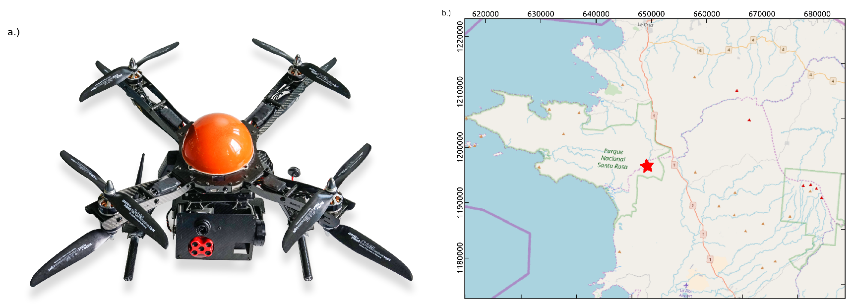
This study was carried out at the Santa Rosa National Park Environmental Monitoring Super-Site (SRNP-EMSS, Figure 1b). The SRNP-EMSS is located in the province of Guanacaste in the northwest of Costa Rica. The area has a mean annual temperature of 25 °C and receives a mean annual precipitation of 1750 mm. The dry season (December to May) remains rain free and marks the leaf-off period for about 90% of all trees. The tropical dry forest of Costa Rica, one of the most endangered ecosystems, consists of a mosaic of new-growth to old-growth forests depending on the year of agricultural abandonment, and as such has various forest structural properties and species [23]. The trees in the study area are on average about 18 m tall and have a relative age since abandonment of 30–35 years. The SRNP-EMSS hosts two EC systems plus four optical phenology stations, which have been in operation since 2013 [3]. The two EC systems have a distance of 1200 m. In addition, about 50 sensors are distributed within the footprints of both EC systems, measuring photosynthetic active radiation, temperature, relative humidity, and soil moisture. The UAV imagery that was acquired for this study is only coincident to one of these EC systems, due to difficulties of accessing the site and launching the UAV.
2.2. UAV and Camera Payload
2.2.1. UAV System
For this study, we used a Rotorkonzept-RKM 8X octocopter. The RKM 8X was designed by the German company Rotorkonzept and is a flexible lightweight UAV which can carry payloads up to 1100 g. The UAV is controlled by a Pixhawk flight controller which is an open hardware project, making it very flexible and extendable and allows to fly according to way-points. To fit the needs of simultaneously carrying two camera systems, a special two-axis stabilizing gimbal was built. The gimbal corrects for yaw and roll effects by using brush-less engines that allow an always nadir looking imaging geometry for both cameras. The mean flight duration of the RKM-8X is around 12 min with a payload of approximately 1000 g, depending on wind and humidity conditions. The nominal flight speed in standard flight mode is 5 m/s. The multi-spectral and thermal infrared cameras, described below, were mounted on the gimbal and complete the UAV system for the field experiments, as shown in Figure 1a.
UAV acquisitions were carried out at the 29th of June 2016 within four consecutive flights in order to cover a larger area of roughly 0.1 km. One of the four flights was directly coincident to the EC flux footprint and was carried out from 4:00 pm to 4:10 pm. The UAV images were acquired in autopilot mode in an altitude of 100 m above the canopy with a forward overlap of 80%, a sidelap of 70% between single images, and in nadir looking geometry. Image acquisition was carried out during constant overcast conditions.
2.2.2. Multi-Spectral Camera System
The Micasense RedEdge camera is a multi-rig camera allowing for the simultaneous acquisition of 5 channels. These 5 spectral bands are set up as an array of 2-1-2 containing the sensors from upper left to lower right: blue–near-infrared–rededge (middle)–green–red, covering the electromagnetic wavelength spectrum from visible to near-infrared. The band sensitivities differ from one to another, which needs to be addressed in the image pre-processing. Specifications of the Micasense RedEdge camera are shown in Table 1. Images are acquired with 12-bit depth and stored and saved as 16-bit tiff images for each channel separately in single files for further processing. To obtain calibrated images from the RedEdge, Micasense’s original calibration panel with highly Lambertian properties and known spectral albedo values was imaged before each flight and used for calibration inputs in the calibration procedure, as described in Section 2.4.1.
2.2.3. Thermal Camera System
The thermal infrared imagery was acquired using a FLIR TAU2 640. The TAU2 cores are manufactured to capture thermal video streams. In order to retrieve still imagery, the FLIR core was extended with a backend, designed by the German TEAX GmbH. The backend grabs the single frames from the video stream and converts it to a still image as a raw binary file of 14-bit.
2.3. Data
During the experiments, the following data Table 2 were acquired by the UAV, the EC system, and the wireless sensor network, as described in Section 2.1.
2.4. Camera Calibration
To convert the raw digital numbers (DNs) of the acquired imagery into real measurements, a calibration of both cameras was carried out. In the following, the approaches for the two camera systems are outlined in detail.
2.4.1. Multi-Spectral Camera System
The Micasense comes pre-calibrated and calibration values and constants were provided in the Exif-Header section of each raw tiff-file per band. In order to convert the raw 16-bit DNs into reflectance values, a calibration procedure was carried out according to Micasense recommendations. The calibration procedure included correcting for vignetting effects of the single camera lenses, black current compensation, and the conversion from radiance to reflectance by using a Lambertian calibration target with known spectral albedo values. For each flight, the calibration target was imaged with the Micasense camera assuming constant conditions of the atmosphere during the flight [24].
2.4.2. Thermal Camera System
The calibration of the FLIR TAU2 640 is relatively straightforward as it comes already calibrated off the shelf. A linear equation was used that allows the conversion of the DNs registered by the camera into degrees Celsius (°C) depending on the expected land surface temperature range. Equation (1) describes the conversion of DNs to °C for a so-called low gain case. This calibration was applied to all UAV digital terrain models (DTM) after orthomosaic generation. It is notable that the original FLIR camera stores the data in 14-bit DN, while the TEAX backend stores the imagery in 16-bit tiff format. Therefore, a conversion factor was implemented in Equation (1):
Under cloudy or overcast conditions the effect of emissivity on the thermal signal does not show any significant contribution and can be neglected according to [25]. Thus, no corrections for emissivity were carried out in this study. On average, the atmospheric column between the forest canopy and the UAV was 100 m in height above the canopy layer. The narrow atmospheric column minimizes the effects of scattering and absorption of radiation by atmospheric gases and aerosols on potential differences in the radiance that is reflected by the land surface and the radiance which is measured by the sensor [26,27]. Therefore, we decided to not atmospherically correct the thermal infrared data in this study. This decision was supported by the short flight time of less than 5 min, during which no changes in air temperature were observed, as indicated by simultaneous field measurements.
2.5. Orthomosaic Generation
The UAV orthomosaics were generated by using the individually calibrated images in the Agisoft Photoscan Professional software package (v1.3.2) (Agisoft LLC, St. Petersburg, Russia). Note that we used already radiometrically-calibrated images to have full control over the calibration procedure. Consequently, for the stitching of the single imagery, we used Agisoft without any further radiometric altering/filtering. To enhance the positional accuracy of the final orthomosaic, five full ground control points (GCPs) were measured in the field using a differential GPS (Trimble GeoXT6000, (Trimble Inc., Sunnyvale, CA, USA)) with an average horizontal error of 0.50 m and an average vertical accuracy of 0.54 m. These marked GCPs were included in the Agisoft workflow and enhanced the accuracy of the aligned image positioning significantly. To obtain a common resolution between the VIS-NIR and TIR orthomosaics, the derived TIR orthomosaic was oversampled by a factor of roughly two.
2.6. Derivation of Latent Heat Flux Using the Semi-Empirical Triangle Method
The triangle method introduced by [15] and further developed by [22,28] is a widely used approach [14,29,30,31,32] based on the Priestley–Taylor Equation (2) for the estimation of the E flux [Wm] with the energy balance equation of the following form:
where is a dynamical equivalent to the dimensionless Priestley–Taylor coefficient [-] [22,29], replacing the resistance terms of the Penman–Monteith Equation. is derived in the following by Equation (6). is the net radiation [Wm], G is the soil heat flux [Wm], is the slope of the saturated pressure curve derived after [33] [kPa K], and is the psychromatic constant derived after [34] in [kPa K]. The theory implies that a high E flux provides cooling of the surface area resulting in a cooler sunlit vegetation surface compared to a surface consisting of bare soil under similar conditions [14]. In comparison to the well-known SEBAL approach [16,18], fewer input variables are required and thus fewer sources of uncertainties are obtained. Although the triangle method approach was performed using predominantly satellite remote sensing products as model input variables [22,29,30,31,32], this study uses the approach with input variables derived from the aforementioned UAV-based VIS-NIR and TIR data sets. The VIS-NIR orthomosaic is hereby used to obtain the vegetation index, while the TIR orthomosaic provides the LST information. To derive E according to the approach proposed by [22], the NDVI is typically used. However, the near-infrared sensor of the Micasense camera showed high saturation effects across the acquired UAV imagery due to the vitality of a majority of the trees. For this study, the NDVI can not represent the fine spatial differences of vegetation greenness and results in a homogeneous land surface. A heterogeneous observation area is, however, one main requirement for the application of the triangle method [14,22,29]. Therefore, the NDVI was replaced by the rededge NDVI (RENDVI, [35,36]) which is defined as:
where the rededge band is used instead of the NIR band due to the sensitivity of the rededge band to small changes in canopy foliage content, gap fraction, and vegetation senescence. According to [36], the allowed ranges of wavelengths within the RENDVI are 670–740 nm for the rededge band and 663–673 nm for the red band, respectively. With 712–722 nm and 600–699 nm spectral bandwidth, the Micasense’s rededge and red band perfectly match the allowed ranges. With the spatially distributed RENDVI and LST maps, the Priestley–Taylor coefficient is derived. For the calibration of the semi-empirical model, this parameter can be scaled between and by linearly interpolating and (adjusted after [33]). The so obtained range of represents the maximum and minimum values for E such that the minimal value of E implies a minimum value of [29]. Potential evapotranspiration (ET) conditions occur when no plant-water stress is present, and therefore E can reach maximal values [22]. This is modeled by the wet-edge representing a maximum value of and thus of E. The true dry-edge is obtained when E is absent and thus zero, whereas an observed dry-edge represents limited E values with limited . In order to model increased E over higher vegetated areas in comparison to areas of sparse vegetation cover, a non-linear scaling of is performed with the following equation:
where represents for each pixel i and RENDVI value, and is according to [22] given by:
Based on this equation, the next step spreads the RENDVI-LST triangular space to the minimum and maximum extent of evaporative cooling, represented by , , and , for each RENDVI value i respectively [29,30]. The specific value is obtained by:
where represents the Priestley–Taylor coefficient for a specific RENDVI value i; LST and LST are the corresponding minimum and maximum LSTs; and is the observed surface temperature at pixel i.
The triangle method was conducted within R [37] using the R-package “Triangle Method”—which was freely provided by the author of the package [38] on demand. The additional inputs of air temperature, soil heat flux, and net radiation were provided by the EC system and the wireless-sensor network [3]. Although the EC system was covered by one flight line only, E was derived for the one full scene consisting of all four flight lines in order to capture a higher land-cover heterogeneity.
2.7. E-Flux Measurements and Footprint Estimation
Flux equipment was installed on a horizontal boom at a height of 35 m above the forest floor and in the footprint of the tower; e.g., soil heat flux. Different corrections for, e.g., time-lags, high frequency losses, and outlier detection were applied according to [3], and fluxes (CO, HO, momentum, and energy) were calculated as 30-min block averages of the 10 Hz single measurement intervals. According to [3] and after additional testing, a 30-min averaging of the 10 Hz intervals allowed an adequate capture of low-frequency fluxes. For this study, only the HO, momentum, and energy fluxes were used. E was calculated as the product of the latent heat of vaporization and the water vapor flux, expressed in energy units (Wm) [3].
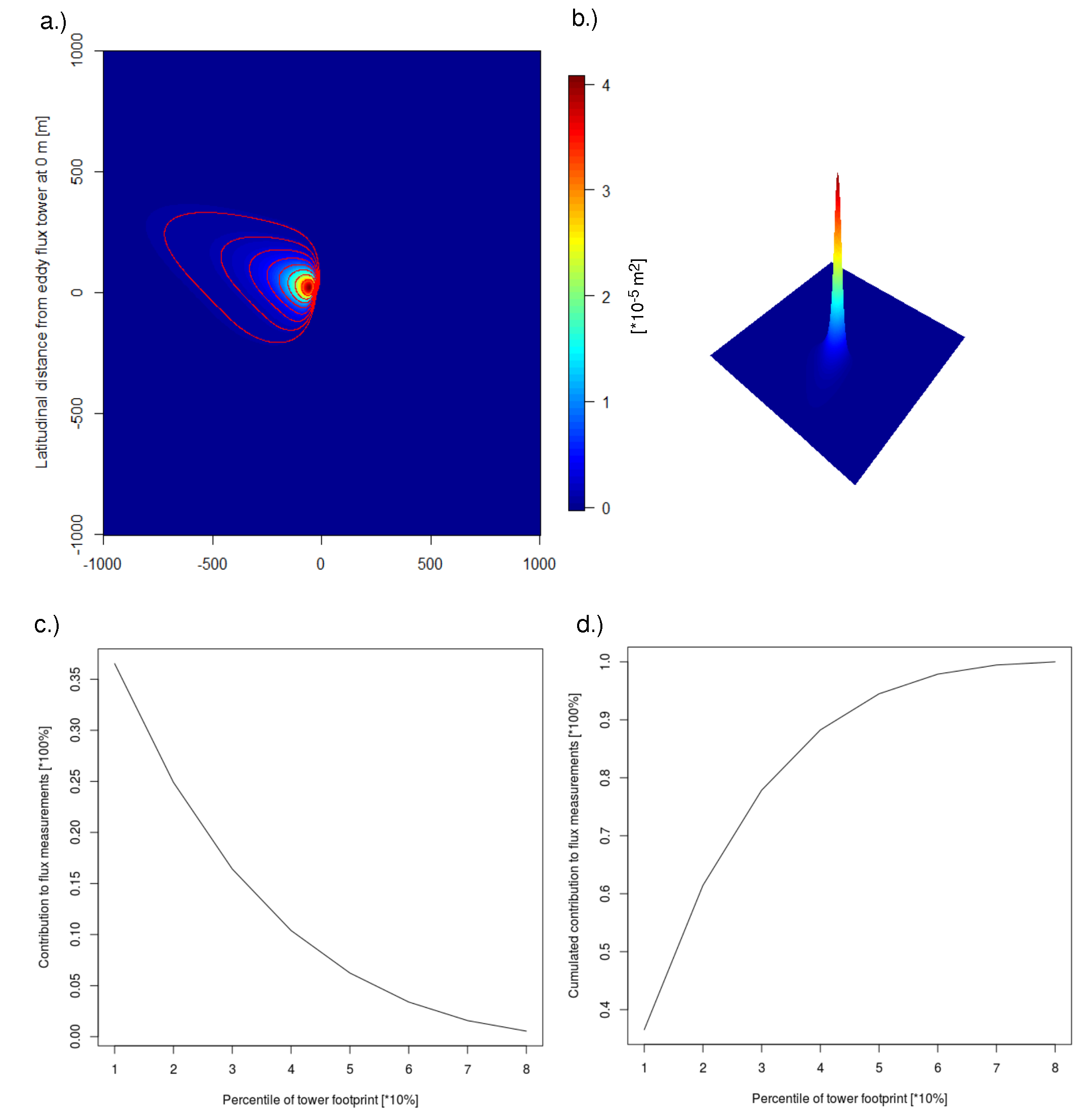
The EC footprint was derived using a two-dimensional parameterization of flux footprint prediction (FFP), developed by [39] as a one-dimensional approach and elaborated by [8] as a two-dimensional parameterization. The FFP models the spatial extents, widths, and shapes of weighted eddy fluxes per pixel in 1 m × 1 m increments using the measurements of the installed EC system within the test-site as inputs. Figure 2a,b) shows the output of the FFP. The FFP output is a grid of the spatio-temporal EC flux footprint, where each 1 m pixel is weighted based on its probability of contributing to the total flux measurement, the so-called probability density function (PDF). The extent and location of an area that contributes with a certain percentage to the total measured flux can be obtained [7,8]. The x and y coordinates in the model intern footprint coordinate system describe the distance to the source of measurement (EC system) in the specific direction. The value of the pixel in m describes the area cumulated under the integral in the specific class between 0 and 0.99 with 0.1 increments based on the PDF. The model was applied by using the open-source FFP algorithm in R, which is provided by [8].
Figure 2 illustrates the EC footprint area divided into its PDF contributions, derived with a 30 min average sampling rate temporally coincident to the UAV flight overpass. The upper two images of Figure 2 visualize the distribution in a two-dimensional and three-dimensional directions. The color scheme and the extent in z direction respectively, indicate the contribution to the total measured flux within the specific weighted class of probability, precisely a part of the area [m] below the integral of the PDF. Due to the limited battery capacity of the UAV, the observation area covers the EC footprint only for a footprint area where 63% of the total measured flux originates (red and yellow ellipses in Figure 2a). Thus, it represents more than half of the complete measured flux (Figure 2c,d). As the rest of the flux contributing footprint area lies outside the UAV coverage, only this area is used for validation purposes. Therefore, the modeled E raster file was cropped to the size of the specific footprint of the time and day.
2.8. Validation of E Retrievals
For the validation of the UAV based E retrievals, the measurements of the EC systems were used. In particular, as mentioned in Section 2.7, the mean over all the pixels within the considered footprint was benchmarked against the measurements of the EC system. For the accuracy assessment, the mean absolute difference and the mean relative difference were calculated.
3. Results
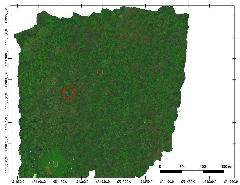
Figure 3 shows the VIS-NIR orthomosaic in true-color representation for the complete study area and for the region of interest (Figure 4).
The spatial resolution of the VIS-NIR orthomosaic is 0.08 m and consists in total of 437 single images that were aligned successfully. While 10% of the total 437 TIR images could not be aligned due to insufficient contrast in the images, we were able to close specific alignment gaps due to the applied forward overlap of 80% during the UAV image acquisition. Consequently, VIS-NIR and thermal orthomosaics have been produced without any spatial gaps. With a positional accuracy of below one pixel (less than two times the spatial resolution), the VIS-NIR orthomosaic is of high qualtiy [40,41]. The co-registration of the VIS-NIR and TIR orthomosaics through cross-correlation resulted in 93 tie-points and after applying a polynomial shift in a RMSE of 0.0014 m.
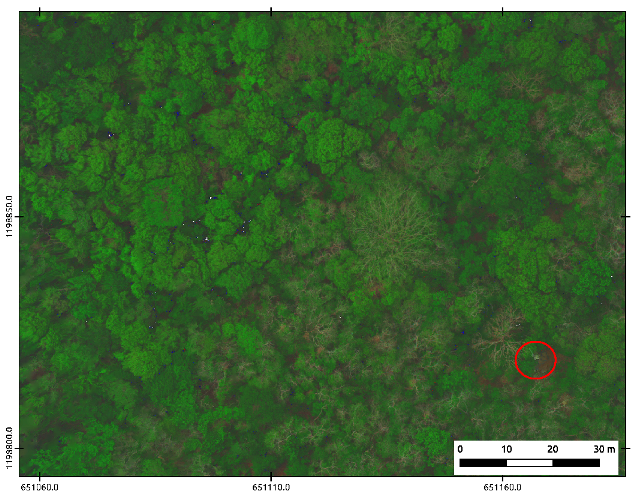
In general, different landscape features, such as roads, clearings, single trees, and even single branches, are visible. For further analysis, the generated orthomosaics have been cropped to the estimated footprint of the EC system, as shown in Figure 5 and Figure 6.
The simultaneously measured E flux of the EC-station is 70.2 Wm. With a mean absolute difference of 7.7 Wm of the modeled UAV-based E, the triangle method approach slightly overestimates the measured flux with a mean relative difference of 10.98%.
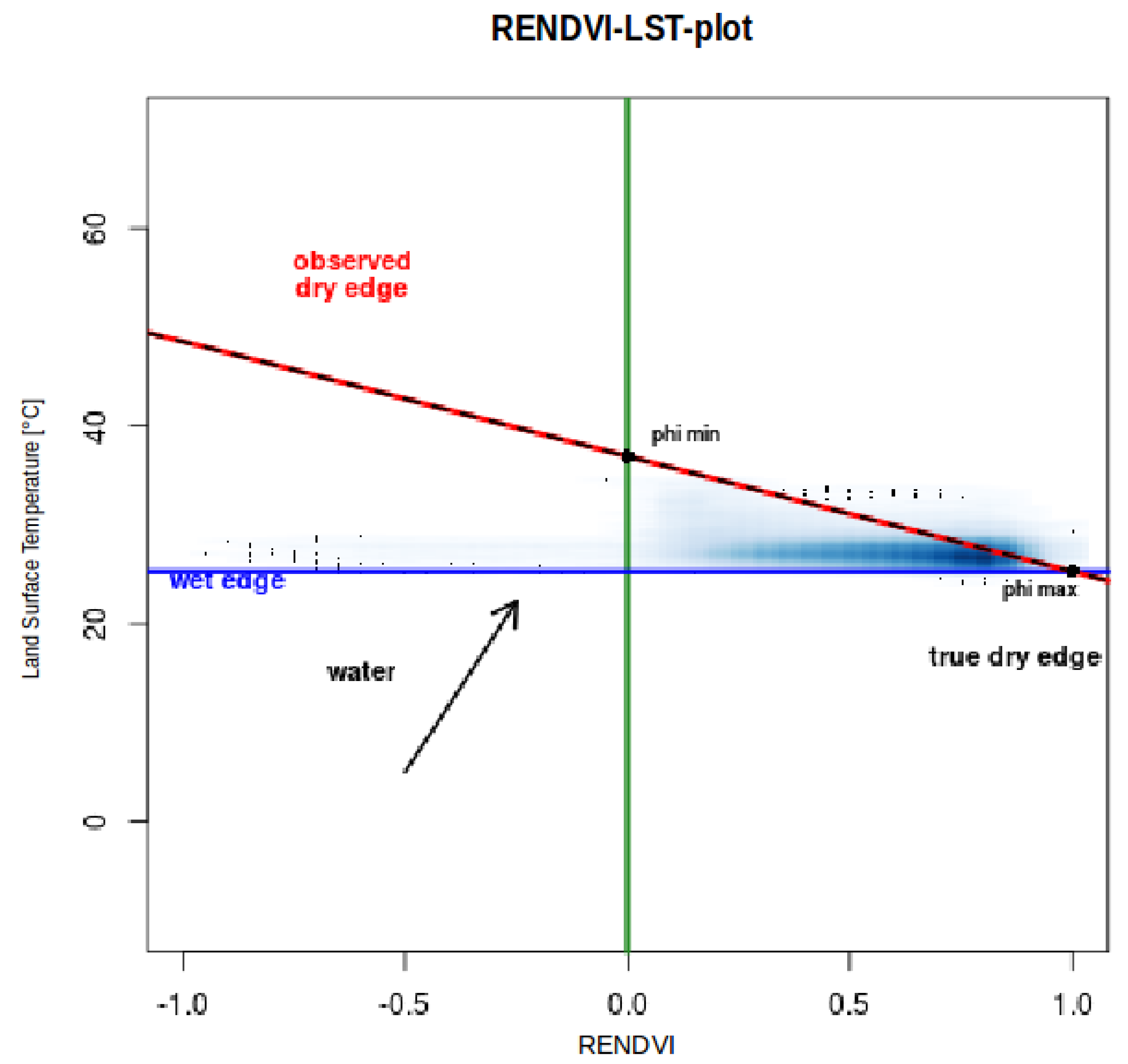
Figure 7 shows the corresponding RENDVI-LST triangle plot for the retrieved E estimates. Note that the plot was calculated from the total covered flight area to ensure a maximum heterogeneity of the LST and RENDVI pixel values [22,29]. In this plot, the clustering of the pixel values for RENDVI and LST around the right corner of the not ideally developed triangle is clearly visible. This indicates near-potential evapotranspiration conditions along the wet-edge with low LST and high RENDVI values and leads to a saturation of the spatially distributed E estimates.
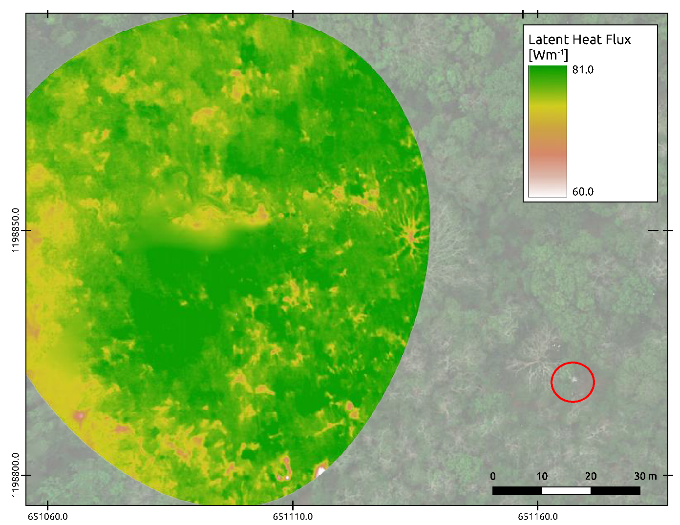
The modeled spatially explicit E estimates are illustrated in Figure 8 and are cropped to the coincident EC footprint area (Figure 8). Due to the high spatial resolution of the UAV data sets, even single trees and individual branches can be detected. In general, lower values of E correspond to the open patches of soil and leafless tree branches while higher values correspond to fully developed and vital vegetation that show nearly potential evapotranspiration. This is indicated by the RENDVI-LST-plot from Figure 7, and in particular, by the clustering at low LST and high RENDVI values. However, shadowed forest areas, forest occlusion, and understory vegetation also indicate high values in E close to potential evaporation. This can be observed especially in the center of the E footprint. A zoomed-in analysis reveals the spatial differences due to the different trees and leaf conditions. Even the more productive parts of single trees can be distinguished from dry or dead branches, which reduce the latent heat flux significantly. In addition, branches of liana infested trees, which are very common in that area [42], can be detected by reduced values of E. As lianas develop more woody biomass [27] and thus consequently reduce the fraction of E of a canopy surface. This is especially visible in the eastern part of the footprint, where a larger liana infested tree shows reduced E values.
4. Discussion
Within this paper, UAV-based estimates of the latent heat flux (E) have been carried out using a VIS-NIR and a TIR orthomosaic in combination with a conceptual model—the triangle method-over a tropical dry forest in Costa Rica. Comparisons to actual in-situ measurements using an EC system showed a good accuracy of the approach with an absolute error of 7.7 Wm and a relative error of 10.98%. With this approach, E estimates are traceable to individual tree, allowing one to distinguish between leafless branches of trees, dead trees, and lianas. Although further ground-truthing needs to be conducted, the proposed approach seems to be promising for advancing the analysis of liana distribution and development, a topic that is highly relevant with expected climate-mediated increases in liana abundance in tropical dry forests [23,42].
However, the retrieval of E by using the triangle method was challenging due to the relatively homogeneous surface area. As described in [22,29], the triangle method provides the best results when the imaged surface is heterogeneous. Consequently, the LST-RENDVI triangle did not develop properly in comparison to other studies that surveyed a more heterogeneous surface area. In addition, our results show that the forest mostly shaded the soil surface due to its dense canopy layer. Therefore, near-potential evaporation was derived for most of the area besides some gravel roads, trails, and dead trees or woody biomass. However, this might be an overestimation because inherently shaded areas are cooler, which potentially could result in the false indication of higher E values that lead to potential evapotranspiration. Nevertheless, the retrieved results of this study are in good accordance with other studies that use UAV or satellite-based estimates of E [4,13,22,29,32,33,43]. The proposed approach provides, therefore, a very flexible method for the monitoring of spatially-distributed E fluxes complementary to EC measurements with a clear focus on the characterization of spatially explicit sub-footprint fluxes.
A further critical step of the proposed study was the co-registration of the VIS-NIR and TIR imagery. For the alignment, a large number of GCPs were drived in order to provide exact matching of the two orthomosaics. GCPs thereby consisted predominantly of intersecting branches that showed different thermal signals compared to the background information. Since placing the GCPs in the orthomosaics is time-consuming, cost-intensive, and in the case of this study challenging in a forest canopy dominated area, reference [41] developed an automatic co-registration procedure for multi-temporal and high-resolution UAV image data sets, without the use of GCPs. By doing so, the results are comparable to those using the manual strategy, resulting in reliable results [41]. The development of such a fully automatic processing chain would have been an advantage. However, such an implementation for the integration of a VIS-NIR with a TIR camera is not yet available. Besides, future implementations of such an algorithm should also consider the x, y and z-shifts of the two camera systems in order to overcome the co-registration problem.
Other sources of uncertainty are the flight duration and therewith the changing environmental conditions and the saturation of the NDVI. To address the changing environmental conditions, a reflectance calibration of the VIS-NIR data is crucial. Reference [44] outline that a change in illumination can be neglected for flights less than 15 min. However, continuous reflectance measurements in a one-minute interval revealed changing conditions even within such a short flight period for our study. Therefore, refs. [24,44] concluded that best reflectance calibration results are achieved using the continuous panel method by either recording spectral responses of a Lambertian surface with a spectrometer throughout the flight time and across the area of interest, or by mounting an incoming irradiance measurement device, e.g., Micasense’s day-light-sensor (DLS), on top of the UAV. Reference [9] also emphasizes the importance of a continuous reflectance calibration method. So far, first attempts of integrating the DLS with our UAV system only showed small changes in reflectance responses. However, further field experiments need to be conducted to explore the possibilities of the DLS sensor. In order to address the saturation effects of the NDVI above fully developed forest canopies [43], which predominantly originate from the saturation of the NIR band of the Micasense camera, modifications of the triangle method were conducted by exchanging the NDVI with the RENDVI. This modification was successful for the described UAV system setup and is recommended for similar studies. Furthermore, the triangle method approach requires only a small amount of measured input parameters in addition to the UAV input data sets, which makes this approach very suitable for E retrievals and facilitates applications also in data scarce areas [31,32].
Looking forward, the applied and tested method can pave the way for the integration of UAV systems in a multi-data analysis approach. Hereby, the proposed approach could function as a gap closure between different spatial and temporal scales which could also be used for the validation of remote sensing based E products across different scales [9]. As shown in Figure 2, the estimated E flux of a coarse resolution remote sensing product (e.g., MODIS 500 m × 500 m resolution) can be highly biased if compared to a time series of flux footprint measurements. Assuming that such a MODIS pixel would integrate all pixels of one scene to a single value, the UAV-based approach reveals much more detail, exceeding spectral mixing analysis as well, which can be seen in Figure 8.
Furthermore, thanks to the high spatial resolution of the UAV imagery, the proposed approach can be regarded as a complementary source of information compared to traditional EC measurements. Because EC measurements perfectly match the field scale but only provide rough estimates of the flux contributing areas, new insights are provided in our study. Here we were able to trace the single individual flux contributions (e.g., trees, branches, leaves, gaps) to the total flux as measured by the EC system. Our study is therefore of great value for understanding spatially explicit flux contributions in ultra-high spatial resolution as shown in Figure 2 and Figure 8. The added value lies in particular in the characterization of the different forest constitutions, such as tree species or fraction of liana infested or dead trees.
5. Conclusions
In this paper, a study is introduced which used UAV-based VIS-NIR and TIR data in combination with a contextual semi-empirical model for the retrieval of spatially explicit latent heat flux information. It was demonstrated that E retrievals with a mean relative difference of 10.98% can be achieved using such a setup over a tropical dry forest. This is of great value, especially as the tropics are often prone to cloud coverage, and thus satellite-based retrievals of E are limited. Furthermore, UAV-based, spatially-distributed latent heat estimates derived with the semi-empirical triangle method over a tropical dry forest are so far unique and allow the provision of new insights into spatially-distributed fluxes and their corresponding footprints, especially when using advanced camera systems such as a multi-spectral and a thermal camera system flown simultaneously on a UAV. By doing so, this paper demonstrates the derivation of reliable E estimates in an ultra-high spatial resolution. The applied method closes the gap in scale between space-borne remote sensing products and ground-based flux measurements. Consequently, it allows tracing the spatially-distributed, individual flux contributions from individual trees, branches, and leaves to the total flux in much greater detail. This is evident, especially when compared to the currently available flux footprint estimation tools or satellite remote sensing products, and thus adds complementary details of great value to current flux studies. Finally, the proposed approach provides a future method for monitoring the changing tropical dry forests of the SRNP-EMSS in Costa Rica in terms of tracking changes in evapotranspiration due to an increase in the fraction of liana infested trees.
Author Contributions
P.M. and L.F. both contributed to the writing of the paper and processed the data. P.M. acquired the UAV data. A.S.-A. is the PI of the SRNP Flux site and contributed to the writing of the paper. All authors have read and agreed to the published version of the manuscript.
Funding
This research was supported by the Inter-American Institute for Global Change Research, Collaborative Research Network Program (CRN3-025 Tropi-Dry) and the National Science and Engineering Research Council of Canada (NSERC) - Discovery Grant Program.
Acknowledgments
The authors would like to thank Brad Daniels for providing dGPS measurements of the GCP data and Saulo Castro for processing the flux tower data.
Conflicts of Interest
The authors declare no conflict of interest.
References
- Fischer, J.; Melton, F.; Middleton, E.; Hain, C.; Anderson, M.; Allen, R.; McCabe, M. The Future of Evapotranspiration. Global requirements for ecosystem functioning, carbon and climate feedbacks, agricultural management, and water resources. Water Resour. Res. 2017, 53, 2618–2626. [Google Scholar] [CrossRef]
- Loew, A.; Bell, W.; Brocca, L.; Bulgin, C.E.; Burdanowitz, J.; Calbet, X.; Donner, R.V.; Ghent, D.; Gruber, A.; Kaminski, T.; et al. Validation practices for satellite-based Earth observation data across communities. Rev. Geophys. 2017, 55, 779–817. [Google Scholar] [CrossRef] [Green Version]
- Castro, S.M.; Sanchez-Azofeifa, G.A.; Sato, H. Effect of drought on productivity in a Costa Rican tropical dry forest. Environ. Res. Lett. 2018, 13, 045001. [Google Scholar]
- Venturini, V.; Bisht, G.; Islam, S.; Jiang, L. Comparison of evaporative fractions estimated from AVHRR and MODIS sensors over South Florida. Remote Sens. Environ. 2004, 93, 77–86. [Google Scholar] [CrossRef]
- de Tomás, A.; Nieto, H.; Guzinski, R.; Salas, J.; Sandholt, I.; Berliner, P. Validation and scale dependencies of the triangle method for the evaporative fraction estimation over heterogeneous areas. Remote Sens. Environ. 2014, 152, 493–511. [Google Scholar] [CrossRef]
- Jakob, S.; Zimmermann, R.; Gloaguen, R. The need for accurate geometric and radiometric corrections of drone-borne hyperspectral data for mineral exploration: MEPHySTo—A toolbox for pre-processing drone-borne hyperspectral data. Remote Sens. 2017, 9, 88. [Google Scholar]
- Sutherland, G.; Chasmer, L.; Kljun, N.; Devito, K.; Petrone, M. Using High Resolution LiDAR Data and a Flux Footprint Parametrization to Scale Evapotranspiration Estimates to Lower Pixel Resolution. Can. J. Remote Sens. 2017, 43, 215–229. [Google Scholar] [CrossRef] [Green Version]
- Kljun, N.; Calanca, P.; Rotach, M.W.; Schmid, H.P. A simple two-dimensional parameterisation for Flux Footprint Prediction (FFP). Geosci. Model. Dev. 2015, 8, 3695–3713. [Google Scholar] [CrossRef] [Green Version]
- Gamon, J. Reviews and Syntheses: Optical sampling of the flux tower footprint. Biogeoscience 2015, 12, 4509–4523. [Google Scholar]
- Hoffmann, H.; Nieto, H.; Jensen, R.; Guzinski, R.; Zarco-Tejada, P.; Friborg, T. Estimating evaporation with thermal UAV data and two-source energy balance models. Hydrol. Earth Syst. Sci. 2016, 20, 697–713. [Google Scholar]
- Chávez, J.; Hathaway, J. Developing an Unmanned Aerial Remote Sensing of ET System. In Proceedings of the ASABE Annual International Meeting, Orlando, FL, USA, 17–20 July 2016. [Google Scholar]
- Ortega-Farías, S.; Ortega-Salazar, S.; Poblete, T.; Kilic, A.; Allen, R.; Poblete-Echeverría, C.; Ahumada-Orellana, L.; Zuñiga, M.; Daniel, S. Estimation of Energy Balance Components over a Drip-Irrigated Olive Orchard Using Thermal and Multispectral Cameras Placed on a Helicopter-Based Unmanned Aerial Vehicle (UAV). Remote Sens. 2016, 8, 638. [Google Scholar] [CrossRef] [Green Version]
- Brenner, C.; Zeeman, M.; Bernhardt, M.; Schulz, K. Estimation of evapotranspiration of temperate grassland based on high-resolution thermal and visible range imagery from unmanned aerial systems. Int. J. Remote Sens. 2018, 39, 5141–5174. [Google Scholar] [CrossRef] [PubMed] [Green Version]
- Carlson, T. An Overview of the Triangle Method for Estimating Surface Evapotranspiration and Soil Moisture from Satellite Imagery. Sensors 2007, 7, 1612–1629. [Google Scholar] [CrossRef] [Green Version]
- Price, J. Using spatial context in satellite data to infer regional scale evapotranspiration. IEEE Trans. Geosci. Remote Sens. 1990, 28, 940–948. [Google Scholar] [CrossRef] [Green Version]
- Norman, J.M.; Kustas, W.P.; Humes, K.S. Source approach for estimating soil and vegetation energy fluxes in observations of directional radiometric surface temperature. Agric. For. Meteorol. 1995, 77, 263–293. [Google Scholar] [CrossRef]
- Kustas, W.P.; Anderson, M.C.; Alfieri, J.G.; Knipper, K.; Torres-Rua, A.; Parry, C.K.; Nieto, H.; Agam, N.; White, W.A.; Gao, F.; et al. The Grape Remote Sensing Atmospheric Profile and Evapotranspiration Experiment. Bull. Am. Meteorol. Soc. 2018, 99, 1791–1812. [Google Scholar] [CrossRef] [Green Version]
- Kustas, W.P.; Alfieri, J.G.; Anderson, M.C.; Colaizzi, P.D.; Prueger, J.H.; Evett, S.R.; Neale, C.M.U.; French, A.N.; Hipps, L.E.; Chávez, J.L.; et al. Evaluating the two-source energy balance model using local thermal and surface flux observations in a strongly advective irrigated agricultural area. Adv. Water Resour. 2012, 50, 120–133. [Google Scholar] [CrossRef] [Green Version]
- Xia, T.; Kustas, W.P.; Anderson, M.C.; Alfieri, J.G.; Gao, F.; McKee, L.; Prueger, J.H. Mapping Evapotranspiration with High-Resolution Aircraft Imagery over Vineyards Using One-And Two-Source Modeling Schemes. Hydrol. Earth Syst. Sci. 2016, 20, 1523–1545. [Google Scholar] [CrossRef] [Green Version]
- Wang, S.; Garcia, M.; Ibrom, A.; Jakobsen, J.; Josef Köppl, C.; Mallick, K.; Looms, M.; Bauer-Gottwein, P. Mapping Root-Zone Soil Moisture Using a Temperature–Vegetation Triangle Approach with an Unmanned Aerial System: Incorporating Surface Roughness from Structure from Motion. Remote Sens. 2018, 10, 1978. [Google Scholar] [CrossRef] [Green Version]
- Wang, S.; Garcia, M.; Bauer-Gottwein, P.; Jakobsen, J.; Zarco-Tejada, P.J.; Bandini, F.; Paz, V.S.; Ibrom, A. High spatial resolution monitoring land surface energy, water and CO2 fluxes from an Unmanned Aerial System. Remote Sens. Environ. 2019, 229, 14–31. [Google Scholar] [CrossRef]
- Jiang, L.; Islam, S. A methodology for estimation of surface evapotranspiration over large areas using remote sensing observations. Geophys. Res. Lett. 1999, 26, 2773–2776. [Google Scholar] [CrossRef] [Green Version]
- Sánchez-Azofeifa, G.; Guzmán-Quesada, J.; Vega-Araya, M.; Campos-Vargas, C.; Durán, S.; D’Souza, N.; Gianoli, T.; Portillo-Quintero, C.; Sharp, I. Can terrestrial laser scanners (TLSs) and hemispherical photographs predict tropical dry forest succesion with liana abundance. Biogeosciences 2017, 14, 977–988. [Google Scholar] [CrossRef] [Green Version]
- Miura, T.; Huete, A.R. Performance of three reflectance calibration methods for airborne hyperspectral spectrometer data. Sensors 2009, 9, 794–813. [Google Scholar] [CrossRef] [Green Version]
- Maes, W.; Steppe, K. Estimating evapotranspiration and drought stress with ground-based thermal remote sensing in agriculture: A review. J. Exp. Bot. 2012, 63, 4671–4712. [Google Scholar] [CrossRef] [PubMed] [Green Version]
- Iqbal, F.; Lucieer, A.; Barry, K. Simplified radiometric calibration for UAS-mounted multispectral sensor. Eur. J. Remote Sens. 2018, 51, 301–313. [Google Scholar] [CrossRef]
- Yuan, X.; Laakso, K.; Marzahn, P.; Sanchez-Azofeifa, G.A. Canopy Temperature Differences between Liana-Infested and Non-Liana Infested Areas in a Neotropical Dry Forest. Forests 2019, 10, 890. [Google Scholar] [CrossRef] [Green Version]
- Carlson, T.; Capehart, W.; Gillies, R. A new look at the simplified method for remote-sensing of daily evapotranspiration. Remote Sens. Environ. 1995, 54, 161–167. [Google Scholar] [CrossRef]
- Stisen, S.; Sandholt, I.; Nørgaard, A.; Fensholt, R.; Høgh Jensen, K. Combining the Triangle Method with thermal inertia to estimate regional evapotranspiration: Applied to MSG-SEVIRI data in the Senegal River basin. Remote Sens. Environ. 2008, 112, 1242–1255. [Google Scholar] [CrossRef]
- Tang, R.; Li, Z.; Tang, B. An application of the Ts-VI Triangle Method with enhanced edges determination for evapotranspiration estimation from MODIS data in arid and semi-arid regions—Implementation and validation. Remote Sens. Environ. 2010, 114, 540–551. [Google Scholar] [CrossRef]
- Meyer, S.; Blaschek, M.; Duttmann, R.; Ludwig, R. Improved hydrological model parametrization for climate change impact assessment under data scarcity: The potential of field monitoring teqhniques and geostatistics. Sci. Total Environ. 2016, 543, 906–923. [Google Scholar] [CrossRef]
- Gampe, D.; Ludwig, R.; Qahman, K.; Afifi, S. Applying the Triangle Method for the parametrization of irrigated areas as input for spatially distributed hydrological modeling: Assessing future drought risk in the Gaza Strip (Palestine). Sci. Total Environ. 2016, 543, 877–888. [Google Scholar] [CrossRef]
- Batra, N.; Islam, S.; Venturini, V.; Bisht, G.; Liang, L. Estimation and comparison of evapotranspiration from MODIS and AVHRR sensors for clear sky days over the southern Great Plains. Remote Sens. Environ. 2006, 103, 1–15. [Google Scholar]
- Wang, K.; Cribb, M. Estimation of evaporative fraction from a combination of day and night land surface temperatures and NDVI—A new method to determine the Priestley-Taylor parameter. Remote Sens. Environ. 2006, 102, 293–305. [Google Scholar] [CrossRef]
- Gitelson, A.; Merzlyak, M. Spectral Reflectance Changes Associated with Autumn Senescence of Aesculus Hippocastanum L. and Acer Platanoides L. Leaves. J. Plant Physiol. 1994, 143, 286–292. [Google Scholar] [CrossRef]
- Sims, D.; Gamon, J. Relationships Between Leaf Pigment Content and Spectral Reflectance Across a Wide Range of Species. Leaf Structures and Developmental Stages. Remote Sens. Environ. 2002, 81, 337–354. [Google Scholar] [CrossRef]
- R Core Team. R: A Language and Environment for Statistical Computing; R Foundation for Statistical Computing: Vienna, Austria, 2020. [Google Scholar]
- Gampe, D.; Huber-García, V.; Marzahn, P.; Ludwig, R. Estimating actual evapotranspiration from remote sensing imagery using R: The package’ TriangleMethod. In Proceedings of the EGU General Assembly Conference Abstracts, Vienna, Austria, 23–28 April 2017. Number 18636. [Google Scholar]
- Kljun, N.; Calanca, P.; Rotach, M.; Schmid, H. A simple parameterisation for flux footprint predictions. Bound. Layer Meteorol. 2004, 112, 503–523. [Google Scholar] [CrossRef]
- Mesas-Carrascosa, F.J.; Torres-Sánchez, J.; Peña, J.M.; García-Ferrer, A.; Castillejo-González, I.L.; López Granados, F. Generating UAV accurate ortho-mosaicked images using a six-band multispectral camera arrangement. In Proceedings of the 2014 RHEA Conference, Madrid, Spain, 20–22 May 2014. [Google Scholar]
- Aicardi, I.; Nex, F.; Gerke, M.; Lingua, A.M. An image-based approach for the co-registration of multi-temporal UAV image datasets. Remote Sens. 2017, 8, 779. [Google Scholar]
- Li, W.; Campos-Vargas, C.; Marzahn, P.; Sanchez-Azofeifa, A. On the estimation of tree mortality and liana infestation using a deep self-encoding network. Int. J. Appl. Earth Obs. Geoinf. 2018, 73, 1–13. [Google Scholar] [CrossRef]
- Vescovo, L.; Wohlfahrt, G.; Balzarolo, M.; Pilloni, S.; Sottocornola, M.; Rodeghiero, M.; Gianelle, D. New spectral vegetation indices based on the near-infrared shoulder wavelengths for remote detection of grassland phytomass. Int. J. Remote Sens. 2012, 33, 2178–2195. [Google Scholar] [CrossRef] [Green Version]
- Miura, T.; Huete, A.; Ferreira, L.; Sano, E.; Yoshioka, H. Hyperspectral Remote Sensing of Tropical and Sub-tropical Forests; Chapter A Technique for Reflectance Calibration of Airborne Hyperspectral Spectrometer Data Using a Broad, Multiband Radiometer; CRC Press: Boca Raton, FL, USA, 2008; pp. 213–232. [Google Scholar]
Figure 1.
(a) Rotorkonzept RKM-8X octocopter with Micasense RedEdge (red camera) and FLIR TAU2 640 (lens over the Micasense) placed in a two-axis stabilizing gimbal. (b) Location of the flux site within the Santa Rosa National Park Environmental Monitoring Super-Site (SRNP-EMSS), Costa Rica (map: Open Street Map).

Figure 2.
Derivation of a two-dimensional eddy covariance (EC) footprint with a sampling rate of 30 min average of the 29th of June 2016. (a) Extent of footprint from the EC system (at 0;0 m) in x and y directions, representing longitudinal and latitudinal distance [m] respectively; colors indicate the weighted PDF function [*10 m]. (b) Three-dimensional distribution with weighted PDF function in z direction [*10 m] of the same tower, (c) contributing flux [%] for percentiles of tower area, and (d) cumulated flux [%].

Figure 3.
True-color (RGB) VIS-NIR orthomosaic of the Micasense RedEdge camera providing an overview of the whole flight area. The red circle indicates the position of the EC system.
Figure 3.
True-color (RGB) VIS-NIR orthomosaic of the Micasense RedEdge camera providing an overview of the whole flight area. The red circle indicates the position of the EC system.

Figure 4.
Generated VIS-NIR orthomosaic as an overview of the tower area including the footprint of the EC system in RGB representation. Red circle indicates the position of the EC system.
Figure 4.
Generated VIS-NIR orthomosaic as an overview of the tower area including the footprint of the EC system in RGB representation. Red circle indicates the position of the EC system.

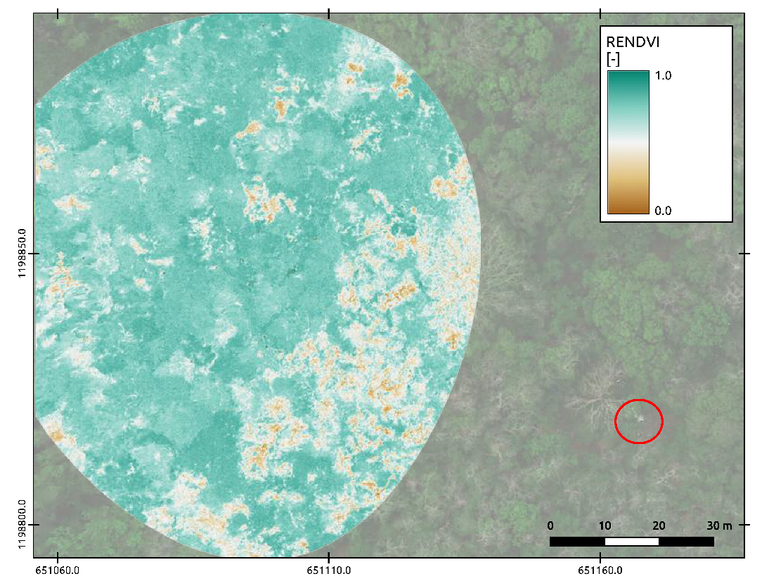
Figure 5.
Spatial distribution of the rededge based vegetation index (RENDVI) cropped for the footprint of the EC system. Red circle indicates the position of the EC system.
Figure 5.
Spatial distribution of the rededge based vegetation index (RENDVI) cropped for the footprint of the EC system. Red circle indicates the position of the EC system.

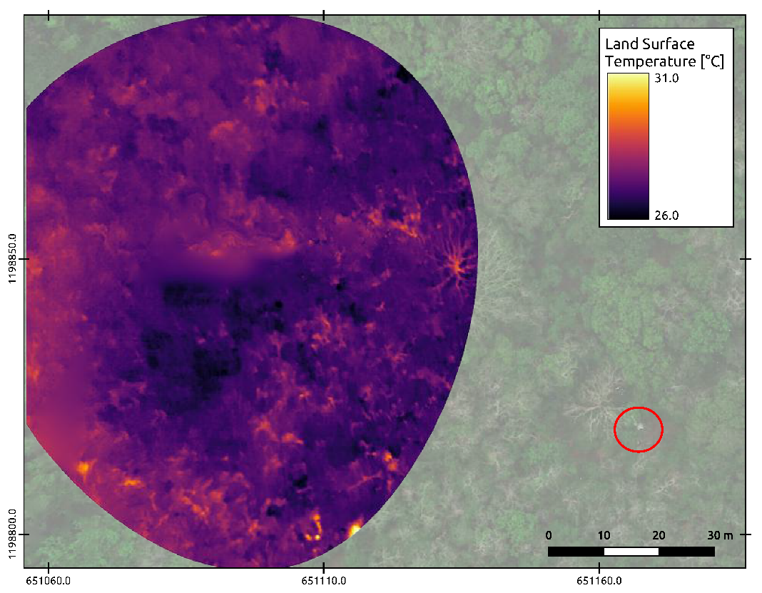
Figure 6.
Spatial distribution of the canopy surface temperature based on the TIR orthomosaic cropped for the footprint of the EC system. Red circle indicates the position of the EC system.
Figure 6.
Spatial distribution of the canopy surface temperature based on the TIR orthomosaic cropped for the footprint of the EC system. Red circle indicates the position of the EC system.

Figure 7.
RENDVI-LST triangle plot including dry and wet edges.

Figure 8.
Modeled latent heat flux cropped for the 10th and 20th percentiles of the EC system footprint representing 63% of the flux contribution. Red circle indicates the position of the EC system.
Figure 8.
Modeled latent heat flux cropped for the 10th and 20th percentiles of the EC system footprint representing 63% of the flux contribution. Red circle indicates the position of the EC system.


Table 1.
Specification of the Micasense RedEdge and FLIR TAU2 640 camera systems. GSD: ground sampling distance; HFOV: horizontal field Of view.
Table 1.
Specification of the Micasense RedEdge and FLIR TAU2 640 camera systems. GSD: ground sampling distance; HFOV: horizontal field Of view.
| Parameter | Micasense RedEdge | FLIR TAU2 640 |
|---|---|---|
| Dimensions [m] | 0.121 × 0.066 × 0.046 | 0.045 × 0.045 × 0.060 |
| Weight | 150 g | 95 g |
| Spectral bands | ||
| (Center wavelength and bandwidth per channel [nm]) | Blue 475 (20), green 560 (20), red 668 (10), red edge 717 (10), near IR 840 (40), narrow band | 7500–13,500, broad band |
| Resolution | 1280 × 980 pixels | 640 × 512 pixels |
| Focal length | 0.0055 m | 0.013 m |
| GSD at 100 m above ground | 0.07 m (per band) | 0.13 |
| Field of View | 47.2° HFOV | 45° × 37° 1.308 mr |
Table 2.
Acquired and used data within the Santa Rosa National Park Environmental Monitoring Super-Site.
Table 2.
Acquired and used data within the Santa Rosa National Park Environmental Monitoring Super-Site.
| Parameter | Sensor | Remarks |
|---|---|---|
| LST | UAV-FLIR TAU2 640 | Images were acquired at an altitude of 100 m above ground (canopy layer) |
| VIS-NIR | UAV-Micasense | Images were acquired at an altitude of 100 m above ground (canopy layer) |
| Kipp & Zonen CNR4 Net Radiometer | Net-radiation was measured every 10 min at the EC system | |
| G | HukseFlux HFP01SC | Soil heat flux was measured every 10 min within the footprint of the EC system |
| Decagon VP-3 | Air temperature was measured every 10 min at the EC system and within the EC footprint | |
| RH | Decagon VP-3 | Relative humidity was measured every 10 min at the EC system and within the EC footprint |
| E | Licor LI-7500DS & Gill Windmaster | Fluxes were measured at 10 Hz and integrated over a time span of 30 min and analyzed using Licor’s EddyPro software |
© 2020 by the authors. Licensee MDPI, Basel, Switzerland. This article is an open access article distributed under the terms and conditions of the Creative Commons Attribution (CC BY) license (http://creativecommons.org/licenses/by/4.0/).
Share and Cite
MDPI and ACS Style
Marzahn, P.; Flade, L.; Sanchez-Azofeifa, A. Spatial Estimation of the Latent Heat Flux in a Tropical Dry Forest by Using Unmanned Aerial Vehicles. Forests 2020, 11, 604. https://doi.org/10.3390/f11060604
AMA Style
Marzahn P, Flade L, Sanchez-Azofeifa A. Spatial Estimation of the Latent Heat Flux in a Tropical Dry Forest by Using Unmanned Aerial Vehicles. Forests. 2020; 11(6):604. https://doi.org/10.3390/f11060604
Chicago/Turabian StyleMarzahn, Philip, Linda Flade, and Arturo Sanchez-Azofeifa. 2020. "Spatial Estimation of the Latent Heat Flux in a Tropical Dry Forest by Using Unmanned Aerial Vehicles" Forests 11, no. 6: 604. https://doi.org/10.3390/f11060604
Note that from the first issue of 2016, this journal uses article numbers instead of page numbers. See further details here.