Integrating TimeSync Disturbance Detection and Repeat Forest Inventory to Predict Carbon Flux

1
United States Department of Agriculture Forest Service, Pacific Northwest Research Station, 3200 SW Jefferson Way, Corvallis, OR 97331, USA
2
Department of Forest Ecosystems & Society, Oregon State University, 321 Richardson Hall, Corvallis, OR 97331, USA
3
United States Department of Agriculture Forest Service, Rocky Mountain Research Station, 507 25th Street, Ogden, UT 84401, USA
*
Author to whom correspondence should be addressed.
Forests 2019, 10(11), 984; https://doi.org/10.3390/f10110984
Submission received: 2 October 2019
/
Revised: 30 October 2019
/
Accepted: 1 November 2019
/
Published: 5 November 2019
(This article belongs to the Special Issue Estimating change in forests: Merging Ground-, Photo-, and Space-Based Observations)
Abstract
:Understanding change in forest carbon (C) is important for devising strategies to reduce emissions of greenhouse gases. National forest inventories (NFIs) are important to meet international accounting goals, but data are often incomplete going back in time, and the amount of time between remeasurements can make attribution of C flux to specific events difficult. The long time series of Landsat imagery provides spatially comprehensive, consistent information that can be used to fill the gaps in ground measurements with predictive models. To evaluate such models, we relate Landsat spectral changes and disturbance interpretations directly to C flux measured on NFI plots and compare the performance of models with and without ground-measured predictor variables. The study was conducted in the forests of southwest Oregon State, USA, a region of diverse forest types, disturbances, and landowner management objectives. Plot data consisted of 676 NFI plots with remeasured individual tree data over a mean interval (time 1 to time 2) of 10.0 years. We calculated change in live aboveground woody carbon (AWC), including separate components of growth, mortality, and harvest. We interpreted radiometrically corrected annual Landsat images with the TimeSync (TS) tool for a 90 m × 90 m area over each plot. Spectral time series were divided into segments of similar trajectories and classified as disturbance, recovery, or stability segments, with type of disturbance identified. We calculated a variety of values and segment changes from tasseled cap angle and distance (TCA and TCD) as potential predictor variables of C flux. Multiple linear regression was used to model AWC and net change in AWC from the TS change metrics. The TS attribution of disturbance matched the plot measurements 89% of the time regarding whether fire or harvest had occurred or not. The primary disagreement was due to plots that had been partially cut, mostly in vigorous stands where the net change in AWC over the measurement was positive in spite of cutting. The plot-measured AWC at time 2 was 86.0 ± 78.7 Mg C ha−1 (mean and standard deviation), and the change in AWC across all plots was 3.5 ± 33 Mg C ha−1 year−1. The best model for AWC based solely on TS and other mapped variables had an R2 = 0.52 (RMSE = 54.6 Mg C ha−1); applying this model at two time periods to estimate net change in AWC resulted in an R2 = 0.25 (RMSE = 28.3 Mg ha−1) and a mean error of −5.4 Mg ha−1. The best model for AWC at time 2 using plot measurements at time 1 and TS variables had an R2 = 0.95 (RSME = 17.0 Mg ha−1). The model for net change in AWC using the same data was identical except that, because the variable being estimated was smaller in magnitude, the R2 = 0.73. All models performed better at estimating net change in AWC on TS-disturbed plots than on TS-undisturbed plots. The TS discrimination of disturbance between fire and harvest was an important variable in the models because the magnitude of spectral change from fire was greater for a given change in AWC. Regional models without plot-level predictors produced erroneous predictions of net change in AWC for some of the forest types. Our study suggests that, in spite of the simplicity of applying a single carbon model to multiple image dates, the approach can produce inaccurate estimates of C flux. Although models built with plot-level predictors are necessarily constrained to making predictions at plot locations, they show promise for providing accurate updates or back-calculations of C flux assessments.
1. Introduction
Given the accelerating effects of anthropogenic global warming [1], understanding the contributions of human land use to atmospheric carbon dioxide concentrations is useful for devising solutions. Forest ecosystems are important to terrestrial carbon cycling because most forests store more carbon (C) than other ecosystems and because those C stocks are dynamic [2]. Changes in the area of forest land use and mortality of live trees from natural disturbances, climatic stressors, forest product harvest, and growth of vegetation all affect C flux between forests and the atmosphere. Each of these drivers of C flux varies over time, complicating efforts to assess annual C flux nationally for 1990 and subsequent years, as many nations agreed to under the United Nations Framework Convention on Climate Change. As a result, substantial uncertainty remains on both the magnitude of fluxes in different vegetation types and the impact of harvest and natural disturbance [3,4].
Data are not always available to estimate C flux with the preferred approach under the Intergovernmental Panel on Climate Change (IPCC) standards for estimating C flux from forestlands [5], which puts the highest confidence in the extensive, statistically sound sampling done by national forest inventories (NFI). NFIs typically avoid model-based inference that may be subject to bias, and they rely on design-based or model-assisted inference that requires no assumptions about the relationship between sample measurements and ancillary data [6,7]. The effects of land-use change, management, disturbance, and growth are fully accounted for in repeated NFIs, even if they are not always analyzed explicitly. The NFI in the United States has evolved over time from a focus on regional timber supplies to a nationally consistent assessment of all forestlands that informs national C flux reporting [8,9,10,11]. However, reduced consistency and completeness prior to 2000 makes it impossible to make design-based inference on flux in 1990 in most parts of the country. In addition, the long (10+ years) remeasurement periods in the western U.S. makes attributing flux to specific economic, disturbance, or climatic events difficult. However, the rich plot-level data available on species composition, tree size, and growth and mortality rates can be used to inform models that extrapolate or project forest dynamics through time and space.
Landsat time series have proved useful for estimating vegetation density and disturbance and for developing models of forest carbon flux. The freely available Landsat archive has enabled the development and application of algorithms that produce radiometrically normalized and temporally smoothed time series of change for every pixel in an image (e.g., Kennedy et al. 2012; Zhu and Woodcock 2014). Furthermore, the visualization of spectral changes at the pixel level along with other spatial and image data (e.g., fire polygons, high-resolution photos) by trained analysts in tools like TimeSync (TS) [12] enable classification and interpretation of the nature of vegetation change captured in Landsat time series. While quite robust at detecting severe forest disturbances, questions remain concerning algorithm accuracy in different vegetation types and sensitivity to light- and moderate-severity disturbances [13,14]. In addition, large levels of tree cover tend to develop quickly after disturbance in productive vegetation types, which can saturate the Landsat signal, such that forest biomass and carbon continue to increase as stands mature, with little to no change in spectral signatures [15]. Nevertheless, the Landsat record can be used to estimate time since disturbances that originated after 1972 and can be combined with extensive information on forest density and change from NFIs to estimate flux at regional scales [16]. The time-series may also be used to estimate flux directly from the changes in spectral signature, which is the focus of this paper.
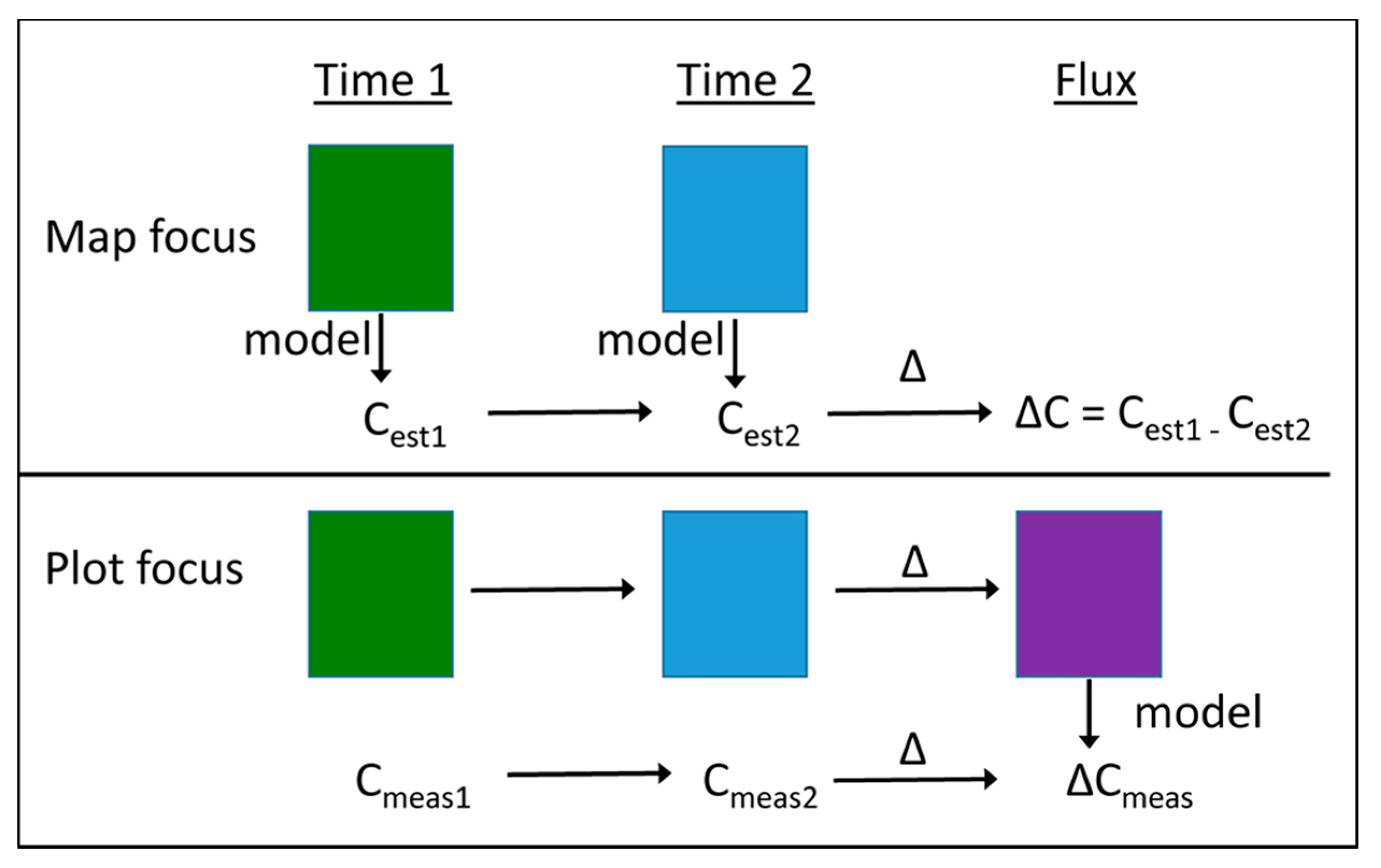
While most remote-sensing work in forests uses plots to inform maps, here we wanted to use remote sensing to inform changes on plots in order to take advantage of the rich composition and structure data available (Figure 1). Many applications of Landsat data to estimate forest C develop statistical models between sample plot C density and spectral characteristics at a point in time and apply the models to pixels across a region to generate maps of estimated C stocks. Frequently, C fluxes are estimated by applying the same model to Landsat imagery from a different point in time and then subtracting the estimates (Figure 1). The estimation of change by subtraction of modeled estimates of stocks has been referred to as the “indirect” approach, in contrast to the “direct” approach which models change in stocks from changes in spectral signatures [17]. The expectation that the direct approach should provide the most precise estimates of change by directly using the magnitudes and directions of the spectral changes in the time series is sometimes supported [18,19], but not always [17,20]. The objective of our study was to relate field-measured C flux to Landsat spectral changes interpreted with TS directly across a diverse, dynamic landscape as a proof-of-concept for subsequently updating or back-calculating field measurements with imagery. Specific objectives include: (1) compare TS detection of disturbance with plot-based measurements; (2) compare estimation of C flux from models that estimate C stocks using spatially comprehensive predictors to models that estimate C flux using plot-based measurements and TS change data; and (3) assess the ability of models to capture flux in different forest ecosystem types.
2. Methods
2.1. Study Area
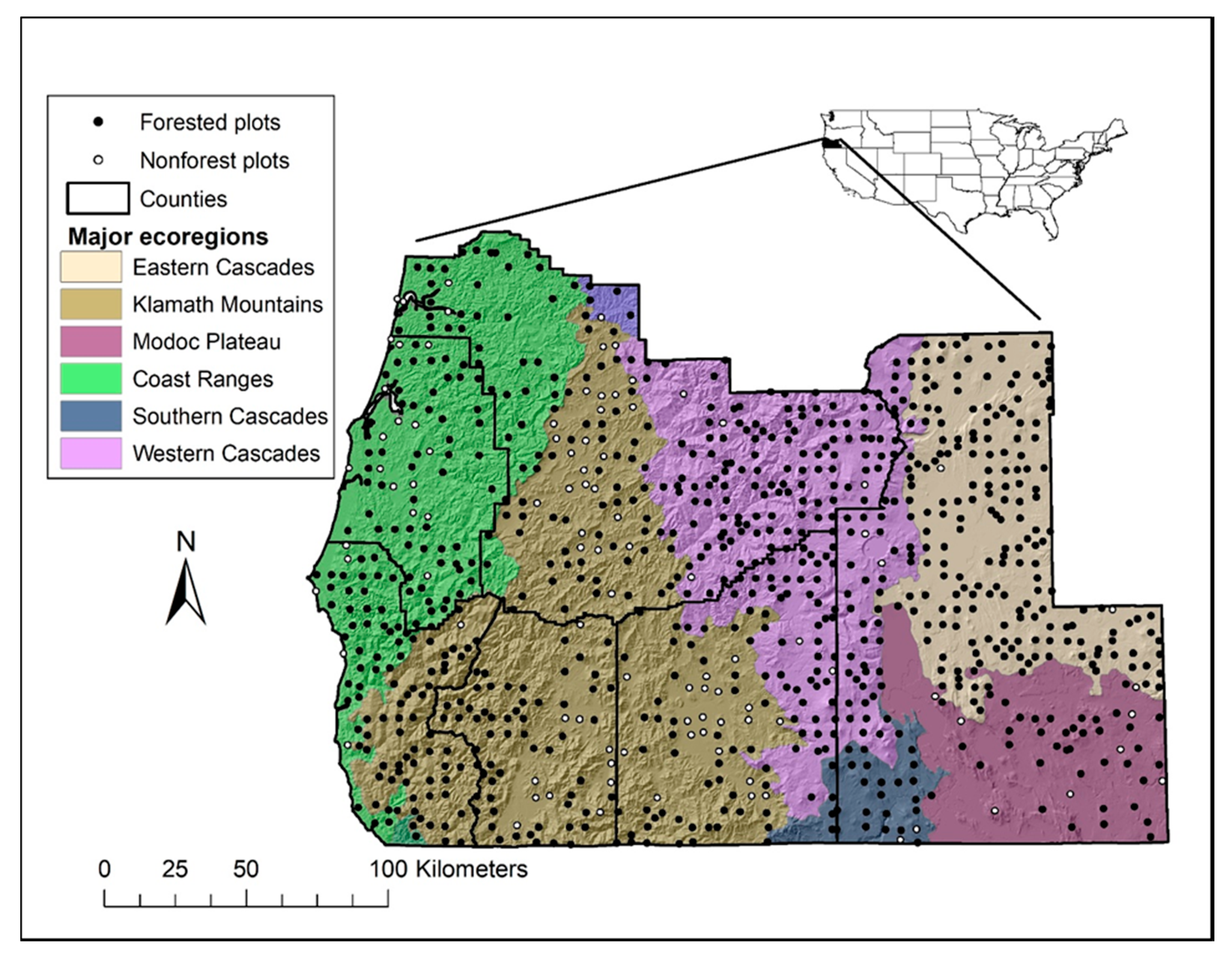
The study area included a wide range of vegetation conditions and management and disturbance histories in southwest Oregon, USA, that spanned six of Cleland et al.’s [21] ecoregion sections (Figure 2). The area was defined as most of the forested lands in six counties (Coos, Curry, Douglas, Jackson, Josephine, and Klamath) between 42.0° and 43.9° N latitude and 120.9° and 124.6° W longitude. Elevation ranges from 0 to 2800 m (933 ± 550 mean and standard deviation) and annual precipitation from 29 to 367 cm (130 ± 58 mean and standard deviation, based on Daymet) [22] (Supplemental Figure S1). Climax vegetation series range from western hemlock (Tsuga heterophylla) and tanoak (Lithocarpus densiflorus) in the Coast Ranges, to Douglas fir (Pseudotsuga menziesii) and Oregon white oak (Quercus garryana) in the interior valleys of the Klamath Mountains, to mountain hemlock (Tsuga mertensiana) in the higher elevations of the Western Cascades, to Ponderosa pine (Pinus ponderosa) and western juniper (Juniperus occidentalis) in the Eastern Cascades and Modoc Plateau [23]. The total land area is 4.9 million ha, of which 84% is forested (based on NFI) [24]. Of the forested lands, 41% is managed by the National Forest Systems (NFS), 17% by the Bureau of Land Management (BLM), 38% by private owners, and the remaining 4% by other federal, state, and local agencies (Supplemental Figure S2). Since the mid-1990s, federal management has emphasized protection and restoration of forest structural diversity through partial cutting, while private owners have tended to harvest more frequently and intensively [25]. Nine percent of the forestland in the area is in a protected status (e.g., wilderness, national park, or national monument). Forest fires are not uncommon; one of the largest in Oregon state recorded history occurred in the study area in 2002 (the Biscuit Fire, which covered 200,000 ha).
2.2. Plot Data
The ground-measured data used in this study were collected under two separate forest inventories: (1) the United States Department of Agriculture (USDA) Forest Service’s Forest Iinventory and Analysis (FIA) periodic inventory [26,27,28], and (2) the Pacific Northwest Region of the USDA Forest Service’s Current Vegetation Survey (CVS) inventory [29]. Both inventories used a probability-based sample design; the FIA sample consisted of a randomized systematic grid at a 5.47 km spacing on lands that were not managed by NFS or western Oregon BLM, while the CVS sample consisted of a systematic square grid at a 5.47 km spacing across NFS lands, and a denser grid at a 2.74 km spacing outside of designated Wilderness areas, providing a sample density of one plot per 3000 and 750 ha, respectively. A single, nationally consistent forest inventory approach, referred to as “annual FIA,” was instituted across all ownerships in Oregon starting in 2001 where the grid consisted of randomly selected, previously measured plots (where available) within 2400 ha hexagons [24]. Although western Oregon BLM lands also had a CVS-style inventory, remeasurement data were not available at the time this study was initiated, and their plot sample was not included in the selection criteria for annual FIA plots. Nevertheless, we expect that the selected inventories capture a broad range in vegetation conditions, disturbance types, and carbon trajectories to be useful for a proof-of-concept for this landscape. The FIA periodic inventory measured plots that qualified as forested (i.e., land areas ≥0.4 ha and >36 m wide that support or previously supported ≥10% tree canopy cover and were not primarily managed for a nonforest use). FIA plots were measured in the 1980s (1985–1988) and remeasured in the 1990s (1995–1999), for a mean remeasurement interval of 10 years. CVS plots were installed in 1993–1997 and remeasured 1997–2007, with a remeasurement period that ranged from 1–14 years with a mean of 7.1 years.
Plots from either inventory that were forested and measured twice, and were on the same grid intensity (one plot per 3000 ha, to ensure a balanced representation of vegetation conditions), were selected for analysis. In addition, only plots that had also been measured in annual FIA through 2007 were used, as these had been manually checked for accuracy of plot-based land-use and disturbance information for related studies. Furthermore, plot locations were never adjusted, so some plots straddled boundaries between different stands or land-use types. While this is not a problem for inventory estimation, it can be a problem for constructing models using imagery because different stands can have different reflectance characteristics and experience disturbance at different times. As a result, only plots where at least four-fifths of the plot area was in a single forested condition were used as a compromise between stronger signal fidelity and a reduced, biased sample size. Finally, 9% of the remaining CVS plots were excluded because the remeasurement occurred less than 5 years after plot installation, which was deemed too short a period to accurately reflect change in live tree biomass and shorter than any planned future inventory remeasurement cycle. These criteria resulted in 416 CVS plots and 260 periodic FIA plots being selected (n = 676). The mean and standard deviation of the remeasurement period for this set of plots was 10.0 ± 1.4 years.
The periodic FIA plot design consisted of five variable-radius points, while the CVS design consisted of nested fixed-radius subplots of different sizes around five points. This analysis focused on changes in the live tree forest component; calculations of tree biomass, and change components of growth, mortality, and harvest, were consistent among datasets. Estimates of aboveground live-tree woody biomass were based on regional FIA models of the sum of bole, bark, and branch biomass for each tree measurement. Bole biomass (ground to tip) was calculated from regional species-specific volume equations and wood densities [30]. Bark and branch biomass were calculated from regional species-specific equations selected from Means et al. [31] and documented in USDA Forest Service [32]. An expansion factor derived from the fixed-area plot size or the tree’s diameter and variable-radius prism factor (depending on tree selection method) was used to convert individual tree biomass to an area basis (Mg ha−1). We summed bole, bark, and branch estimates on each plot and multiplied by 0.5 for an estimate of above-ground live woody carbon (AWC). Net change in AWC between the first and second measurements (time 1 and time 2, respectively) was calculated by subtraction and referred to as ΔAWC. Changes in size and status of individual trees tracked on the plots was compiled into components of growth, mortality, and harvest. Additional information on data compilation can be found in Gray and Whittier [33] and Gray et al. [34]. We also included a few commonly available calculated variables from inventory plots as potential predictor variables (Table 1). The annual growth rate for each live tree at time 1 was available from prior measurements, increment cores, or modeling [35], from which an estimated increase in stand AWC due to growth was calculated (GROWMODEL). Stand age was estimated in the field as the average age of overstory dominant trees, based on increment cores. We estimated site productivity in terms of production of wood at culmination of mean annual increment (MAI, m3 ha−1 year−1) from measurements of site index trees (i.e., height and age) on each plot [36].
Disturbance codes were collected in the field on most plots or gleaned from written descriptions provided by field crews (disturbance coding was more complete and comprehensive during annual FIA measurements, which included coding prior disturbances that may have been described during the periodic or CVS inventories). Crews noted the type and timing of harvest or fire that occurred and also noted damage or mortality to live trees from animals, insects, disease, or weather. Plot-recorded disturbances were grouped for analysis into harvest, fire, fire and harvest, and other (including plots where crews coded that cutting occurred in the stand but none of the measured trees on the plot were cut). Plots that experienced both fire and cutting were subsequently grouped with harvest. Plant species composition observed in the field was used to classify plots to plant association using regional Forest Service guides [37,38,39]; we grouped these into plant association zones (PAZs) for analysis. Although most PAZs are named after conifer species, 15% of the plots in this study were dominated by hardwood tree species. Basic plot attributes summarized by PAZ are shown in Supplemental Table S1.
2.3. Remote-Sensed Data
The satellite data used to generate predictor variables of AWC change were created from annual Landsat time series of radiometrically normalized Landsat Thematic Mapper and Enhanced Thematic Mapper Plus images from 1984–2007 following method in Kennedy et al. 2010 [40]. The radiometrically normalized time series were then visually inspected at each inventory plot location using the TimeSync (TS) tool [12] to manually segment the time series between vertices of change in slope and classify segment types as disturbance, recovery, or stability, and, for segments that were disturbed, identify disturbance agents.
To model change in AWC (ΔAWC) with the aid of TS, we calculated the tasseled cap angle (TCA) from TC greenness and brightness described in Powell et al. [41] as TCA = arctan(TCG/TCB), and TC distance (TCD) as first described in Duane et al. [42], where TCD = (TCG2 + TCB2)½. In a similar study, Pflugmacher et al. [43] found TCA to be related to vegetation cover, useful in characterizing change in forest biomass, and TCD to be related to forest structure and composition, useful in characterizing current conditions. For each plot evaluated, we temporally smoothed the spectral data between segment vertices by fitting an ordinary least-squares linear regression on spectral values as a function of time. Starting with the first, segments were fitted in successive order to assure continuity (e.g., the fitted value from the end vertex of the first segment was used to fit the second segment). For abrupt disturbance segments, the fitted end vertex from the previous segment was used for that segment’s start vertex instead of the observed spectral value. Fitting was done independently for TCA and TCD.
Finally, for each field plot, we extracted the spectral values and time-series metrics associated with the 30 × 30 m Landsat pixel that contained the plot center. Because a 3 by 3 mean filter had been applied to all spatial data, the effective ground area sampled was 90 × 90 m around the plot center. The result was a series of segments for each 90 m area with annual reflectance values interpolated between the segment ends (vertices). Some of the change segments were attributed with the disturbances coded as delay, mechanical other, other non-disturbance, and stress and tended to be of low magnitude; these were grouped for analysis as “Other”.
TS segments, or portions thereof, were extracted for analysis based on the dates of plot measurement. For stable and recovery segments, the segments were truncated if necessary to coincide with the plot measurement years. For disturbance segments that coincided with the year of plot measurement, the plot disturbance codes and crew field notes were examined to determine whether to include the disturbance in the time series for the plot or not.
Predictor variables were calculated from the TS data to characterize the magnitude and duration of disturbance or recovery processes, based on those used by Pflugmacher et al. [44]. Disturbance-related variables were keyed to the greatest disturbance in the time series (in this case, between the plot measurement dates), determined as the disturbance segment with the greatest change in TCA values (Table 1). Other variables describe TCA and TCD values and trends prior to and following the greatest disturbance. Time series without disturbance were described by the current condition, current trend, and last monotonic trend variables.
2.4. Statistical Analyses
We compared the classification of disturbance types between the plot data and the TS analysis. Agreement rates of different groupings were calculated. The means and distributions of plot and TS change variables were generated to investigate the characteristics of discrepancies between the methods.
We used multiple linear regression analyses to explore the relationships between AWC at time 2 and ΔAWC between measurements (responses), and the plot- and TS-derived variables (predictors) as:
where Y is the estimated plot-level AWC (or ΔAWC) for each plot j, X is the value for each independent variable i for each plot j, and a and bi are coefficients estimated by the regression model.
Two types of analyses were done: (1) using only remotely sensed variables and (2) using remotely sensed variables and plot measurements at time 1, including net tree growth rates (net growth is growth of live trees minus mortality). The tree productivity variable MAI, although based on plot measurements, was also included in the first model because spatial models of MAI were available in the region [45]. MAI integrates climate, topography, and soils in a variable directly meaningful to live tree carbon flux, making those additional variables superfluous.
Prior to building regression models, we removed variables with similar information as determined by a correlation coefficient >0.5 with other predictor variables. We used stepwise model selection with a minimum p-value of 0.15 on each type of analysis. To avoid over-fitting, and because most of the models still had large numbers of variables (n > 10), we selected the model with the lowest value for Schwarz’ Bayesian information criterion [46]. Separate change-analysis models were run for TS-disturbed and -undisturbed plots since the relevant variable sets were different, and predicted values were combined to calculate overall model accuracy.
3. Results
3.1. Comparison of Plot- and TimeSync-Detected Disturbances
Disturbances were recorded in the field for the plot measurement intervals on 400 of the 676 plots used in the analysis (59%) and coded in the TS interpretations for 187 of the plots (28%). The largest category of field-recorded disturbance was the “Insect & Disease” group; while 10% of these were coded as “Stress” disturbance in TS, the majority (82%) did not have a TS disturbance (Table 2). Because the threshold for coding insect and disease damage to trees in the field did not require large levels of mortality, it is likely that, in most cases, there was only minor and/or gradual loss of canopy, which may not have been readily detectable in the TS imagery. The AWC that died on insect and disease plots not coded as disturbed by TS was 7.7 ± 2.0 Mg ha−1 (mean and 95% confidence interval; or 0.8 Mg ha−1 year−1), which was close to, yet significantly greater than (confidence interval outside the mean), the mortality on plots not coded for disturbance in the field (5.0 ± 0.95 Mg ha−1). While several plots were coded in the field as having had both fire and harvest occur during the measurement interval, TS coded those as one or the other.
When the analysis was constrained to the primary disturbances of fire and harvest, the plot and TS approaches agreed that 70% of the plots had not been affected, and that 19% of the plots were affected, for an overall agreement rate of 89% (Table 3). Of the nine plots coded by TS as fire or harvest but with nothing coded on plot, examination of field notes and National Agriculture Imagery Program aerial photographic imagery indicated that five locations had harvesting, and one had flood erosion, happen within 200 m of plot center.
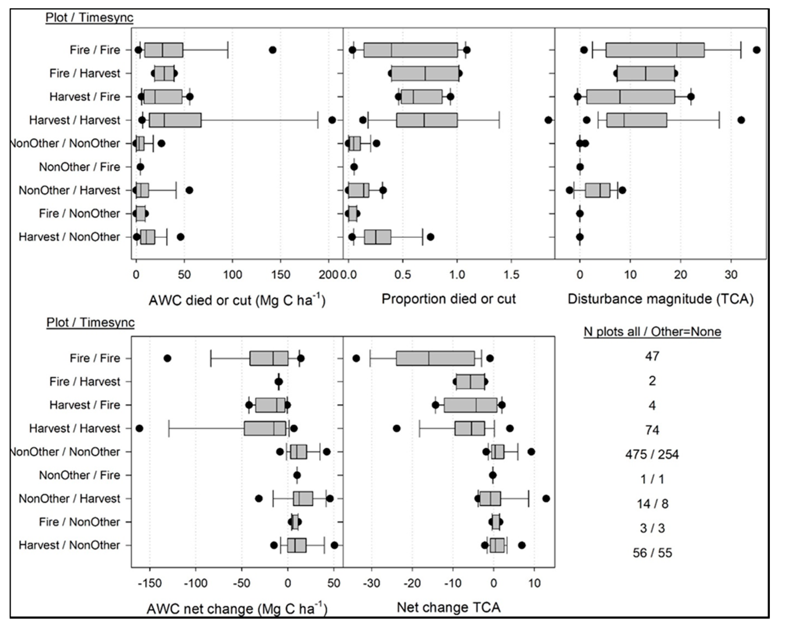
There were 55 plots with harvest coded in the field but with no disturbance recorded in TS. The AWC that was harvested or died was substantial on these plots, with a mean of 14.1 Mg ha−1, or 32% of AWC at time 1 (Table 3, Figure 3; category “Harvest/NonOther”). The type of harvest coded in the field on most of these plots was “light” partial harvest or precommercial thinning and represented 12.5% of the AWC cut on all plots. Overall, these were young vigorous stands, with positive ΔAWC and ΔTCA over the measurement period comparable to that of the undisturbed “NonOther/NonOther” plots (ΔAWC of 11.4 vs. 12.0 Mg ha−1 year−1 and ΔTCA of 1.1 vs. 1.7, respectively). Although the AWC that died or was cut was less on fire than on harvest plots, in absolute values as well as proportionally, the TCA response in terms of disturbance magnitude and net change was greater on fire than on harvest plots (Figure 3).
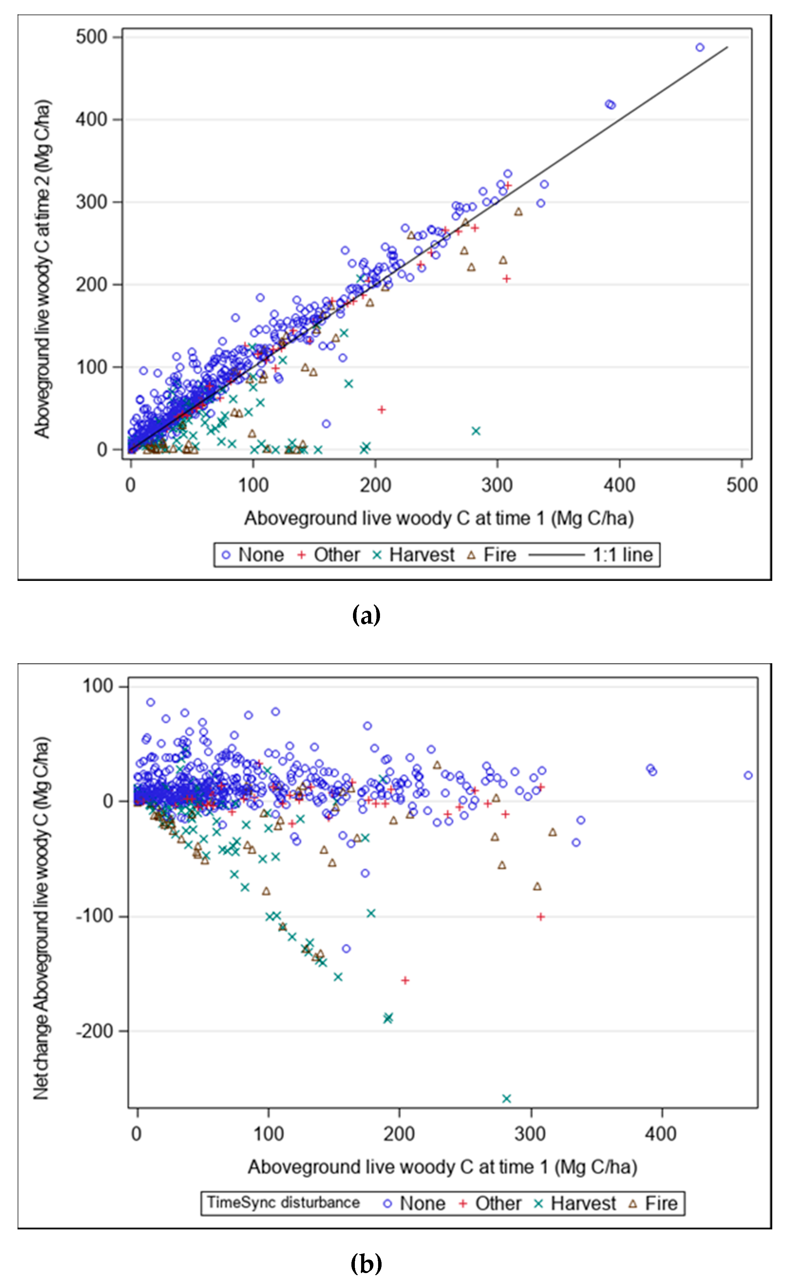
As would be expected, given that most plots were not disturbed, the majority of the plots fell close to a 1:1 line when comparing AWC at time 1 to AWC at time 2 (Figure 4a). In addition, many of the plots that were disturbed lost only modest amounts of AWC. The results appear more variable in terms of ΔAWC, however, with a wide range of net increases in undisturbed plots, particularly at lower values of AWC at time 1 (AWC1), and a range of losses attributed to disturbance (Figure 4b). Across all plots, AWC at time 2 was 86.0 ± 78.7 Mg ha−1 and ΔAWC was 3.5 ± 33 Mg ha−1 year−1 (Supplemental Table S1).
3.2. Modeling Change in Live-Tree Carbon
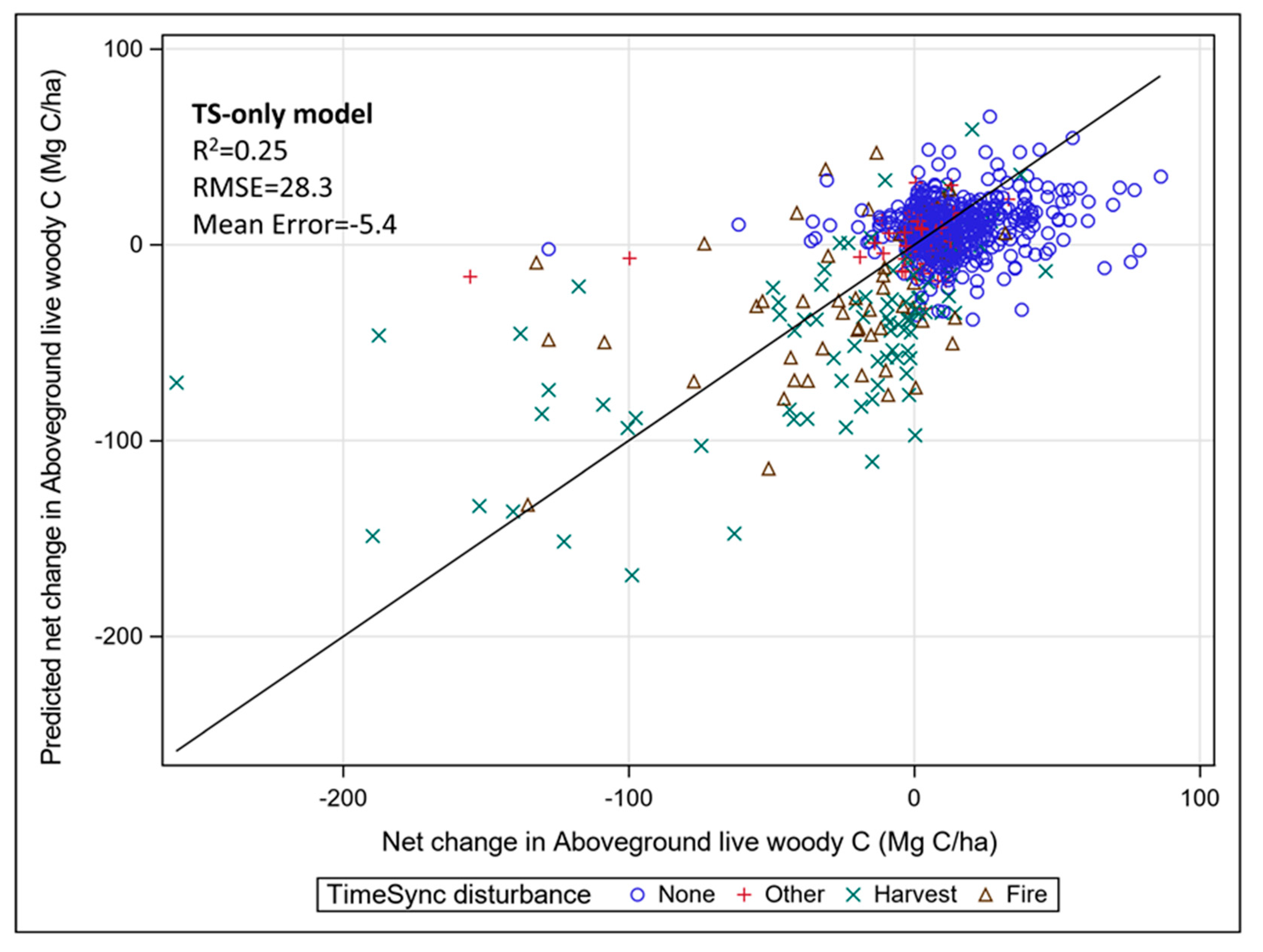
The selected model using TS variables and MAI to predict AWC at time 2 included predicted site productivity (MAI), spectral indices at time 2 (CCTCA2 and CCTCD2), the magnitude of increases during the remeasurement period (TRMAG_A), and the duration of declines and increases (TDDUR_D, TRDUR_A) (Supplemental Table S2). The R2 equaled 0.53, with an RMSE of 54.3 Mg C ha−1. The influence of MAI on the model was substantial; the interquartile range in MAI of 5.6 equaled an effect size of 27.0 Mg ha−1 with the TS variables held constant, which was 31% of the mean AWC of 86.0 Mg ha−1. The accuracy of predictions varied by PAZ, with under-prediction of AWC suggested for the Pacific silver fir (ABAM) zone and over-prediction for the Ponderosa pine, Douglas fir, and Oregon white oak (PIPO, PSME, and QUGA) zone plots (Supplemental Figure S3). The model was applied to the TS values for time 1, and the time 1 predictions were subtracted from the time 2 predictions to estimate ΔAWC. The R2 for the predictions of ΔAWC was 0.25 with an RMSE of 28.3 Mg C ha−1 year−1 (Figure 5). Error in the estimated net change was an issue because it was based on subtraction of two predictions; estimates of ΔAWC were, on average, 5.4 Mg C ha−1 less than measured change (−1.9 vs. 3.5 Mg C ha−1 year−1).
The selected model using TS variables and plot data from time 1 to predict AWC at time 2 for undisturbed plots included the variables AWC at time 1 (and a squared term), site productivity (MAI), modeled net growth to time 2 (GROWMODEL), spectral index at time 1 and magnitude of declines between measurements (CCTCA1 and TDMAG_D), and the plot remeasurement period (REMPER) (Supplemental Table S3a). The R2 for AWC at time 2 was 0.97 with an RMSE of 13.0 Mg C ha−1. The best model for the disturbed plots included the variables AWC at time 1, AWC at time 1 for plots disturbed by harvest (GDAGT_HARV * AWC1), site productivity (MAI), spectral index after disturbance (ADVAL_A), and different metrics of changes in spectral index between measurements (CHGTCA, ADREC_A, TRROC_A) (Supplemental Table S3b). The importance of the harvest indicator term in the model likely is due to the greater change in TCA on fire plots for a given loss in AWC than on harvested plots (Supplemental Figure S5). The R2 for AWC at time 2 on disturbed plots was 0.88, with an RMSE of 25.3 Mg C ha−1. For the combined predictions of disturbed and undisturbed plots, the R2 = 0.95 with an RMSE of 17.0 Mg C ha−1 year−1 and a mean error of 0.
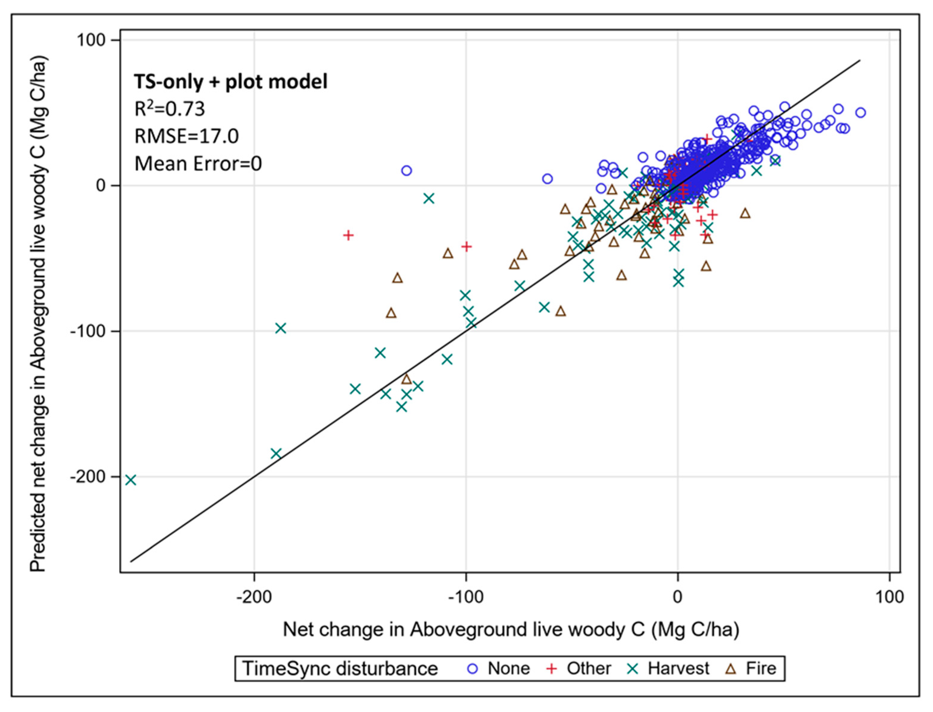
The models using all TS and time 1 plot data to estimate ΔAWC were almost identical to those that estimated AWC at time 2, with a few important differences. Because AWC1 was an independent variable in the model, AWC2 and ΔAWC are simply different expressions of the same relationship, so the parameters for the independent variables were the same, except for the intercept and AWC1 (compare Supplemental Tables S4 and S3). The RMSEs of the AWC2 and ΔAWC models were identical as well. However, the R2 differed because the magnitudes of the values being estimated were quite different. The R2 for the undisturbed, disturbed, and combined models for ΔAWC were 0.48, 0.70, and 0.73, respectively (Figure 6). The model for undisturbed plots tended to under-estimate change in AWC for the JUOC, PICO, and TSME PAZs and over-estimate for the ABAM PAZ, while the model for disturbed plots tended to not vary much by PAZ (Supplemental Figure S4).
4. Discussion
4.1. Disturbance Detection
Detection of disturbance with TS agreed with plot-based measurements for discrete, typically severe events of harvest or fire 89% of the time. The analyst-based classification of TS segments into fire versus harvest was also accurate, which was important for modeling C flux. The lack of greater agreement between methods was because 43% of the plots that were identified as partially harvested (thinned) or precommercially thinned in the field were coded as undisturbed in TS. Although a substantial amount of the AWC present at time 1 was cut on the missed plots (32%, or 14.1 Mg ha−1), this type of harvest in this region tends to primarily remove low-stature trees, with minor impact on live tree canopy and some increase in shadow, but likely little newly exposed soil visible in imagery. This TS-missed harvest represented 12.5% of the AWC cut across all plots, suggesting that other sources of information might be needed to accurately estimate harvest in regions where thinning from below is common. Despite working with new installation data (not remeasurements), Schroeder et al. [14] also found the greatest agreement between Landsat time-series and NFI field data on plots with mortality or removal of overstory trees.
Detection of light-severity and chronic disturbance and agreement between methods was more problematic. One of the difficulties, ecologically as well as for remote sensing, is distinguishing between a disturbance and “normal” background tree mortality. While the NFI field protocol sets a threshold of “mortality or damage to 25% of all trees in a stand or 50% of an individual species’ count”, the overall impact and visibility of the event in imagery will depend on the spatial distribution of effects, the size classes of trees affected, and the species composition of the stand. A large number of plots coded with insect and disease disturbance in the field, but nothing in TS is likely because the threshold includes damage to live trees short of mortality; indeed, the AWC of mortality trees on these plots was not much greater than on undisturbed plots. The difficulty of defining disturbance at the low-intensity end will always lead to these kinds of discrepancies, but for our study, at least the effect on modeling changes in AWC was negligible. Long Landsat time-series can be sensitive to subtle changes in canopy cover, however, and is an active area of research [47].
Despite the utility of the manually interpreted TS determinations of disturbance type for analysis and modeling, the required effort restricts its application to a relatively small number of plots or points. However, the manually interpreted points can be used to train a much larger set of points with multispectral change indices or patch shape metrics to estimate disturbance type across a much larger area or set of plots [48,49].
4.2. Modeling C Stocks and Stock Change with Only Spatial Predictors
The fit for the model of AWC stocks using the TS status and trend information up to the plot measurement was not very strong (R2 = 0.53), and it was substantially weaker than that found in a similar study by Pflugmacher et al. [44] conducted in eastern Oregon (R2 = 0.80). A likely reason for this is the greater variety of forest types and disturbance regimes in our study area. The spectral signatures at the time of plot measurement were highly influential in the model of AWC stocks, but the TS trend variables for the time prior to measurement were also important to the model, as found in Pflugmacher et al. [44]. The estimate of forest productivity (MAI) was important in the model and improved estimates of AWC for different types of forests with similar canopy characteristics and TS variables. Broader availability of spatially modeled estimates of site productivity (e.g., Latta et al. [45]), which integrate climate, soil, and topography into a meaningful metric for estimating forest biomass, could prove useful for other C modeling efforts.
The indirect estimate of net change in AWC (ΔAWC) derived from subtracting estimates of AWC stocks at time 1 and time 2 behaved quite poorly, with R2 = 0.25 and RMSE of 28.3 Mg ha−1 year−1, eight times the actual mean change in AWC of 3.5 Mg ha−1 year−1. The indirect estimation of ΔAWC also resulted in substantial mean error (−5.4 Mg ha−1 year−1). Although the model for AWC at time 2 built from plot data and TS was unbiased, there is no assurance that applying the same model to TS values for time 1 and subtracting the estimates would be unbiased. Studies that estimate changes in disturbed areas (e.g., Tao et al. [50]) may be less prone to error than those that estimate change in all forests, given the greater sensitivity of Landsat change detection to disturbance over growth (e.g., Battles et al. [51]). Of course, if disturbed forests are systematically different in biomass density than the “average” forests the Landsat-based model represents, estimates of sources and sinks of C will be biased [52].
Models that predict change directly tend to be more accurate than those that predict change indirectly [18,53,54], but the flexibility of applying a single model to multiple image dates with the indirect method is often thought to outweigh the problems (e.g., Powell et al. [55]). In many cases, ground measurements of change are not available, and indirect estimation of change is the only option (e.g., Andersen et al. [56]). In contrast, some applications of remote-sensing change detection attempt to improve the precision of NFI estimates from a complete set of remeasured plots and high-precision sensing (e.g., lidar). Indirect estimation is more precise in some cases, particularly when separate models are constructed relating biomass and imagery for each time period [17,20], but this is not always the case (e.g., Massey et al. [19]).
4.3. Modeling C Flux with Plot and Spatial Predictors
The fit for the models using plot measurements at time 1 and TS variables to estimate AWC at time 2 were quite good, with R2 = 0.97 and 0.88 for the undisturbed and disturbed plots, respectively, or 0.95 overall. Spectral change was important for both models, but change in TCD was most useful for undisturbed plots, while change in TCA was better for disturbed plots. This could be expected since TCA describes gradients of percent vegetation cover, while TCD is sensitive to vegetation structure and composition [43]. AWC at time 1, MAI, modeled net growth, and the remeasurement period were all important plot-level variables in the undisturbed model. Growth did not enter into the disturbed model, indicating that the net change was dominated by disturbance and the primary plot variable of importance was AWC at time 1. The additional inclusion of the harvest indicator-AWC1 interaction term reflects the substantial difference in spectral response between harvested and burned areas seen in other studies (e.g., Cohen et al. [57]), justifying the additional effort in classifying TS-detected disturbance types.
The models estimating ΔAWC using plot measurements at time 1 and TS variables were essentially identical to those predicting AWC at time 2 from plot measurements at time 1 and TS variables, since ΔAWC is simply the difference of the two. However, because the mean value of ΔAWC was much smaller than the mean value of AWC at time 2 (3.5 vs. 86.0 Mg ha−1 year−1, respectively), the R2 statistic was worse (0.73 vs. 0.95, respectively), even though the RMSE was the same (17.0 Mg ha−1 year−1). As a result, the RMSE was almost five times the mean ΔAWC being estimated.
4.4. Effect of Ecosystem Type
The ability of models to estimate C stocks or change for the large variation in vegetation types in the study area differed. The model based solely on TS and measurements at time 2 did fairly well with the most abundant vegetation types (western hemlock and tanoak climax zones), but it had substantial over-prediction for some of the vegetation types (Ponderosa pine and Douglas-fir climax zones), which usually attain high levels of canopy cover but nonetheless are less productive and biomass-dense than the most abundant types in the area. The plot-based models had fewer systematic errors by vegetation type, with the disturbed model being quite accurate across all types and the undisturbed model under-estimating ΔAWC for some of the vegetation types that often have sparse canopy cover (juniper, lodgepole pine, and mountain hemlock climax zones). Many studies focus on a single Landsat scene or specific vegetation types [58,59] or develop separate models for different vegetation types [42,60]. We specifically selected our study area to maximize the diversity of vegetation types, but developing models over a larger region could provide sufficient sample size for building separate models for different forest groups. Mapping applications that cannot include ground measurements as independent variables could use modeled vegetation type as predictors instead (e.g., Henderson et al. [61]). The use of ensembles of time-series algorithms to predict disturbance effects may be a practical approach to combining their differential abilities to quantify different disturbances (or lack thereof) in different vegetation types (e.g., Cohen et al. [13], Healey et al. [62]; but see Saxena et al. [63]).
4.5. Implications for Improving Carbon Assessments
Design-based estimates of forest C flux from remeasured NFI plots provide unbiased, accurate values that are routinely used to ground-truth remote-sensing models and validate landscape-level estimates. The confidence in an estimate for a particular land area (i.e., precision) increases with the number of NFI sample plots. For map-based estimates of C flux from Landsat time-series, models that estimate the different types of changes on the landscape without bias are desirable. Our study found that indirect estimation of C flux by subtracting estimates from a single model of C stocks applied to multitemporal imagery produced poor estimates overall and for some vegetation types in particular. Direct estimation of C flux from Landsat change metrics was more accurate than subtracting two estimates of stocks.
One of the difficulties with assessing C flux and the impact of discrete events with NFI data is that the field-based estimates are essentially a net change between two points in time. It is common for NFIs to estimate components of growth, mortality, and harvest for individually tracked live trees between measurements, although specialized field measurements that visit NFI plots soon after a large disturbance can better quantify immediate effects (e.g., Eskelson and Monleon [64]). These data could be combined with remotely sensed metrics of disturbance severity and vegetation regrowth to model plot-level components of change in live-tree AWC across the population of NFI plots.
A related difficulty with standard NFI-based assessments, particularly in the western U.S. where one-tenth of the plots are measured in spatially balanced panels over a ten-year cycle, is that most estimates of C flux are averages over substantial periods (e.g., a full remeasurement of all plots in an area would span 20 years). In our study, many of the plots within the footprint of the 200,000 ha Biscuit Fire of 2002 were remeasured before the fire so could not be used to characterize it. While it is possible to identify affected plots and make design-based estimates for specific fires or specific years (e.g., Figure 4.7 in Christensen et al. [65]), the sample size for anything but the largest events will be low until measurements accumulate over sufficient years to reflect that event. Using the larger population of NFI plots and associated remote-sensing to improve estimates of specific mapped areas of interest (often referred to as the “small area estimation” problem) is an active area of research (e.g., Mauro et al. [66]).
We modeled changes in live tree C in this study, which makes up the majority (~70%) of aboveground C pools in our region, but is not always the C pool most affected by disturbance. Models of forest dynamics built with remote sensing are primarily sensitive to changes in live canopy cover, and trees in particular. Many disturbances like fire, or insects and disease, may have modest impacts on overstory live tree cover but substantial effects on understory trees and plants, organic soil layers, and dead wood pools. Even when severe disturbances kill most of the live trees, most of the C stays on site for years or decades as dead wood [67] and can be missed or purposely excluded from estimates of C emissions (e.g., Garcia et al. [68]).
Landsat has been useful in distinguishing young, mature, and old-growth stands, even in regions where forest canopies are dense and the signal saturates [69]. However, for areas such as our study area, where C flux is dominated by growth in undisturbed stands, there will rarely be enough response in the signal over even a ten-year period to reflect growth [51]. Application of technologies that can measure change in tree height, like Lidar or 3-D NAIP could improve this ability, but are currently limited in extent. Researchers commonly rely on a variety of models to estimate live tree growth and changes in other C pools not captured well by the imagery. Models based on physiological processes, state-transition matrices, or forest growth-and-yield can be constrained to match measurements on NFI plots and used to map forest dynamics over time [16,70,71,72]. Nevertheless, even models that estimate similar levels of C uptake often disagree on the importance of different environmental drivers, making forecasting or back-casting problematic [73].
Our use of extrapolated live tree growth rates in this study greatly improved our ability to estimate C flux of undisturbed stands. The utility of this extrapolation undoubtedly degrades quickly as the time interval increases. Nevertheless, much of the value of this growth estimate is probably based on its specificity to the stand of interest rather than a model-derived mean. Modeling C flux of individual plots through time can utilize a number of high-quality predictor variables not available to spatial models that must rely on more generalized predictors. Nevertheless, predicting AWC for a location prior to a severe disturbance would need to either rely on a statistical mean based on the remote sensing signature, or additional interpretation (e.g., stereoscopic photo-interpretation). The combination of Landsat change metrics and plot data have the potential to provide updated NFI estimates where the model error is a minor component of the overall error [60].
5. Conclusions
We found that using remotely sensed change detection to predict change in live tree carbon in a diverse forested landscape was more accurate when modeled with field-measured predictors at individual NFI plots rather than with mapped predictors available across the landscape. While this limits predictions to those plot locations, it may result in better estimates of C flux than statistical estimates using remote sensing, which have difficulty representing C accumulation from growth in closed-canopy forests. Future applications of the model predictions at NFI plots could be combined with the inventory sample design to provide estimates of C flux for the 1990 baseline year or updates to the most recent year of Landsat measurement.
Supplementary Materials
The supplementary materials are available online at https://www.mdpi.com/1999-4907/10/11/984/s1.
Author Contributions
Conceptualization, A.N.G. and W.B.C.; Methodology, A.N.G., W.B.C. and Z.Y.; Validation, A.N.G., W.B.C. and E.P.; Formal Analysis, A.N.G. and Z.Y.; Investigation, W.B.C. and E.P.; Data Curation, A.N.G., W.B.C. and Z.Y.; Writing—Original Draft Preparation, A.N.G.; Writing—Review & Editing, A.N.G. and W.B.C.; Visualization, A.N.G.
Acknowledgments
Funding was provided by the USDA Forest Service Pacific Northwest Research Station. Thom Whittier assisted with initial data compilation for related studies. FIA and CVS field crews collected the field data in often-challenging conditions. National Forest Pacific Northwest Region managed and provided the CVS data.
Conflicts of Interest
Any use of trade, firm, or product names is for descriptive purposes only and does not imply endorsement by the U.S. Government.
References
- Hoegh-Guldberg, O.; Jacob, D.; Taylor, M.; Bindi, M.; Brown, S.; Camilloni, I.; Diedhiou, A.; Djalante, R.; Ebi, K.L.; Engelbrecht, F.; et al. Impacts of 1.5 °C Global Warming on Natural and Human Systems. In Global Warming of 1.5 °C. An IPCC Special Report on the Impacts of Global Warming of 1.5 °C above Pre-Industrial Levels and Related Global Greenhouse Gas Emission Pathways, in the Context of Strengthening the Global Response to the Threat of Climate Change, Sustainable Development, and Efforts to Eradicate Poverty; Intergovernmental Panel on Climate Change: Geneva, Switzerland, 2018. [Google Scholar]
- McKinley, D.C.; Ryan, M.G.; Birdsey, R.A.; Giardina, C.P.; Harmon, M.E.; Heath, L.S.; Houghton, R.A.; Jackson, R.B.; Morrison, J.F.; Murray, B.C.; et al. A synthesis of current knowledge on forests and carbon storage in the United States. Ecol. Appl. 2011, 21, 1902–1924. [Google Scholar] [CrossRef] [PubMed] [Green Version]
- Hayes, D.J.; Turner, D.P.; Stinson, G.; McGuire, A.D.; Wei, Y.; West, T.O.; Heath, L.S.; de Jong, B.; McConkey, B.G.; Birdsey, R.A.; et al. Reconciling estimates of the contemporary North American carbon balance among terrestrial biosphere models, atmospheric inversions, and a new approach for estimating net ecosystem exchange from inventory-based data. Glob. Chang. Biol. 2012, 18, 1282–1299. [Google Scholar] [CrossRef]
- Pan, Y.D.; Birdsey, R.A.; Fang, J.Y.; Houghton, R.; Kauppi, P.E.; Kurz, W.A.; Phillips, O.L.; Shvidenko, A.; Lewis, S.L.; Canadell, J.G.; et al. A large and persistent carbon sink in the world’s forests. Science 2011, 333, 988–993. [Google Scholar] [CrossRef] [PubMed]
- IPCC. 2013 Revised Supplementary Methods and Good Practice Guidance Arising from the Kyoto Protocol; Hiraishi, T., Krug, T., Tanabe, K., Srivastava, N., Baasansuren, J., Fukuda, M., Troxler, T.G., Eds.; IPCC: Geneva, Switzerland, 2014. [Google Scholar]
- Bechtold, W.A.; Patterson, P.L. The Enhanced Forest Inventory and Analysis Program-National Sampling Design and Estimation Procedures; USDA Forest Service, Southern Research Station: Asheville, NC, USA, 2005; p. 85.
- Kangas, A.; Maltamo, M. Forest Inventory: Methodology and Applications; Springer: Dordrecht, The Netherlands, 2006; p. 362. [Google Scholar]
- Gillespie, A.J.R. Rationale for a national annual forest inventory program. J. For. 1999, 97, 16–20. [Google Scholar]
- Heath, L.S.; Smith, J.E.; Woodall, C.W.; Azuma, D.; Waddell, K.L. Carbon stocks on forestland of the United States, with emphasis on USDA Forest Service ownership. Ecosphere 2011, 2, 1–21. [Google Scholar] [CrossRef]
- U.S. Environmental Protection Agency. Inventory of U.S. Greenhouse Gas Emissions and Sinks: 1990–2016; Environmental Protection Agency, Office of Atmospheric Programs: Washington, DC, USA, 2018; p. 655.
- Woodall, C.W.; Coulston, J.W.; Domke, G.M.; Walters, B.F.; Wear, D.N.; Smith, J.E.; Andersen, H.-E.; Clough, B.J.; Cohen, W.B.; Griffith, D.M.; et al. The U.S. Forest Carbon Accounting Framework: Stocks and Stock Change, 1990–2016; U.S. Department of Agriculture, Forest Service, Northern Research Station: Newtown Square, PA, USA, 2015; p. 49.
- Cohen, W.B.; Yang, Z.G.; Kennedy, R. Detecting trends in forest disturbance and recovery using yearly Landsat time series: 2. TimeSync-Tools for calibration and validation. Remote Sens. Environ. 2010, 114, 2911–2924. [Google Scholar] [CrossRef]
- Cohen, W.B.; Healey, S.P.; Yang, Z.; Stehman, S.V.; Brewer, C.K.; Brooks, E.B.; Gorelick, N.; Huang, C.; Hughes, M.J.; Kennedy, R.E.; et al. How similar are forest disturbance maps derived from different landsat time series algorithms? Forests 2017, 8, 98. [Google Scholar] [CrossRef]
- Schroeder, T.A.; Healey, S.P.; Moisen, G.G.; Frescino, T.S.; Cohen, W.B.; Huang, C.; Kennedy, R.E.; Yang, Z. Improving estimates of forest disturbance by combining observations from Landsat time series with U.S. forest service forest inventory and analysis data. Remote Sens. Environ. 2014, 154, 61–73. [Google Scholar] [CrossRef]
- Turner, D.P.; Cohen, W.B.; Kennedy, R.E.; Fassnacht, K.S.; Briggs, J.M. Relationships between leaf area index and Landsat TM spectral vegetation indices across three temperate zone sites. Remote Sens. Environ. 1999, 70, 52–68. [Google Scholar] [CrossRef]
- Turner, D.P.; Ritts, W.D.; Kennedy, R.E.; Gray, A.N.; Yang, Z. Regional carbon cycle responses to 25 years of variation in climate and disturbance in the US Pacific Northwest. Reg. Environ. Chang. 2016, 16, 2345–2355. [Google Scholar] [CrossRef]
- McRoberts, R.E.; Næsset, E.; Gobakken, T.; Bollandsås, O.M. Indirect and direct estimation of forest biomass change using forest inventory and airborne laser scanning data. Remote Sens. Environ. 2015, 164, 36–42. [Google Scholar] [CrossRef]
- Healey, S.P.; Yang, Z.; Cohen, W.B.; Pierce, D.J. Application of two regression-based methods to estimate the effects of partial harvest on forest structure using Landsat data. Remote Sens. Environ. 2006, 101, 115–126. [Google Scholar] [CrossRef]
- Massey, A.; Mandallaz, D. Design-based regression estimation of net change for forest inventories. Can. J. For. Res. 2015, 45, 1775–1784. [Google Scholar] [CrossRef]
- Bollandsås, O.M.; Ene, L.T.; Gobakken, T.; Næsset, E. Estimation of biomass change in montane forests in Norway along a 1200 km latitudinal gradient using airborne laser scanning: A comparison of direct and indirect prediction of change under a model-based inferential approach. Scand. J. For. Res. 2018, 33, 155–165. [Google Scholar] [CrossRef]
- Cleland, D.T.; Freeouf, J.A.; Keys, J.E., Jr.; Nowacki, G.J.; Carpenter, C.A.; McNab, W.H. Ecological Subregions: Sections and Subsections for the Conterminous United States; USDA Forest Service: Washington, DC, USA, 2007.
- Thornton, P.E.; Running, S.W.; White, M.A. Generating surfaces of daily meteorological variables over large regions of complex terrain. J. Hydrol. 1997, 190, 214–251. [Google Scholar] [CrossRef] [Green Version]
- Franklin, J.F.; Dyrness, C.T. Natural Vegetation of Oregon and Washington; USDA Forest Service Pacific Northwest Research Station: Portland, OR, USA, 1973; p. 417.
- Palmer, M.; Kuegler, O.; Christensen, G. Oregon’s Forest Resources, 2006–2015: Ten-Year Forest Inventory and Analysis Report; USDA Forest Service, Pacific Northwest Research Station: Portland, OR, USA, 2018; p. 54.
- Davis, R.J.; Ohmann, J.L.; Kennedy, R.E.; Cohen, W.B.; Gregory, M.J.; Yang, Z.; Roberts, H.M.; Gray, A.N.; Spies, T.A. Northwest Forest Plan-The First 20 Years (1994–2013): Status and Trends of Late-Successional and Old-Growth Forests; U.S. Department of Agriculture, Forest Service, Pacific Northwest Research Station: Portland, OR, USA, 2015; p. 112.
- Azuma, D.L.; Bednar, L.F.; Hiserote, B.A.; Veneklase, C.A. Timber Resource Statistics for Western Oregon, 1997; USDA Forest Service Pacific Northwest Research Station: Portland, OR, USA, 2004; p. 120.
- Azuma, D.L.; Dunham, P.A.; Hiserote, B.A.; Veneklase, C.A. Timber Resource Statistics for Eastern Oregon, 1999; USDA Forest Service Pacific Northwest Research Station: Portland, OR, USA, 2004; p. 42.
- Azuma, D.L.; Hiserote, B.A.; Dunham, P.A. The Western Juniper Resource of Eastern Oregon; USDA Forest Service Pacific Northwest Research Station: Portland, OR, USA, 2005; p. 18.
- Max, T.A.; Schreuder, H.T.; Hazard, J.W.; Oswald, D.D.; Teply, J.; Alegria, J. The Pacific Northwest Region Vegetation and Inventory Monitoring System; USDA Forest Service, Pacific Northwest Research Station: Portland, OR, USA, 1996; p. 22.
- USDA Forest Service. FIA Volume Equation Documentation Updated on 9-19-2014; USDA Forest Service: Portland, OR, USA, 2014; p. 57.
- Means, J.E.; Hansen, H.A.; Koerper, G.J.; Alaback, P.B.; Klopsch, M.W. Software for Computing Plant Biomass--BIOPAK Users Guide; USDA Forest Service Pacific Northwest Forest and Range Experiment Station: Portland, OR, USA, 1994; p. 184.
- USDA Forest Service. Regional Biomass Equations Used by FIA to Estimate Bole, Bark, and Branches; Updated 09-19-2014; USDA Forest Service: Portland, OR, USA, 2014; p. 23.
- Gray, A.N.; Whittier, T.R. Carbon stocks and changes on Pacific Northwest national forests and the role of disturbance, management, and growth. For. Ecol. Manag. 2014, 328, 167–178. [Google Scholar] [CrossRef]
- Gray, A.N.; Whittier, T.R.; Azuma, D.L. Estimation of above-ground forest carbon flux in oregon: Adding components of change to stock-difference assessments. For. Sci. 2014, 60, 317–326. [Google Scholar] [CrossRef]
- Waddell, K.L.; Hiserote, B. The PNW-FIA Integrated Database, Version 2.0; USDA Forest Service Pacific Northwest Research Station, Forest Inventory and Analysis Program: Portland, OR, USA, 2005.
- Hanson, E.J.; Azuma, D.L.; Hiserote, B.A. Site Index Equations and Mean Annual Increment Equations for Pacific Northwest Research Station Forest Inventory and Analysis Inventories, 1985–2001; USDA Forest Service, Pacific Northwest Research Station: Portland, OR, USA, 2002; p. 24.
- Atzet, T.; White, D.E.; McCrimmon, L.A.; Martinez, P.A.; Fong, P.R.; Randall, V.D. Field Guide to the Forested Plant Associations of Southwestern Oregon; USDA Forest Service Pacific Northwest Region: Portland, OR, USA, 1996; p. 372.
- McCain, C.; Diaz, N. Field Guide to the Forested Plant Associations of the Northern Oregon Coast Range; USDA Forest Service, Pacific Northwest Region: Portland, OR, USA, 2002; p. 250.
- Simpson, M. Forested Plant Associations of the Oregon East Cascades; USDA Forest Service Pacific Northwest Region: Portland, OR, USA, 2007; p. 602.
- Kennedy, R.E.; Yang, Z.G.; Cohen, W.B. Detecting trends in forest disturbance and recovery using yearly Landsat time series: 1. LandTrendr—Temporal segmentation algorithms. Remote Sens. Environ. 2010, 114, 2897–2910. [Google Scholar] [CrossRef]
- Powell, S.L.; Cohen, W.B.; Yang, Z.; Pierce, J.D.; Alberti, M. Quantification of impervious surface in the snohomish water resources inventory area of western Washington from 1972–2006. Remote Sens. Environ. 2008, 112, 1895–1908. [Google Scholar] [CrossRef]
- Duane, M.V.; Cohen, W.B.; Campbell, J.L.; Hudiburg, T.; Turner, D.P.; Weyermann, D.L. Implications of alternative field-sampling designs on landsat-based mapping of stand age and carbon stocks in Oregon forests. For. Sci. 2010, 56, 405–416. [Google Scholar]
- Pflugmacher, D.; Cohen, W.B.; Kennedy, R.E.; Yang, Z.Q. Using Landsat-derived disturbance and recovery history and lidar to map forest biomass dynamics. Remote Sens. Environ. 2014, 151, 124–137. [Google Scholar] [CrossRef]
- Pflugmacher, D.; Cohen, W.B.; Kennedy, R.E. Using Landsat-derived disturbance history (1972–2010) to predict current forest structure. Remote Sens. Environ. 2012, 122, 146–165. [Google Scholar] [CrossRef]
- Latta, G.; Temesgen, H.; Barrett, T.M. Mapping and imputing potential productivity of Pacific Northwest forests using climate variables. Can. J. For. Res. 2009, 39, 1197–1207. [Google Scholar] [CrossRef] [Green Version]
- Schwarz, G. Estimating the dimension of a model. Ann. Stat. 1978, 6, 461–464. [Google Scholar] [CrossRef]
- Bell, D.M.; Cohen, W.B.; Reilly, M.; Yang, Z. Visual interpretation and time series modeling of Landsat imagery highlight drought’s role in forest canopy declines. Ecosphere 2018, 9, e02195. [Google Scholar] [CrossRef]
- Cohen, W.B.; Yang, Z.; Healey, S.P.; Kennedy, R.E.; Gorelick, N. A LandTrendr multispectral ensemble for forest disturbance detection. Remote Sens. Environ. 2018, 205, 131–140. [Google Scholar] [CrossRef]
- Kennedy, R.E.; Yang, Z.; Gorelick, N.; Braaten, J.; Cavalcante, L.; Cohen, W.B.; Healey, S. Implementation of the LandTrendr algorithm on google earth engine. Remote Sens. 2018, 10, 691. [Google Scholar] [CrossRef]
- Tao, X.; Huang, C.; Zhao, F.; Schleeweis, K.; Masek, J.; Liang, S. Mapping forest disturbance intensity in North and South Carolina using annual Landsat observations and field inventory data. Remote Sens. Environ. 2019, 221, 351–362. [Google Scholar] [CrossRef]
- Battles, J.J.; Bell, D.M.; Kennedy, R.E.; Saah, D.S.; Collins, B.M.; York, R.A.; Sanders, J.E.; Lopez-Ornelas, F. Innovations in Measuring and Managing Forest Carbon Stocks in California; A Report for: California’s Fourth Climate Change Assessment; California Natural Resources Agency: Sacramento, CA, USA, 2018; p. 99.
- Houghton, R.A. Aboveground forest biomass and the global carbon balance. Glob. Chang. Biol. 2005, 11, 945–958. [Google Scholar] [CrossRef]
- Poudel, K.P.; Flewelling, J.W.; Temesgen, H. Predicting volume and biomass change from multi-temporal lidar sampling and remeasured field inventory data in Panther Creek Watershed, Oregon, USA. Forests 2018, 9, 28. [Google Scholar] [CrossRef]
- Mauro, F.; Ritchie, M.; Wing, B.; Frank, B.; Monleon, V.; Temesgen, H.; Hudak, A. Estimation of changes of forest structural attributes at three different spatial aggregation levels in northern california using multitemporal LiDAR. Remote Sens. 2019, 11, 923. [Google Scholar] [CrossRef]
- Powell, S.L.; Cohen, W.B.; Healey, S.P.; Kennedy, R.E.; Moisen, G.G.; Pierce, K.B.; Ohmann, J.L. Quantification of live aboveground forest biomass dynamics with Landsat time-series and field inventory data: A comparison of empirical modeling approaches. Remote Sens. Environ. 2010, 114, 1053–1068. [Google Scholar] [CrossRef]
- Andersen, H.-E.; Reutebuch, S.E.; McGaughey, R.J.; d’Oliveira, M.V.N.; Keller, M. Monitoring selective logging in western Amazonia with repeat lidar flights. Remote Sens. Environ. 2014, 151, 157–165. [Google Scholar] [CrossRef]
- Cohen, W.B.; Yang, Z.Q.; Stehman, S.V.; Schroeder, T.A.; Bell, D.M.; Masek, J.G.; Huang, C.Q.; Meigs, G.W. Forest disturbance across the conterminous United States from 1985–2012: The emerging dominance of forest decline. For. Ecol. Manag. 2016, 360, 242–252. [Google Scholar] [CrossRef]
- Kane, V.R.; North, M.P.; Lutz, J.A.; Churchill, D.J.; Roberts, S.L.; Smith, D.F.; McGaughey, R.J.; Kane, J.T.; Brooks, M.L. Assessing fire effects on forest spatial structure using a fusion of Landsat and airborne LiDAR data in Yosemite National Park. Remote Sens. Environ. 2014, 151, 89–101. [Google Scholar] [CrossRef]
- Schroeder, T.A.; Gray, A.; Harmon, M.E.; Wallin, D.O.; Cohen, W.B. Estimating live forest carbon dynamics with a Landsat-based curve-fitting approach. J. Appl. Remote Sens. 2008, 2, 023519. [Google Scholar] [CrossRef]
- Condés, S.; McRoberts, R.E. Updating national forest inventory estimates of growing stock volume using hybrid inference. For. Ecol. Manag. 2017, 400, 48–57. [Google Scholar] [CrossRef]
- Henderson, J.A.; Lesher, R.D.; Peter, D.H.; Ringo, C.D. A Landscape Model for Predicting Potential Natural Vegetation of the Olympic Peninsula Usa Using Boundary Equations and Newly Developed Environmental Variables; USDA Forest Service, Pacific Northwest Research Station: Portland, OR, USA, 2011; p. 35.
- Healey, S.P.; Cohen, W.B.; Yang, Z.Q.; Brewer, C.K.; Brooks, E.B.; Gorelick, N.; Hernandez, A.J.; Huang, C.Q.; Hughes, M.J.; Kennedy, R.E.; et al. Mapping forest change using stacked generalization: An ensemble approach. Remote Sens. Environ. 2018, 204, 717–728. [Google Scholar] [CrossRef]
- Saxena, R.; Watson, L.T.; Wynne, R.H.; Brooks, E.B.; Thomas, V.A.; Zhiqiang, Y.; Kennedy, R.E. Towards a polyalgorithm for land use change detection. ISPRS J. Photogramm. Remote Sens. 2018, 144, 217–234. [Google Scholar] [CrossRef]
- Eskelson, B.N.I.; Monleon, V.J. Post-fire surface fuel dynamics in California forests across three burn severity classes. Int. J. Wildland Fire 2018, 27, 114–124. [Google Scholar] [CrossRef]
- Christensen, G.A.; Gray, A.N.; Kuegler, O.; Tase, N.A.; Rosenberg, M.; Loeffler, D.; Anderson, N.; Stockmann, K.; Morgan, T.A. AB 1504 California Forest Ecosystem and Harvested Wood Product Carbon Inventory: 2017 Reporting Period; California Department of Forestry and Fire Protection: Sacramento, CA, USA, 2019; p. 552.
- Mauro, F.; Monleon, V.J.; Temesgen, H.; Ford, K.R. Analysis of area level and unit level models for small area estimation in forest inventories assisted with LiDAR auxiliary information. PLoS ONE 2017, 12, e0189401. [Google Scholar] [CrossRef] [PubMed]
- Gray, A.N.; Whittier, T.R.; Harmon, M.E. Carbon stocks and accumulation rates in Pacific Northwest forests: Role of stand age, plant community, and productivity. Ecosphere 2016, 7, e01224. [Google Scholar] [CrossRef]
- Garcia, M.; Saatchi, S.; Casas, A.; Koltunov, A.; Ustin, S.; Ramirez, C.; Garcia-Gutierrez, J.; Balzter, H. Quantifying biomass consumption and carbon release from the California Rim fire by integrating airborne LiDAR and Landsat OLI data. J. Geophys. Res. Biogeosci. 2017, 122, 340–353. [Google Scholar] [CrossRef] [PubMed]
- Cohen, W.B.; Spies, T.A. Estimating structural attributes of douglas-fir western hemlock forest stands from landsat and spot imagery. Remote Sens. Environ. 1992, 41, 1–17. [Google Scholar] [CrossRef]
- Healey, S.P.; Urbanski, S.P.; Patterson, P.L.; Garrard, C. A framework for simulating map error in ecosystem models. Remote Sens. Environ. 2014, 150, 207–217. [Google Scholar] [CrossRef] [Green Version]
- Hudiburg, T.; Law, B.; Turner, D.P.; Campbell, J.; Duane, M. Carbon dynamics of Oregon and Northern California forests and potential land-based carbon storage. Ecol. Appl. 2009, 19, 163–180. [Google Scholar] [CrossRef]
- Wang, W.J.; He, H.S.; Fraser, J.S.; Thompson, F.R., III; Shifley, S.R.; Spetich, M.A. LANDIS PRO: A landscape model that predicts forest composition and structure changes at regional scales. Ecography 2014, 37, 225–229. [Google Scholar] [CrossRef]
- Huntzinger, D.N.; Michalak, A.M.; Schwalm, C.; Ciais, P.; King, A.W.; Fang, Y.; Schaefer, K.; Wei, Y.; Cook, R.B.; Fisher, J.B.; et al. Uncertainty in the response of terrestrial carbon sink to environmental drivers undermines carbon-climate feedback predictions. Sci. Rep. 2017, 7, 4765. [Google Scholar] [CrossRef]
Figure 1.
Conceptual diagram comparing applications of remote sensing to estimate carbon (C). In the map approach, C at each time step is modeled from spectral signatures, with C flux equal to the change in estimated C. In the plot approach, measured C flux is modeled directly from spectral change, which can then be applied to other plot measurements (e.g., to estimate C at time 2 when it has not been remeasured yet).

Figure 2.
Map of the study area in southwest Oregon, showing approximate locations of remeasured plots used in the analysis, county boundaries, and the primary ecoregion sections (Cleland et al. 2007) over a topographic hillshade from a United States Geological Survey Digital Elevation Model.
Figure 2.
Map of the study area in southwest Oregon, showing approximate locations of remeasured plots used in the analysis, county boundaries, and the primary ecoregion sections (Cleland et al. 2007) over a topographic hillshade from a United States Geological Survey Digital Elevation Model.

Figure 3.
The distribution of changes in plot- and TimeSync-measured metrics by how disturbances were classified with either approach. All nonfire and nonharvest disturbances (including “none”) are included in NonOther in this analysis. Sample sizes for each plot/TimeSync category are shown in the lower right, with the number of records included in the “NonOther” class that were “none” broken out. Boxes consist of the interquartile range with the median shown as a line, whiskers are the 10th and 90th percentiles, and dots are the 5th and 95th percentiles.

Figure 4.
Change in live tree above-ground woody carbon (AWC) between measurements, by TimeSync type of disturbance, as (a) AWC at both times, and (b) net change in AWC vs. AWC at time 1.
Figure 4.
Change in live tree above-ground woody carbon (AWC) between measurements, by TimeSync type of disturbance, as (a) AWC at both times, and (b) net change in AWC vs. AWC at time 1.

Figure 5.
Predicted vs. actual net change in aboveground live woody C (AWC) by TS disturbance type, based on separate predictions of AWC using TS variables at time 1 and time 2.
Figure 5.
Predicted vs. actual net change in aboveground live woody C (AWC) by TS disturbance type, based on separate predictions of AWC using TS variables at time 1 and time 2.

Figure 6.
Predicted vs. actual net change in aboveground live woody C (AWC) by TS disturbance type, based on the full set of available TS and plot variables.
Figure 6.
Predicted vs. actual net change in aboveground live woody C (AWC) by TS disturbance type, based on the full set of available TS and plot variables.


Table 1.
Plot- and Landsat-based predictor variables used to estimate change in forest C, using tassel cap angle (TCA) and distance (TCD), identified elsewhere with either “_a” or “_d”.
Table 1.
Plot- and Landsat-based predictor variables used to estimate change in forest C, using tassel cap angle (TCA) and distance (TCD), identified elsewhere with either “_a” or “_d”.
| Predictor | TC Type | Description | |
|---|---|---|---|
| Stand attributes 1 | |||
| BM1 | Above-ground live tree C at first plot measurement (time 1) | ||
| REMPER | Number of years between plot measurements | ||
| MAI | Mean annual increment at culmination, estimate of site productivity (m3 ha−1 year−1) | ||
| STDAGE_T1 | Stand age at time 1 (first measurement) | ||
| GROWMODEL | Extrapolated increase in biomass of undisturbed plot between measurements (Mg ha−1) | ||
| After disturbance (AD) | |||
| ADDUR | Number of years in the segment after the biggest disturbance | ||
| ADMAG | TCA + TCD | Change over the segment after the biggest disturbance | |
| ADREC | TCA + TCD | Change between the end of the biggest disturbance and the second plot measurement | |
| ADROC | TCA + TCD | = ADMAG/ADDUR, annual rate of change | |
| ADVAL | TCA + TCD | Value at the end of the biggest disturbance | |
| Before disturbance (BD) | |||
| BDDUR | Number of years in the segment preceding the biggest disturbance | ||
| BDMAG | TCA + TCD | Change over the segment preceding the biggest disturbance | |
| BDROC | TCA + TCD | = BDMAG/BDDUR, annual rate of change | |
| BDVAL | TCA + TCD | Value at the beginning of the biggest disturbance | |
| Current condition (CC) | |||
| CCTC | TCA + TCD | Value at the time of the second plot measurement | |
| CCCHG | TCA + TCD | Change in value between first and second plot measurement | |
| Current trend (CT) | |||
| CTROC | TCA + TCD | Annual rate of change for the last segment | |
| Greatest disturbance (GD) | |||
| GDAGT_FIRE | Indicator variable for biggest disturbance = Fire | ||
| GDAGT_HARV | Indicator variable for biggest disturbance = Harvest | ||
| GDAGT_OTHR | Indicator variable for biggest disturbance = Mechanical or Other disturbance | ||
| GDDUR | Number of years for the biggest disturbance segment | ||
| GDMAG | TCA+TCD | Change over the biggest disturbance segment | |
| GDRCH | TCA+TCD | = GDMAG/BDVAL, proportional change for the biggest disturbance | |
| GDROC | TCA+TCD | = GDMAG/GDDUR, annual rate of change for the biggest disturbance | |
| GDTSE | Number of years from the end of the biggest disturbance to the second plot measurement | ||
| GDTSS | Number of years from the beginning of the biggest disturbance and the second plot measurement | ||
| Last monotonic trend (LM) | |||
| LMDUR | Number of years for segments before the second measurement with the same sign (+/−) of change | ||
| LMMAG | TCA + TCD | Change over the segments before the second measurement with the same sign (+/−) of change | |
| LMROC | TCA + TCD | = LMMAG/LMDUR, annual rate of change | |
| Total decline (TD) | |||
| TDDUR | TCA + TCD | Number of years segments between plot measurements declined in value | |
| TDMAG | TCA + TCD | Sum of decline segment values between plot measurements | |
| TDROC | TCA + TCD | = TDMAG/TDDUR, annual rate of change of decline | |
| Total recovery (TR) | |||
| TRDUR | TCA + TCD | Number of years segments between plot measurements increased in value | |
| TRMAG | TCA + TCD | Sum of increasing segment values between plot measurements | |
| TRROC | TCA + TCD | = TRMAG/TRDUR, annual rate of change of recovery | |
1 Bold headings group similar types of variables.
Table 2.
Matrix of plot-based and TimeSync-based classifications of disturbance. Values are numbers of plots, values in bold are matches in disturbance types.
Table 2.
Matrix of plot-based and TimeSync-based classifications of disturbance. Values are numbers of plots, values in bold are matches in disturbance types.
| Plot Events | ||||||||
|---|---|---|---|---|---|---|---|---|
| TimeSync Events | Fire | Fire & Cut | Harvest | Insect & Disease | Weather | Animal | None | Total |
| Fire | 47 | 3 | 1 | 1 | 52 | |||
| Harvest | 2 | 4 | 70 | 5 | 1 | 8 | 90 | |
| Mechanical | 2 | 2 | ||||||
| Stress | 1 | 20 | 1 | 2 | 24 | |||
| Other disturbance | 2 | 4 | 6 | |||||
| Other non-disturbance | 8 | 5 | 13 | |||||
| None | 3 | 55 | 163 | 7 | 7 | 254 | 489 | |
| Total | 52 | 7 | 127 | 198 | 8 | 8 | 276 | 676 |
Table 3.
Agreement between plot-based and TimeSync-based classifications of fire or harvest disturbance (others and none grouped as NonOther), and diagnostic variables of change in live tree biomass and TCA metrics (std = standard deviation).
Table 3.
Agreement between plot-based and TimeSync-based classifications of fire or harvest disturbance (others and none grouped as NonOther), and diagnostic variables of change in live tree biomass and TCA metrics (std = standard deviation).
| Plot | TimeSync | N Plots | Live Tree C Cut or Died | Net Change | TimeSync Change Variables | |||||||
|---|---|---|---|---|---|---|---|---|---|---|---|---|
| Mg ha−1 | Std | Percent | Std | Mg ha−1 | Std | CCCHG_a | Std | GDMAG_a | Std | |||
| Both disturbed 1 | ||||||||||||
| Fire | Fire | 47 | 37.5 | 38.3 | 52% | 40% | −26.2 | 38.9 | −16.0 | 10.9 | −17.0 | 11.6 |
| Fire | Harvest | 2 | 29.2 | 14.4 | 71% | 44% | −9.9 | 0.6 | −5.7 | 4.9 | −13.1 | 8.1 |
| Harvest | Fire | 4 | 25.1 | 21.7 | 65% | 21% | −16.8 | 17.8 | −5.2 | 6.8 | −9.4 | 9.4 |
| Harvest | Harvest | 74 | 57.7 | 65.9 | 76% | 46% | −38.6 | 55.9 | −6.7 | 7.7 | −11.6 | 9.0 |
| Sum | 127 | |||||||||||
| Both undisturbed | ||||||||||||
| NonOther | NonOther | 475 | 6.9 | 13.8 | 8% | 10% | 12.0 | 19.9 | 1.7 | 4.7 | −0.2 | 1.0 |
| One disturbed | ||||||||||||
| NonOther | Fire | 1 | 4.4 | 5% | 10.0 | −0.2 | −3.8 | |||||
| NonOther | Harvest | 14 | 9.9 | 15.3 | 12% | 12% | 14.1 | 18.5 | 0.1 | 4.5 | −3.4 | 3.0 |
| Fire | NonOther | 3 | 3.1 | 5.3 | 3% | 4% | 6.9 | 3.8 | 0.2 | 1.0 | 0 | 0 |
| Harvest | NonOther | 56 | 14.1 | 12.8 | 32% | 30% | 11.4 | 18.7 | 1.1 | 3.2 | 0.0 | 0.2 |
| Sum | 74 | |||||||||||
1 Bold headings group similar types of comparisons.
© 2019 by the authors. Licensee MDPI, Basel, Switzerland. This article is an open access article distributed under the terms and conditions of the Creative Commons Attribution (CC BY) license (http://creativecommons.org/licenses/by/4.0/).
Share and Cite
MDPI and ACS Style
Gray, A.N.; Cohen, W.B.; Yang, Z.; Pfaff, E. Integrating TimeSync Disturbance Detection and Repeat Forest Inventory to Predict Carbon Flux. Forests 2019, 10, 984. https://doi.org/10.3390/f10110984
AMA Style
Gray AN, Cohen WB, Yang Z, Pfaff E. Integrating TimeSync Disturbance Detection and Repeat Forest Inventory to Predict Carbon Flux. Forests. 2019; 10(11):984. https://doi.org/10.3390/f10110984
Chicago/Turabian StyleGray, Andrew N., Warren B. Cohen, Zhiqiang Yang, and Eric Pfaff. 2019. "Integrating TimeSync Disturbance Detection and Repeat Forest Inventory to Predict Carbon Flux" Forests 10, no. 11: 984. https://doi.org/10.3390/f10110984
Note that from the first issue of 2016, this journal uses article numbers instead of page numbers. See further details here.