Probabilistic Microgrid Energy Management with Interval Predictions


1
Shenzhen and Future Network of Intelligence Institute (FNii), The Chinese University of Hong Kong, Shenzhen 518172, China
2
Shenzhen Research Institute of Big Data (SRIBD), Shenzhen 518172, China
3
Department of Electrical and Computer Engineering, University of Wyoming, Laramie, WY 82071, USA
4
State Key Laboratory of Advanced Optical Communication Systems and Networks, School of Electronics Engineering and Computing Sciences, Peking University, Beijing 100080, China
5
Department of Electrical and Computer Engineering, Colorado State University, Fort Collins, CO 80523, USA
6
Department of Electrical and Computer Engineering, University of California at Davis, Davis, CA 95616, USA
*
Author to whom correspondence should be addressed.
Energies 2020, 13(12), 3116; https://doi.org/10.3390/en13123116
Submission received: 16 March 2020
/
Revised: 16 May 2020
/
Accepted: 26 May 2020
/
Published: 16 June 2020
(This article belongs to the Section A1: Smart Grids and Microgrids)
Abstract
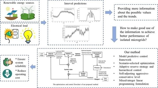
:In this paper, we consider a probabilistic microgrid dispatch problem where the predictions of the load and the Renewable Energy Source (RES) generation are given in the form of intervals. A hybrid method combining scenario-selected optimization and reserve strategy using the Model Predictive Control (MPC) framework is proposed. Specifically, first of all, an appropriate scenario is selected by the optimizer at each optimization stage, and then the optimal scheduling and reservation of system capacity are determined based on the selected scenario and possible variations in the future as provided by the predictors. In addition, a new reserve strategy is introduced to adaptively maintain system reliability and respond to variations in the hierarchical microgrid control. Simulations are conducted to compare our proposed method with the existing robust method and the deterministic dispatch with perfect information. Results show that our proposed method significantly improves the system efficiency while maintaining system reliability.
1. Introduction
Microgrid dispatch receives increasing attention in recent years. On the one hand, proper scheduling of controllable devices in advance can contribute to significant economic benefits while meeting the demand [1,2,3]. On the other hand, the dispatch strategy is vital to maintain adequate frequency stability for microgrids with Distributed Energy Resources (DERs) which introduce undesirable fluctuations [4,5]. When microgrids operate in the isolated mode, adequate frequency performance is much more crucial since the Renewable Energy Sources (RES) such as wind and solar tend to be very volatile [6,7]. Missing the support from the robust main utility grid, it is much more challenging to ensure stability for isolated microgrids.
In microgrid scheduling, there exists uncertainty due to the uncontrollable changes in load consumptions and RES generation. As the penetration level of RES becomes higher, the uncertainty in microgrids also increases, which makes it more challenging to handle, especially for isolated microgrids without the support from the main grid [8]. Therefore, it is very crucial to ensure the operation stability and balance between supply and demand in addition to the consideration of economic performance in microgrid dispatch strategy design.
In the literature, most articles only consider deterministic predictions, where both of the load consumptions and renewable generation are predicted in the form of deterministic values. Then, the dispatch strategy is obtained via the optimization on the single predicted deterministic scenario (see, e.g., [9,10,11,12]). As a result, the performance of the dispatch strategy is highly dependent on the prediction accuracy. Although various efforts have been made to improve the prediction accuracy, the highly volatile nature of the RESs greatly limits what one could achieve in terms of the prediction performance [13,14]. Therefore, the dispatch strategy designed under the predicted scenario would be far from the actual optimal during the operation. Furthermore, system stability could be greatly compromised due to the mismatch between the actual scenario and the predicted one, which would be of great concern for isolated microgrids that are more vulnerable in terms of stability and reliability.
To address the issues caused by the uncertainty in microgrid systems, some probabilistic methods have been proposed recently. For example, Rastegar el. at. applied the 2-point estimate method (2PEM) to model the uncertainty associated with RES generation power, and the household demand was managed by solving the probabilistic optimization problem [15]. In [16], the uncertainty was defined as a Gaussian disturbance and the stochastic control of energy-efficient buildings was considered. In another work [17], non-Gaussian wind power uncertainties were considered by incorporating an upper layer stochastic predictive controller. The uncertainty in the power demand and the RES power output was handled by formulating a two-stage stochastic problem in [18] and [19], where the infeasibility from the first-stage decisions was compensated in the second stage in order to maintain the power balance. In [20], a two-stage stochastic scheduling method was used and the uncertainty of load, wind, and PV generation was captured using Gaussian, Weibull, and Beta distributions, respectively. These works mainly use the stochastic control approach or assume that the uncertainties in the microgrid follow a certain distribution described by probability distribution functions (PDFs). However, high volatility and uncertainty of RES might lead to large errors and increased instability of the system for stochastic control approaches, since they still rely heavily on deterministic forecasting. In addition, the assumptions about the distributions are not always accurate and the complexity for stochastic control could be high for some distributions [21,22]. Hence, these methods are not good candidates for the dispatch in isolated microgrids with high penetration levels of RES and strict stability requirements.
Another type of probabilistic methods has also been reported in the literature. In these methods, instead of a single deterministic scenario, several representative scenarios or intervals are generated to accommodate the uncertainty of the predictions to some extent. For example, for the method in [23], multiple plausible scenarios were generated as the optimization inputs and then the worst-case performance is optimized over these scenarios using the robust Model Predictive Control (MPC) approach. In [24], the authors studied the multi-objective optimal dispatch of microgrid under uncertainties based on the interval optimization approach and Pareto optimality. In [25,26,27], prediction intervals with appropriate width and coverage probability were generated using fuzzy models to represent the uncertainty of future predictions. In [28], Mamdani fuzzy logic systems using -level cuts of the output fuzzy sets were applied to generate uncertainty intervals for each individual forecasting value. In [29], a hybrid method including improved wavelet neural networks and generalized extreme learning machine was proposed for load probabilistic interval forecasting. Another prediction method extended the fuzzy models with neural networks for constructing prediction interval models based on fuzzy numbers [30]. In [31], an affine algorithm was used to model the interval uncertainties, and then new intervals with soft bounds were formed using joint PDFs to reduce conservation and improve feasibility. Using the larger range prediction inputs rather than a trajectory, the obtained dispatch is able to cope with various possible situations and hence improve system reliability. Compared with the deterministic approach, these probabilistic methods better account for uncertainty during the prediction. Compared with the distribution-based methods, they also boast lower complexity.
Notwithstanding the successes of probabilistic methods in handling variability and maintaining stability in isolated microgrid energy management, little work has been done to make good use of the predicted intervals in subsequent optimization to achieve economic benefits. For instance, prediction intervals with different levels of coverage probability were generated in [25,28,29,30], but there were no discussion about how to facilitate them for optimal dispatch. In [26], the authors adopted a robust method towards the predicted intervals and evaluate the performance of generating optimal intervals. However, this strategy was too conservative and resulted in poor economic performance, in some cases even worse than the dispatch without optimization. In [27], the coverage probability could be chosen by designers to adjust the trade-off in terms of constraint satisfaction and energy consumption, but it was not intelligent and flexible. Soft intervals were generated in [31] to handle the confidence level and improve the economic performance, but joint PDFs were used to transform the intervals resulting in a very high computational burden. However, the prediction intervals not only provide the information about the worst cases as these dispatch methods utilize, but also indicate the trends of the situation via the change of the interval widths at different moments. With more sufficient information about the trends, sometimes the system can afford to be more aggressive to reduce the cost, e.g., when the RES generation and load consumptions tend to be more balanced. Therefore, it is worth further investigation on the better utilization of prediction intervals to improve the economic performance of interval-based optimization methods.
To this end, we come up with an approach that utilizes the information provided by the intervals to improve economic performance while maintaining reliability. In this approach, appropriate scenarios are selected according to the prediction intervals to optimize the dispatch so as to reduce the operation cost of the microgrid system. Meanwhile, a reserve strategy is introduced to further utilize the information provided by the prediction intervals to ensure the stability of the system in actual operations [32]. Moreover, MPC is adopted as the framework of the optimization, where the system is optimized over an extended horizon by predicting the system behavior over that horizon [9,33,34]. This leads to improved optimization performance than the traditional way of optimization based only upon the current system operating conditions. The dynamics of microgrid system are taken into account in the longer term and energy management can be conducted in a more economic manner. The hierarchical control strategy is also discussed to further compensate for the differences using reserves. In this paper, the proposed method is also compared with the robust method adopted in [26,35] and the deterministic optimization with perfect information. By the comparison, it turns out that our proposed method is closely related to the existing robust method in the sense that it can be interpreted as a “conditional” robust method, as our optimizer tends to select an extreme scenario conditioned upon the current capability of the system. Simulation results show that our method significantly reduces the operation and reserve cost of the system, while at the same time guarantees capability of the system to deal with various situations. This verifies that our proposed method comprehensively considers both economy and stability.
The major contributions of this paper are as follows:
- 1.
- An MPC-based hybrid method to optimize the probabilistic microgrid energy management with interval predictions is proposed in this work. Compared with the existing methods to handle the interval inputs, our proposed method can further utilize the interval predictions and significantly reduce the system cost while maintaining stability.
- 2.
- A new reserve strategy is proposed to make full use of the resources in microgrids and achieve adaptive security of the system, where the secondary control and the tertiary control in the microgrid system are considered in an integrated manner.
- 3.
- Moreover, reserves are set as decision variables whose values will be determined by the optimization process rather than as pre-calculated constants in most existing solutions. This approach promotes the efficient utilization of resources and further reduces cost.
- 4.
- The discount factor is introduced to the cost function for better performance, and guidance for finding the optimal value of this parameter is provided.
The remainder of this paper is organized as follows. Section 2 presents the models of elements and the control model in a microgrid. Section 3 introduces the reservation strategy proposed to handle the intervals and the formulation of optimization using the MPC method. Simulations on a typical isolated microgrid system are conducted and the results are discussed in Section 4. Finally, the conclusions of this paper are summarized in Section 5.
2. System Model
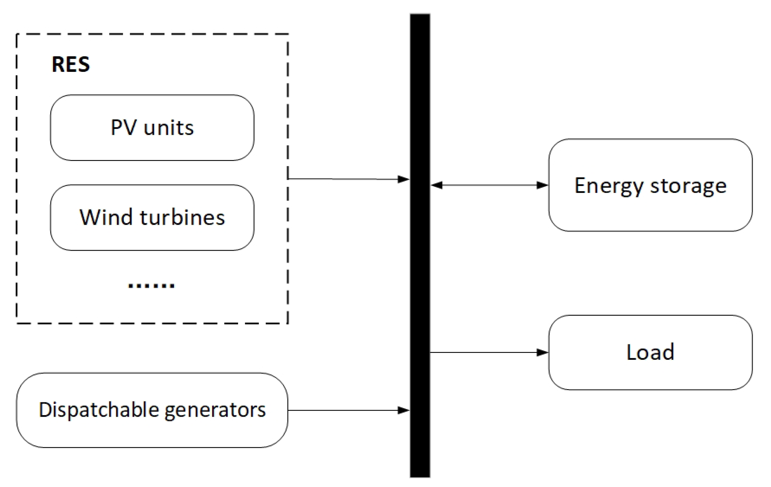
A typical microgrid system is usually composed of several types of elements including loads, dispatchable generators, non-dispatchable RESs such as photovoltaic (PV) and wind turbines (WT) and energy storage as shown in Figure 1. For optimal dispatch, one needs to first predict the power of RES generation and load consumption, and then optimize the operation of the storage units and generators to achieve the maximum economic benefit while maintaining the system stability. In the following, we introduce the model for each type of these elements and the control model in the microgrid.
2.1. Renewable Energy Sources
RES is a key element in microgrid operation. On the one hand, one wants to make the best use of RES resources because they are renewable, environmentally friendly, inexhaustible, and economical. On the other hand, however, they are uncontrollable, non-dispatchable, and intermittent with high variations. These bring a lot of challenges to their grid integration. To utilize the resources more reasonably, we need to forecast their generation and take this into account during the dispatch optimization.
Some researchers predict the local sequential data of solar and wind speed and then calculate the generation power according to some energy transfer equations [10,36], while most papers study the history of RES generation and directly predict the generation power. Regardless of the data sources and the underlying principle for forecasting, many studies use stochastic or probabilistic prediction methods in order to better account for the variability of RES. Among those, we pay special attention to the interval predictions. For example, in [25,26], fuzzy interval models were used to generate appropriate prediction intervals of photovoltaic power generation and wind power generation with optimal width or coverage probability. The interval predictions for one-step ahead to one-day ahead the paper [25] generates for microgrid dispatch have 90% of confidence level with about 3.67% maximum relative error in photovoltaic power generation and 8.85% maximum relative error in wind power generation. In general, for those interval predictors, the power for RES generation could be described as:
where k is the discrete-time index, and are the generation power of photovoltaic generators and wind turbines; the underline and the overline of power variables denote the lower and upper boundaries of the prediction intervals, respectively. Without loss of generality, only solar and wind are listed here. Other forms of RESs could be defined similarly.
2.2. Loads
The prediction interval of loads can be obtained similarly as introduced in Section 2.1 by some probabilistic forecasting methods. For instance, the load intervals with 90% confidence level predicted for one-step ahead to one-day ahead in the paper [25] have about 3.67% maximum relative error. In general, the predicted power for loads could be represented as:
where is the predicted power of loads; the underline and the overline of denote the lower and upper boundaries of the load prediction interval, respectively.
2.3. Storage Units
Following the practice in [10], we use the following discrete-time model to describe the storage dynamics:
where is the energy stored at time k; and are charing and discharging power; denotes the loss rate with respect to stored energy degradation in each sampling interval and is the efficiency of charging/discharging with .
Here, we introduce two reserve variables and to represent upward reserve power for charging and downward reserve power for discharging, and two binary variables, and to indicate the charging or discharging states of batteries with constraint
Using the big-M method [37] to avoid the bilinear problem, the power flow limits can be written as
2.4. Dispatchable Generators
Dispatchable generators are sources that can be used flexibly on demand, including diesel generators, natural gas turbines, oil-fed generators, and so on. These generators can operate almost anywhere at any time so long as relevant constraints are met. However, their operating costs are usually high and there are strict limits on their ramp up and ramp down rates. As a result, the usage of dispatchable generators should be carefully planned to reduce cost, avoid violations and coordinate supply with demand when necessary.
Binary variables are introduced to describe the ON/OFF state of dispatchable generators:
with where is the number of generators. Then, the operating constraint can be expressed as
where is the operating power of ith generator, and and denote the minimum and maximum power level, respectively.
After introducing the reserve variable denoting the upward reserve power of the ith generator for generating and using the big-M method, constraint (7) can be transformed into the following linear inequalities:
We also model the startup and shutdown behavior of the generators in order to calculate the corresponding cost. To this end, two auxiliary variables and are introduced, denoting the startup cost and the shutdown cost of the ith generator at time k. The following constraints must be satisfied:
where and are coefficients of startup and shutdown costs of the ith generator, and denotes the maximum ramp up and ramp down rates.
2.5. Hierarchical Control
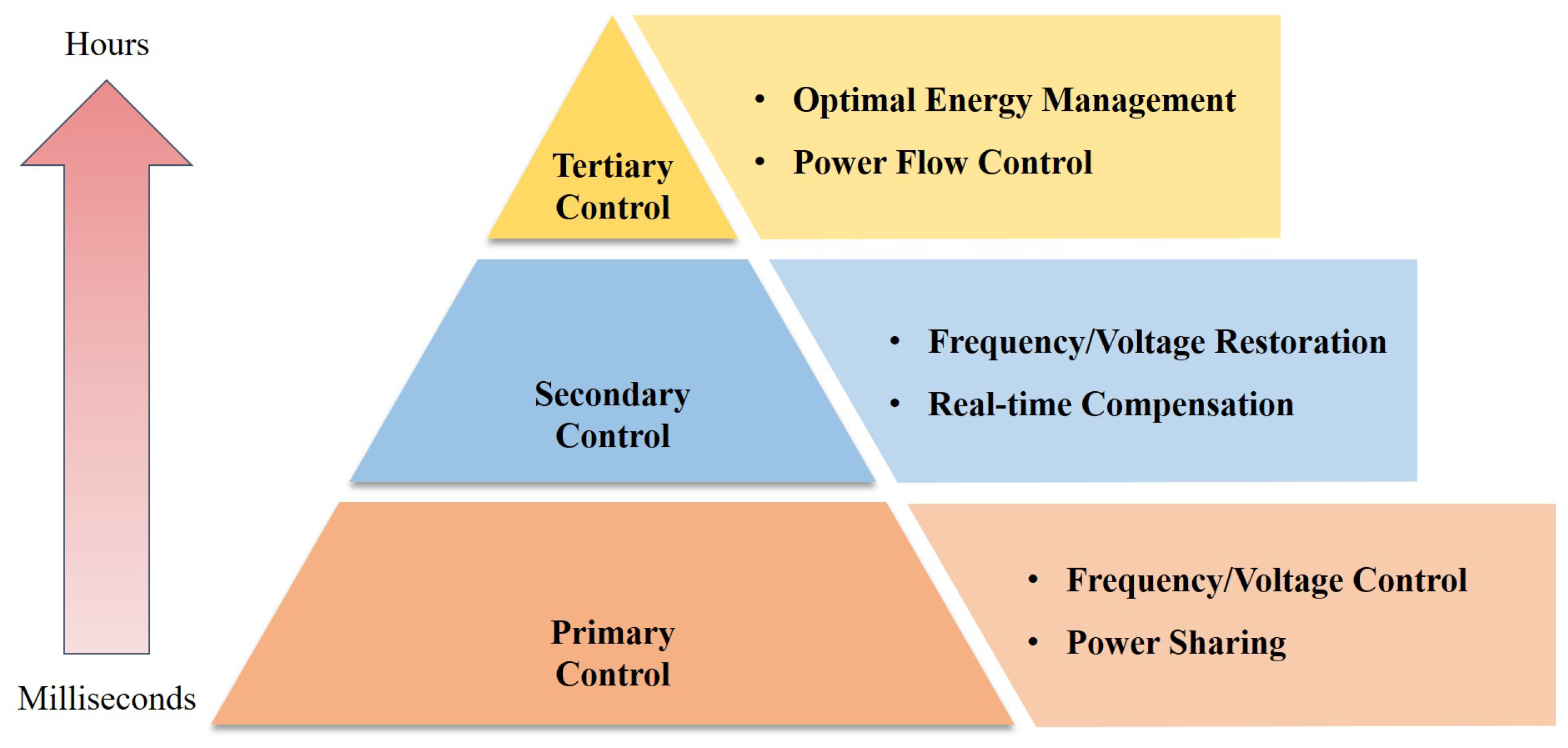
The hierarchical control model is widely applied for the operation of isolated microgrids [38,39]. Traditional hierarchical microgrid control is generally divided into three levels, including primary control, secondary control, and tertiary control as shown in Figure 2 [40]. These three control levels are relatively independent and responsible for their respective functions, but in the meantime, interconnect and coordinate to accomplish the integrated control of the system [41,42].
The primary control, which belongs to the local control category, focuses on stability maintenance and autonomous operation. Droop control is typically used at this level in isolated microgrids to adjust the frequency and voltage and ensure that the actual value tracks the reference value.
However, in the islanded mode, the voltage and frequency of the microgrids vary with the load, and the primary control is usually insufficient to maintain the system frequency. As a result, the secondary control is required to compensate for the fluctuations in frequency and voltage. The secondary control can monitor the frequency and voltage amplitude of the microgrid and detect the load, based on which it adjusts the load reference value and compensates the power to restore the system frequency.
The tertiary control is the control at the top layer. It is mainly for the energy management system of microgrids, which accomplishes the economic operation of microgrids with the use of various optimization methods. The tertiary control is the control strategy with the largest time scale, generally on the order of 5 min to 2 h.
This paper focuses more on the optimal dispatch problem at the tertiary control level, but, at the same time, an improved secondary control is needed to further respond to loads and compensate for variations. The primary control is also important in the system, but we devote no particular discussions on it and assume that it can successfully provide the basic functions here. Note that the time-scale of the secondary control is in the order of 1 to 10 s, which is far less than the time-scale of the tertiary control, hence specific formulas will not be shown and used in the optimization. Instead, we can regard it as an almost instantaneous action when solving the economic dispatch problem and only need to specify the corresponding regulation strategy for it, which will be discussed in the next section in detail.
3. Optimal Dispatch Problem
In this section, the MPC-based optimization with reserves for the isolated microgrid optimal dispatch is discussed. The new reserve strategy and the related hierarchical control strategy are also presented.
3.1. Model Predictive Control
MPC is a receding horizon method used to control a process while satisfying a set of constraints [33,43]. At each step, a constrained optimization problem over an extended horizon is solved to produce the system schedule. Then, the first action in the schedule sequence is executed and information is updated after feedback. At the next step, another optimization problem is solved over the receding horizon using updated inputs and the same process is repeated until the end of the process.
For the discussed interval optimization problem with reserve strategy, we perform the following steps to apply the MPC method to minimize the operation costs:
- (1)
- Predict. At time step k, predict the power intervals of PV and WT generation and load demand over time horizon .
- (2)
- Optimize. Solve the constrained optimization problem using the predicted intervals as inputs and obtain the optimal dispatch sequence from step to step .
- (3)
- Execute. Operate the system based on the first action in the optimal dispatch sequence, and adjust the controllable devices according to the actual error to compensate the error.
- (4)
- Roll ahead. Update the system information. Then, roll the horizon ahead and repeat the steps above over time horizon .
Repeat until the process is finished.
3.2. Reserve Strategy
The rationale of the reserve strategy in this paper is to reserve certain capacity of the devices in advance to ensure that the system has sufficient capacity even if the actual situation is far different from the predicted. This improves the stability and reliability of the system.
In order to ensure the safe and reliable operation of microgrids, sufficient reserve power should be available. In this way, the microgrids can use reserves to restore system frequency under the secondary control when the system power is unbalanced. In general, the size of the reserve power is fixed, which can be calculated before the optimization in the tertiary control level depending on the size of imbalance and the schedule changes [39]. However, it is unreasonable to set the reserves as constants in practical system operation due to the variations of loads and RES generation. In order to make full utilization of the resources in the isolated microgrids and reduce the system cost, we change the reserves of controllable devices to variables. Moreover, they are introduced into the optimization as decision variables so that their values can be determined by an optimization process under different scenarios to ensure system stability in time.
In the models of storage units and dispatchable generators, three reserves , , and are introduced as extra control variables, denoting upward reserve power for charging, downward reserve power for discharging, and upward reserve power for generating, respectively. These reserve variables should satisfy the following constraints:
with
where and represent the maximum power error between the actual value and the selected predicted value in optimization in the conditional best case and worse case, respectively.
Note that there is a trade-off between the reserves and the scenarios selected by the optimizer. The optimizer tries to reduce the operating cost as much as possible while the corresponding reserves hinder the possibility of further cost reductions in order to ensure certain capability of the system to maintain adequate frequency stability. Therefore, we can find the best balance in the optimization by adding a penalty to the level of reservation.
3.3. Optimization Formulation Based on MPC
The objective of the optimization is to minimize the total cost of the microgrid system. The cost function contains operation and maintenance costs, energy production cost, startup and shutdown cost, and reserve cost:
where t denotes the current time, and k is the step index; M is the length of time horizon; is the discount factor we introduce with . The discount factor is mainly used for infinite horizon problems, in general, to determine the horizon [44,45]. Here, we use it to adjust the weight of steps. Dispatch in the near future is given higher priority and steps in the distant future would affect the system decision less. The reason for this is that interval predictions only provide an approximate range of possible values that RES generation and load may take, and the prediction error would be accumulated over time. For example, the prediction after dozens of hours would be very inaccurate and have great potential to change as the horizon rolls on. Therefore, we reduce the weight of the latter steps and focus more on the near future in the optimization.
In the formulation, the operation and maintenance cost is
and the energy production cost of dispatchable generators is
the startup and shutdown cost is
and the reserve cost is
Here, is the time duration of each step; and are corresponding coefficients for battery, and , and are corresponding coefficients for dispatchable generators; and are coefficients for penalties.
In addition, the system needs to satisfy the condition of power balance:
Finally, the problem in the MPC framework is formulated as a mixed integer linear programming (MILP) optimization problem. It is known that MILP is NP-hard rather than NP-complete when it is considered as an optimization problem [46,47], and the required computational efforts mainly depend on the number of integer variables [48]. Branch-and-cut combining cutting planes and branch-and-bound methods are one of the efficient approaches for solving MILP problems [49,50]. Presolve, Lagrangian relaxation, and heuristics are also introduced to tighten formulation, transform the combinatorial problem and find better initial solutions so that the problem size and the computational complexity can be significantly reduced [51,52]. There is an advanced solver integrating these methods provided by Gurobi, which can solve the general MILP problems fast [53]. In this paper, we will facilitate the existing solver for our problem.
3.4. Hierarchical Control Strategy
There are three levels in the hierarchical control, which are primary control level, secondary control level, and tertiary control level. They perform their respective duties and coordinate to achieve economic and reliable operation.
First, the optimal scheduling sequences based on the selected scenarios are obtained in the optimization stage at the tertiary control level, which are sent to the primary and secondary levels for execution. Elements in the microgrid will operate according to the optimal reference values, but due to the inevitable differences between the predicted and the actual values, it is impossible to meet the power balance by only executing in full accordance with the scheduling scheme in practice. Therefore, the secondary control is required to respond to the variations of load and RES power generation, so as to compensate for the errors and ensure the system frequency stability. It is noted that the actual compensation power is limited by the decision values of the reserve variables, which can be presented as
where is the actual compensation power of the battery and may take a positive or negative value within the limit; is the actual compensation power of ith dispatchable generator (DG) and can only be nonnegative, which means it is used only when additional power generation is needed.
| Algorithm 1 The control strategy in secondary level. This strategy instructs the compensation operation for the further variations using reserve in secondary level of the hierarchical control. |
| Input: The operating power of ith generator ; the charging and discharging power of battery |
| units and ; three reserve variables , and ; |
| Result: |
| 1: Set the power reference value for controllable devices, i.e., , ; |
| 2: Detect the differences between the actual situations and the selected scenarios; |
| 3: Obtain the total power that need to be compensated ; |
| 4: if then |
| 5: until |
| 6: else |
| 7: until |
| 8: if then |
| 9: until |
| 10: end if |
| 11: end if |
| 12: The acutal operating power of battery |
| 13: The acutal generating power of ith DG |
| 14: The violation power |
| 15: return |
| 16: Next, step |
In order to compensate for the differences between actual situations and selected scenarios in an orderly manner and increase the economic benefits, we also set a simple but effective strategy for the secondary control, the major part of which is shown in Algorithm 1. Firstly, the power value that needs to be compensated to the system is calculated according to the actual state of the system. If the value of the compensation power is negative, which means the actual total power generation is higher than the load demand, the redundant power will be stored in the battery using the part of the upward reserve power for charging; if the value of the compensation power is positive, which indicates that the actual power generation cannot meet the load demand, more power should be generated. In the operation of increasing power generation, there is a priority list of the battery units and DGs with different rated power. Reducing the charging power or increasing the discharging power of the battery is the highest priority overall because the associated cost is less. However, when the reserve power of the battery is fully consumed, the demand needs to be compensated by adjusting the generation power of DGs. The regulation at this point follows several rules: (1) use the reserves of the running DGs first (as there exists the startup cost); (2) if more than one DG is running, the reserve power of DG that has the highest rated power is preferred; (3) if more than one DG has been turned off, but it is needed to start one DG to increase power generation, DG that has the lowest rated power is preferred (because DG with higher rated power has higher startup and shutdown cost). These three rules are easy to understand intuitively, but to make the process concise, the detailed control is not shown in Algorithm 1, Line 13.
4. Simulation Results
To verify the performance of our proposed method, co-simulations are conducted using MATLAB 2017b, YALMIP (Version 25 April 2019) [54] and Gurobi 8.1 [55]. The system model is implemented using Matlab. The optimization problem is modeled using YALMIP and solved using Gurobi based on the Branch-and-Bound methods [46,56]. The program was executed on a Super Server 4028GR-TR2 with 2 Intel(R) Xeon(R) E5-2698v4 processors at 2.20 GHz and 16 GB of RAM memory in Shenzhen, China. The scheduling results and the optimization strategy of our proposed method are discussed in this section. Its economic performance is also evaluated compared with the existing robust method. The parameters used in the simulations are summarized in Table 1.
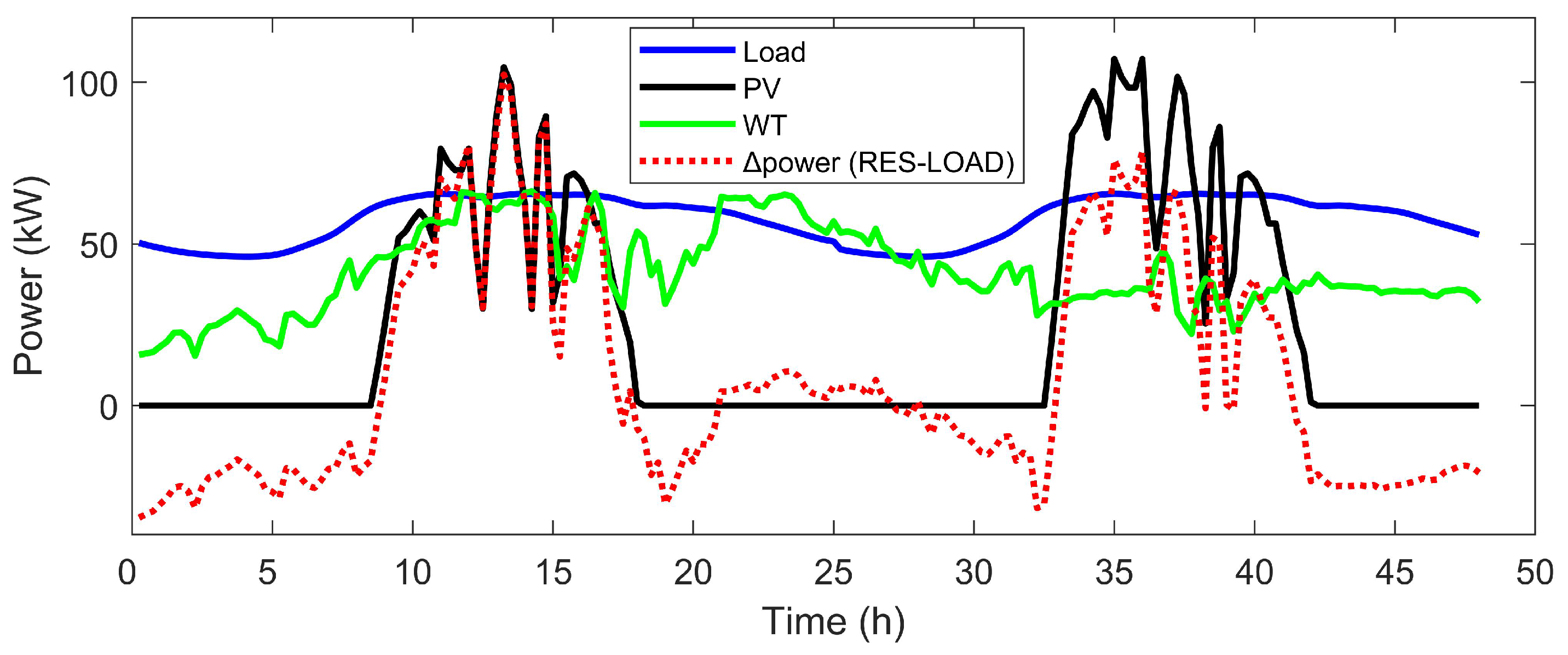
The microgrid we consider in the simulations is working in the isolated mode, consisting of a photovoltaic system, a wind turbine, a storage unit, and three diesel generators. The study is over a 24-h period with 15-min intervals as Table 1 shows, but the MPC framework we applied requires the data for the next 24 h after the current time, so we actually use two days of data. We choose two typical days for simulation, and the actual data of load, PV, and wind turbine power for 48 h are shown in Figure 3. power is the difference between RES generation and load demand showing the power that needs to be compensated by the generators or storage units. It can be seen that this set of data contains almost all the typical cases with proper fluctuations. In addition, the storage device is bounded between 10 and 200 kWh with maximum charging and discharging power 150 kW. The charging and discharging efficiency parameter is 0.9, and the loss rate with respect to stored energy degradation in each sampling interval is 0.05. The three DG units have different rated powers 20, 40, and 60 kW respectively, and their ramp up and ramp down rates are 8 kW. The shut up and shut down costs of them are 5, 10, and 15 each time, respectively. In addition, the value of the discount factor is 0.8.
The system parameters are selected based on several system performance indicators such as loss of power supply probability, levelized cost of energy, and level of autonomy [57], and also referring to the setting of case studies in some papers [9,10]. The penetration level of RES is also considered, which is more than 90 percent with our system setup. As for the four simulation parameters, the discrete time step and the rolling horizon are set on the basis of the literature of typical microgrid optimal dispatch problems using the MPC method [9,58]. The time step is set to 15 min mainly due to the common considerations of optimization and available predictions for the load demand and RES generation. Long horizon may increase the computational complexity and reduce economic efficiency, but it should be sufficiently long to provide a stable controller and ensure the feasibility [59]. The duration of simulations is set to 24 h since we aim at improving the economic performance of the microgrid over a long time period, where day-ahead problems are mostly concerned. Therefore, the total operation steps in one day is 96 given the time step.
In Section 4.1, we demonstrate simulation results using our proposed method mentioned above to optimize the probabilistic microgrid dispatch problem with interval predictions. In Section 4.2, simulations using the existing robust method are shown for comparison. Section 4.3 compares the economic performances of the proposed method, the robust method, and the deterministic MPC-based optimization method. Section 4.4 studies the effect of the discount factor and Section 4.5 analyzes the strategy of scenario selection and the reserve strategy in the optimization stage of our proposed method. In Section 4.6, we conduct a sensitivity analysis to verify the reliability of our proposed method.
4.1. Case 1: Probabilistic Microgrid Dispatch Using Our Proposed Method
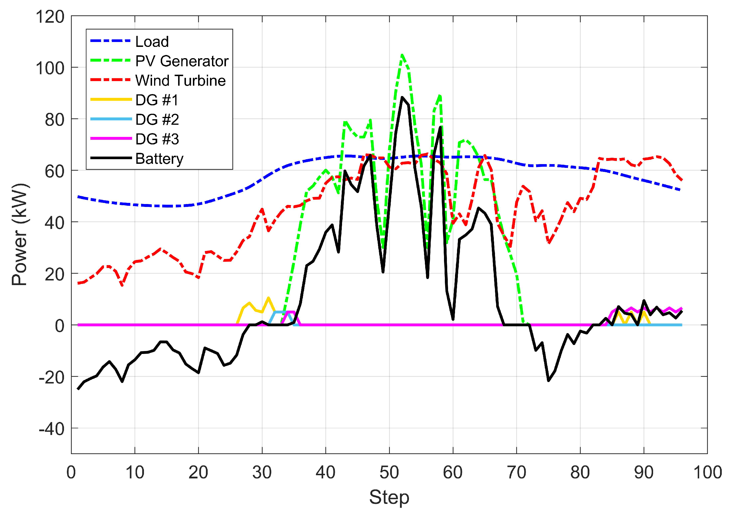
The simulation results of one day using our proposed method are shown in Figure 4. The dashed curves of load, PV generator, and wind turbine describe the actual data in 24 h in Figure 3. By comparing the four solid curves which are the DG and battery dispatch results, we can see that the system tends to maximize the usage of battery to save the operation cost. In addition, when the RES generates an insufficient amount of power for a long time, e.g., around steps 30 and 90, the DG units begin to work to meet demand. The shut up and shut down costs of the three DG units are increasing, and we can find that the system tends to use the smaller generator first because of economic considerations.
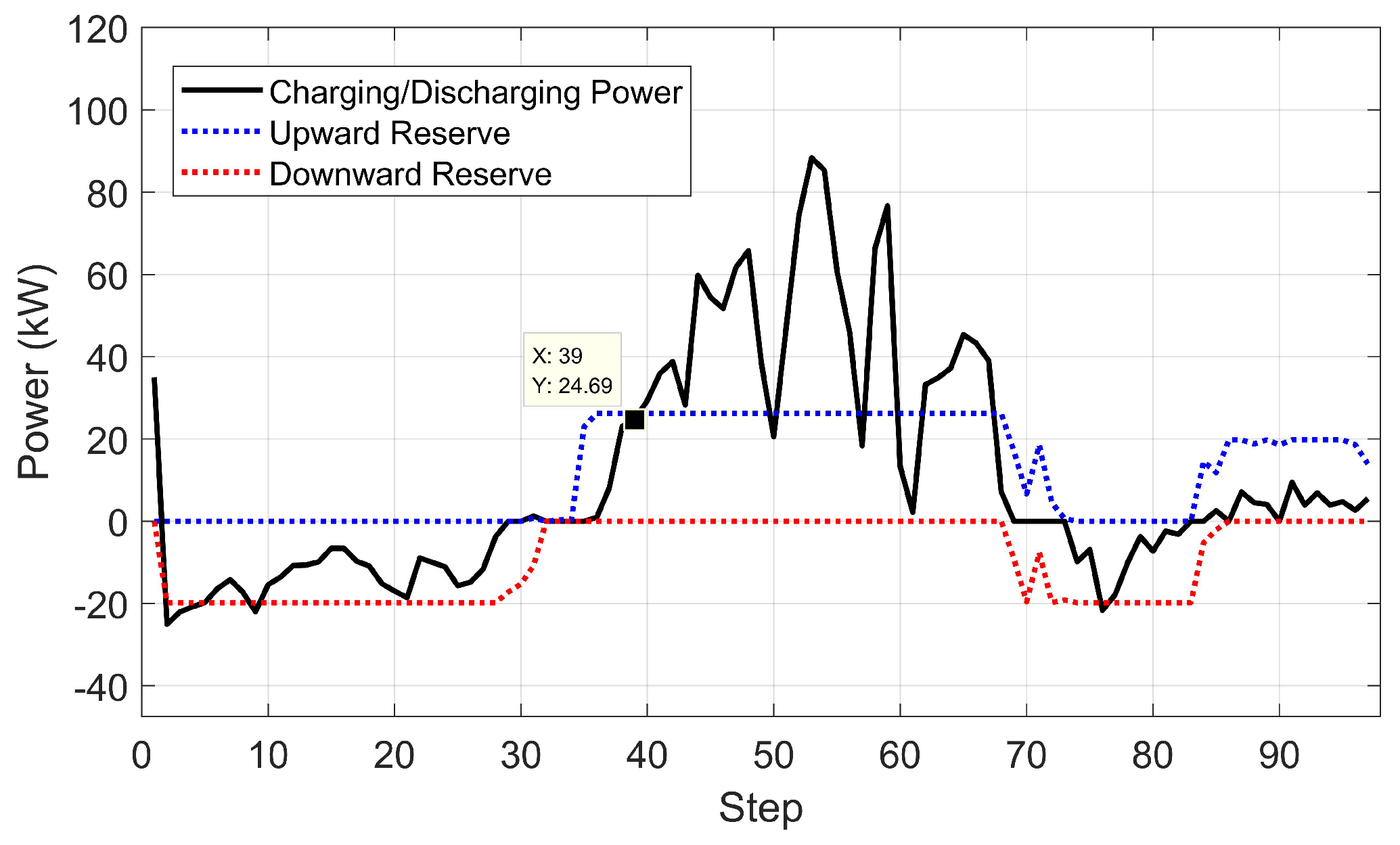
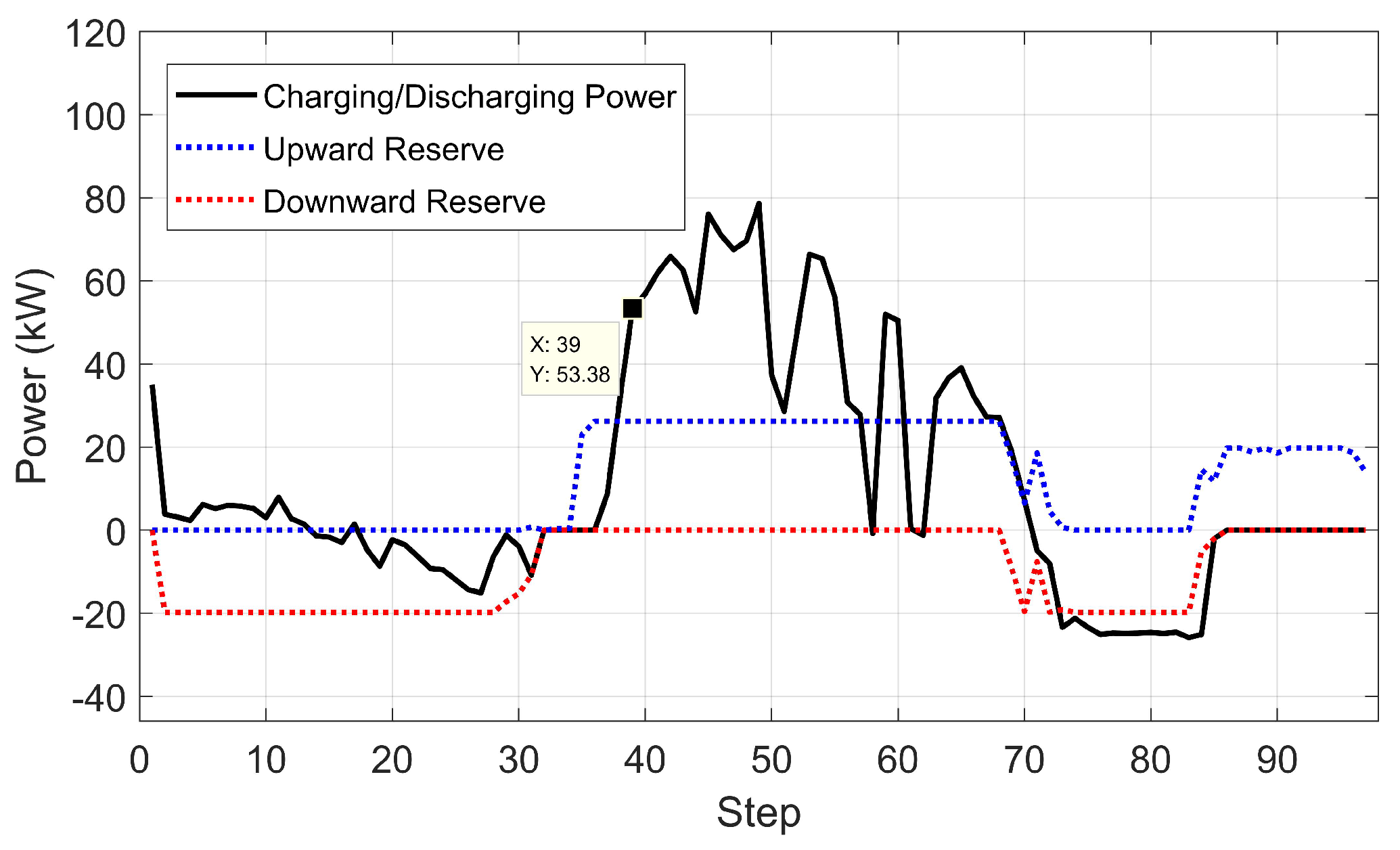
Figure 5 and Figure 6 show the dispatch and operation results of the battery using our method, where the former are the results of optimization step by step based on the scenarios selected by the optimizer, and the latter are the actual operation in practice in the presence of compensation for error using the reservation. It can be seen that the curve in operation changes more sharply than that in dispatch from step 37 to step 50. According to the actual data and the dispatch results, the actual situation is worse than the scenarios we select in optimization during this period, but the system still has the ability to handle the error, which proves the reliability of our system in response to variations. It also illustrates the effectiveness of our method which applies reserve strategy to reserve certain capacity of the system to handle possible variations based on the scenario selected in optimization.
4.2. Case 2: Probabilistic Microgrid Dispatch Using the Robust Method in the Literature
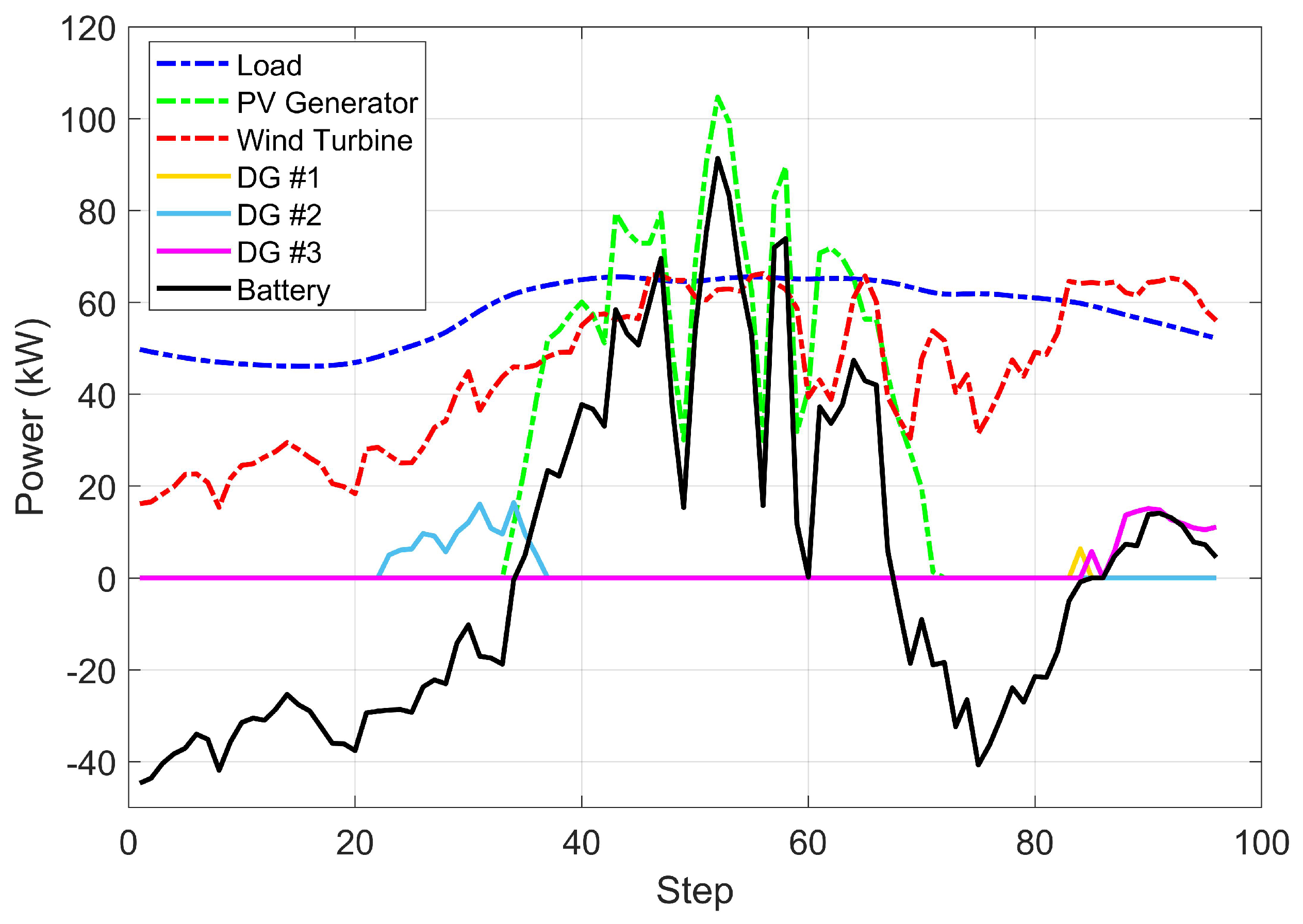
Figure 7 shows the simulation results using the robust method in [26] for probabilistic microgrid energy management with interval predictions. It can be easily seen that the charging and discharging power of battery change more dramatically with a larger variation range compared with the results of our method. In particular, the range of discharging power doubled over the duration. In addition, the system tends to use the largest DG unit more since it always considers the worst case and has to use the largest DG unit to meet demand. This kind of behavior leads to unnecessary increases in costs. The robust method performs not so well when it comes to the economy, although it can ensure adequate frequency performance of the system.
4.3. Performance Comparison
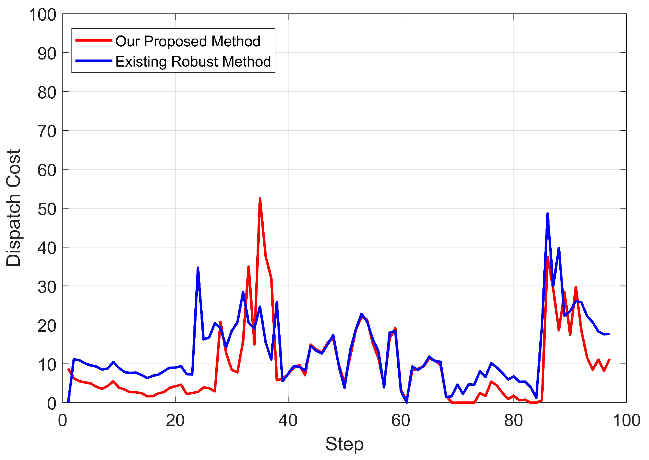
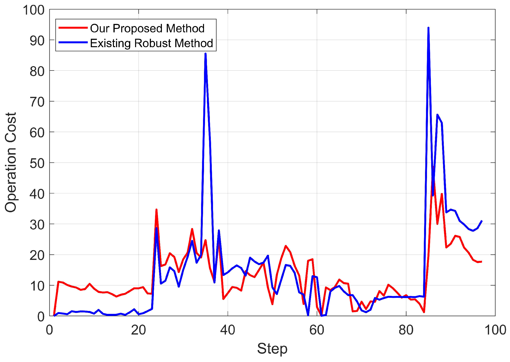
The dispatch and operation costs of our proposed method and the existing robust method are shown in Figure 8 and Figure 9. It is observed that the costs of our proposed method are less than those of the robust method for most of the time. Moreover, the actual operation cost is higher than the dispatch cost for both methods as we expect.
Recall that the first three terms in the cost function (13) are operation and maintenance cost, energy production cost, and startup and shutdown cost, which are the actual operation costs related to the status and working power of devices. In contrast, the last term in the cost function, the reserve cost, is a virtual cost only designed to guide the optimization process. Hence, the operating cost of the system is the summation of the first three terms in the total duration regardless of the penalty term and the discount factor, which is
where the three costs included in the summation are computed using Equations (14)–(16) with the corresponding power at the current time t.
Both the dispatch and operation costs are calculated using Equation (20), but the power used may be different. The dispatch cost depends on the optimal scheduling scheme, and only the first action of the scheme at every current time t contributes to it. However, we don’t schedule dispatches for all the scenarios covered by the interval predictions. Instead, we only select one appropriate scenario and conduct optimization based on it, and meanwhile prepare corresponding self-adaptive reserves to compensate for the difference. In other words, the energy management system will adjust the status or operation power of each device according to the hierarchical control strategy formulated in advance at the operation stage. This leads to a different operating situation in practice, and as a result the actual power and the cost in operation are different from those in dispatch. Moreover, the operation cost is larger than the dispatch cost most of the time, as our proposed method tends to be optimistic to some degree in the appropriate circumstances by putting some load pressure on the prepared reserves so that it can further reduce the cost.
The total costs for one day using different methods are shown in Table 2. The simulation of the deterministic MPC-based optimization method with perfect information of the load consumption and RES generations is also added to serve as a benchmark. It should be noted that there is a certain level of randomness in the prediction and simulation results vary for different trails. Therefore, here, we repeat simulations of each method dozens of times and calculate the average costs for comparison. The optimal scheduling problem has been approximated to a MILP problem, and it doesn’t consume much computational efforts to implement the simulations, where each simulation only takes about 30 min for the presented one-day test, taking less than 20 s to obtain the optimal day-ahead scheduling sequence in the 15-min time step. From the results, we can see that our proposed method has a 23.9% reduction in dispatch cost and an 8.0% reduction in operation cost compared with the robust method, while maintaining the same system reliability. As for the deterministic baseline, our method also reduces 21.1% dispatch cost and 7.0% operation cost. In short, our proposed method achieves the best performance in terms of economic performance.
4.4. Effect of the Discount Factor
The discount factor is worth further discussions. It is observed that the value of this parameter could influence the performance of our method. At the very start when decreases from 1, our proposed method begins to consider more about the current situations and the cost performance becomes better. While as we continue to decrease , the trend goes into reverse. It implies that there might be an optimal value of , where our proposed method could handle the level of preference exactly to minimize the impact of cumulative error while considering the future in advance.
More interestingly, when we introduce the discount factor into the cost function of the robust method and the deterministic MPC-based optimization with perfect information, we obtain similar results. Details can be seen in Table 3 and Figure 10.
We can see that our method performs excellently around , and the operation cost of the MPC-based optimization method also decreases slightly as goes from 1 to 0.8. When is larger than 0.8, the cost of the perfect information dispatch increases rapidly, and even the smallest cost of our method is larger than the average cost when . This illustrates that, when is large, the system focuses more on the future, making it difficult to achieve lower cost in the operation at present, and when is smaller, the system cares more about the current steps so that it can reduce the operating cost by preparing less for the uncertain future. This property also leads to the violations when is too small (less than 0.7 in our simulations), as the system prepares less in advance and may not able to cope with huge variations especially when the actual situation deviates significantly from the expectations.
It can also be inferred that, with the given data and simulation setup, our method could achieve the optimal performance when is somewhere around 0.8, and the conclusion is consistent with that of the dispatch with perfect information. It should be noticed that there is no randomness in the optimization with perfect information since the prediction inputs are just the exact actual data. Therefore, the performance curve of the dispatch with perfect information could give some guidance to find the optimal value of parameter , which could be obtained by simply simulating with different only once.
4.5. Strategy Analysis for Scenario Selection and Reserve
After the comparison, we further analyze the behavior of the scenario selection and reservation allocation strategies of the optimizer in our proposed method.
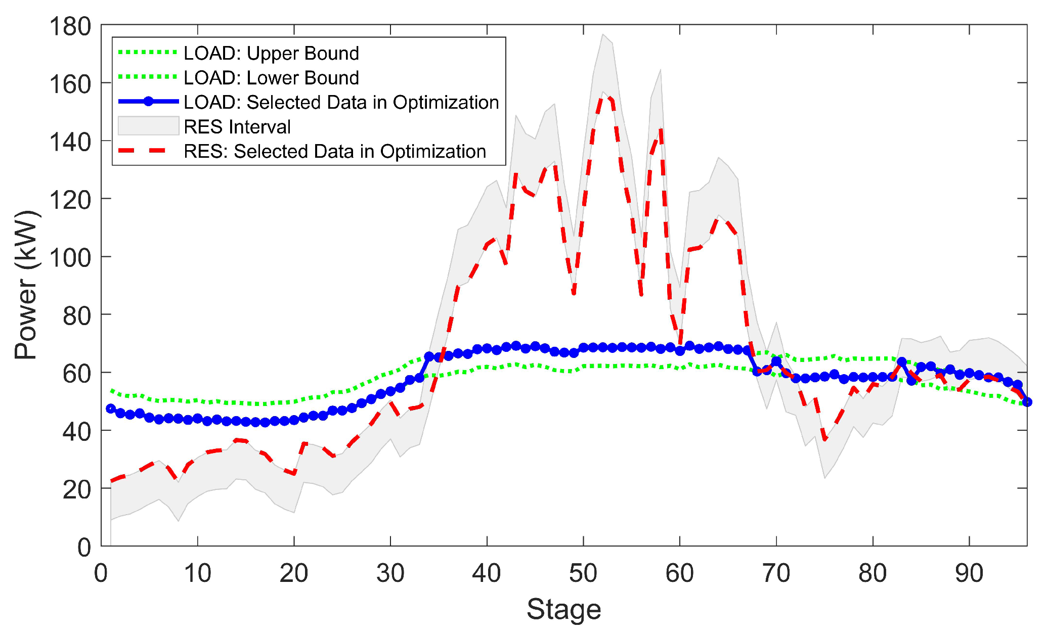
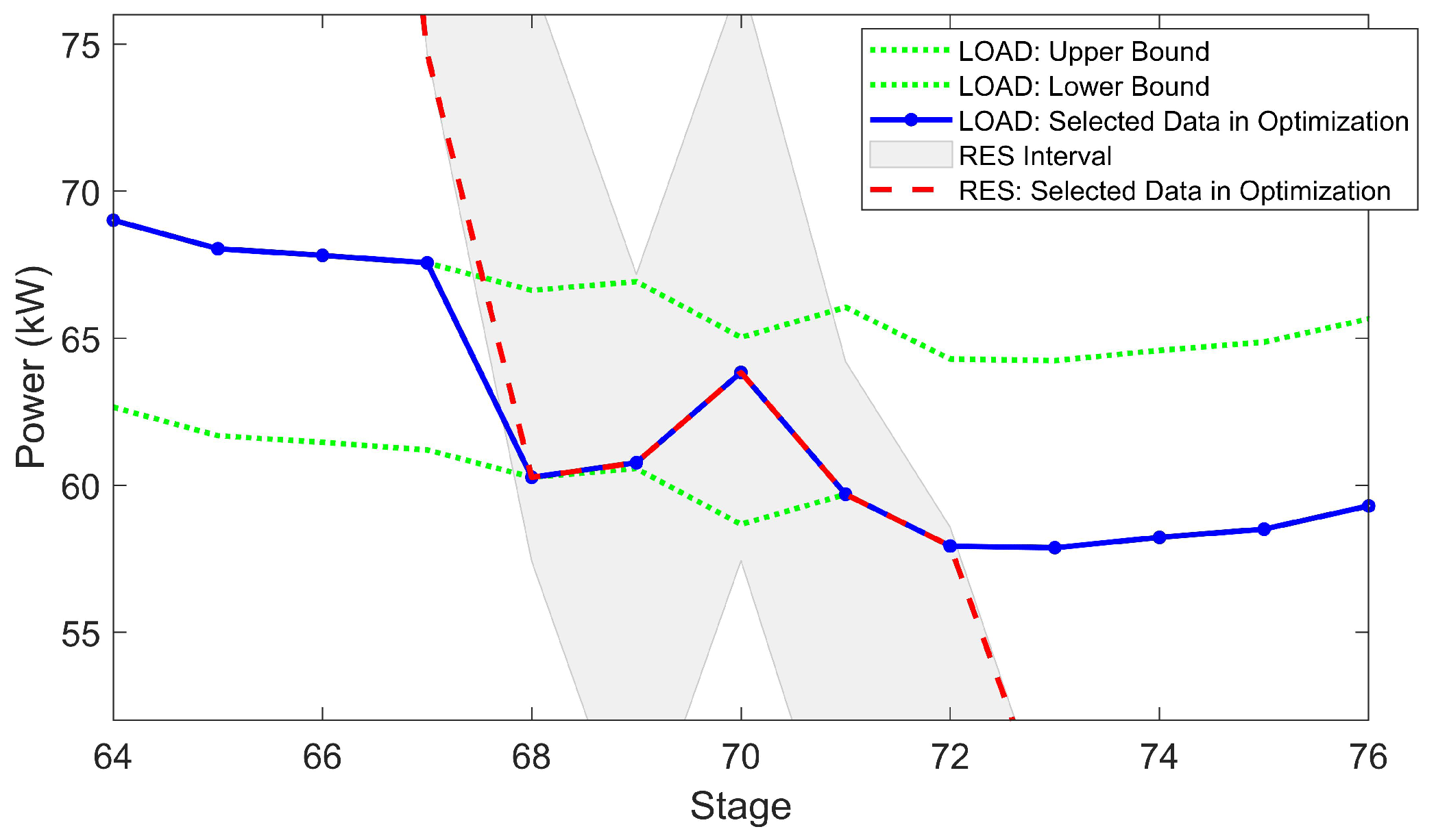
In Figure 11, we integrate the PV and WT generation power and only observe the prediction intervals together with selected values of RESs and load. It can be seen that the system tries to meet the balance between RES generations and load demand so that the cost of extra operation is reduced. When RES generation is high, the optimizer tends to consider the robust situation of load; when RES generation is low, the optimizer is no longer greedy, and it begins to select an appropriate situation of load as the basis for optimization according to the system capacity. This behavior can be seen more clearly in Figure 12 where the area from step 65 to step 75 is zoomed in. It turns out that our method could be explained as a conditional robust method in terms of the behavior of the optimizer, as the optimizer tends to select an extreme scenario based on the capacity of the system. In other words, when the system is in good capability to handle future uncertainty, our proposed method makes the system to prepare for the worst condition; when the system is incapable of handling too much uncertainty, our proposed method allows the system to prepare for a relatively better condition to reduce the cost. It should be noticed that, even though the system is not always preparing for the worst condition, the system stability can still be maintained well due to the fact that there are still energy storage devices and dispatchable generations. This validates the advantages of our proposed method.
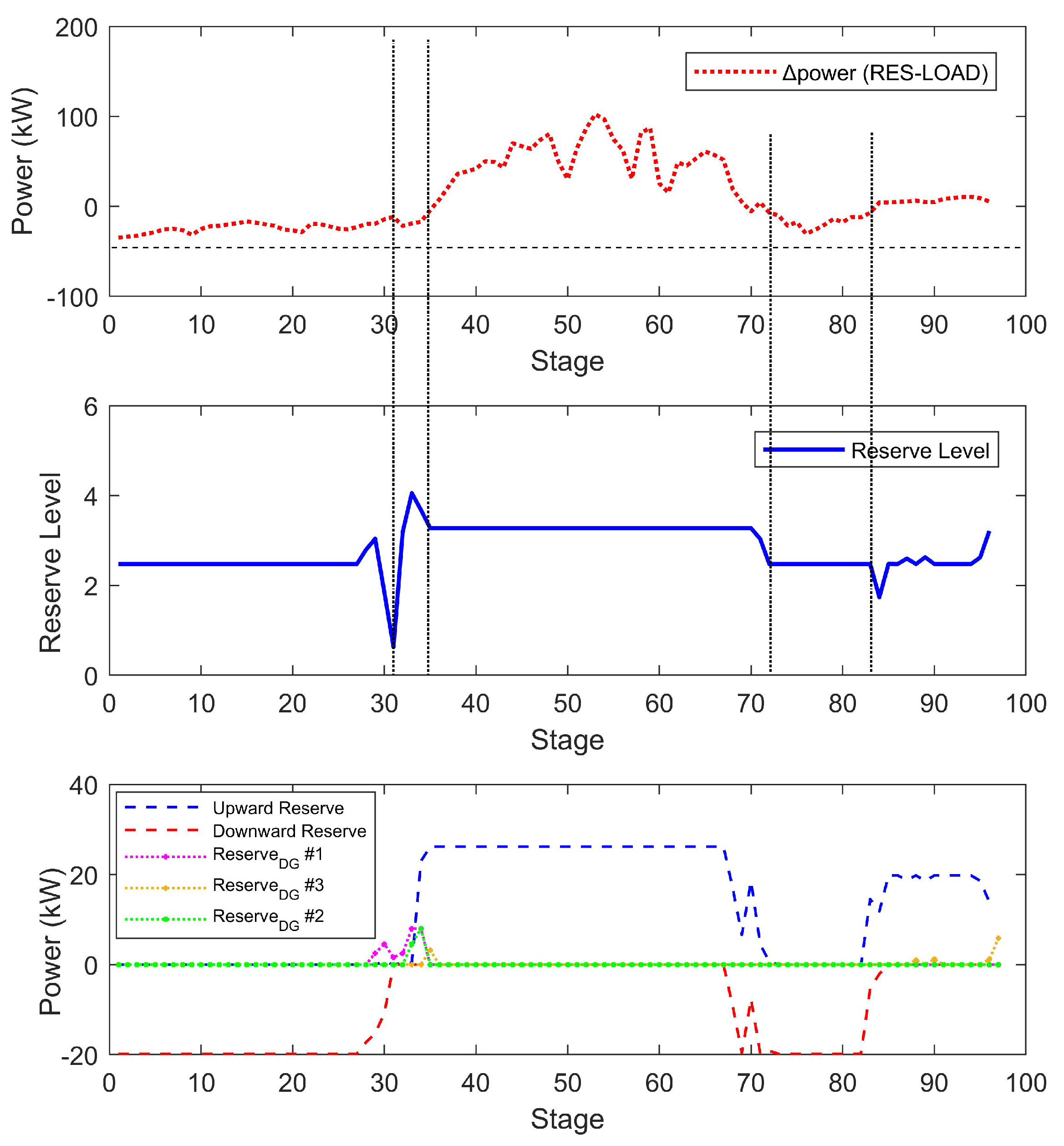
We also analyze the behavior of our reserve strategy. It should be noted that the values of reserve variables are not entirely dependent on the differences between the scenario selected by the optimizer and the worst scenario. According to Section 3, there is also a trade-off between reserves and selected scenarios. In other words, the optimizer tries to find a good trade-off between reliability and efficiency of the system. As we can see in Figure 13, the level of reserve varies with situations. It is not flat and does not always change with the fluctuations. It decreases when RES generation can meet the demand, and increases when the difference between RES and load is large. This shows another effort that our method makes to save costs in some ways.
4.6. Sensitivity Analysis
To verify the reliability of our proposed method, a sensitivity analysis is also conducted to observe the variations of results in different situations. Note that the only uncontrollable factors that would impact the scheduling results of our method are the load demand and the generation of RES. Therefore, we change the actual power data of load, PV generation, and WT generation, and then feed them into the system model as the new actual data and finish the one-day optimal dispatch and control using our proposed method.
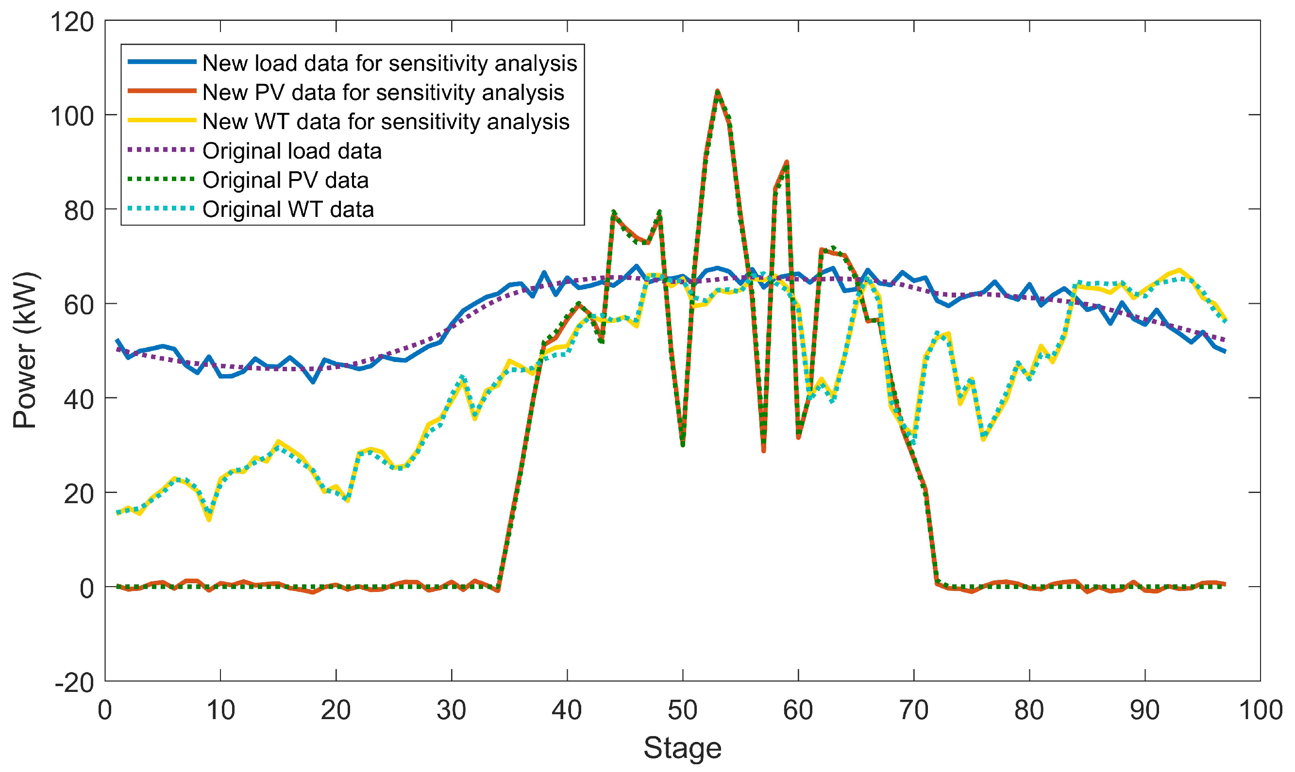
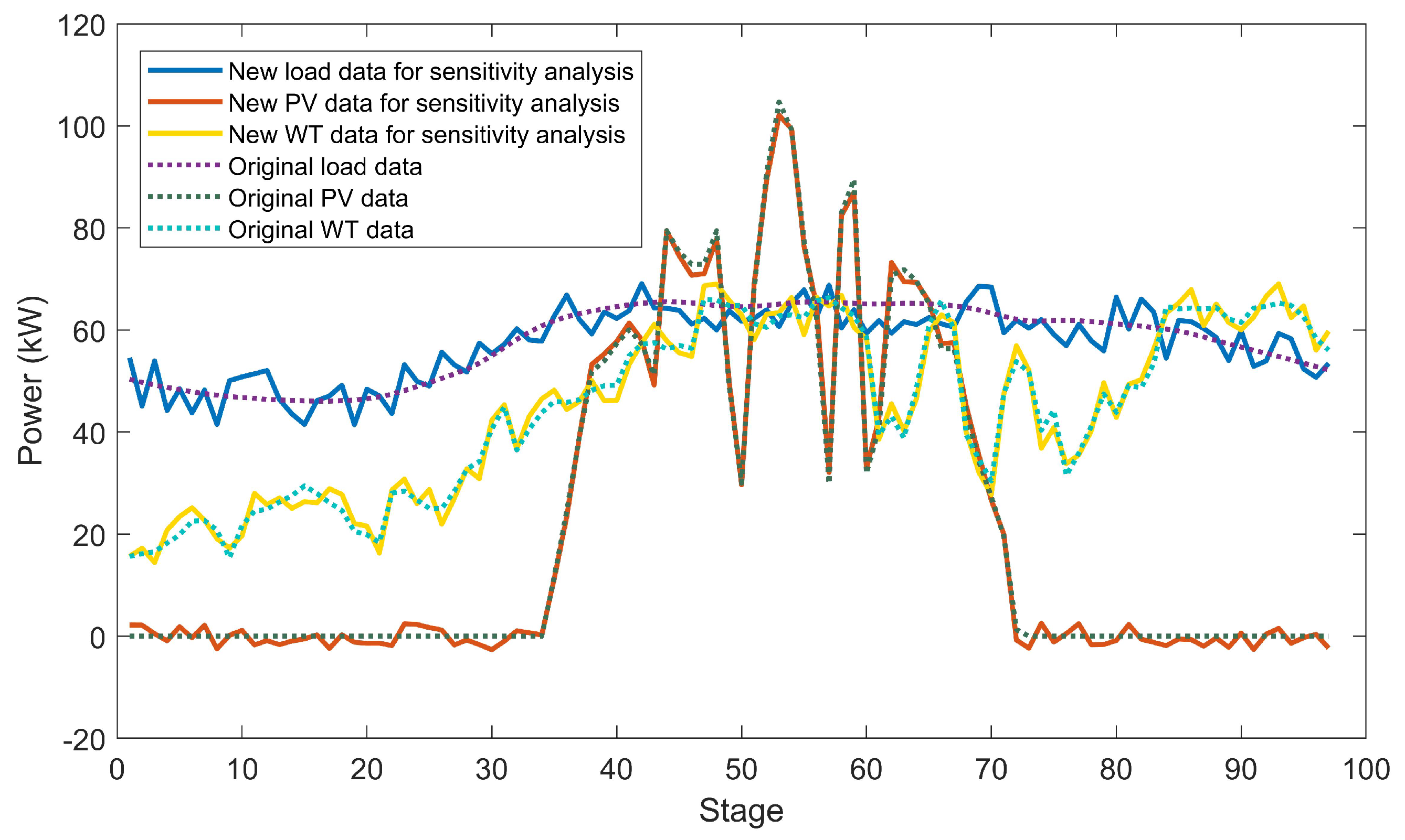
The discrete time step is still 15 min. Every single point in the original data sequence is changed by a random variation. Here, we conduct two groups of sensitivity analyses and set the variation level to 5% and 10% of the mean value of the original data. Figure 14 and Figure 15 show the new power data of load, PV generation and WT generation in one of the random cases using 5% and 10% variations, respectively. The solid curves are the new data and the dotted curves are the original data for comparison. It can be observed that the new data have higher volatility.
The result of each simulation is different since the new data are generated randomly, so we repeat the simulations many times and calculate the average economic performance for analysis. The robust method and the deterministic MPC-based method are also simulated for comparison. Corresponding results using the new input data with different variations are shown in Table 4. It can be seen that the results do not significantly change due to variations in the input data even if the actual data of load demand and RES generation are more volatile. Therefore, our proposed method is not sensitive to changes and the optimal control performance is consistent.
5. Conclusions and Future Work
In this paper, a hybrid method that combines scenario-selected optimization and reserve strategy was proposed to achieve a balanced trade-off between the reliability and efficiency of the microgrid system with interval predictions. In this method, an appropriate scenario is selected by the optimizer at each optimization step, and the optimal reservation of system capacity is determined based on the selected scenario and the possible variations in the future. The MPC method is also applied as the optimization framework to consider system dynamics in the longer term.
Simulations are conducted to compare with the existing robust method and the optimization with perfect information. Results show that our proposed method could significantly reduce the operating cost of the microgrid system while guaranteeing certain capabilities of the system to cope with the uncertainty in consumption and renewable generation. The effect of the discount factor we introduce to the cost function is discussed and guidance for finding the optimal value of this parameter is offered. The strategy of scenario selection is also analyzed, and it is shown that our proposed method can be interpreted as a conditional robust method, which validates our proposed method.
The proposed method offers good economic performance and it does not require high accuracy of prediction. Therefore, it is also suitable to extend the method for situations where accurate prediction cannot be achieved due to the limitation on hardware devices or power consumption in addition to the isolated microgrid economic dispatch. The system only needs to bear a small amount of computational burden to generate appropriate prediction intervals, and then reasonable and economical scheduling can be implemented.
In the future, we can extend the proposed method to a microgrid in the grid-connected mode where the main grid offers dynamic pricing, and try to achieve good performance in terms of system efficiency. Moreover, the problem can be reconsidered using an improved system model, where the thermal load and corresponding generators and storages are introduced, and the storage dynamics are more complicated.
Author Contributions
Conceptualization, D.D. and L.Y.; methodology, J.C.; software, J.C.; validation, J.C. and D.D.; formal analysis, J.C. and D.D.; investigation, J.C. and D.D.; resources, L.Y. and X.C.; writing–original draft preparation, J.C.; writing—review and editing, D.D., X.C., L.Y., and S.C.; supervision, L.Y. and S.C.; project administration, D.D. and X.C.; funding acquisition, L.Y. and S.C. All authors have read and agreed to the published version of the manuscript.
Acknowledgments
This work was supported in part by Key-Area Research and Development Program of Guangdong Province Project under Grant No. 2018B030338001, Natural Science Foundation of China under Grant NSFC-61629101, Shenzhen Fundamental Research Fund under Grant No. JCYJ20170411102217994, the National Science Foundation under Grant DMS-1923142, the Open Research Fund from Shenzhen Research Institute of Big Data under Grant 2019ORF01006, the National Key R&D Program of China under Grant No. 2018YFB1800800, and Guangdong Zhujiang Project under Grant No. 2017ZT07X152.
Conflicts of Interest
The authors declare no conflict of interest.
References
- Katiraei, F.; Iravani, R.; Hatziargyriou, N.; Dimeas, A. Microgrids management. IEEE Power Energy Mag. 2008, 6, 54–65. [Google Scholar] [CrossRef]
- Chen, C.; Duan, S.; Cai, T.; Liu, B.; Hu, G. Smart energy management system for optimal microgrid economic operation. IET Renew. Power Gener. 2011, 5, 258–267. [Google Scholar] [CrossRef]
- Sortomme, E.; El-Sharkawi, M.A. Optimal Power Flow for a System of Microgrids with Controllable Loads and Battery Storage. In Proceedings of the 2009 IEEE/PES Power Systems Conference and Exposition, Seattle, WA, USA, 15–18 March 2009; pp. 1–5. [Google Scholar]
- Kayalvizhi, S.; Vinod Kumar, D.M. Load Frequency Control of an Isolated Micro Grid Using Fuzzy Adaptive Model Predictive Control. IEEE Access 2017, 5, 16241–16251. [Google Scholar] [CrossRef]
- Mayhorn, E.; Xie, L.; Butler-Purry, K. Multi-Time Scale Coordination of Distributed Energy Resources in Isolated Power Systems. IEEE Trans. Smart Grid 2017, 8, 998–1005. [Google Scholar] [CrossRef]
- Sobu, A.; Wu, G. Optimal operation planning method for isolated micro grid considering uncertainties of renewable power generations and load demand. In Proceedings of the IEEE PES Innovative Smart Grid Technologies, Seattle, WA, USA, 15–18 March 2009; pp. 1–6. [Google Scholar]
- Wan, C.; Zhao, J.; Song, Y.; Xu, Z.; Lin, J.; Hu, Z. Photovoltaic and solar power forecasting for smart grid energy management. CSEE J. Power Energy Syst. 2015, 1, 38–46. [Google Scholar] [CrossRef]
- Hatziargyriou, N.; Contaxis, G.; Matos, M.; Lopes, J.A.P.; Kariniotakis, G.; Mayer, D.; Halliday, J.; Dutton, G.; Dokopoulos, P.; Bakirtzis, A.; et al. Energy management and control of island power systems with increased penetration from renewable sources. In Proceedings of the 2002 IEEE Power Engineering Society Winter Meeting. Conference Proceedings (Cat. No.02CH37309), New York, NY, USA, 27–31 January 2002; Volume 1, pp. 335–339. [Google Scholar]
- Parisio, A.; Rikos, E.; Glielmo, L. A Model Predictive Control Approach to Microgrid Operation Optimization. IEEE Trans. Control. Syst. Technol. 2014, 22, 1813–1827. [Google Scholar] [CrossRef]
- Gu, W.; Wang, Z.; Wu, Z.; Luo, Z.; Tang, Y.; Wang, J. An Online Optimal Dispatch Schedule for CCHP Microgrids Based on Model Predictive Control. IEEE Trans. Smart Grid 2017, 8, 2332–2342. [Google Scholar] [CrossRef]
- Dellino, G.; Laudadio, T.; Mari, R.; Mastronardi, N.; Meloni, C.; Vergura, S. Energy production forecasting in a PV plant using transfer function models. In Proceedings of the 2015 IEEE 15th International Conference on Environment and Electrical Engineering (EEEIC), Rome, Italy, 10–13 June 2015; pp. 1379–1383. [Google Scholar]
- Bruno, S.; Dellino, G.; La Scala, M.; Meloni, C. A microforecasting module for energy management in residential and tertiary buildings. Energies. 2019, 12, 1006. [Google Scholar] [CrossRef] [Green Version]
- Pinson, P.; Kariniotakis, G. Conditional Prediction Intervals of Wind Power Generation. IEEE Trans. Power Syst. 2010, 25, 1845–1856. [Google Scholar] [CrossRef] [Green Version]
- Sobri, S.; Koohi-Kamali, S.; Rahim, N.A. Solar photovoltaic generation forecasting methods: A review. Energy Convers. Manag. 2018, 156, 459–497. [Google Scholar] [CrossRef]
- Rastegar, M.; Fotuhi-Firuzabad, M.; Zareipour, H.; Moeini-Aghtaieh, M. A Probabilistic Energy Management Scheme for Renewable-Based Residential Energy Hubs. IEEE Trans. Smart Grid 2017, 8, 2217–2227. [Google Scholar] [CrossRef]
- Ma, X.; Dong, J.; Djouadi, S.M.; Nutaro, J.J.; Kuruganti, T. Stochastic control of energy efficient buildings: A semidefinite programming approach. In Proceedings of the 2015 IEEE International Conference on Smart Grid Communications (SmartGridComm), Miami, FL, USA, 2–5 November 2015; pp. 780–785. [Google Scholar]
- Kou, P.; Liang, D.; Gao, L.; Gao, F. Stochastic Coordination of Plug-In Electric Vehicles and Wind Turbines in Microgrid: A Model Predictive Control Approach. IEEE Trans. Smart Grid 2016, 7, 1537–1551. [Google Scholar] [CrossRef]
- Verrilli, F.; Parisio, A.; Glielmo, L. Stochastic model predictive control for optimal energy management of district heating power plants. In Proceedings of the 2016 IEEE 55th Conference on Decision and Control (CDC), Las Vegas, NV, USA, 12–14 December 2016; pp. 807–812. [Google Scholar]
- Olivares, D.E.; Lara, J.D.; Cañizares, C.A.; Kazerani, M. Stochastic-Predictive Energy Management System for Isolated Microgrids. IEEE Trans. Smart Grid 2015, 6, 2681–2693. [Google Scholar] [CrossRef]
- Shams, M.H.; Shahabi, M.; Khodayar, M.E. Stochastic day-ahead scheduling of multiple energy Carrier microgrids with demand response. Energy 2018, 155, 326–338. [Google Scholar] [CrossRef]
- Bludszuweit, H.; Dominguez-Navarro, J.A.; Llombart, A. Statistical Analysis of Wind Power Forecast Error. IEEE Trans. Power Syst. 2008, 23, 983–991. [Google Scholar] [CrossRef]
- Ai, X.; Wen, J.; Wu, T.; Lee, W. A Discrete Point Estimate Method for Probabilistic Load Flow Based on the Measured Data of Wind Power. IEEE Trans. Ind. Appl. 2013, 49, 2244–2252. [Google Scholar] [CrossRef]
- Wytock, M.; Moehle, N.; Boyd, S. Dynamic energy management with scenario-based robust MPC. In Proceedings of the 2017 American Control Conference (ACC), Seattle, WA, USA, 24–26 May 2017; pp. 2042–2047. [Google Scholar]
- Li, Y.; Wang, P.; Gooi, H.B.; Ye, J.; Wu, L. Multi-Objective Optimal Dispatch of Microgrid Under Uncertainties via Interval Optimization. IEEE Trans. Smart Grid 2019, 10, 2046–2058. [Google Scholar] [CrossRef]
- Sáez, D.; Ávila, F.; Olivares, D.; Cañizares, C.; Marín, L. Fuzzy Prediction Interval Models for Forecasting Renewable Resources and Loads in Microgrids. IEEE Trans. Smart Grid 2015, 6, 548–556. [Google Scholar] [CrossRef] [Green Version]
- Valencia, F.; Sáez, D.; Collado, J.; Ávila, F.; Marquez, A.; Espinosa, J.J. Robust Energy Management System Based on Interval Fuzzy Models. IEEE Trans. Control. Syst. Technol. 2016, 24, 140–157. [Google Scholar] [CrossRef]
- Cartagena, O.; Muñoz-Carpintero, D.; Sáez, D. A Robust Predictive Control Strategy for Building HVAC Systems Based on Interval Fuzzy Models. In Proceedings of the 2018 IEEE International Conference on Fuzzy Systems (FUZZ-IEEE), Rio de Janeiro, Brazil, 8–13 July 2018; pp. 1–8. [Google Scholar]
- Pekaslan, D.; Wagner, C.; Garibaldi, J.M.; Marin, L.G.; Sáez, D. Uncertainty-Aware Forecasting of Renewable Energy Sources. In Proceedings of the 2020 IEEE International Conference on Big Data and Smart Computing (BigComp), Busan, Korea, 19–22 February 2020; pp. 240–246. [Google Scholar]
- Rafiei, M.; Niknam, T.; Aghaei, J.; Shafie-Khah, M.; Catalão, J.P.S. Probabilistic Load Forecasting Using an Improved Wavelet Neural Network Trained by Generalized Extreme Learning Machine. IEEE Trans. Smart Grid 2018, 9, 6961–6971. [Google Scholar] [CrossRef]
- Marín, L.G.; Cruz, N.; Sáez, D.; Sumner, M.; Núñez, A. Prediction interval methodology based on fuzzy numbers and its extension to fuzzy systems and neural networks. Expert Syst. Appl. 2019, 119, 128–141. [Google Scholar] [CrossRef] [Green Version]
- Mohan, V.; Suresh, R.; Singh, J.G.; Ongsakul, W.; Madhu, N. Microgrid Energy Management Combining Sensitivities, Interval and Probabilistic Uncertainties of Renewable Generation and Loads. IEEE J. Emerg. Sel. Top. Circuits Syst. 2017, 7, 262–270. [Google Scholar] [CrossRef]
- Vandoorn, T.L.; Vasquez, J.C.; De Kooning, J.; Guerrero, J.M.; Vandevelde, L. Microgrids: Hierarchical Control and an Overview of the Control and Reserve Management Strategies. IEEE Ind. Electron. Mag. 2013, 7, 42–55. [Google Scholar] [CrossRef] [Green Version]
- Vandoorn, D.Q.; Rawlings, J.B.; Rao, C.V.; Scokaert, P.O.M. Constrained model predictive control: Optimality and stability. Automatica 2000, 36, 789–814. [Google Scholar]
- Palma-Behnke, R.; Benavides, C.; Lanas, F.; Severino, B.; Reyes, L.; Llanos, J.; Sáez, D. A Microgrid Energy Management System Based on the Rolling Horizon Strategy. IEEE Trans. Smart Grid 2013, 4, 996–1006. [Google Scholar] [CrossRef] [Green Version]
- Xiang, Y.; Liu, J.; Liu, Y. Robust Energy Management of Microgrid With Uncertain Renewable Generation and Load. IEEE Trans. Smart Grid 2016, 7, 1034–1043. [Google Scholar] [CrossRef]
- Sheng, H.; Xiao, J.; Cheng, Y.; Ni, Q.; Wang, S. Short-Term Solar Power Forecasting Based on Weighted Gaussian Process Regression. IEEE Trans. Ind. Electron. 2018, 65, 300–308. [Google Scholar] [CrossRef]
- Griva, I.; Nash, S.G.; Sofer, A. Linear and Nonlinear Optimization; SIAM: Philadelphia, PA, USA, 2009; pp. 149–162. [Google Scholar]
- Li, Z.; Zang, C.; Zeng, P.; Yu, H.; Li, S. Fully Distributed Hierarchical Control of Parallel Grid-Supporting Inverters in Islanded AC Microgrids. IEEE Trans. Ind. Inform. 2018, 14, 679–690. [Google Scholar] [CrossRef]
- Bevrani, H. Robust Power System Frequency Control; Springer: New York, NY, USA, 2009; pp. 19–37. [Google Scholar]
- Bidram, A.; Davoudi, A. Hierarchical Structure of Microgrids Control System. IEEE Trans. Smart Grid 2012, 3, 1963–1976. [Google Scholar] [CrossRef]
- Morstyn, T.; Hredzak, B.; Agelidis, V.G. Control Strategies for Microgrids With Distributed Energy Storage Systems: An Overview. IEEE Trans. Smart Grid 2018, 9, 3652–3666. [Google Scholar] [CrossRef] [Green Version]
- Han, Y.; Li, H.; Shen, P.; Coelho, E.A.A.; Guerrero, J.M. Review of Active and Reactive Power Sharing Strategies in Hierarchical Controlled Microgrids. IEEE Trans. Power Electron. 2017, 32, 2427–2451. [Google Scholar] [CrossRef] [Green Version]
- Moehle, E.N. Busseti, S.B.; Wytock, M. Dynamic energy management. Arxiv 2019, arXiv:1903.06230. [Google Scholar]
- Bertsekas, D.P. Dynamic Programming and Optimal Control; Athena Scientific: Nashua, NH, USA, 1995; pp. 402–445. [Google Scholar]
- Venayagamoorthy, G.K.; Sharma, R.K.; Gautam, P.K.; Ahmadi, A. Dynamic Energy Management System for a Smart Microgrid. IEEE Trans. Neural Netw. Learn. Syst. 2016, 1, 1643–1656. [Google Scholar] [CrossRef]
- Floudas, C. Nonlinear and Mixed-Integer Optimization: Fundamentals and Applications; Oxford University Press: Oxford, UK, 1995. [Google Scholar]
- Bulut, A.; Ralphs, T.K. On the complexity of inverse mixed integer linear optimization. In Technical Report 15T-001-R3; Lehigh University: Bethlehem, PA, USA, October 2016. [Google Scholar]
- Richards, A.; How, J. Mixed-integer programming for control. In Proceedings of the 2005 American Control Conference, Portland, OR, USA, 8–10 June 2005; Volume 4, pp. 2676–2683. [Google Scholar]
- Padberg, M.; Rinaldi, G. A branch-and-cut algorithm for the resolution of large-scale symmetric traveling salesman problems. SIAM Rev. 1991, 33, 60–100. [Google Scholar] [CrossRef]
- Streiffert, D.; Philbrick, R.; Ott, A. A mixed integer programming solution for market clearing and reliability analysis. In Proceedings of the IEEE Power Engineering Society General Meeting, San Francisco, CA, USA, 16 June 2005; Volume 3, pp. 2724–2731. [Google Scholar]
- Chen, Y.; Casto, A.; Wang, F.; Wang, Q.; Wang, X.; Wan, J. Improving Large Scale Day-Ahead Security Constrained Unit Commitment Performance. IEEE Trans. Power Syst. 2016, 31, 4732–4743. [Google Scholar] [CrossRef]
- Achterberg, T.; Wunderling, R. Mixed integer programming: Analyzing 12 years of progress. Facet. Comb. Optim. 2013, 31, 449–481. [Google Scholar]
- Gurobi Optimization Inc. Algorithms in Gurobi. 2016. Available online: https://www.gurobi.com/pdfs/user-events/2016-frankfurt/Die-Algorithmen.pdf (accessed on 20 May 2020).
- Löfberg, J. YALMIP: A Toolbox for Modeling and Optimization in MATLAB. In Proceedings of the 2004 IEEE International Conference on Robotics and Automation (IEEE Cat. No.04CH37508), New Orleans, LA, USA, 2–4 September 2004; pp. 284–289. [Google Scholar]
- Gurobi Optimization Inc. Gurobi Optimizer Reference Manual. 2014. Available online: http://www.gurobi.com (accessed on 29 July 2019).
- Gurobi Optimization Inc. Mixed-Integer Programming (MIP) – A Primer on the Basics. 2014. Available online: https://www.gurobi.com/resource/mip-basics/ (accessed on 20 May 2020).
- Luna-Rubio, R.; Trejo-Perea, M.; Vargas-Vázquez, D.; Ríos-Moreno, G.J. Optimal sizing of renewable hybrids energy systems: A review of methodologies. Sol. Energy 2012, 86, 1077–1088. [Google Scholar] [CrossRef]
- Raimondi Cominesi, S.; Farina, M.; Giulioni, L.; Picasso, B.; Scattolini, R. A Two-Layer Stochastic Model Predictive Control Scheme for Microgrids. IEEE Trans. Control. Syst. Technol. 2018, 26, 1–13. [Google Scholar] [CrossRef]
- Garcia, C.E.; Prett, D.M.; Morari, M. Model predictive control: theory and practice—A survey. Automatica 1989, 25, 335–348. [Google Scholar] [CrossRef]
Figure 1.
System model of the isolated microgrid.

Figure 2.
Hierarchical microgrid control model.

Figure 3.
Actual power data of load, PV and wind turbine in 48 h.

Figure 4.
Operation results using our proposed method based on MPC.

Figure 5.
Charging/discharging power and reserve power of battery in the dispatch stage using our proposed method.
Figure 5.
Charging/discharging power and reserve power of battery in the dispatch stage using our proposed method.

Figure 6.
Charging/discharging power and reserve power of battery in the operation stage using our proposed method.
Figure 6.
Charging/discharging power and reserve power of battery in the operation stage using our proposed method.

Figure 7.
Operation results using an existing robust method.

Figure 8.
Dispatch cost of our proposed method and the robust method.

Figure 9.
Operation cost of our proposed method and the robust method.

Figure 10.
Operation cost of our proposed method, existing robust method, and MPC-based optimization method with different .
Figure 10.
Operation cost of our proposed method, existing robust method, and MPC-based optimization method with different .

Figure 11.
Scenarios selected by optimizer.

Figure 12.
Scenarios selected by optimizer (zoomed in).

Figure 13.
Simulation results related to the reserve strategy. Top: the power differences of RES generation and load demand. Middle: the reserve level over stages. Bottom: the reserve powers in battery and DGs.
Figure 13.
Simulation results related to the reserve strategy. Top: the power differences of RES generation and load demand. Middle: the reserve level over stages. Bottom: the reserve powers in battery and DGs.

Figure 14.
Actual power data with 5% variation and the original power data of load, PV, and WT in one day.
Figure 14.
Actual power data with 5% variation and the original power data of load, PV, and WT in one day.

Figure 15.
Actual power data with 10% variation and the original power data of load, PV, and WT in one day.
Figure 15.
Actual power data with 10% variation and the original power data of load, PV, and WT in one day.


Table 1.
Simulation parameters.
| Discrete time step | 15 [min] |
| Duration of simulation | 24 [h] |
| Total operation steps | 96 |
| Horizon of MPC methodM | 24 [h] |
Table 2.
Average economic performances
| Method | Dispatch Cost | Operation Cost |
|---|---|---|
| Our proposed method | 960.74 | 1246.2 |
| Existing robust method | 1262.9 | 1355.0 |
| MPC-based optimization method | 1218.3 | 1340.7 |
Table 3.
Operation cost versus .
| Method | Our Proposed Method | Existing Robust Method | MPC-Based Optimization Method |
|---|---|---|---|
| = 1 | 1344.8 | 1355.0 | 1340.7 |
| = 0.9 | 1315.0 | 1442.8 | 1331.4 |
| = 0.8 | 1246.2 | 1390.6 | 1332.5 |
| = 0.7 | 1314.7 * | 1588.6 * | 1540.4 |
* The value of is too small that inevitable violations occur in the simulations of our method and the robust method, so here we only use the smallest costs for comparison.
Table 4.
Average economic performances using new data with 5% and 10% variation.
| Method | Our Proposed Method | Existing Robust Method | MPC-Based Optimization Method | |
|---|---|---|---|---|
| 5% Variation | Dispatch Cost | 915.08 | 1250.5 | 1215.2 |
| Operation Cost | 1241.6 | 1365.3 | 1334.4 | |
| 10% Variation | Dispatch Cost | 960.96 | 1232.8 | 1209.3 |
| Operation Cost | 1249.1 | 1338.8 | 1321.2 | |
© 2020 by the authors. Licensee MDPI, Basel, Switzerland. This article is an open access article distributed under the terms and conditions of the Creative Commons Attribution (CC BY) license (http://creativecommons.org/licenses/by/4.0/).
Share and Cite
MDPI and ACS Style
Cheng, J.; Duan, D.; Cheng, X.; Yang, L.; Cui, S. Probabilistic Microgrid Energy Management with Interval Predictions. Energies 2020, 13, 3116. https://doi.org/10.3390/en13123116
AMA Style
Cheng J, Duan D, Cheng X, Yang L, Cui S. Probabilistic Microgrid Energy Management with Interval Predictions. Energies. 2020; 13(12):3116. https://doi.org/10.3390/en13123116
Chicago/Turabian StyleCheng, Jiayu, Dongliang Duan, Xiang Cheng, Liuqing Yang, and Shuguang Cui. 2020. "Probabilistic Microgrid Energy Management with Interval Predictions" Energies 13, no. 12: 3116. https://doi.org/10.3390/en13123116
Note that from the first issue of 2016, this journal uses article numbers instead of page numbers. See further details here.