Optimized Placement of Onshore Wind Farms Considering Topography

Abstract

As the scale of onshore wind farms are increasing, the influence of wake behavior on power production becomes increasingly significant. Wind turbines sittings in onshore wind farms should take terrain into consideration including height change and slope curvature. However, optimized wind turbine (WT) placement for onshore wind farms considering both topographic amplitude and wake interaction is realistic. In this paper, an approach for optimized placement of onshore wind farms considering the topography as well as the wake effect is proposed. Based on minimizing the levelized production cost (LPC), the placement of WTs was optimized considering topography and the effect of this on WTs interactions. The results indicated that the proposed method was effective for finding the optimized layout for uneven onshore wind farms. The optimization method is applicable for optimized placement of onshore wind farms and can be extended to different topographic conditions.

1. Introduction

With the high recent demand for clean energy, wind energy has become increasingly important because of its many advantages, such as environmental friendliness, safety, and also high utilization. According to the Global Wind Energy Council (GWEC) 2018, the worldwide newly installed capacity of wind energy will exceed 60 GW in 2020, distributed over about 100 countries, and it is estimated that the globally installed wind energy capacity will exceed 800 GW [1].

The wake effect is a phenomenon where the wind turbine (WT) draws energy from the wind and forms a wake where the wind velocity of downstream WT is reduced [2]. If the downstream WT is in the wake, the wind speed of the downstream WT is lower than the wind speed of the upstream WT and the wake effect causes an uneven distribution of wind power and a decline in production. The wake effect results in energy losses which reduce the annual energy production by about 10–15%, causing great financial losses to wind farm owners [3]. Due to the gradually advanced wind power technology, more and more large-scale wind farms have been built and the wake losses have become more evident at the same time. This also affects the WTs control strategy and operating reserve [4,5]. To estimate the wind velocity arriving at the downstream WT through the upstream WT, there are several popular and accurate wake models nowadays [6]. Among them, the Jensen model is based on momentum conservation theory and proposes that wake flow should be assumed to expand linearly after downstream WTs [7]. A two-dimensional parabolic model and a semi-analytical wake model were proposed by Ainslie [8] and Larsen [9], respectively. For the sake of precision, computational fluid dynamics (CFD) technology considering dynamic wake behavior is an optional approach to estimate the wake effect for more accurate results [10].

One of the main factors in determining the placement of wind turbines within a wind farm is the wake effect among WTs. The problem of wind farm layout optimization is to minimize the wake losses as well as keeping down construction costs by optimizing the location of the WT. In 1994, Mosetti et al. [11] completed the first true wind farm layout optimization using genetic algorithms. After that, References [12,13] proved the superiority of their respective method to get more power production or to reduce optimization time compared with the first trial. Due to the small impact of the offshore wind farm on the environment and the rich wind resources, some wind farm optimization efforts are imposed on offshore wind farms [14,15,16]. For example, the land carrying capacity, WT hub height, seabed conditions and many other practical aspects are considered for WT placement in a wind farm [14]. In Reference [15], the WT sittings of a wind farm are optimized aimed at minimal LPC within spare spacings. Similarly, wind farm layout optimization in Reference [16] takes restricted areas into account. There are restrictions on the shape of wind farms such as natural gas pipelines and oil wells. Because of excessive investment, climate limitations, and maintenance difficulties of offshore wind farms compared to onshore wind farms, onshore wind farms are also attracting increasing attention from wind power companies. Therefore, onshore wind farm owners need to evaluate wake effects based on the influence of topographic height due to uneven terrain conditions. There are some researches related to the topography of wind farms. A comprehensive study about some wake models with constant or variable turbine hub heights is presented in Reference [17], but it does not discuss the layout optimization. After that, a detailed analysis and optimization of hub height of WTs can be seen in Reference [18]. For reducing the wake effect, a detailed analysis of adjustment of hub height is carried out, and the optimization for variable hub heights between upstream WTs and downstream WTs also can be found. However, the optimization work in Reference [18] is aimed at the hub height adjustment considering the friction of the ground, etc., rather than the influence of natural topographic conditions on the layout. More importantly, the only optimization parameter is the hub height, not the locations of WTs. In previous research works, some did not carry out optimization work, and some optimization work mainly focused on other variables such as the hub height, rather than the problem of optimizing WT layout. In addition, studies about the terrain issue of wind farms are also reflected in References [19,20], both of which use CFD techniques to evaluate the wake effect of wind farms. Although this fluid dynamics approach will make the results more accurate in the case of terrain, the calculation process for CFD takes too much time and is not as convenient for the next step of optimization as the analytical wake model [10].

The typical feature of onshore wind farms compared to offshore wind farms is the terrain issue. This paper proposes an optimization methodology for three-dimensional onshore wind farms to find the optimized WTs placement. It extends existing work by focusing on variations in topography of the ground above sea level, and the effect of this on WT interactions. Then the developed model is used to optimize the LPC compared with a reference layout wind farm. And it is a meaningful contribution to optimize the WTs layout as an optimization parameter for three-dimensional onshore wind farms considering topography combined with wake effect.

In this paper, topographic height refers to topography above sea level. The mathematical equations for wake model and energy model considering topography are specified in Section 2. The objective is presented in Section 3. In Section 4, the theory and method of the evolution algorithm PSO for the non-linear problem and the optimization framework are discussed. Simulation results and analysis are presented in Section 5. Finally, the conclusion is given in Section 6.

2. System Models

In this section, the Jensen wake model is adopted to propose a wake model which takes wake effect and topography into consideration for onshore wind farms. After that, the energy model of onshore wind farms is presented.

2.1. Wake Model

The Jensen wake model is a commonly used analytical wake model and it is here chosen as the basis of the development of 3D wake model due to its effectiveness and simplicity. The wind velocity of the x-th downstream WT caused by one upstream WT is calculated as [21]:

$$V_x=V_0-V_0(1-\sqrt{1-C_T}){\left(\frac{R_0}{R_x}\right)}^2\left(\frac{S_{overlap}}{S_0}\right)$$

(1)

where C_T is a thrust coefficient for the WT, V₀ is the initial velocity at upstream WT, and S_overlap is the actual overlap area between wake area and downstream blade sweeping area S₀. Then R_x is the wake radius generated by linear expansion of WT radius R₀ with the distance x between upstream and downstream WT.

$$R_x=R_0+kx$$

(2)

where k is the wake decay constant valued 0.07 for onshore wind farms [22].

2.2. Combination of Wake

There is a phenomenon called wake combination where one downstream WT is not only affected by one upstream WTs in the wind farm. The method to estimate the problem has been proposed by Katic et al. [6] using the sum of squares of velocity deficits. Then, the wind velocity at the x-th downstream WT caused by N WTs can be calculated as:

$$V_y=V\left[1-\sqrt{{\displaystyle \sum _{y=1}^N\left[1-\left(\frac{V_x}{V_0}\right)\right]}}\right]$$

(3)

2.3. Wind Shear

Wind shear can be explained that the wind velocity changes with heights [22]. With increased height, wind velocity increases in the near-surface layer. This effect should be considered when the onshore wind farm is built on uneven terrain. The equation of the updated wind velocity is shown as:

$$V_{xy}=V_0\frac{\ln \left(\frac{z_{\mathrm{xy}}}{h_0}\right)}{\ln \left(\frac{z_{ref}}{h_0}\right)}$$

(4)

where z_xy is the actual height, and z_ref shows the reference height, and h₀ is the surface roughness.

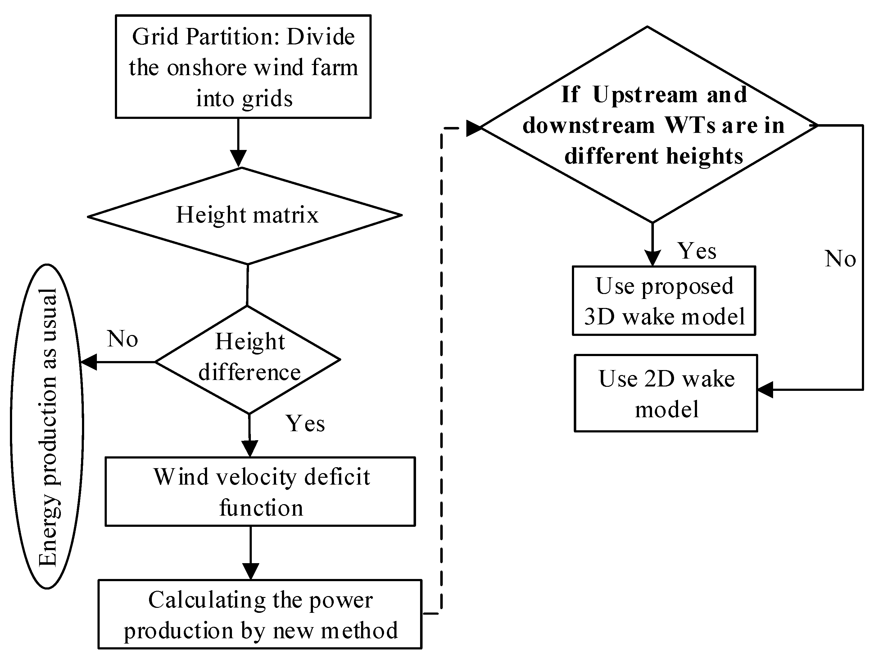
2.4. Wake Model for Different Topographic Heights

When the WTs are on flat ground, the center of the wake area generated by the wake effect of the upstream WT will be on the same level as the center of the downstream blade swept area of the downstream one. The wake flow generated by the upstream WT imposed on the downstream one is shown as a circle consisting of purple and red in Figure 1. However, when there is a difference in topography, the center of the blade swept area will be shifted upward by the same distance as the height difference between the upstream and downstream WTs, as shown by the blue and red circles in the Figure 1. The shift makes the distance between the centers of the swept areas more separate and then the area of overlap of the downstream rotor’s swept area with the upstream rotor’s wake is decreased.

If the onshore wind farm is constructed in a zone with different heights, the wind velocity at the downstream WT is affected by

(1) the wind shear effect

As Equation (4) shows, the wind speed will increase slightly with the elevation of the air.

(2) the wake effect from upstream wind turbines

And the wake effect from upstream wind turbines needs to take the relative topographical difference into account as the wake is modelled as a (truncated) cone in three dimensions, subjecting to wind direction and other turbines.

The wind direction is facing the wind turbine in the case of Figure 1, and if the wind direction changes, the description and corresponding model will be as presented below.

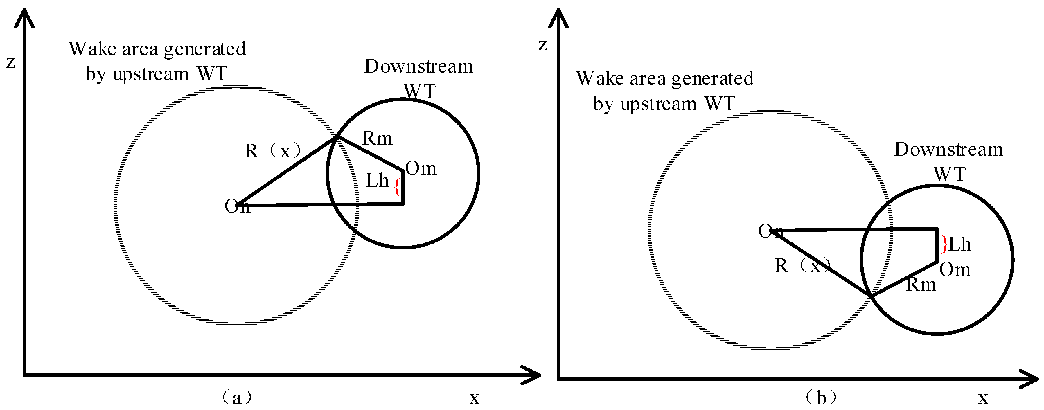
The downstream WT in different topographic height are affected partially by the wake generated by the upstream WT. If both the upstream and the downstream WT are at the same topographic height, which means the circle centers are also at the same height, the wake effect area is unchanged. If the WTs are not at the same topographic height then there are two cases, where the affected wake area will be reduced because of the different height of topography L_h as illustrated in Figure 2a,b.

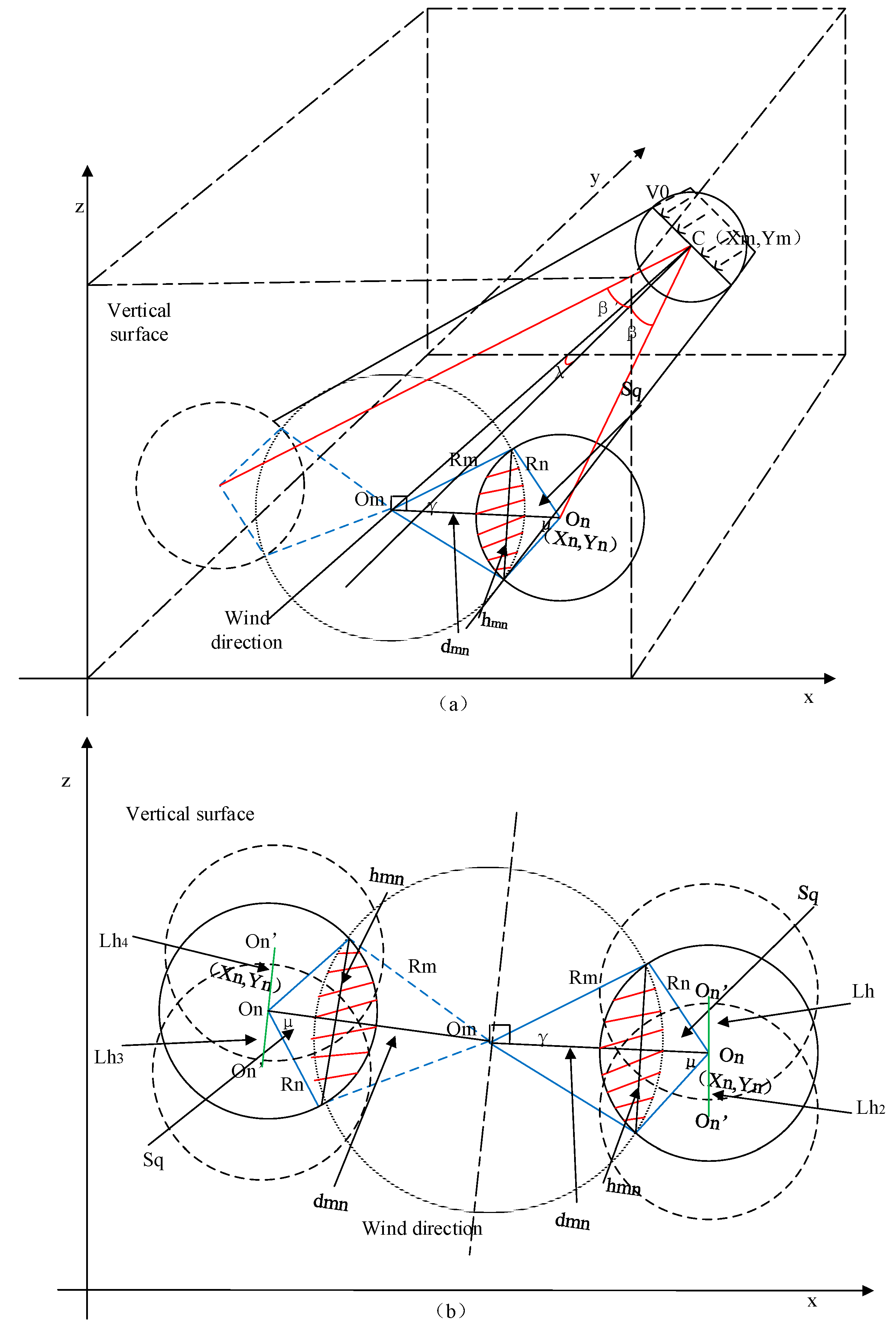
In this model, the two cases corresponding to Figure 2 need to be analyzed in details as illustrated in Figure 3. The extra circles are used for expressing the state of moving up and down, left and right in Figure 3. The solid circle represents the wake area of the upstream WT in the downstream moving left and right, and the dotted circle represents the changes in height of the wake area moving up and down based on the solid circle. If the WTs are at the same height, a two-dimensional model will be chosen to calculate the power production of onshore wind farms as shown in Figure 3a. The vertical z–x plane portion of Figure 3b is the same as that of Figure 3a. Only the z–x plane is selected for illustration and analysis to make it more intuitive, where the z-axis represents translation in the z-direction due to changes in terrain height. Hence, the blue line L_mn is the interval between the center of the upstream WT and the downstream one. The overlapping areas are indicated as the shaded area as Overlap. The blue quadrangle area is denoted as S_q. While the new version of 3D wake model by taking the topographic height difference’s impact on the wake area into consideration, the related analyses are shown in Figure 3b.

The 2D wake model is shown in Figure 3a while Figure 3b dotted circles refer to the proposed model. When the wake area generated by the upstream WT is as shown in the solid circle on the right side of Figure 3a, some equations can be derived as Equations (5)–(15).

$$L_{mn}=\sqrt{{\left(x_n-x_m\right)}^2+{\left(y_n-y_m\right)}^2}$$

(5)

$$L_h=O_n{O}_n{}^{\prime }=d_y\cdot \sin \alpha$$

(6)

$${\mathrm{d}}_{mn}=\sqrt{{\left(L_{mn}\left|\sin \left(\beta +\lambda \right)\right|\right)}^2+{\left(L_h\right)}^2}$$

(7)

$$R_n=R_m+k{L}_{mn}\left|\cos \left(\beta +\lambda \right)\right|$$

(8)

$$\mu =2{\cos }^{-1}\frac{R_n{}^2+d_{mn}{}^2-R_m{}^2}{2R_n{d}_{mn}}$$

(9)

$$\gamma =2{\cos }^{-1}\frac{R_m{}^2+d_{mn}{}^2-R_n{}^2}{2R_m{d}_{mn}}$$

(10)

$$h_{mn}=2R_m\left|\sin \left(\mu /2\right)\right|$$

(11)

$$S_m=\gamma \frac{R_m{}^2}{2}$$

(12)

$$S_n=\mu \frac{R_n^2}{2}$$

(13)

$$S_q=\frac{h_{mn}{d}_{mn}}{2}$$

(14)

$$S_{overlap}=S_m+S_n-S_q$$

(15)

The L_mn is the distance between upstream and downstream WTs, and the d_y is the y-axis optimized distance among WTs. The wind speed at row x, column y can be calculated as Equation (16). The overlapping area S_overlap is calculated by the area of the sector circle with a radius of R_m and a chord angle of μ plus the area of the sector circle with a radius of R_n and a chord angle of λ, then minus the rectangular area of the blue side in the Figure 3. All geometrical other variables are defined in Figure 3a,b.

So, the S_overlap of Equation (1) should be adjusted as given by the above calculations:

$$V_x=V_0\left[1-\left(1-\sqrt{1-C_{T,mn}}\right){\left(\frac{R_0}{R_x}\right)}^2\left(\frac{S_{overlap}^{\prime }}{S_0}\right)\right]$$

(16)

When the wake area is located on the other side in Figure 3a, the corresponding formula can be obtained by changing all (β + λ) to (β − λ) without changing other parts. It is worth noting that wake analyses above are steady-state cases and the wake center moves up and down and left and right during operation, but it averages around a certain position. However, the overlap will change with the wind direction.

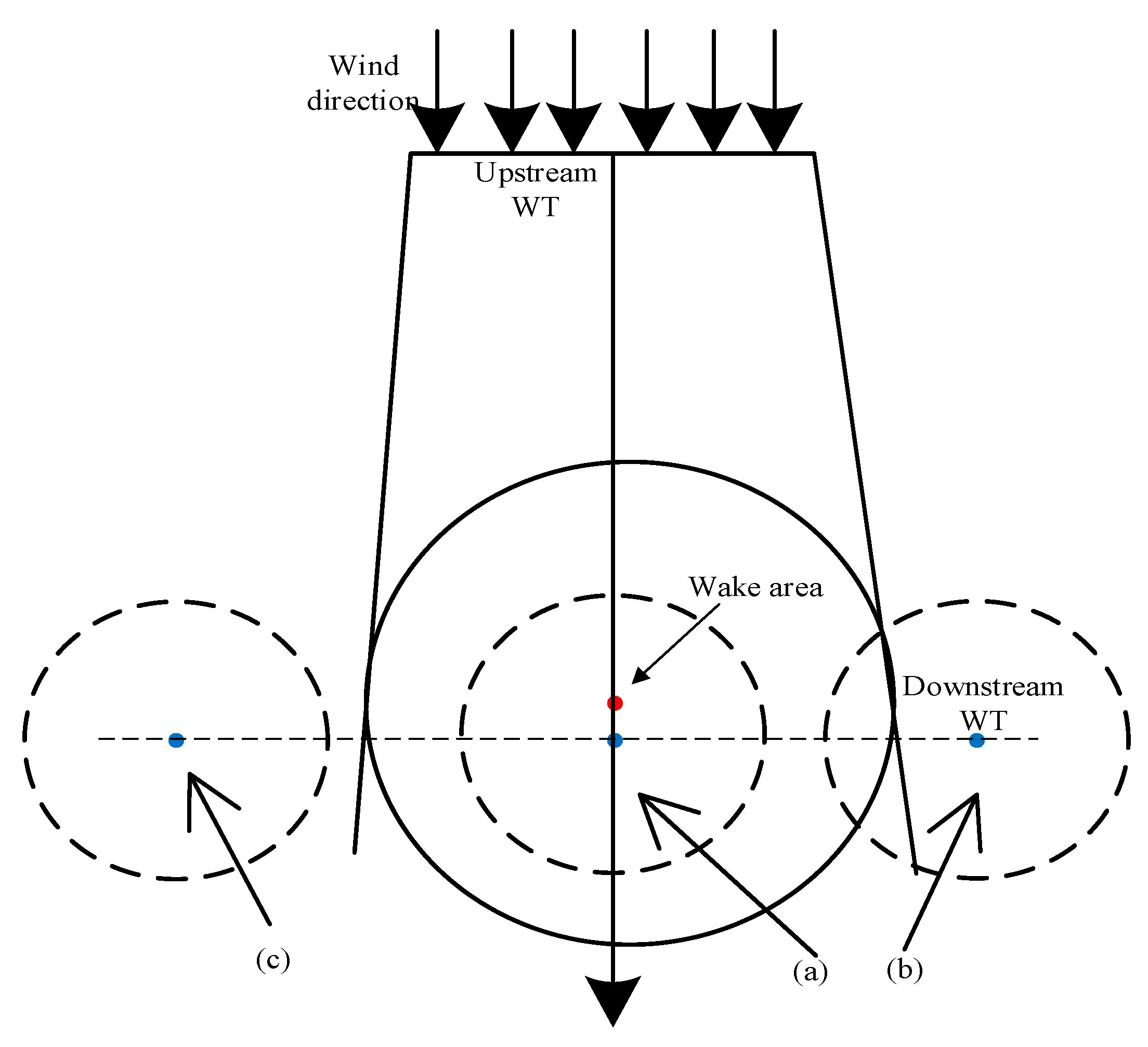
In Figure 4, the location of the downstream WT is indicated by the dotted circle. The solid, red dot represents the center of the solid circle, and the solid circle is the wake area generated by the upstream WT. The solid, blue dot represents the center of the dotted circle and the dotted circle is the downstream WT blade sweeping area. The wake effect will be receded gradually if the downwind WT is moving from position (a) to (c). The mathematical criterion reference for three conditions of overlap area is shown in

Table 1. Judgement criteria.

Classification	Name	Condition	Formula
(A)	Full overlap	$0\le d_{mn}\le R_m-R_n$	(1)–(3)
(B)	Partial overlap	$R_m-R_n\le d_{mn}\le R_m+R_n$	(5)–(16)
(C)	Non-overlap	$d_{mn}\ge R_m+R_n$	$V_n=V_o$

.

2.5. Energy Model

In this paper, the power production of each WT is calculated by assuming a maximum power point tracking (MPPT) control strategy [23]. The power production of at the m-th row, the n-th column WT can be expressed using the power coefficient C_p,opt obtained from the blade pitch angle β′ and the tip speed ratio λ_opt [24,25] based on MPPT:

$$P_{mn}=0.5C_{p,opt}({\beta }^{\prime },{\lambda }_{opt})\rho \mathsf{\pi }{R}^2{V}_y^3$$

(17)

where ρ is the air density. The total power production from N_max WTs can be given as:

$$P_{tol}={\displaystyle \sum _{N=1}^{N_{\max }}{P}_N}$$

(18)

2.6. Cost Model

Due to the cost of electrical systems, typically the investment of wind farms is large. Reducing the investment while guaranteeing energy generation are a two-pronged approach. The mathematical models to estimate the cost of WTs placement design is presented. Among them, the capital investment, operating, and maintenance costs are considered in the total discounted costs during the economic lifetime. Inside, the capital investment can be obtained from the cable cost as follows [26]:

$$C_n=A_p+B_p\exp {\left(\frac{C_p{S}_n}{{10}^8}\right)}^2$$

(19)

$$S_n=\sqrt{3}{I}_{rated}{U}_{rated}$$

(20)

$$CA{P}_T={\displaystyle \sum _n^N{C}_n{L}_n}=CA{P}_T\left(L_x,L_y\right)$$

(21)

where A_p, B_p, and C_p are cost constants. The S_n, U_rated, and I_rated indicate the rated power, the rated voltage and the rated current of the cable respectively. The C_p is unit cost of cable p, while L_n is the length of cable n. The levelized production cost is adopted for the objective function, which contains the total discounted cost and the total discounted energy production. The mathematical equations of LPC for the onshore wind farm are formulated in [27].

$$C_0={\displaystyle \sum _{T=1}^{N_Y}CA{P}_T{\left(1+r\right)}^{-t}}$$

(22)

$$LPC=\left[\frac{C_0\left(L_x,L_y\right)r{\left(1+r\right)}^{N_t}}{{\left(1+r\right)}^{N_t}-1}+OA{M}_t\right]\frac{1}{E_{tol}\left(L_x,L_y\right)}$$

(23)

$$r=\frac{1+v}{1+i}-1$$

(24)

where E_out is the average annual energy production generated by the onshore wind farm. The C₀ is the total investment and is assumed to be made in the first year and paid off during the economic cycle, which relates to the bank interest rate v and the inflation rate i. The N_t is the economic cycle and OAM_t indicate the operation and maintenance cost every year.

3. Method for Calculation and Selected Objective Function

A matrix method and its framework are presented to estimate the onshore wind farm (WF) terrain height for calculating the energy production. The objective function is shown in this section.

3.1. Matrix Presentation of Topographical Data

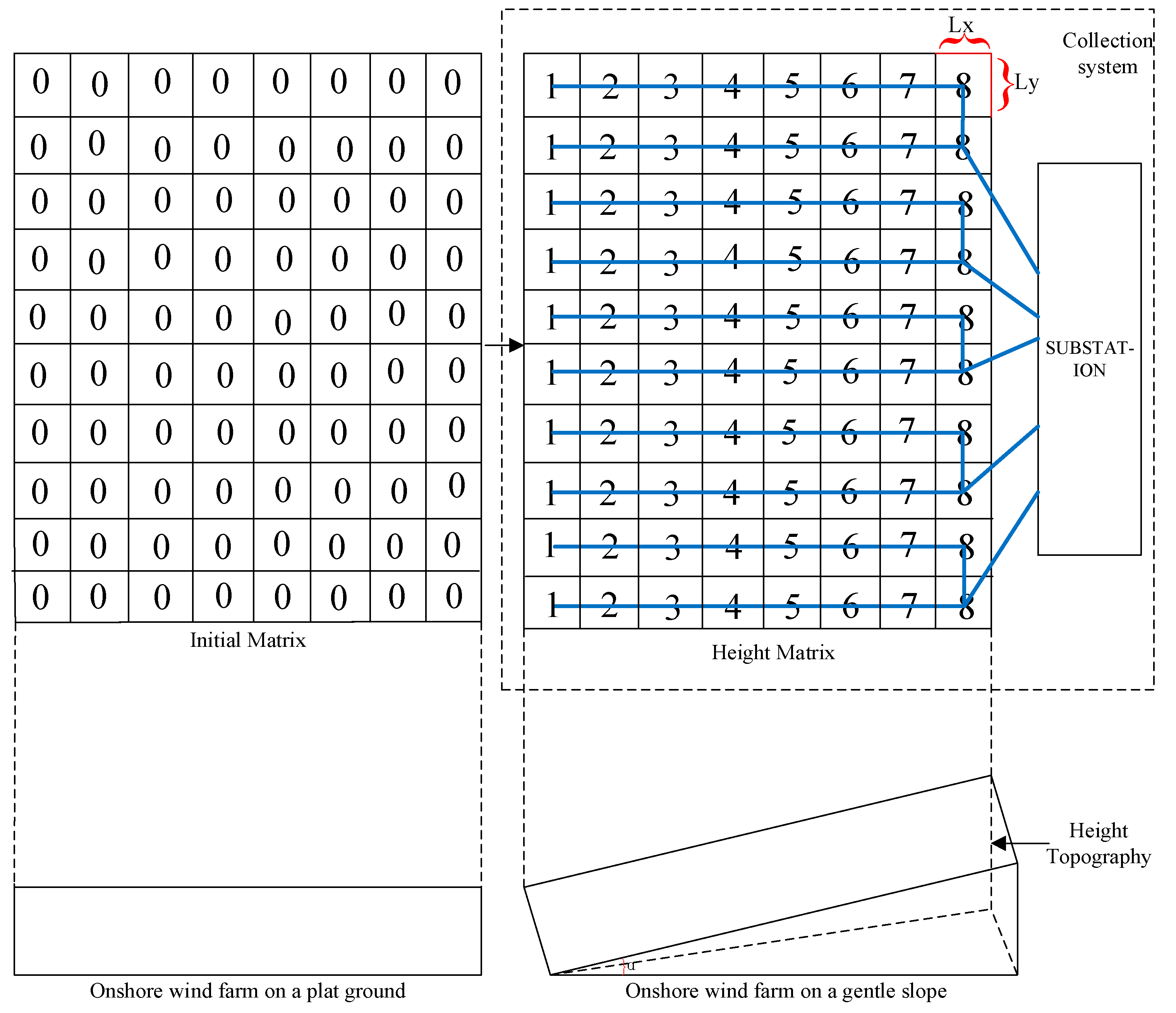
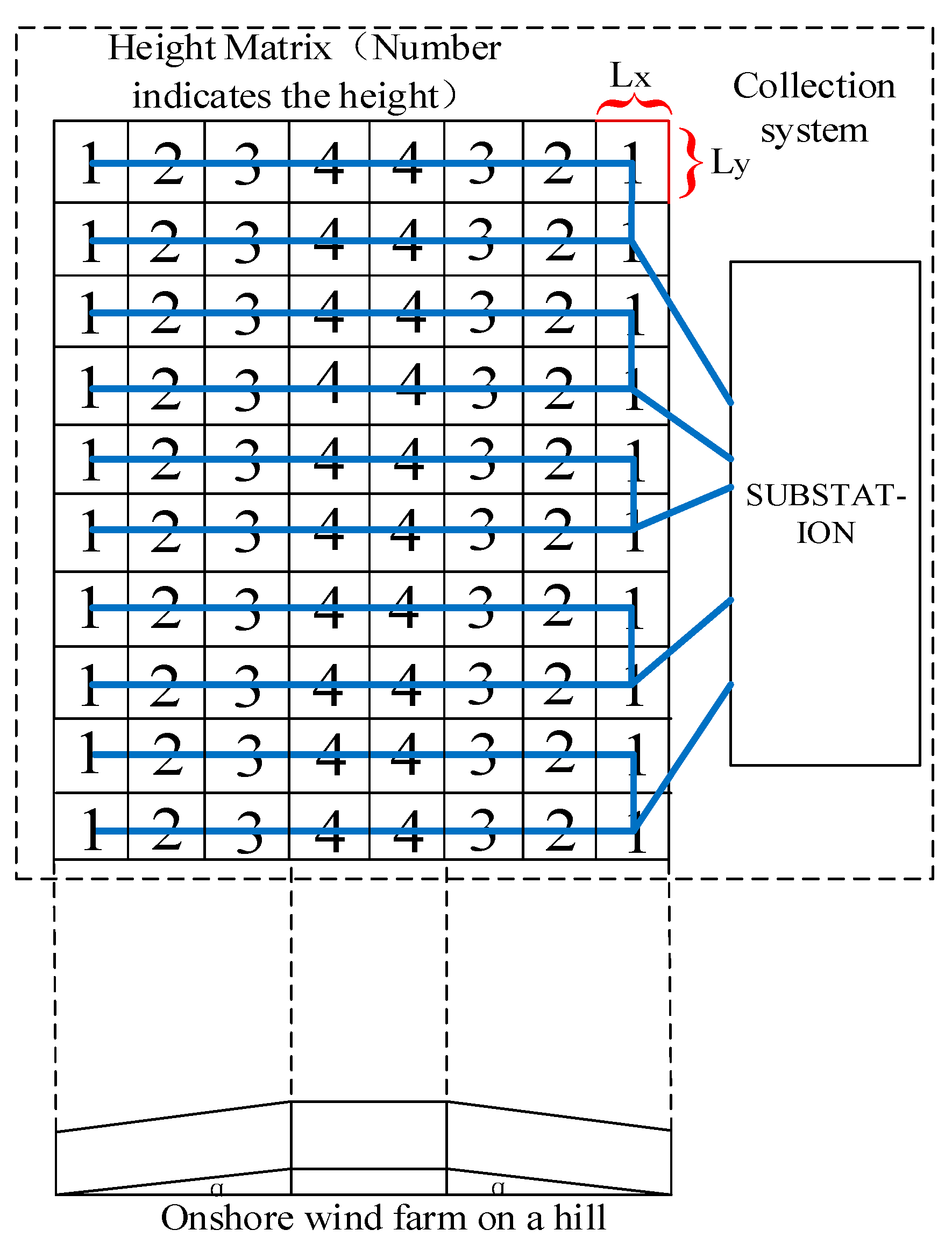
The topographical data for the optimization problem is stored in a matrix as shown in Figure 5.

The WTs are arranged in a square grid, so there is a WT in each square in the figure. The matrix holds topographical data at the base of each WT in the grid, as a ratio of the distance between adjacent WTs, so the right-hand matrix in the picture shows an increase of elevation with a α degree slope. Blue lines in the figure indicate cables used to connect the WTs.

This is called matrix H, which allows us to write topographical differences between the m-th row, the n-th column WT and the i-th row, the j-th column WT as follows:

$$L_h=\left[\left|H\left(m,n\right)-H\left(i,j\right)\right|\right]d_y\sin \alpha$$

(25)

In fact, the height difference for topography is considered and the wind speed changes because of the wind shear effect. Besides, wake area is changed due to the height difference. It is assumed that the pressure gradient and streamline distortion are not considered here, but the related research can refer to [28]. Thus, the following wake speeds can be obtained:

$${\mathrm{V}}_{mn}\left(L_h\right)={\mathrm{V}}_{0,ij}\left[\sqrt{1-{\displaystyle \sum _{i=1}^n{\displaystyle \sum _{j=1}^m\left[1-\left(\frac{V_{ij}\left(L_h\right)}{V_{0,ij}}\right){\left(\frac{S_{ol,ij}}{S_0}\right)}^2\right]}}}\right]$$

(26)

3.2. Energy Calculation Framework and Objective Function

The power production for a wind farm considering topography can be estimated by the matrix method using the framework shown in Figure 6.

The wind farm is divided into a series of small grids, which indicate there is one WT and binary matrix will be used to help identify the interval among WTs. Then, the topographic matrix will help to decide what the corresponding situation is at this moment. If two WTs are not at the same terrain, the 3D wake model will be used to evaluate the wake losses within different topographic heights; otherwise the wake losses will be calculated using the 2D model.

The distances of the WTs L_x and L_y are related to the length and the types of each cable, which determine the cable investment C₀. The cable types will be described in the case section. Due to the wake effect, the annual energy production E_tol depends on the wind velocity, which is affected by L_x and L_y. Changing L_x and L_y will change both C₀ and E_tol. So, the L_x and L_y are chosen to be the changing variables of the optimization problem. The objective function can be written as:

$$\min \left\{LPC\left(L_x,L_y\right)\right\}$$

(27)

$$\min \left\{\left[\frac{C_0\left(L_x,L_y\right)r{\left(1+r\right)}^{N_y}}{{\left(1+r\right)}^{N_y}-1}+OA{M}_t\right]\frac{1}{E_{tol}\left(L_x,L_y\right)}\right\}$$

(28)

$$L_x=\left[L_{x,1},L_{x,2},\cdots ,L_{x,i}\right],i\in \left[1,N\_row-1\right]$$

(29)

$$L_y=\left[L_{y,1},L_{y,2},\cdots ,L_{y,j}\right],j\in \left[1,N\_col-1\right]$$

(30)

$$\mathrm{Constraint}: 8R\le L_x\le 40R,8R\le L_y\le 40R$$

(31)

4. Optimization Method

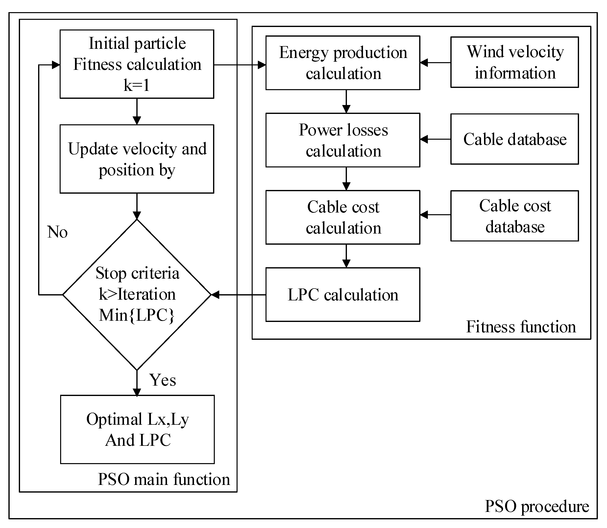
The main factors for the relative placement of WTs in onshore wind farms are the topography and the wake effect between them. The difference in topography and the combination of wake effects affect the other WTs and evaluation of the wake effect considering topography contains a series nonlinear equations and constraints. Besides, the heuristic optimization algorithm is a good choice for the solution of this time-consuming non-convex issue. Therefore, the PSO algorithm is chosen in this paper. The theory is introduced and the optimization procedure is given in the following.

4.1. PSO

Particle Swarm optimization (PSO), which has good performance for solving nonlinear and non-convex problems was proposed by Eberhart and Kennedy in 1995 [29]. Its basic concept comes from the study of foraging behavior of flocks. The feasible solution of each optimization problem can be imagined as a point in the PSO search space, called a particle, and all particles have a fitness value that is determined by the objective function. Each particle has a velocity to determine the direction and the distance it will fly. Velocity and position of each particle will be updated according to their fitness function until the maximum number of iterations is reached. After several iterations, a final stable value should be found, which is called the global optimal solution. The PSO can be modified if needed for different computer configurations and computing needs. Then, the updating velocity v_i and position x_i for particles can be updated as [30]:

$$v_{i+1}=w{v}_i+c_{1}rand\left(p_i-x_i\right)+c_{2}rand\left(g_i-x_i\right)$$

(32)

$$x_{i+1}=x_i+v_i$$

(33)

where w is the coefficient of maintaining the original velocity. If w is larger, the algorithm has a stronger global searching ability while a smaller one improves the local searching ability [31]. c₁ and c₂ are the weight coefficient, normally set to 2. p_i and g_i is the local optimal solution and the global optimal solution, respectively. Rand is random number in the (0,1) interval.

4.2. Onshore Wind Farm Placement Optimization

The distance between adjacent WTs of the entire WF is set to be non-uniform. The simulation procedure to optimize the placement of onshore wind farms by PSO is shown in Figure 7. First, the population is initialized randomly and fitness value of each individual in the population is calculated according to the objective function. Then, a new particle position replaces the previous one and the position will be updated to find the next fitness value repeatedly until the maximum iterations are reached. At that point, L_x and L_y from the optimal outcome will be presented.

5. Results and Discussion

The simulation is implemented on the Matlab R2014a platform (The MathWorks, Inc, Natick, MA, USA). Two test simulations are adopted to verify the feasibility of the proposed model and to find the optimized placement of the onshore wind farm with different topography using the PSO algorithm.

5.1. Case I: Optimized Placement on a Slope

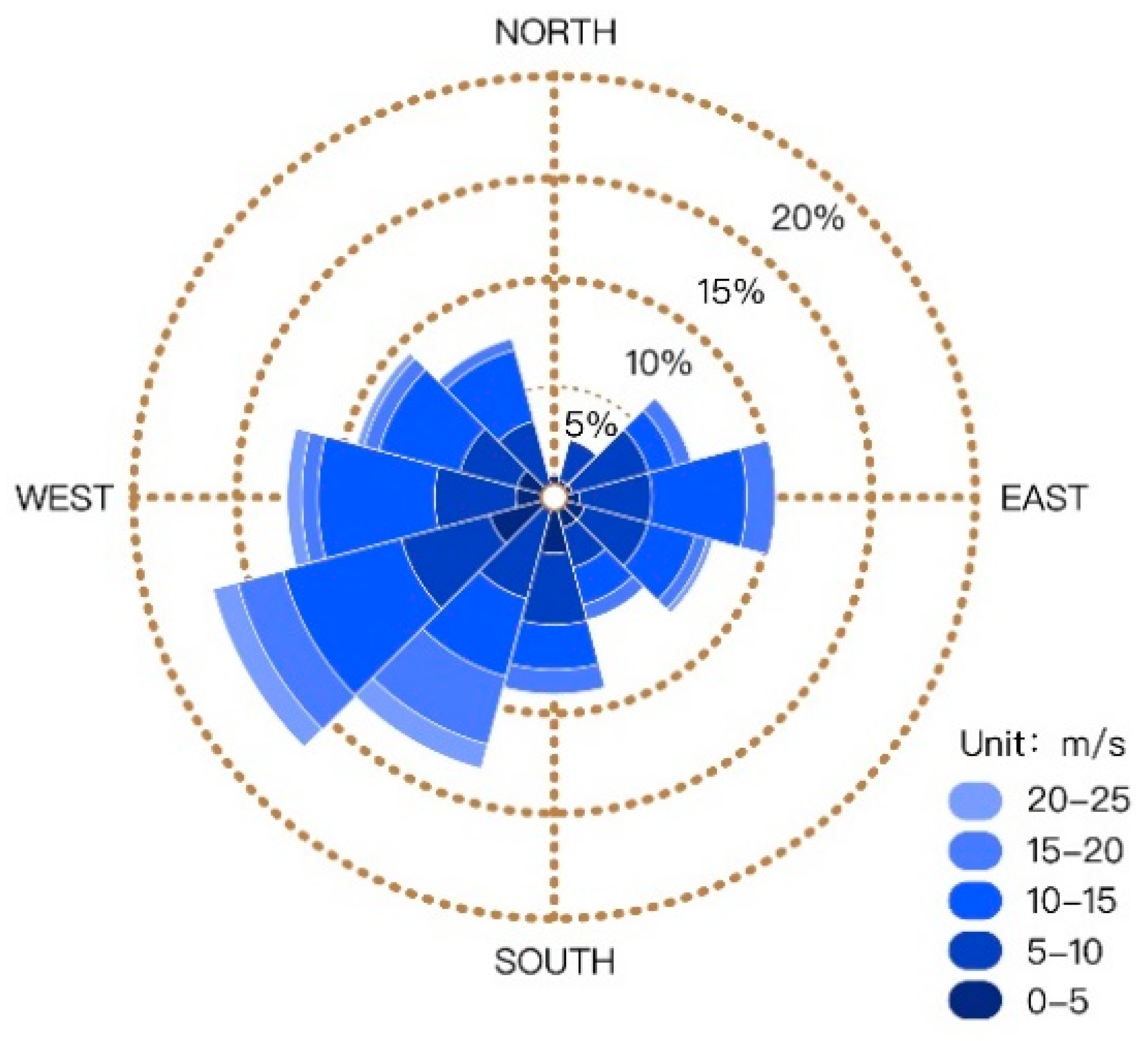
The reference wind farm with 800 MW installed capacity is assumed in the study case [32,33]. In the first simulation case, the wind farm is assumed to be with 10 rows and 8 columns as shown in Figure 5. The WTs (DTU 10 MW WT) are chosen as the reference WTs for an example. In fact, switching to other reference WTs gives the same way for optimization. The parameters of the 10 MW WT are listed in

Table 2. Parameters of 10 MW WT.

Parameter	10 MW DTU WT
Rated wind velocity	11.4 m/s
Cut-in wind velocity	4 m/s
Cut-out wind velocity	25 m/s
Rotor radius	89 m
Hub height	119 m
Rated power	10 MW

[34]. It is worthy noted that the input data of wind speed and wind direction for all cases are obtained from the Norwegian Meteorological Institute and the wind condition is formulated into a wind rose for illustration in Figure 8 [35]. The optimization can be carried out according to different wind conditions considering wind speed and its wind direction. Other factors such as the law are ignored.

As shown in Figure 5, the onshore wind farm is assumed to be sited on a steadily rising slope of 2° in this case. The number indicates that there is a WT in the location of the figure, and the value of one number indicates the total height of the WT. The distance between WTs will be used as the parameters to be optimized.

Information about cables such as conducting sectional areas, voltage levels and so on are obtained from [36]. The 500 and 630 mm² XLPE-Cu HVAV cables with 66 kV rated voltage are chosen for the collection system and the commonly used 1000 mm² Cu HVDC cable with 300 kV rated voltage [37] is chosen for the transmission system as reference standards, respectively.

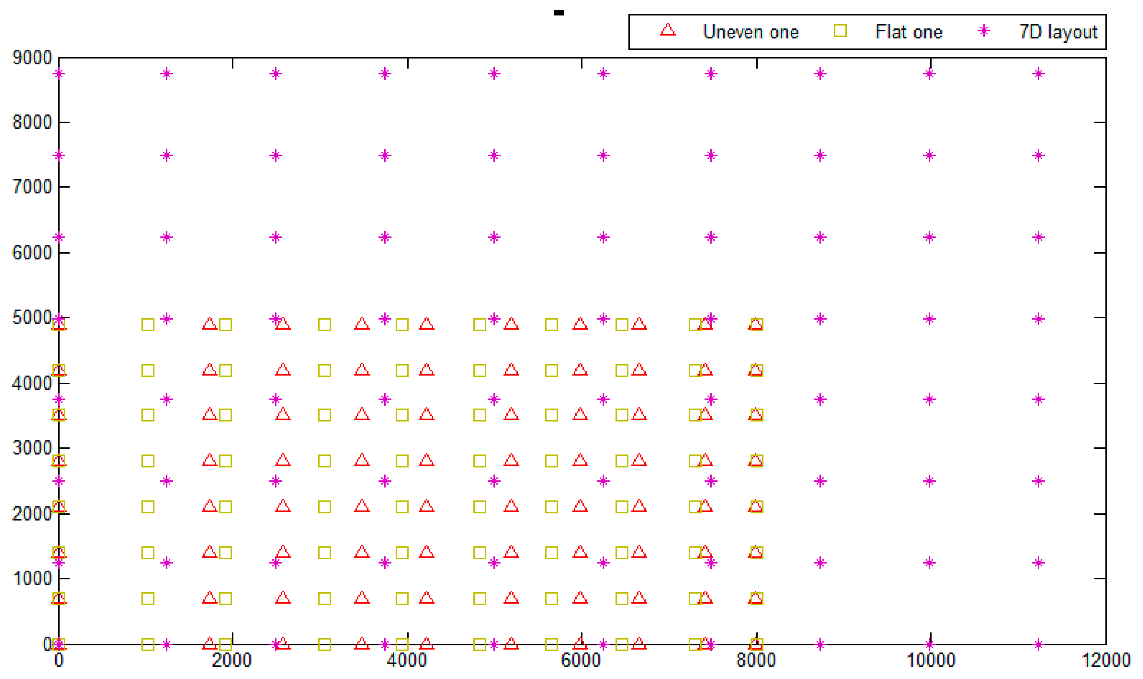
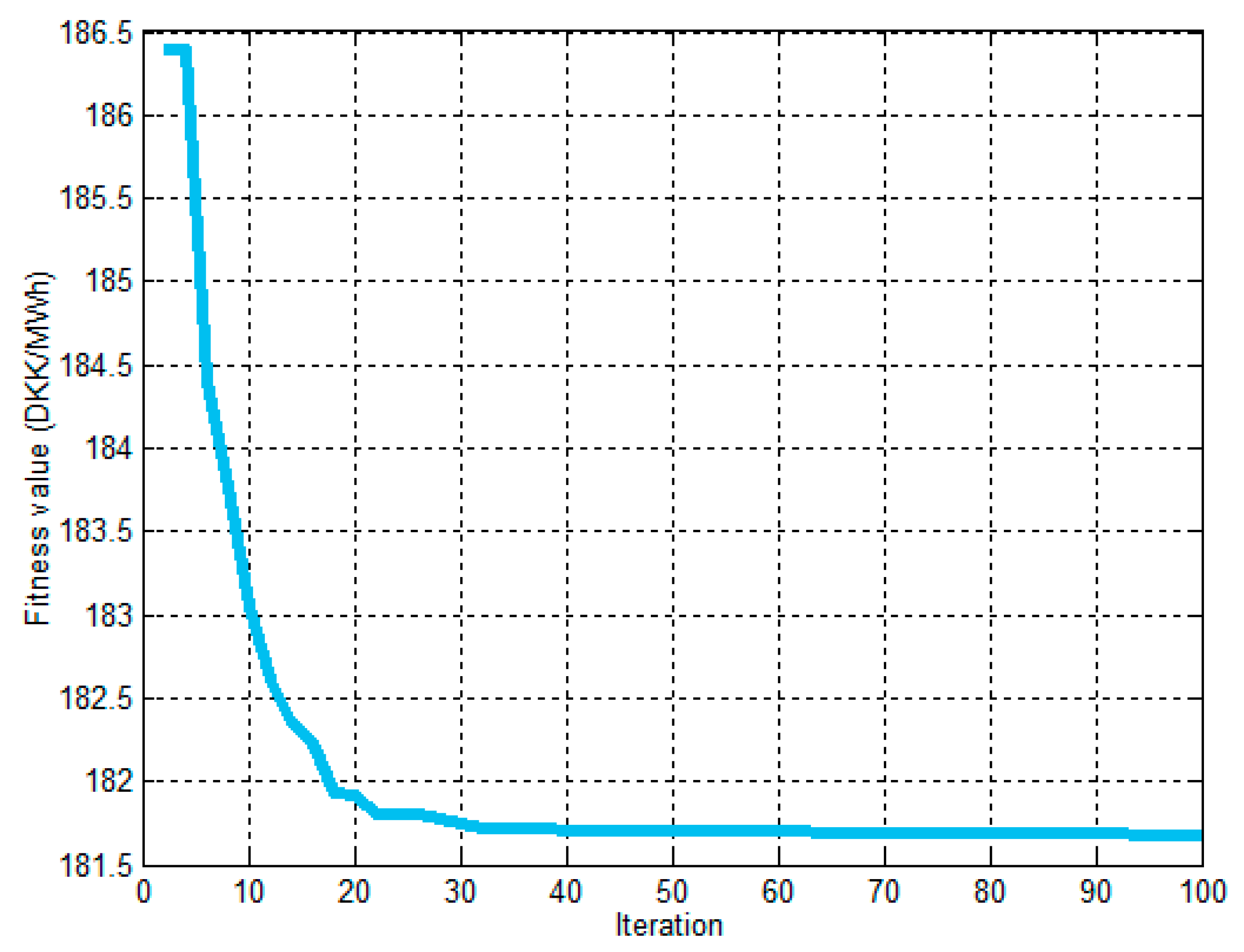
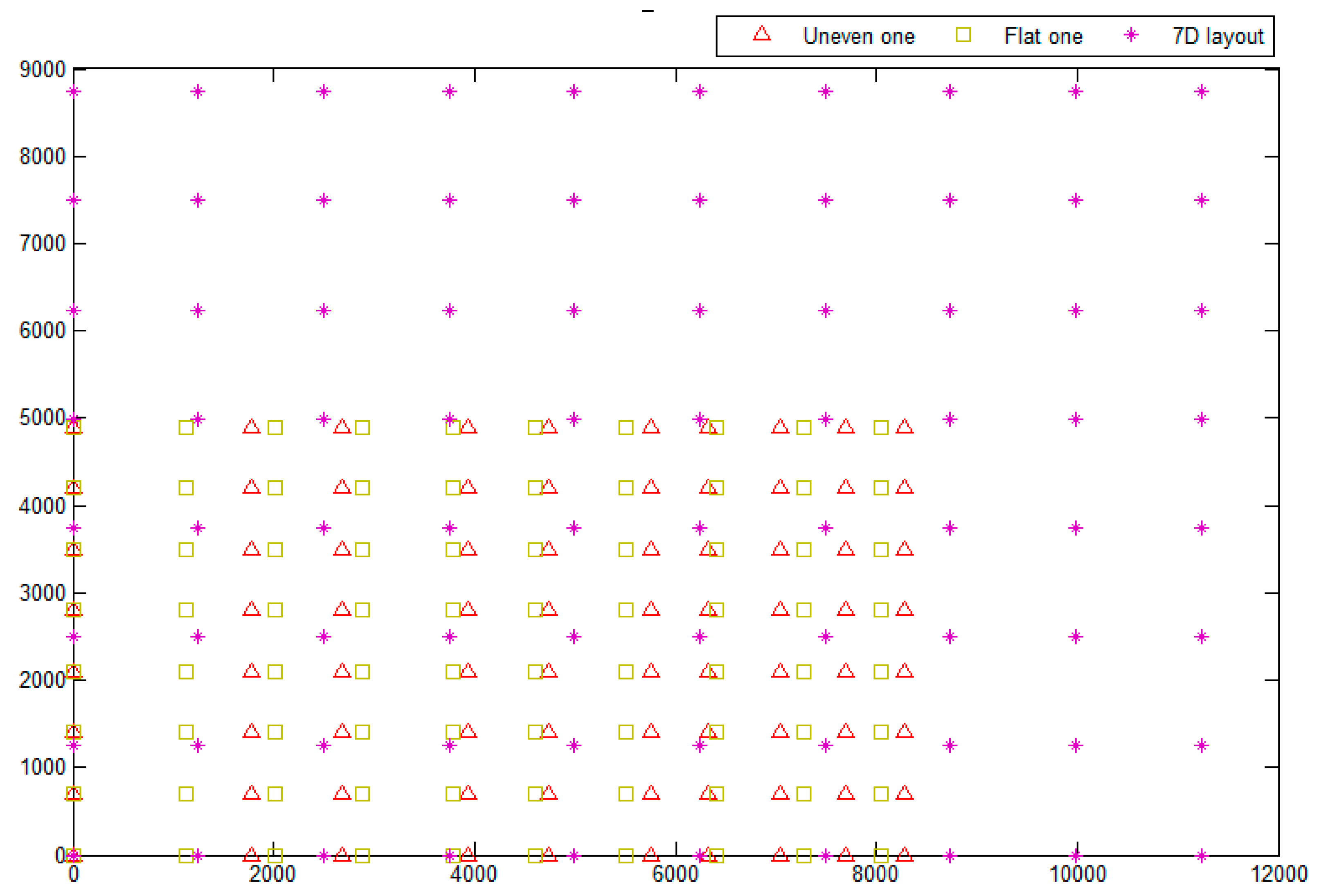
According to the flowchart for optimization using the PSO algorithm, the resulting wind energy production, the costs of cables and the optimization results are presented in

Table 3. Comparison between optimized result of flat ground and slope.

Name	7D Layout	Optimized Layout on Flat Ground	Optimized Sparse Layout on Uneven Flat
Lx (m)	1248	1029.22	1743.15
		895.85	834.51
		1131.78	908.81
		883.22	739.31
		898.93	971.44
		814.68	789.48
		800.33	679.43
		838.50	756.43
		714.39	576.63
Ly (m)	1248	700.21	700.02
Annual energy production (GWh)	4577.55	4164.30	4629.65
Annual energy production without considering wake effect (GWh)	4865.51	4559.28	4978.95
Percentage of wake losses (%)	5.92%	8.67%	7.01%
Cable cost (MDKK)	935.60	843.31	841.11
LPC (DKK/MWh)	204.39	202.51	181.68

. The layout comparison is shown in Figure 9. The fitness value changing with the iteration are shown in Figure 10. The optimized results are compared with the optimized results on the flat ground while the other conditions are exactly the same, so that the difference of the optimized variables, results and the influence of topographical heights can be obtained and compared if the topographical factors are not considered. Also, the standard 7D (diameter) interval layout is compared.

According to the Table 3, no matter what kind of case is chosen, the losses caused by the wake effect reach a non-negligible proportion which were about 8.67% and 7.01% of the total energy production. The smaller percentage of wake loss in the 7D standard layout was due to the overall layout being sloppier than the latter two. It can also be seen in Figure 9 that the occupied area of optimized one on uneven condition is smaller than the other ones. In terms of power production considering wake effect, the optimization results on the slope increased by 11.17% compared with the optimized result on the flat ground and also larger than the standard one. There are two main reasons for this increase: one is that the overall height increased due to the wind shear effect, and the other is that the wake area between the different WTs was relatively reduced due to the height difference. Besides, the LPC was reduced by 11.11% and 10.29% compared with the standard one and the optimized one on flat ground. It is worth noting that the LPC optimized results only represent the same cost model with the optimized results on the ground. For an onshore wind farm that is actually on a non-flat ground, if the layout optimization is performed according to the situation of the flat ground as usual, this will produce an error that cannot be ignored according to Table 3. And the onshore wind farms are often not designed to be flat or actually have a slope but are considered flat due to economic or policy factors. So, it is absolutely necessary to consider the layout optimization for the topographical changes. If the onshore wind farm is designed in a certain slope area after such layout optimization, it can be completely considered because it does not show obvious disadvantages from the perspective of power production. Further, the influence of the terrain also contains other factors such as pressure gradient, more accurate and more complex wake model can be chosen for evaluation [28]. This paper is the first one to explore the concept of this work and more complicated models are not being used since the Jenson model is simple to calculate [7].

5.2. Case II: Optimized Placement on a Hill

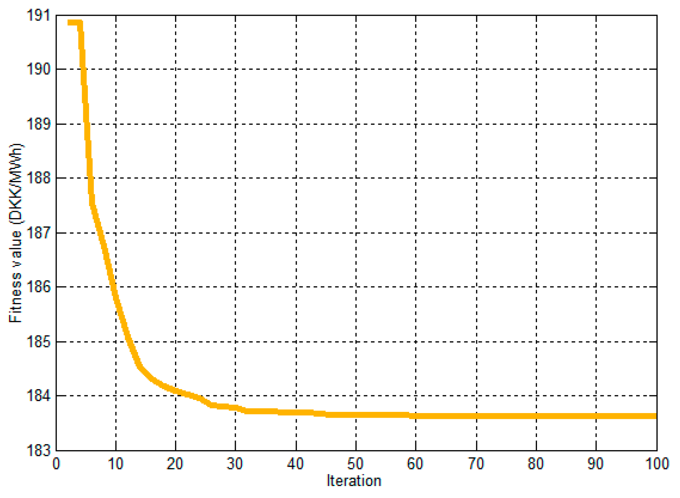
In this case study, the reference layout was assumed to be located on a small hill where the slope first rises and then drops as shown in Figure 11. Both the uphill and downhill slope angles α were 2 degrees. The fitness value changing with iteration are shown in Figure 12, and the case results were compared with the standard one and also the optimized layout on the flat ground to illustrate the need for this consideration and the difference in layout in

Table 4. Comparison between optimized results of flat ground and hill.

Name	7D Layout	Optimized Layout on Flat Ground	Optimized Sparse Layout on Uneven Flat
Lx (m)	1248	1131.28	1786.55
		881.18	901.16
		874.11	1249.45
		900.14	807.68
		822.39	1019.60
		896.53	554.73
		901.37	728.13
		866.05	642.26
		769.07	587.63
Ly (m)	1248	700.35	700.01
Annual energy production (GWh)	4577.55	4125.94	4603.05
Annual energy production without considering wake effect (GWh)	4865.51	4559.28	4954.02
Percentage of wake losses (%)	5.92%	9.50%	7.08%
Cable cost (MDKK)	935.60	836.37	845.26
LPC (DKK/MWh)	204.39	202.71	183.63

. Also, the layouts are given in Figure 13.

Compared with Case I, the power production of Case II decreased because the wind farm is assumed on a hill where almost half the number of WTs is at a lower terrain, which makes the wind velocity lower due to the shear effect. Similarly, the change in topographical height cannot be ignored in layout optimization problems. If the terrain is not considered for the onshore wind farm, the optimized results may be subject to certain errors. Regarding the two optimization results, the power production of the optimization results on the hill is increased by 11.56% compared with the optimized layout of flat ground while the LPC is reduced by 9.41%. A similar layout compared with Case I is because the reference wind farm is similar, although the terrain changes, but the overall layout framework is the same. Therefore, the change of the WTs spacing was mainly to reduce the mutual wake effect among WTs. In fact, slight changes in spacing can significantly change the energy losses between them due to wake effect, thereby changing the total power production and the cost. Some explanations for the energy production comparison are the same as in Case I.

6. Conclusions and Future Work

The paper focuses on the optimized placement of wind turbines for three-dimensional onshore wind farms. The optimized layout of WTs in onshore wind farms was proposed by focusing on variations in topography and the effect of this on wind turbine interactions. Two cases, namely, where the onshore wind farm was on a slope and on a small hill where the slope first rises then drops are considered. The simulation results show the main influencing factors: the topography and the wake effect for the relative placement of WTs cannot be ignored in optimization process. The proposed optimized placement of WTs in onshore wind farms improved the LPC by 3.40% and 2.25%, respectively, in the two study cases. This proves the feasibility and applicability of the proposed optimized placement method. The proposed method can be extended to other topographic conditions for onshore wind farms.

Future research work may take the following approach: It would be interesting to extend the scope of this scenario with considering active wake monitoring by yawing the turbines actively out of the wake during operational years. The wind farm layout optimization and turbine operational optimization can be connected. Perhaps the next step of future work can be started from it.

References

- GWEC Report 2018. Available online: https://gwec.net/global-wind-report-2018/ (accessed on 21 June 2019).
- Ma, Y.; Yang, H.; Zhou, X.; Li, J.; Wen, H. The dynamic modeling of wind farms considering wake effects and its optimal distribution. In Proceedings of the 2009 World Non-Grid-Connected Wind Power and Energy Conference, Nanjing, China, 24–26 September 2009. [Google Scholar]
- Barthelmie, R.J.; Larsen, G.C.; Frandsen, S.T.; Folkerts, L.; Rados, K.; Pryor, S.C.; Lange, B.; Schepers, G. Comparison of wake model simulations with offshore wind turbine wake profiles measured by sodar. J. Atmos. Oceanic Technol. 2006, 23, 888–901. [Google Scholar] [CrossRef]
- Wang, P.; Goel, L.; Ding, Y.; Chang, L.P.; Andrew, M. Reliability-based long term hydro/thermal reserve allocation of power systems with high wind power penetration. In Proceedings of the 2009 IEEE Power & Energy Society General Meeting, Calgary, AB, Canada, 26–30 July 2009. [Google Scholar]
- Ela, E.; Kirby, B.; Lannoye, E.; Milligan, M.; Flynn, D.; Zavadil, B.; O’Malley, M. Evolution of operating reserve determination in wind power integration studies. In Proceedings of the IEEE PES general meeting, Providence, RI, USA, 25–29 July 2010. [Google Scholar]
- WindPRO/PARK. Introduction Wind Turbine Wake Modelling and Wake Generated Turbulence; EMD International A/S: Aalborg, Denmark, 2006. [Google Scholar]
- Jensen, N.O. A Note on Wind Generator Interaction, RISØ-M-2411; Risø National Laboratory: Roskilde, Denmark, 1983. [Google Scholar]
- Ainslie, J.F. Calculating the flowfield in the wake of wind turbines. J. Wind Eng. Ind. Aerodyn. 1988, 27, 213–224. [Google Scholar] [CrossRef]
- Larsen, G.C.; Højstrup, J.; Madsen, H.A. Wind fields in wakes. In Proceedings of the European Union Wind Energy Conference (EUWEC’96), Göteborg, Sweden, 20–24 May 1996; pp. 764–768. [Google Scholar]
- Westerhellweg, A.; Neumann, T. CFD simulations of wake effectsa at the alpha ventus offshore wind farm. In Proceedings of the EWEA, Brussels, Belgium, 14–17 March 2011. [Google Scholar]
- Mosetti, G.P.C.D.B.; Poloni, C.; Diviacco, B. Optimization of wind turbine positioning in large wind farms by means of a genetic algorithm. J. Wind Eng. Ind. Aerodyn. 1994, 51, 105–116. [Google Scholar] [CrossRef]
- Grady, S.A.; Hussaini, M.Y.; Abdullah, M.M. Placement of wind turbines using genetic algorithms. Renewable Energy 2005, 30, 259–270. [Google Scholar] [CrossRef]
- Marmidis, G.; Lazarou, S.; Pyrgioti, E. Optimal placement of wind turbines in a wind park using Monte Carlo simulation. Renewable Energy 2008, 33, 1455–1460. [Google Scholar] [CrossRef]
- Rahbari, O.; Vafaeipour, M.; Fazelpour, F.; Feidt, M.; Rosen, M.A. Towards realistic designs of wind farm layouts: Application of a novel placement selector approach. Energy Convers. Manage. 2014, 81, 242–254. [Google Scholar] [CrossRef]
- Hou, P.; Hu, W.; Soltani, M.; Chen, Z. Optimized placement of wind turbines in large-scale offshore wind farm using particle swarm optimization algorithm. IEEE Trans. Sustainable Energy 2015, 6, 1272–1282. [Google Scholar] [CrossRef]
- Hou, P.; Hu, W.; Chen, C.; Soltani, M.; Chen, Z. Optimization of offshore wind farm layout in restricted zones. Energy 2016, 113, 487–496. [Google Scholar] [CrossRef]
- Wang, L.; Tan, A.C.C.; Cholette, M. Comparison of the effectiveness of analytical wake models for wind farm with constant and variable hub heights. Energy Convers. Manage. 2016, 124, 189–202. [Google Scholar] [CrossRef] [Green Version]
- Vasel-Be-Hagh, A.; Archer, C.L. Wind farm hub height optimization. Appl. Energy 2017, 195, 905–921. [Google Scholar] [CrossRef]
- Palma, J.M.L.M.; Castro, F.A.; Ribeiro, L.F.; Rodrigues, A.H.; Pinto, A.P. Linear and nonlinear models in wind resource assessment and wind turbine micro-siting in complex terrain. J. Wind Eng. Ind. Aerodyn. 2008, 96, 2308–2326. [Google Scholar] [CrossRef]
- Song, M.X.; Chen, K.; He, Z.Y.; Zhang, X. Optimization of wind farm micro-siting for complex terrain using greedy algorithm. Energy 2014, 67, 454–459. [Google Scholar] [CrossRef]
- González-Longatt, F.; Wall, P.; Terzija, V. Wake effect in wind farm performance: Steady-state and dynamic behavior. Renewable Energy 2012, 39, 329–338. [Google Scholar] [CrossRef]
- Mathew, S. Fundamentals, Resource Analysis and Economics. In Wind Energy, 1st ed.; Springer: New York, NY, USA, 2006. [Google Scholar]
- Qiao, W. Intelligent mechanical sensorless MPPT control for wind energy systems. In Proceedings of the 2012 IEEE Power and Energy Society General Meeting, San Diego, CA, USA, 22–26 July 2012; pp. 1–8. [Google Scholar]
- Gonzalez, J.S.; Payan, M.B.; Santos, J.R. Optimum Wind Turbines Operation for Minimizing Wake Effect Losses in Offshore Wind Farms. In Proceedings of the 13th International Conference on Environment and Electrical Engineering (EEEIC), Wroclaw, Poland, 1–3 November 2010; pp. 188–192. [Google Scholar]
- Flores, P.; Tapia, A.; Tapia, G. Application of a control algorithm for wind speed prediction and active power generation. Renewable Energy 2005, 30, 523–536. [Google Scholar] [CrossRef]
- Lundberg, S. Performance Comparison of Wind Park Configurations; Technical Report No. 30R; Department of Electric Power Engineering, Chalmers University of Technology: Goteborg, Sweden, 2003. [Google Scholar]
- Zhao, M. Optimization of Electrical System for Offshore Wind Farms via a Genetic Algorithm Approach. Ph.D. Thesis, Institute of Energy Technology, Aalborg University, Aalborg, Denmark, 2006. [Google Scholar]
- Shamsoddin, S.; Porté-Agel, F. Wind turbine wakes over hills. J. Fluid Mech. 2018, 855, 671–702. [Google Scholar] [CrossRef]
- Kennedy, J. Particle Swarm Optimization. In Proceedings of the International Conference on Neural Networks, Perth, Australia, 27 November–1 December 2011. [Google Scholar]
- Kennedy, J. The particle swarm: Social adaptation of knowledge. In Proceedings of the 1997 IEEE International Conference on Evolutionary Computation (ICEC ’97), Indianapolis, IN, USA, 13–16 April 1997; pp. 303–308. [Google Scholar]
- Hu, M.; Wu, T.; Weir, J.D. An adaptive particle swarm optimization with multiple adaptive methods. IEEE Trans. Evol. Comput. 2012, 17, 705–720. [Google Scholar] [CrossRef]
- R&D centre Kiel University of Applied Sciences GmbH, FINO3-Research Platform in the North Sea and the Baltic No. 3. Available online: http://www.fino3.de/en/ (accessed on 04 June 2019).
- Norwegian Centre for Offshore Wind Energy (NORCOWE). (2014, Sep. 9). WP2014-Froysa-NRWF NORCOWE Reference Wind Farm. Available online: http://www.norcowe.no/ (accessed on 05 June 2019).
- Bak, C.; Zahle, F.; Bitsche, R.; Kim, T.; Yde, A.; Henriksen, L.C.; Hansen, M.H.; Blasques, J.P.A.A.; Gaunaa, M.; Natarajan, A. The DTU 10-MW Reference Wind Turbine. 2013. Available online: https://orbit.dtu.dk/files/55645274/The_DTU_10MW_Reference_Turbine_Christian_Bak.pdf (accessed on 05 June 2019).
- The Norwegian Meteorological Institute. Available online: http://met.no/English/ (accessed on 15 June 2019).
- ABB, XLPE. Submarine Cable Systems Attachment to XLPE Land Cable Systems—User’s Guide; ABB Corporation: Fredericia, Denmark, 2013. [Google Scholar]
- Cables, ABB High Voltage. HVDC Light Cables—Submarine and Land Power Cables; ABB Corporation: Fredericia, Denmark, 2013. [Google Scholar]
Figure 1.
Wake effect between wind turbines (WTs) on a slope.
Figure 2.
Wake model considering topographical difference. (a) Downstream WT is higher. (b) Downstream WT is lower.
Figure 3.
Overlapped wake area analysis. (a) WTs in the same topographic height presented in three-dimensional coordinates z-x-y. (b) WTs in the different topographic heights presented in vertical coordinate z-x.
Figure 4.
Three conditions in wake effect.
Figure 5.
Matrix storage for topography definition.
Figure 6.
Framework for calculating the power production.
Figure 7.
Flowchart for wind farm layout optimization using particle swarm optimization (PSO) algorithm.
Figure 8.
Wind condition for cases.
Figure 9.
Layout comparison of Case I.
Figure 10.
Fitness values of Case I change with iterations.
Figure 11.
Case II wind farm placement.
Figure 12.
Fitness values of Case II change with iterations.
Figure 13.
Layout comparison of Case II.