Structural Analysis of Large-Scale Vertical-Axis Wind Turbines, Part I: Wind Load Simulation


1
Department of Civil and Environmental Engineering, The Hong Kong Polytechnic University, Hong Kong, China
2
China Energy Engineering Group Guangdong Electric Power Design Institute Co. Ltd., Guangzhou 510663, China
3
College of Civil Engineering and Mechanics, Huazhong University of Science and Technology, Wuhan 430074, China
4
Shenzhen Graduate School, Harbin Institute of Technology, Shenzhen 518055, China
*
Author to whom correspondence should be addressed.
Energies 2019, 12(13), 2573; https://doi.org/10.3390/en12132573
Submission received: 10 February 2019
/
Revised: 28 May 2019
/
Accepted: 30 May 2019
/
Published: 4 July 2019
(This article belongs to the Section A3: Wind, Wave and Tidal Energy)
Abstract
:When compared with horizontal-axis wind turbines, vertical-axis wind turbines (VAWTs) have the primary advantages of insensitivity to wind direction and turbulent wind, simple structural configuration, less fatigue loading, and easy maintenance. In recent years, large-scale VAWTs have attracted considerable attention. Wind loads on a VAWT must be determined prior to structural analyses. However, traditional blade element momentum theory cannot consider the effects of turbulence and other structural components. Moreover, a large VAWT cannot simply be regarded as a planar structure, and 3D computational fluid dynamics (CFD) simulation is computationally prohibitive. In this regard, a practical wind load simulation method for VAWTs based on the strip analysis method and 2D shear stress transport (SST) k-ω model is proposed. A comparison shows that the wind pressure and aerodynamic forces simulated by the 2D SST k-ω model match well with those obtained by 2.5D large eddy simulation (LES). The influences of mean wind speed profile, turbulence, and interaction of all structural components are considered. A large straight-bladed VAWT is taken as a case study. Wind loads obtained in this study will be applied to the fatigue and ultimate strength analyses of the VAWT in the companion paper.
1. Introduction
Renewable energy, especially wind energy, increasingly attracts the interest of the world nowadays. Vertical-axis wind turbines (VAWTs) are currently being developed to take advantage of wind power. Wind loads on a VAWT at the aerodynamic force and wind pressure levels must be comprehensively investigated. The aerodynamic forces, especially the tangential forces on the blades of the VAWT, must be estimated accurately to assess the power production of a VAWT. On the other hand, wind pressures are required to calculate the local stresses/strains of the components, especially the blades, for the fatigue and ultimate strength analyses.
Several tools to estimate wind loads of VAWTs have been proposed, such as double multiple stream-tube theory (DMST), vortex model, and computational fluid dynamics (CFD) simulation [1]. DMST is the simplest and most widely used method. However, this method cannot consider the influence of the arms and tower on wind loads acting on the blades. The method can only obtain aerodynamic forces, but not wind pressures on the blades. Although the vortex model can consider the influences of other structural components and obtain wind pressures, the computational cost is higher than that of DMST, and the accuracy of this method is lower than that of CFD. Many researchers now simplify a VAWT as a planar structure and conduct 2D or 2.5D CFD simulation to analyze the aerodynamic forces on VAWTs. Researchers have put a lot of effort into the important issues, such as CFD settings [2,3,4,5], turbulence model comparison [6,7], 2.5D simulation [8], airfoil profile [9], blade–vortex interaction [10], unsteady performance [11,12,13,14], and dynamic stall [15,16,17,18]. Nevertheless, the wind speed along the height of a VAWT is not uniform, which does not match 2D or 2.5D simulation. Furthermore, the computational cost of CFD turbulence modeling for a 3D VAWT is high [19,20,21,22]. Some references concern the influence of the fluid–structure interaction [23,24,25]. These studies help to reveal the in situ aerodynamics and dynamic responses of VAWTs, while the complexity of the simulation and the intensive time consumption prevent applications in the industry community. As a result, an efficient simulation method is required to estimate the wind loads on the VAWT to consider the influence of all structural components on the wind field of a VAWT and the varying wind speed along the height of the VAWT.
Nearly all researchers adopt the steady inflow boundary and ignore the turbulent inflow, while turbulence is important and may lead to performance loss [26]. For horizontal-axis wind turbines (HAWTs), the influence of turbulent inflow has been studied for years [27]. A basic method is to use blade element momentum theory and Taylor’s frozen hypothesis to calculate the aerodynamic forces. Empirical dynamic inflow models have also been proposed [28]. However, these methods are used for HAWTs only. The aerodynamics of a VAWT is different from that of a HAWT. Studies to verify the applicability of these methods for VAWTs are also insufficient. As a result, the performance of a VAWT in unsteady wind conditions has attracted considerable attention in recent years [14,29,30,31,32,33]. However, only simple sinusoidal variation wind speeds are considered in these studies, which is different from the real atmospheric turbulent inflow. Therefore, the turbulent inflow on wind loads must be further explored.
In this paper, a simulation method of determining wind loads, including wind pressures and aerodynamic forces, on the entire VAWT is proposed. The details are provided in Section 2. A straight-bladed VAWT built in Yangjiang City, Guangdong Province, China is taken as an example to demonstrate the proposed method. Two-dimensional (2D) shear stress transport (SST) k-ω simulation is used to compute wind loads on the VAWT, and the results are compared with those of 2.5D large eddy simulation (LES) in Section 3. The framework based on the strip analysis method and 2D CFD simulation is then applied to the straight-bladed VAWT to determine its wind loads in Section 4. The influences of the existence of arms and tower on the aerodynamic forces and wind pressures on the blades, the variation in mean wind speed along the height of the VAWT, and the effects of the turbulent wind are all considered and discussed in Section 4. The concluding remarks are provided in Section 5.
2. Wind Load Simulation Framework for VAWTs
2.1. Straight-Bladed VAWT
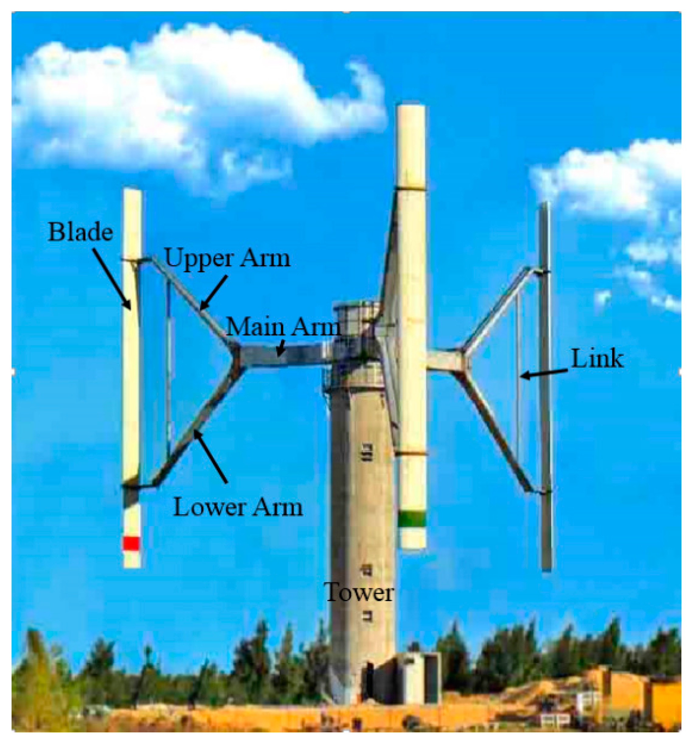
The wind load simulation framework proposed here is generally applicable to any type of VAWTs. Figure 1 shows a large-scale lift-type straight-bladed VAWT, which is taken as an example to illustrate the framework, without losing generality.
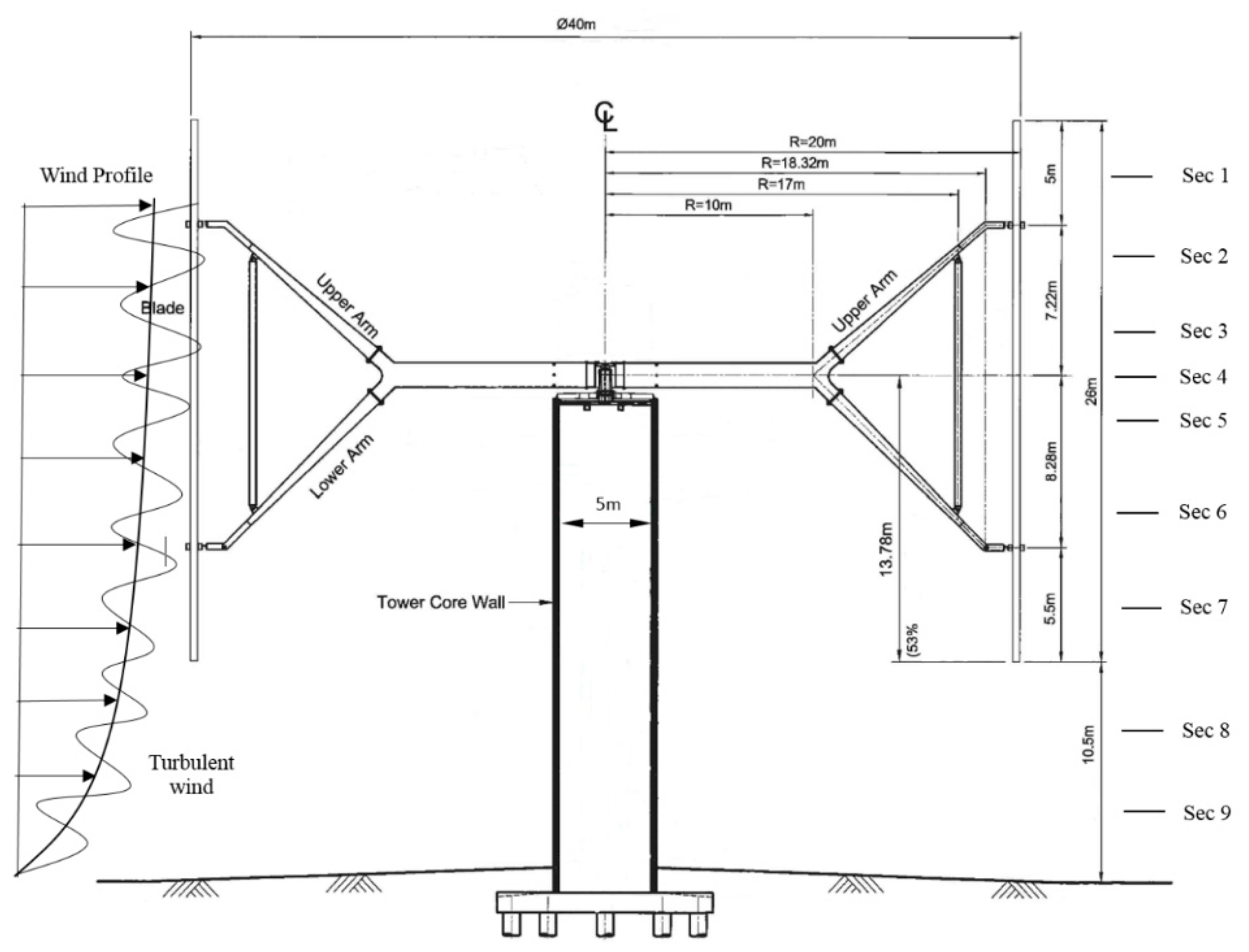
The prototype VAWT was constructed at Yangjiang City of Guangdong Province, China by Hopewell Holdings Limited of Hong Kong. The tower of the VAWT is made of reinforced concrete with a height of 24 m and a diameter of 5 m (Figure 2). The thickness of reinforced concrete wall of the tower is 250 mm. The tower supports a vertical rotor with the rotating parts of the VAWT of a height of 26 m and a diameter of 40 m. Three blades of the rotor are equally arranged at an interval angle of 120°. The blades are of NACA0018 type with a chord length of 2 m and a vertical height of 26 m. Each blade is made of glass fiber-reinforced plastic laminate materials and is supported by a Y-type steel arm connecting to the tower via the main shaft at the top of the tower (the hub height). The ground clearance of the bottom end of the blades is 10.5 m. Each Y-type steel arm consists of a main arm, an upper arm, and a lower arm, as shown in Figure 2. The cross section of the main arm is rectangular with a width of 1.6 m, a height of 1.2 m, and a length of 10 m. The upper and lower arms support the blade at one end and are connected to the main arm at another end. The cross section of the upper and lower arms is rectangular with a constant width of 1.2 m and a varying depth from 0.6 m at the main arm side to 0.3 m at the blade side. A 0.2 m diameter vertical rod links the lower and upper arms.
2.2. Wind Conditions
The mean and turbulent wind speeds should be considered in determining the wind loads on a VAWT during its operation. In the atmospheric boundary layer, the mean wind speed near the ground approaches zero and then increases with the increase in height. Two types of mean wind speed profiles are often used. One is the semi-empirical logarithmic law, and the other is the empirical power law. The power law, which is described in Figure 2, is used in this study because of its simplicity.
where z is the height above the ground; V(z) is the mean wind speed at z; Vhub is the reference mean wind speed at the hub height, zhub; and exponent α is the empirically derived coefficient that depends on the stability of the atmosphere and the surface roughness [34,35]. A value of α = 0.2 is suggested by IEC61400-1 [36]. The power law or a logarithmic wind profile is approximate. Therefore, there is an uncertainty in the mean wind speed at the hub height, and thus the aerodynamic forces and the estimated output power. Some researchers have presented corrections of the model [37], although more studies on this topic are necessary.
Several power spectra and coherence models have been proposed to model the turbulent wind at different heights. In this study, only the longitudinal turbulent wind is considered because the lateral turbulent wind speed is relatively small and the vertical turbulent wind speed will not affect the wind loads on the VAWT. The mean wind speed and the longitudinal turbulent wind are assumed to be uniform across the wind turbine at any given horizontal level. Thus, the turbulent wind speed at each height can be regarded as a 1D stochastic process.
For simulating the longitudinal turbulent wind speed at a given height, the Kaimal spectrum and the corresponding coherence function [27,36] recommended by IEC61400-1 [36] are selected as
where S(f, z), σu, and Lu are the power spectrum, standard deviation, and integral length scale of the longitudinal turbulence at height z, respectively; f is the frequency; Δz is the distance between the two heights (Δz = |z1 − z2|); V(z) is the mean wind speed at the two heights considered, which is equal to [V(z1) + V(z2)]/2; and Lc is the coherence scale parameter. σu, Lu, and Lc can be determined by IEC61400-1 [36]. Equation (3) is an empirical exponential model and is widely adopted by wind turbine design standards, such as IEC61400-1 [36]. Once the power spectrum of the longitudinal turbulence is established, the turbulent wind speed time histories along the height of the VAWT can be generated using the spectral representation method [38].
The extreme wind speed with a 50-year return period should be considered to determine the wind loads on a VAWT under the extreme wind speed condition. In this case, the VAWT is locked and stands still. Similar to the operational wind speed condition, the mean wind profile and the longitudinal turbulent wind speed must be considered. Only the ultimate strength analysis is required in the case, and the fatigue analysis is unnecessary. The widely used equivalent static wind load (ESWL) method is adopted in this study. Different methods for the evaluation of the peak factor in the ESWL method have been proposed [39]. A peak factor of approximately 3.5 and the following steady wind extreme model are suggested by IEC61400-1 [36].
where Ve50 is the extreme wind speed with a recurrence period of 50 years and Vref is the reference wind speed depending on the wind turbine class. Class I is considered in this study, and Vref is thus equal to 50 m/s [36]. The exponent is taken as 0.11 under the extreme wind condition. Thus, the analysis under the extreme wind condition can be regarded as a steady analysis.
2.3. Strip Analysis Method
The above-mentioned discussions show that the mean wind speed and the structural configuration vary along the height, and the turbulent wind speeds at different heights are dissimilar but correlated. Therefore, the wind loads cannot be determined by only simplifying the VAWT as a planar structure. High-fidelity simulations [40] can give more accurate results based on which wind loads and output power can be estimated more precisely, while a 3D CFD simulation of the wind loads on a VAWT is extremely computationally intensive.
The strip analysis method is proposed in this study to take advantage of 2D CFD simulation and consider the varying wind loads on varying cross sections of the VAWT. The strip method is widely used in the analysis of propellers [41] and bridges [42], in which the 3D propeller or the bridge is divided into several sections and the 2D simulation is then conducted on each section. In a similar way, the entire VAWT is divided into several typical cross sections along its height, and the 2D simulation is applied to each section with the simulated mean and turbulent wind speeds.
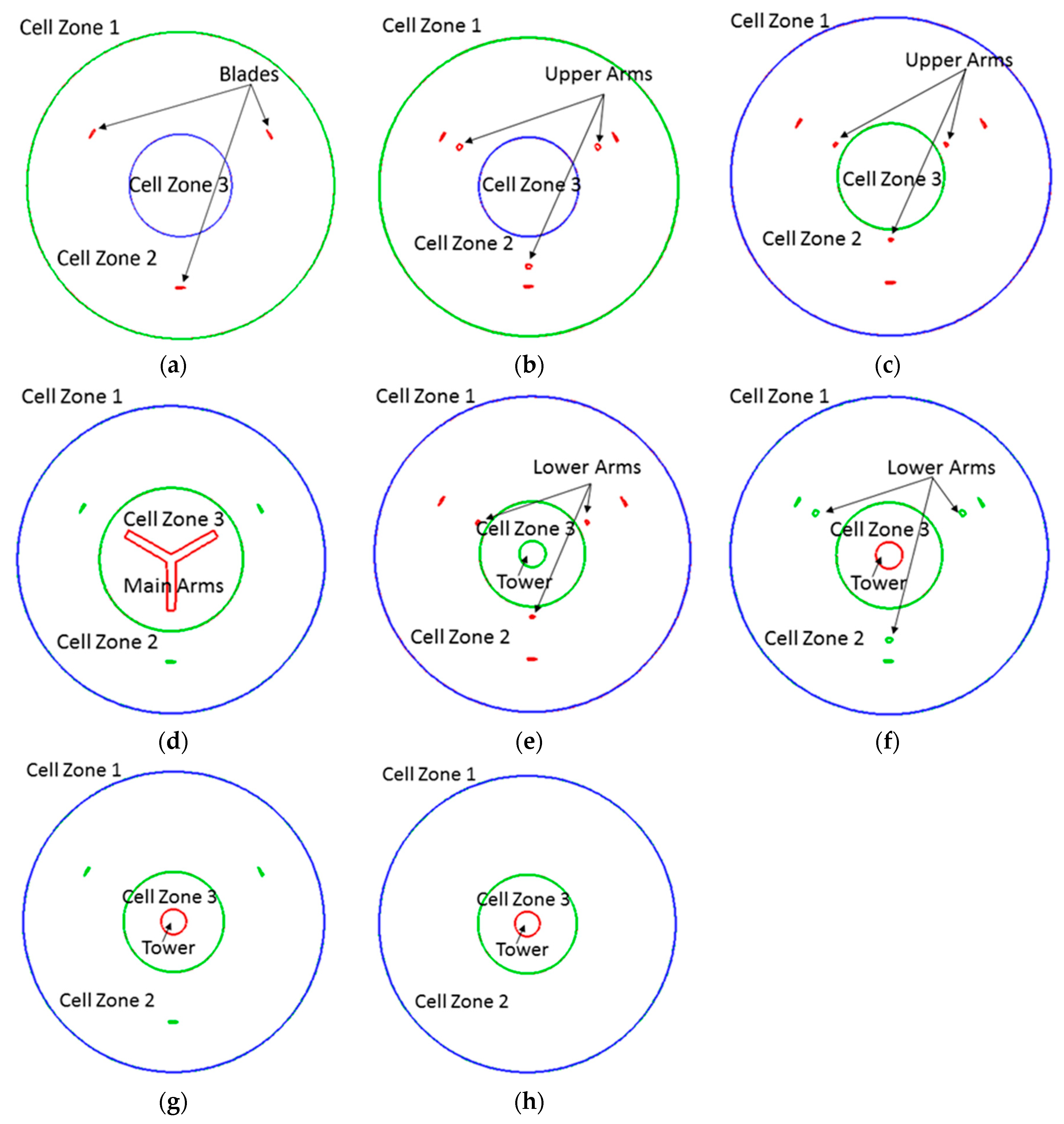
As shown in Figure 2, nine cross sections of the VAWT, namely, Sec 1–Sec 9, are chosen for the analysis on structural configuration and variation in wind speed. Their elevations are listed in Table 1. The plan of the cross sections is shown in Figure 3. For example, Sec 1 has the cross sections of three blades only (Figure 3a), Sec 2 has the blades and the upper arms (Figure 3b), and Sec 8 has the tower only (Figure 3h). Notably, Sec 4 is at the hub height, zhub. Cell zones 1–3 in the figures are introduced in Section 3.1.
After the wind loads of all nine sections are simulated, they are used collectively and synchronously to yield the 3D wind load field on the VAWT.
3. Validity of SST k-ω for Wind Load Simulation
Either 2D or 2.5D CFD simulation can be considered for each cross section. For a VAWT, the SST k-ω and the LES are the two most widely used turbulence models. Li et al. [8] compared different simulation methods and suggested that 2.5D LES predicts better results than the experimental data. However, the computational cost of LES is high. Considering several sections and wind speed cases, the total computation is demanding. Meanwhile, SST-RANS, such as SST k-ω, is superior to standard k-ε in the ability to predict flow separation [43]. The 2D SST k-ω simulation is an excellent option for the VAWT problem concerned in this study owing to its efficiency and precision. In this section, the 2D SST k-ω model and 2.5D LES are used to simulate the wind loads, and the results of the two approaches are compared with each other.
3.1. CFD Simulation Strategy
Three techniques, namely, sliding, dynamic, and overlapping meshes, can be used to simulate the flow field around a rotating VAWT [7,8,19]. The sliding mesh technique is often adopted in the simulation of wind loads on a 2D VAWT because of its wide application range and simplicity [2,8,11,41]. This technique requires the flow field to be discretized into several zones, and the data of these zones can be transformed to one another through sliding interfaces. In this study, the sliding mesh technique is adopted in the 2D SST k-ω simulation and 2.5D LES.
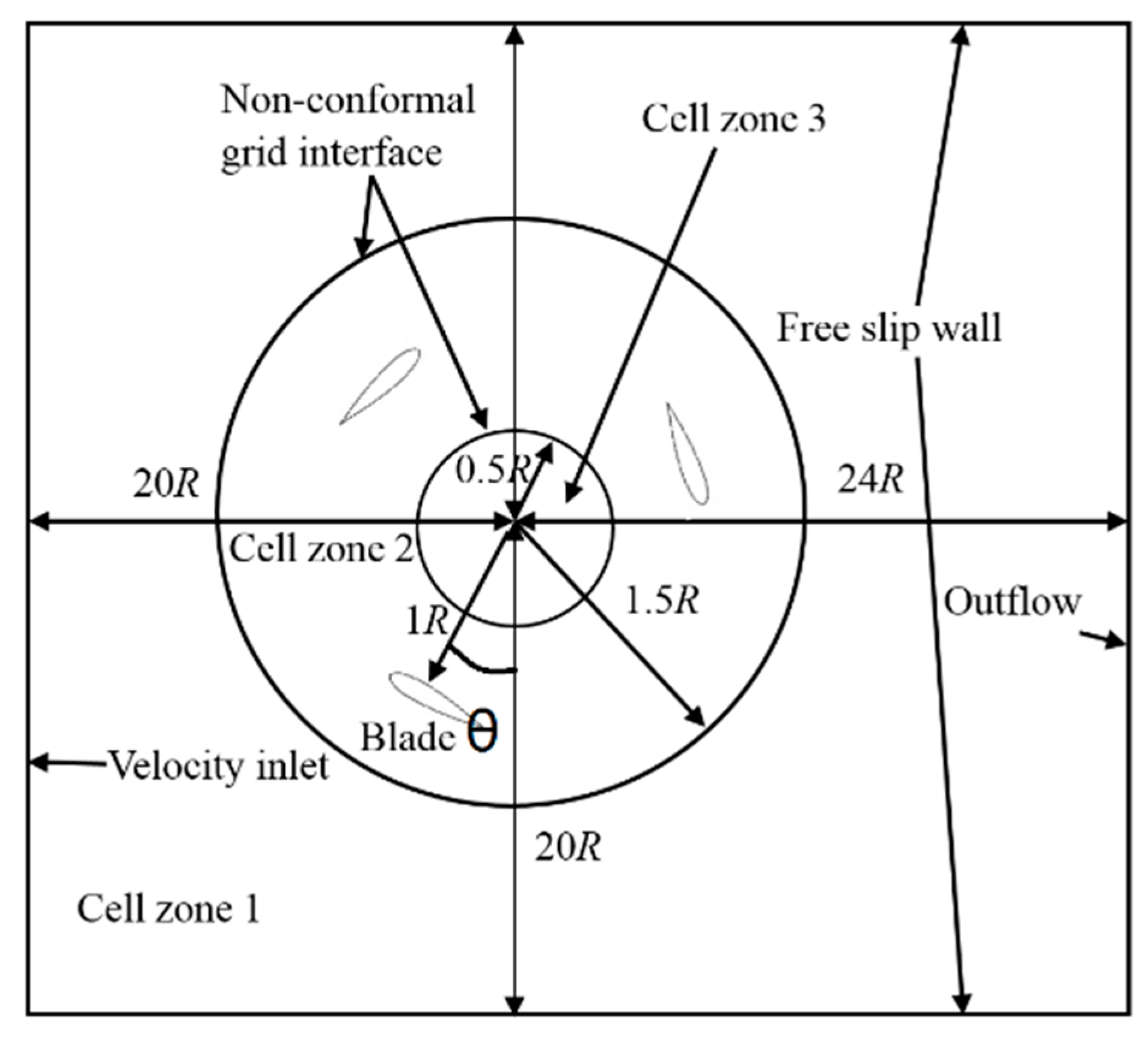
The two methods are compared with Sec 7 as an example, which is a typical section of the VAWT including the tower and blades. The geometry and boundaries of the flow field around the VAWT are shown in Figure 4. The radius of the rotor is R = 20 m. The velocity inlet is located at 400 m (20 R) in front of the VAWT, and the outlet is placed at 480 m (24 R) behind the VAWT to ensure the full development of wake. The side boundaries are 400 m (20 R) away from the center of the rotor to eliminate the blockage effect. A free-slip wall boundary condition is applied, in which the normal velocity components and the normal gradients of all velocity components are assumed to be zero.
The mesh grids are divided into three zones, cell zones 1–3, as shown in Figure 4. The meshes in cell zones 1 and 3 are stationary, and cell zone 2 is a rotating ring. Thus, these meshes can simulate the rotating turbines. The blades or arms in cell zone 2 and the tower in cell zone 3 are modeled as wall boundaries. Two non-conformal grid interfaces, specified by the sliding mesh boundary condition, separate cell zone 2 from cell zones 1 and 3. The data transmission between adjacent meshes in different zones is realized by means of interpolation. The azimuth angle θ of a blade is defined in Figure 4; θ ∈ [0°, 180°] indicates the blade is in the upwind side, and θ ∈ [180°, 360°] is the downwind side. In this study, the initial azimuth angle θ = 0° at time t = 0 s.
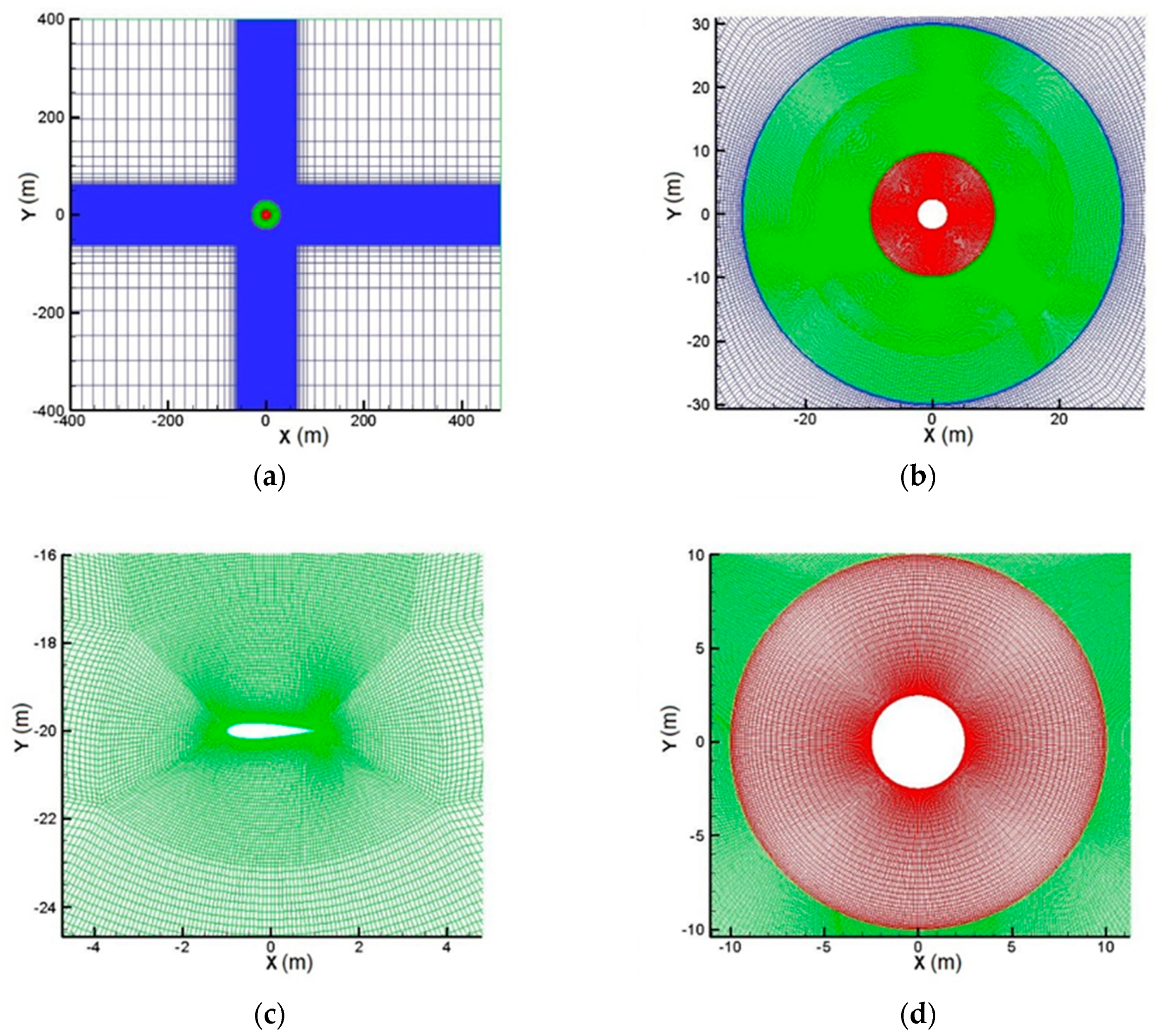
The meshes of the entire flow field, cell zone 2, near a blade, and cell zone 3 are illustrated in Figure 5a–d, respectively. The numbers of grids in cell zones 1, 2, and 3 are 32,000, 174,600, and 24,432, respectively. The total number of grids in this 2D SST k-ω simulation is 231,032.
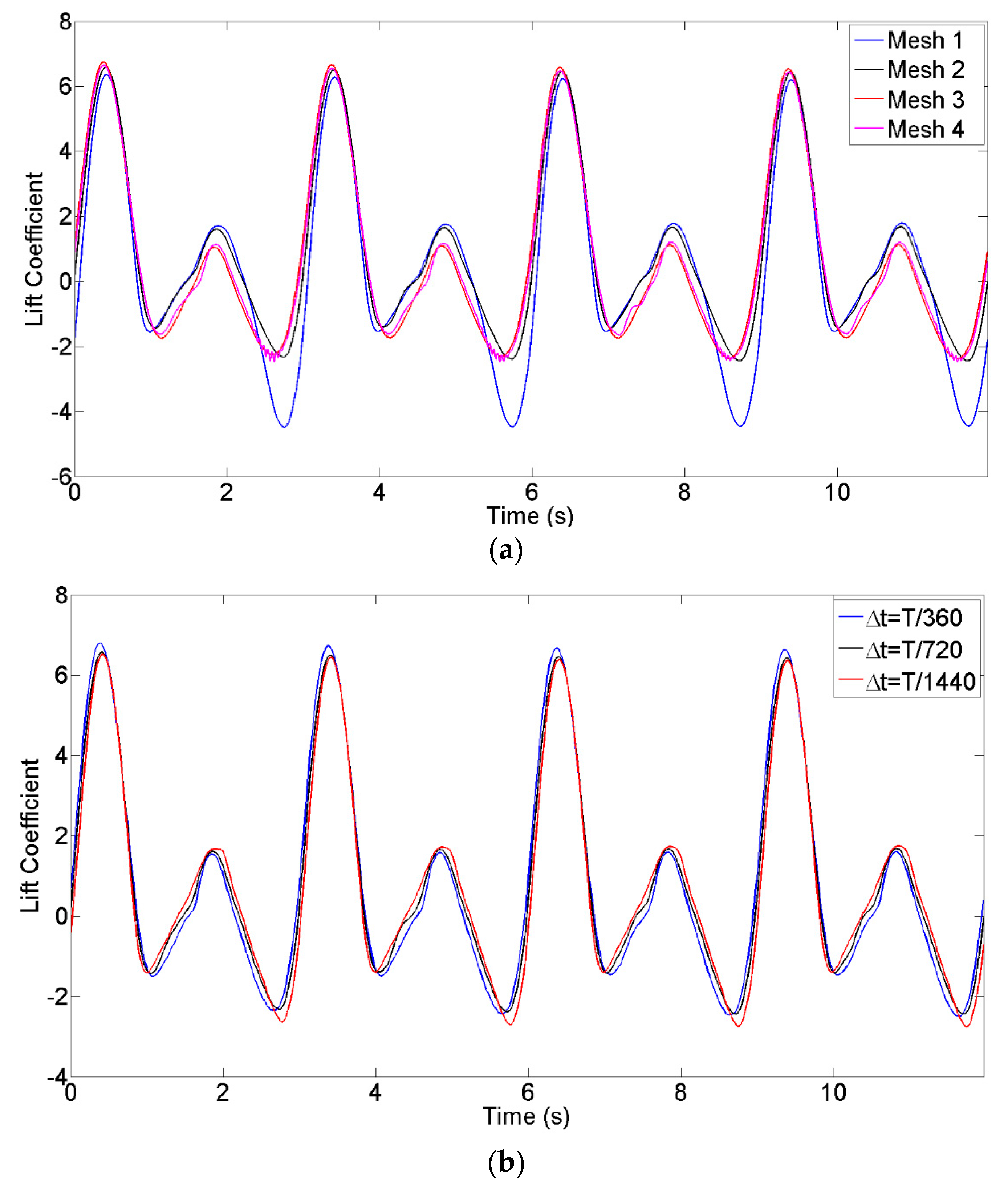
To verify mesh convergence, a mesh sensitivity study is conducted. The wind speed of 20 m/s and the rotational speed of 2.1 rad/s are adopted. Four mesh cases are selected, that is, the total number of the grids is 192,032 (Mesh 1), 231,032 (Mesh 2), 309,032 (Mesh 3), and 349,832 (Mesh 4). The lift coefficients of these four cases are calculated and shown in Figure 6a. The results of Mesh 1 are noticeably different from other results. Mesh 2′s results are very close to those of Mesh 3 and Mesh 4, and the difference between Mesh 3 and Mesh 4 is negligible. Although the finer mesh with a smaller mesh size would lead to more accurate results, Mesh 2 is adopted in this study considering the trade-off between the computational cost and accuracy.
In addition, three different time steps, namely, Δt = T/360, T/720, and T/1440, are adopted based on Mesh 2. The lift coefficients are shown in Figure 6b. It is shown that the three results are similar and Δt = T/720 is selected in the following simulations. The y-plus of the results obtained by SST k-ω and LES is smaller than 2. For more details, please refer to the works of [5,8].
In the 2.5D LES model, the 2D mesh introduced above is extruded by 4 m with 40 layers in the vertical direction (z). Translational periodic conditions are applied on the top and bottom boundaries. Specifically, the blades and tower are infinitely long, and the influences of the finite span are ignored. The total number of grids is 9,241,280, which is much larger than that of the 2D SST k-ω case and is extremely computational intensive. In this CFD simulation, the inflow velocity is selected as 10 m/s, and no turbulence in the inflow is considered. The tip speed ratio λ(ωR/V∞) has a determinant influence on the aerodynamic forces [1,27]. Thus, two cases, namely λ = 1 and λ = 3, are considered in the simulation. The rotation speeds are 0.5 and 1.5 rad/s.
3.2. Wind Load Simulation Result
The simulated wind loads, including wind pressures and aerodynamic forces obtained from the two models above, are compared in this subsection. The 2.5D LES is actually a 3D model. Thus, the results are averaged through the thickness to compare them with those from the 2D SST k-ω simulation. The pressure coefficient Cp, the normal force coefficient Cn, and the tangential force coefficient Ct are defined by the following equations.
where p, Fn, and Ft are the wind pressure, the normal force, the tangential force, and the moment, respectively; c is the chord length; ρ is the density of air; and V∞ is the inflow velocity. The reference point has to be given, which usually takes the point at c/4 away from the leading edge in the chord line, to determine the force and moment by integrating wind pressures over the cross section of the blade. The normal force Fn is then defined as the component of the aerodynamic force perpendicular to the chord, from outside to inward; the tangential force Ft is the component of aerodynamic force along the chord line and pointing from the trailing edge to the leading edge; and the moment refers to the reference point with the counter-clockwise moment as positive in this study.
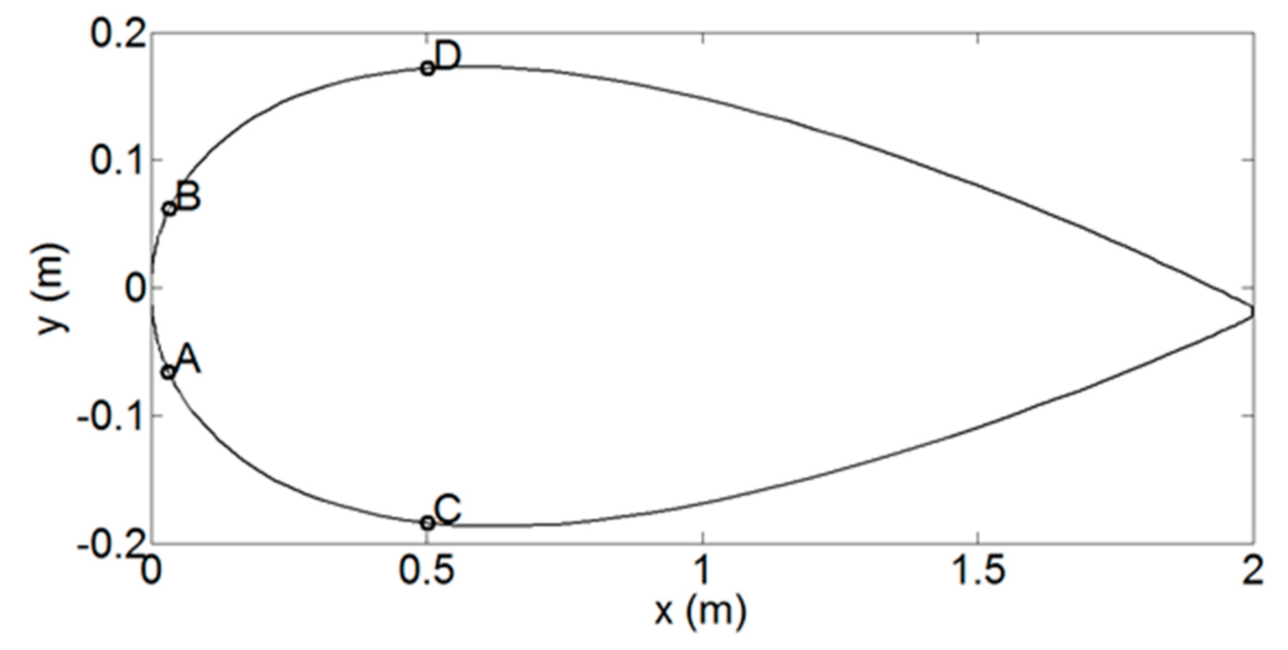
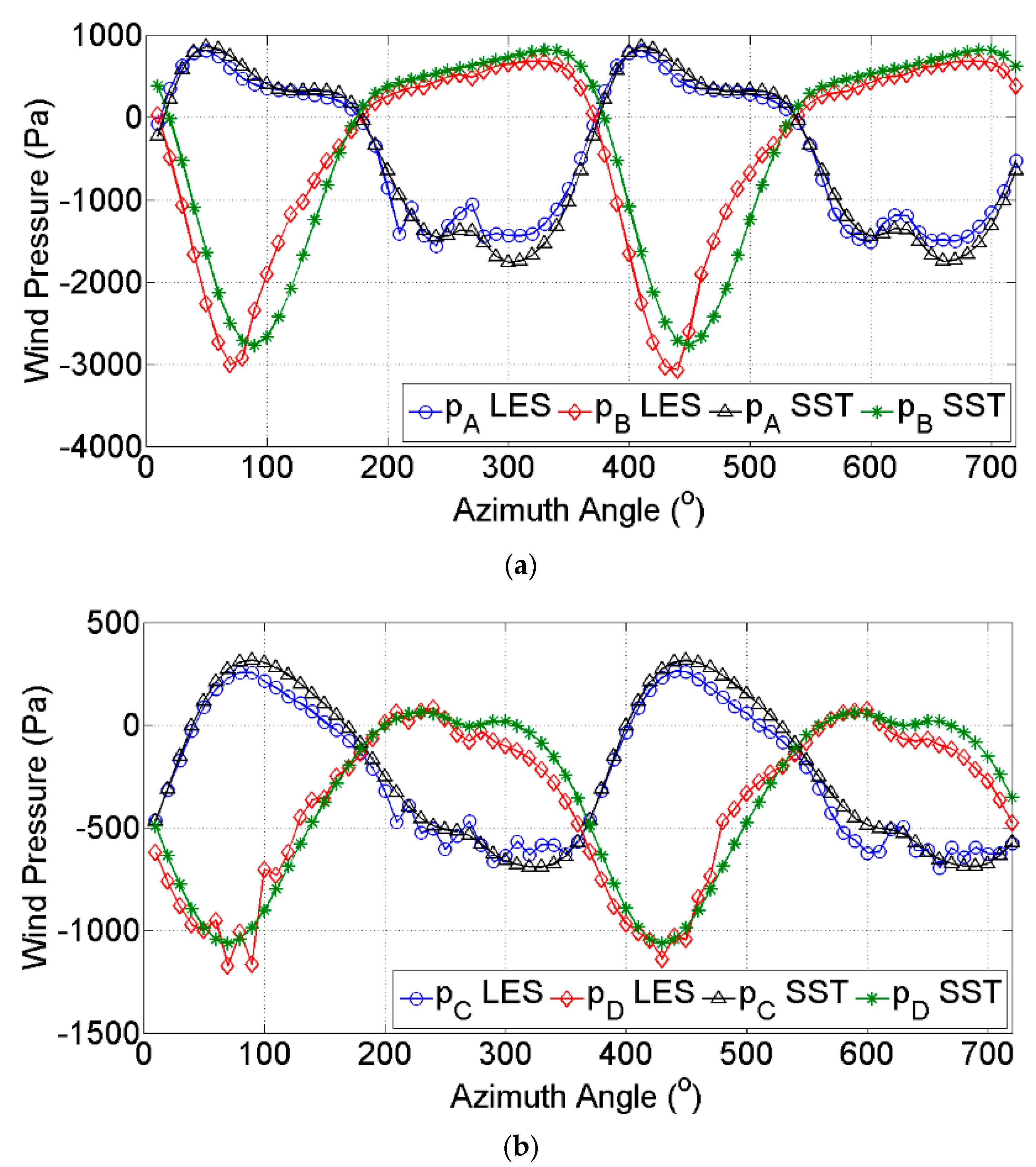
The simulated wind pressures by the two methods are compared in two aspects: one is the time- varying wind pressures at the chosen points of the blade section, and the other is the pressure distribution over the cross section of the blade at different azimuth angles θ. The cross section of the blade is shown in Figure 7, in which four points, namely, A, B, C, and D, are chosen.
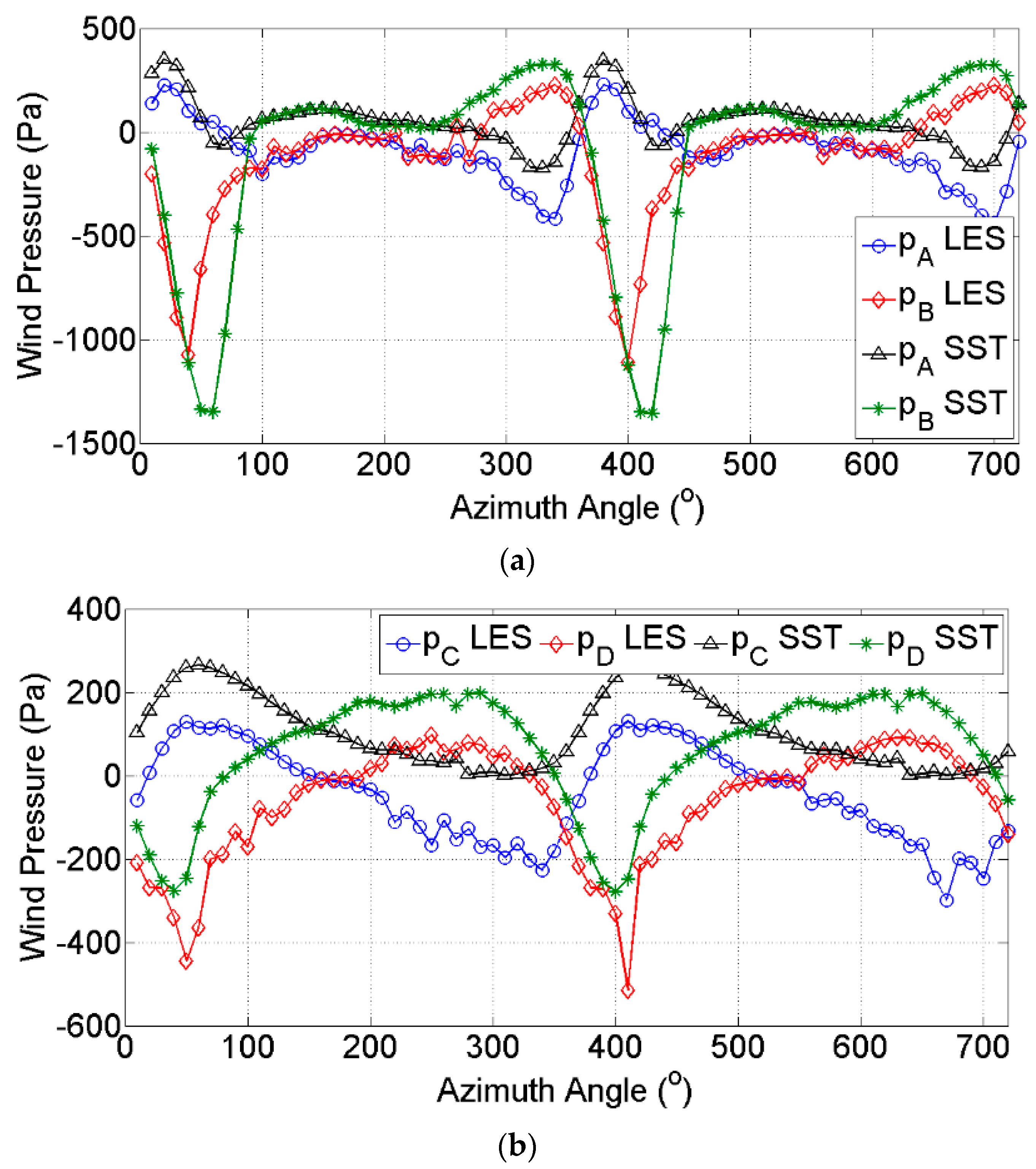
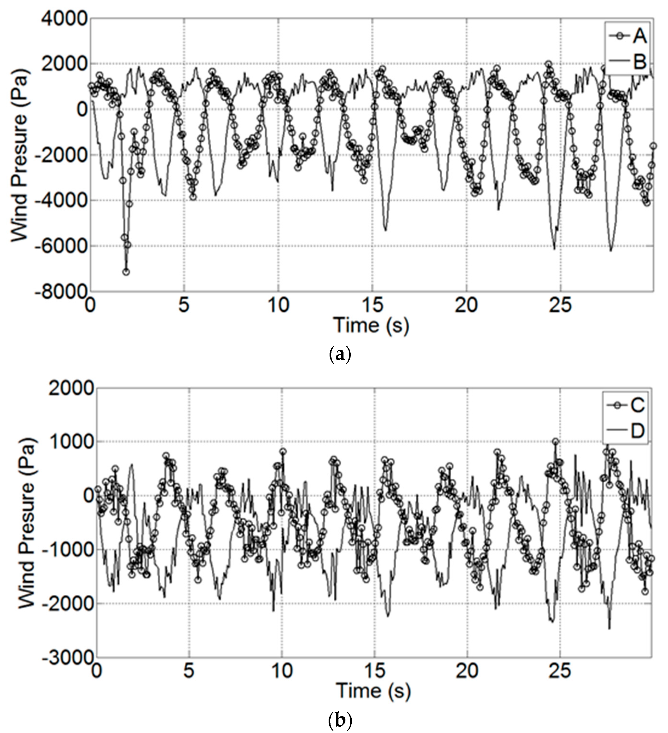
The wind pressure time histories at the four points are shown in Figure 8 for λ = 1 and Figure 9 for λ = 3. The wind pressure time history is periodical at 360° because of the rotation of the VAWT and the mean wind speed. Given the rotation of the VAWT, the wind pressures at points A and B are not equal even at the zero azimuth angle. The same condition is found for points C and D. For λ = 1, the absolute magnitudes of the pressures at A and B increase with the increase in azimuth angle from zero. When the azimuth angle reaches a certain value, the magnitudes decrease. For example, the pressure at point B given by LES decreases at approximately θ = 40°, whereas that by SST k-ω simulation decreases at nearly θ = 60°. The largest pressure differences between A and B given by the two models coincidently appear at these azimuth angles. The pressures at A and B then decrease to around zero at θ = 180° for the LES and SST k-ω simulations. In the downwind side, the pressures at A and B retain a small value within a range of azimuth angle between 180° and 250°. After this range of azimuth angle, the pressure at point A becomes negative and the pressure at point B becomes positive. The reason is that in the azimuth angle range of 180°–360°, the upwind surface of the blade becomes the downwind surface, and vice versa. The variation in the pressures at C and D is similar to that in the pressures of A and B. Moreover, the pressures given by the SST k-ω simulation at the four points have evident shifts to the positive pressure, whereas the pressure difference between A and B and that between C and D are close to the corresponding results of LES.
For λ = 3, the results from the two models are much closer to each other than for λ = 1. For both results, the pressures at A and C are positive in the range of θ ∈ [0°, 180°] and become negative in the range of θ ∈ [180°, 360°]. By contrast, the pressures at B and D are negative in the range of θ ∈ [0°, 180°] and become positive in the range of θ ∈ [180°, 360°]. Notably, the maximum pressure difference between A and B (or between C and D) in this case appears at a larger azimuth angle than the corresponding azimuth angle for λ = 1.
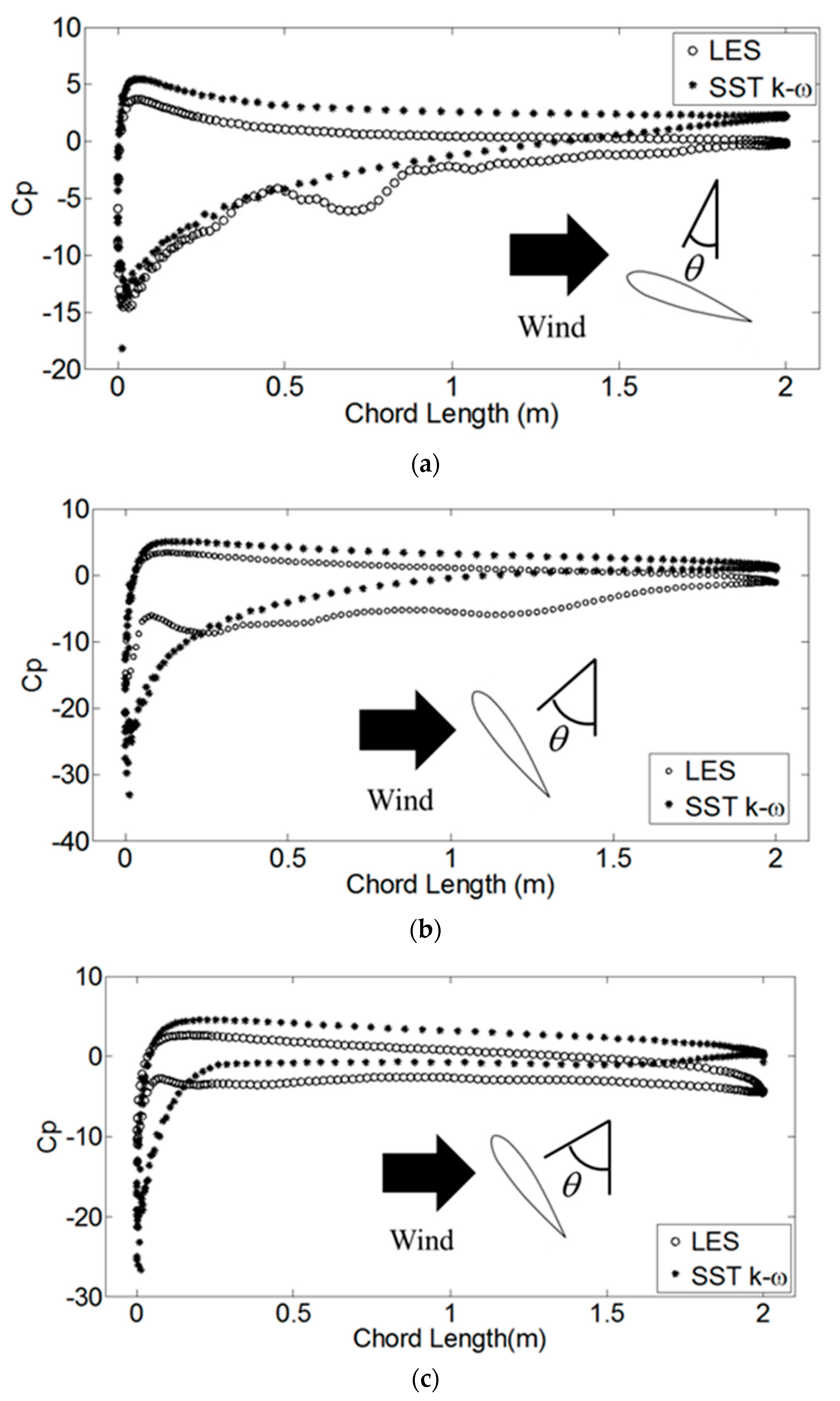
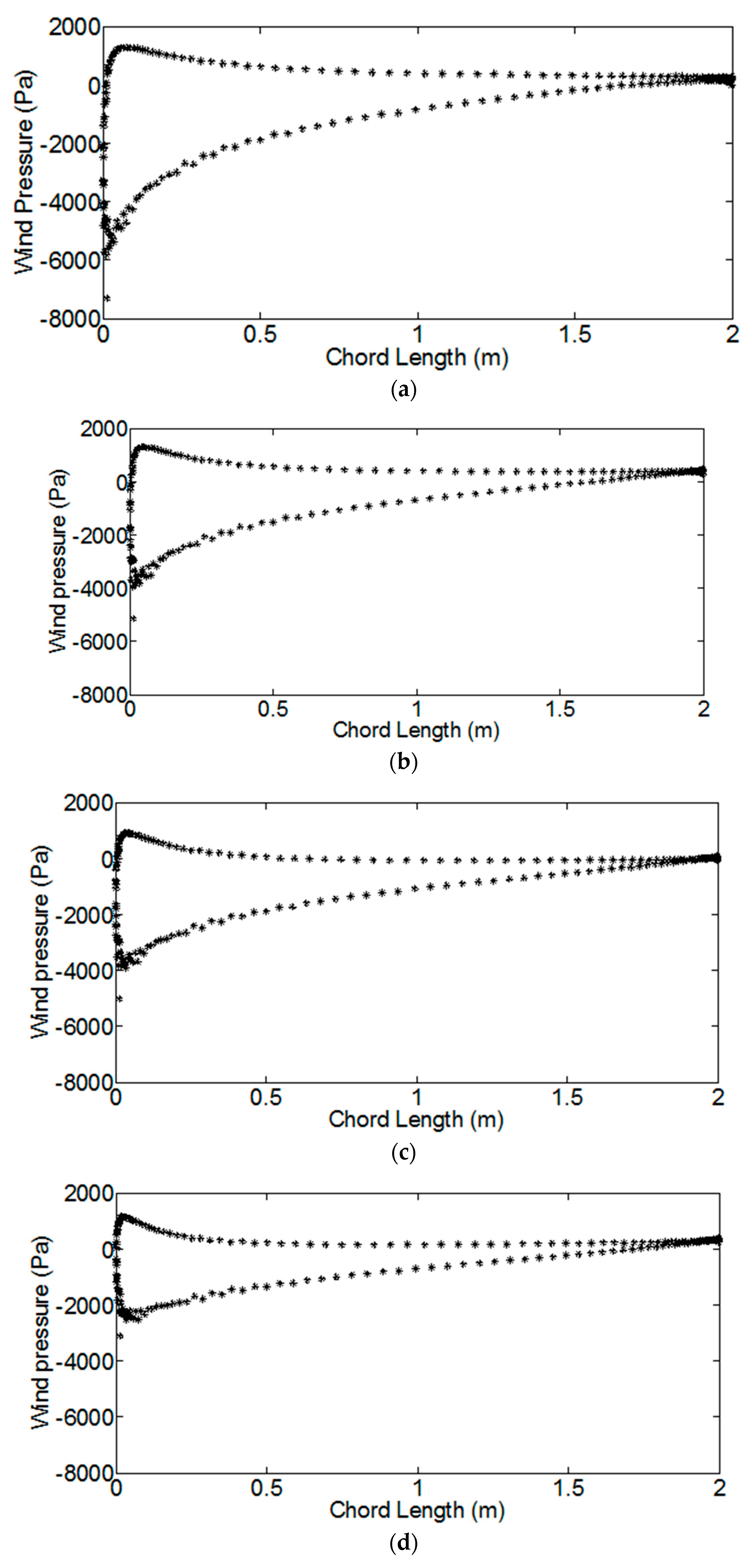
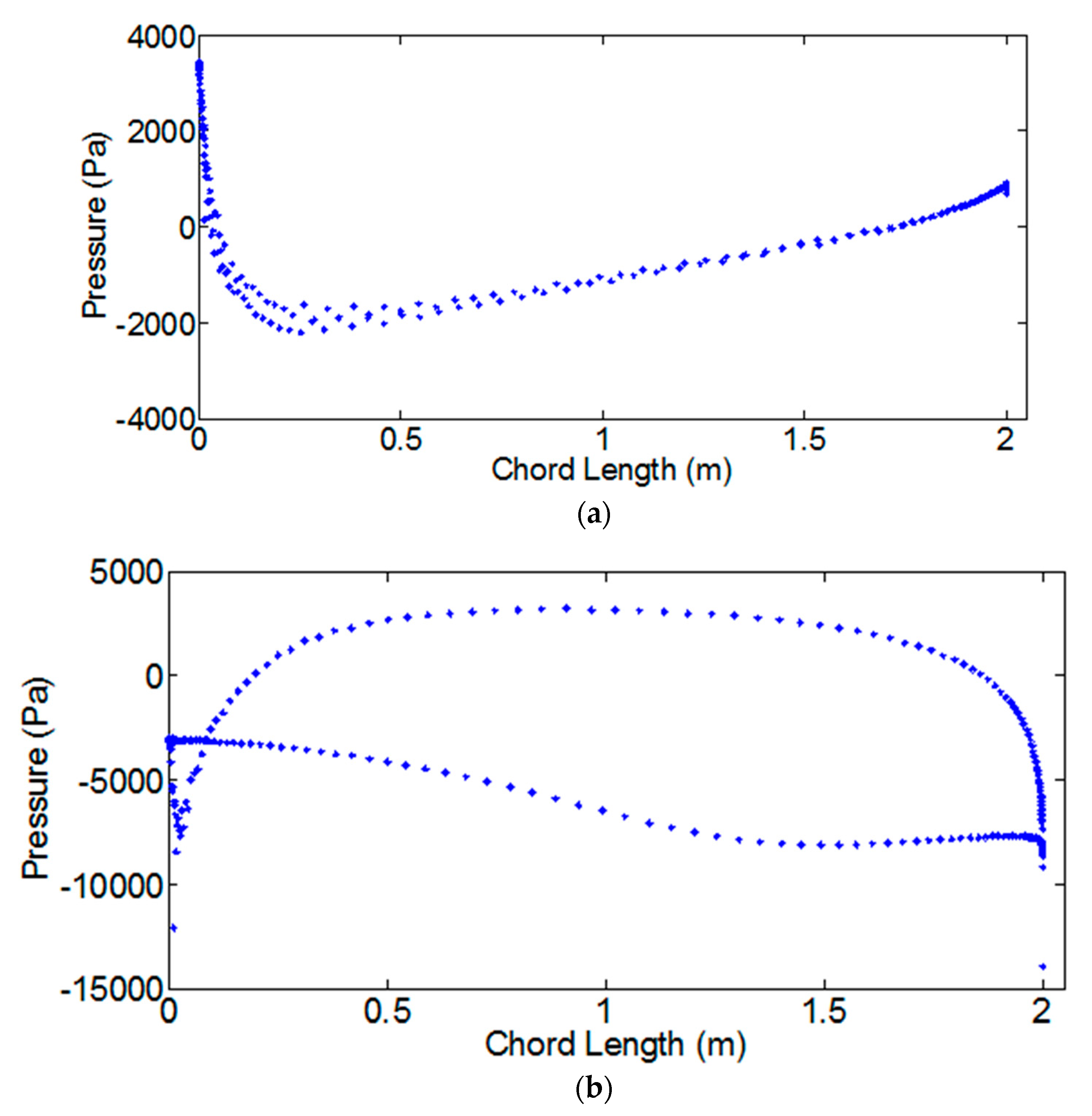
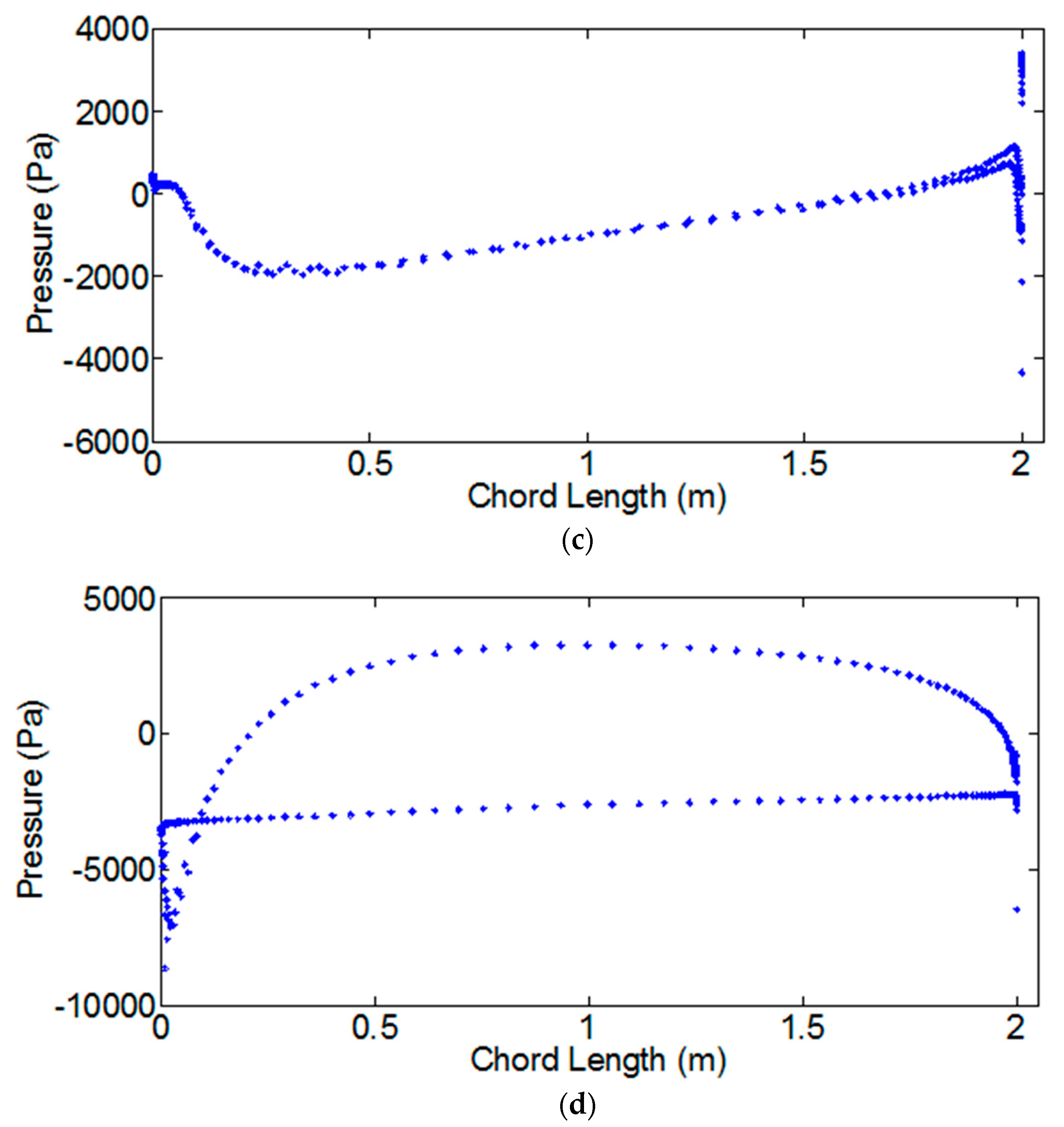
The pressure distribution over the cross section of the blade at a given azimuth angle θ is presented in Figure 10 for λ = 1. In the figure, the abscissa is the chord length of the blade, from the leading edge at 0 m to the trailing edge at 2 m, and the ordinate is the wind pressure on the blade. For θ = 30°, the pressure distribution patterns obtained by the two methods are similar. The pressures are positive on the outside surface of the blade and negative on the inside surface in general. The pressure difference mainly occurs on the leading edge and decays to zero at the trailing edge, which is consistent with the aerodynamics analysis [44]. The wind pressure given by the SST k-ω simulation has an evident shift to the positive pressure side compared with the results by LES. When θ = 50° (Figure 10b), the pressure distribution patterns from the two methods are quite different. The result given by SST k-ω remains similar to that at θ = 30°, but the negative pressure given by LES decays quickly at the leading edge and becomes relatively flat nearly in the entire upper surface (inside surface of the vertical blade). At θ = 70°, the negative pressures obtained by the two models decay quickly near the leading edge and become flat throughout the chord line.
When the flow separation occurs, the pressure in the separation area is negative [44]. The phenomenon shown in Figure 10 can be explained as follows. When θ = 30°, flow separation does not occur for both models. Thus, the results of the two models are similar. When θ = 50°, flow separation occurs in LES, but not in SST. Thus, the results of LES become flat. When θ = 70°, flow separation occurs in both models.
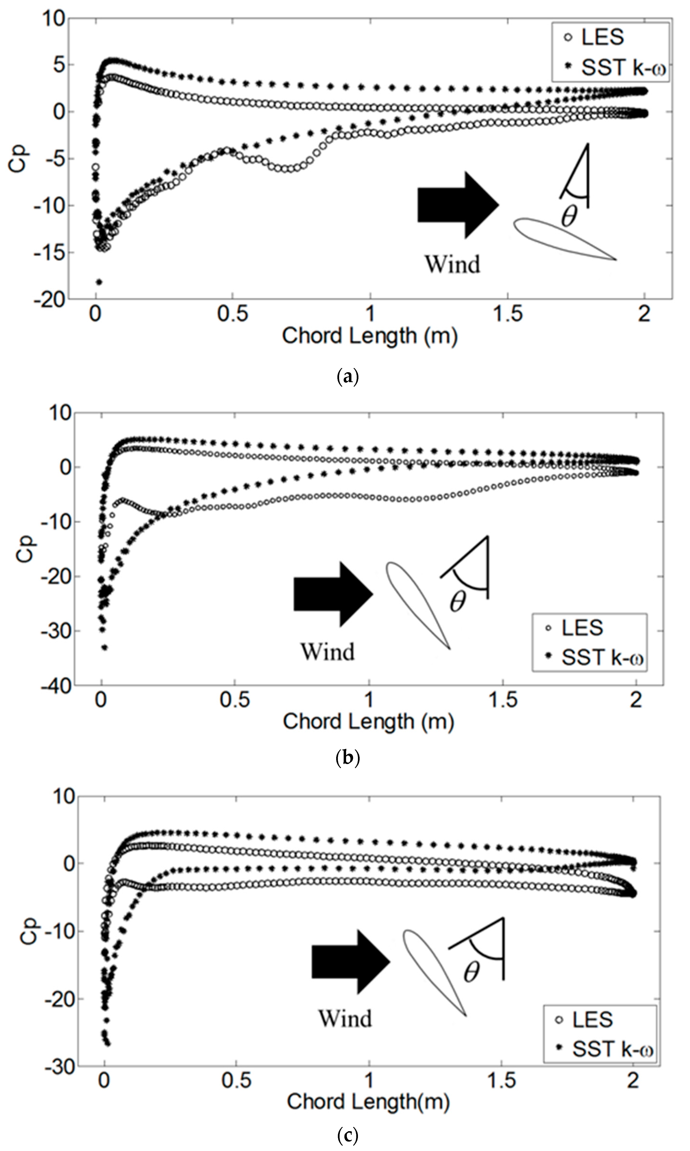
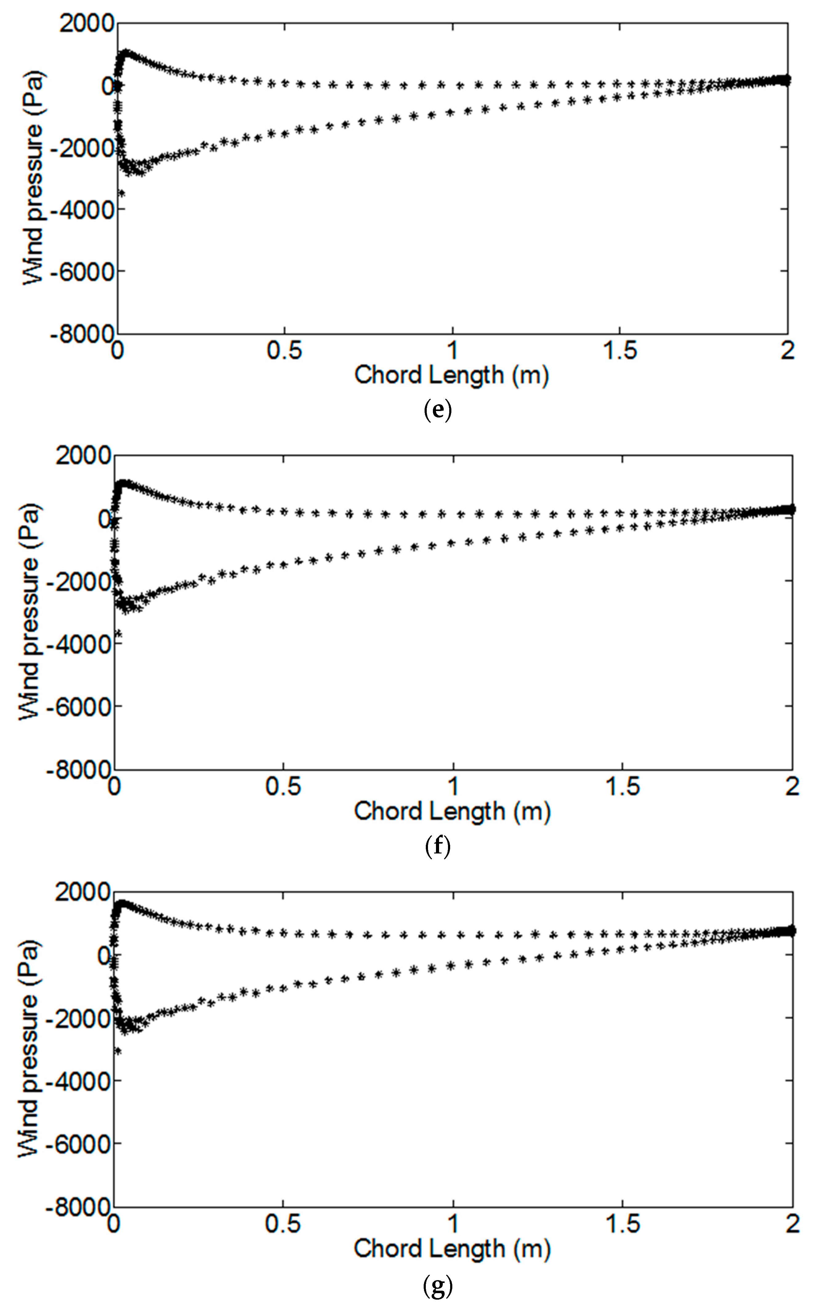
The pressure distributions with a large tip speed ratio λ = 3 are shown in Figure 11. When θ = 60° (Figure 11a), the two results match well. When θ = 105° (Figure 11b) and θ = 130° (Figure 11c), slight differences can be observed. One probable reason is that the largest relative angle of attack is smaller than that in the case of λ = 1. Therefore, flow separation has a low probability of occurring when λ = 1. The main difference between LES and SST k-ω is the prediction of the flow separation. Thus, the results given by the two models are similar for λ = 3.
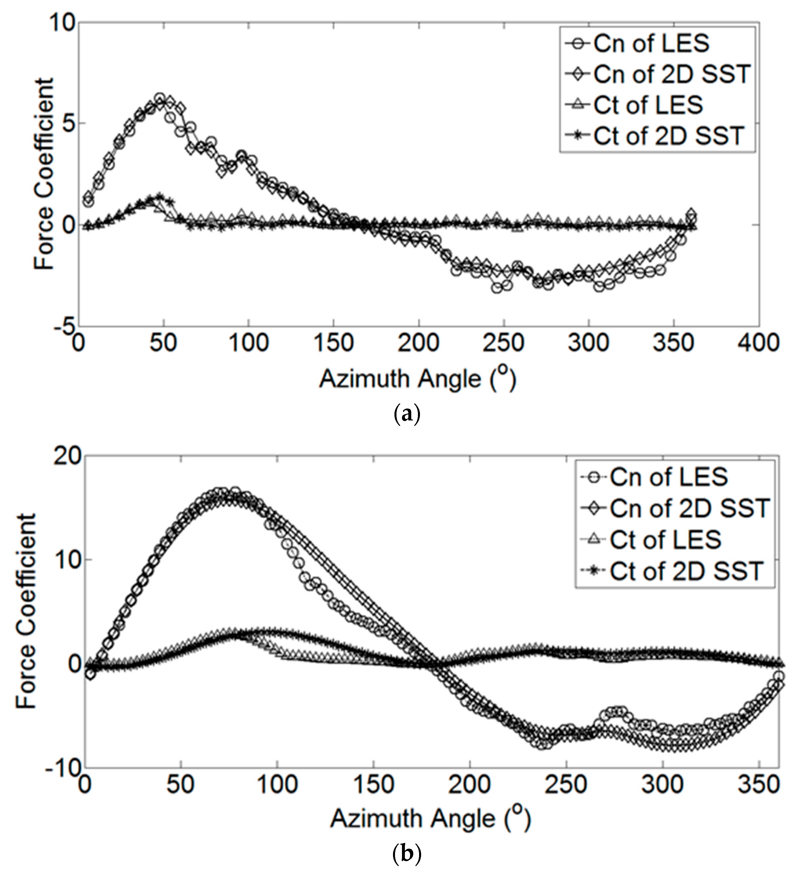
Aerodynamic forces, such as tangential forces, acting on the blade are required to calculate the wind-generated power. These forces can be obtained by integrating the wind pressures over the cross section of the blade. Furthermore, the normal force coefficient Cn and the tangential force coefficient Ct can be obtained from Equations (5) and (6) and used for comparison.
The computed Cn and Ct against the azimuth angle are shown in Figure 12. The force coefficients obtained by the two methods match well for λ = 1. The reason is that the aerodynamic forces are determined by the pressure difference between the upper and lower surfaces. A small difference is observed for λ = 3 in terms of azimuth angles, probably owing to the different estimations in flow separation zones by the two methods. Given that the pressure differences obtained by the two methods match well, the resulting aerodynamic forces are similar. The normal force is much larger than the tangential force. Thus, the normal force is dominant in the structure analysis. In summary, the 2D SST k-ω method is an acceptable alternative to the 2.5D LES method in terms of the accuracy of the results and the efficiency of computation.
4. Wind Loads on the Entire VAWT
The wind pressures on the blade and the aerodynamic forces on the entire VAWT, considering the interference among all the structural components and different wind conditions, are required to conduct the fatigue and ultimate strength analyses of the VAWT. The 2D CFD simulation is performed for the nine selected cross sections (Table 1), and the SST k-ω turbulence model is adopted. The spatial wind loads are interpolated from these discrete sectional results.
4.1. Wind Speed Simulations
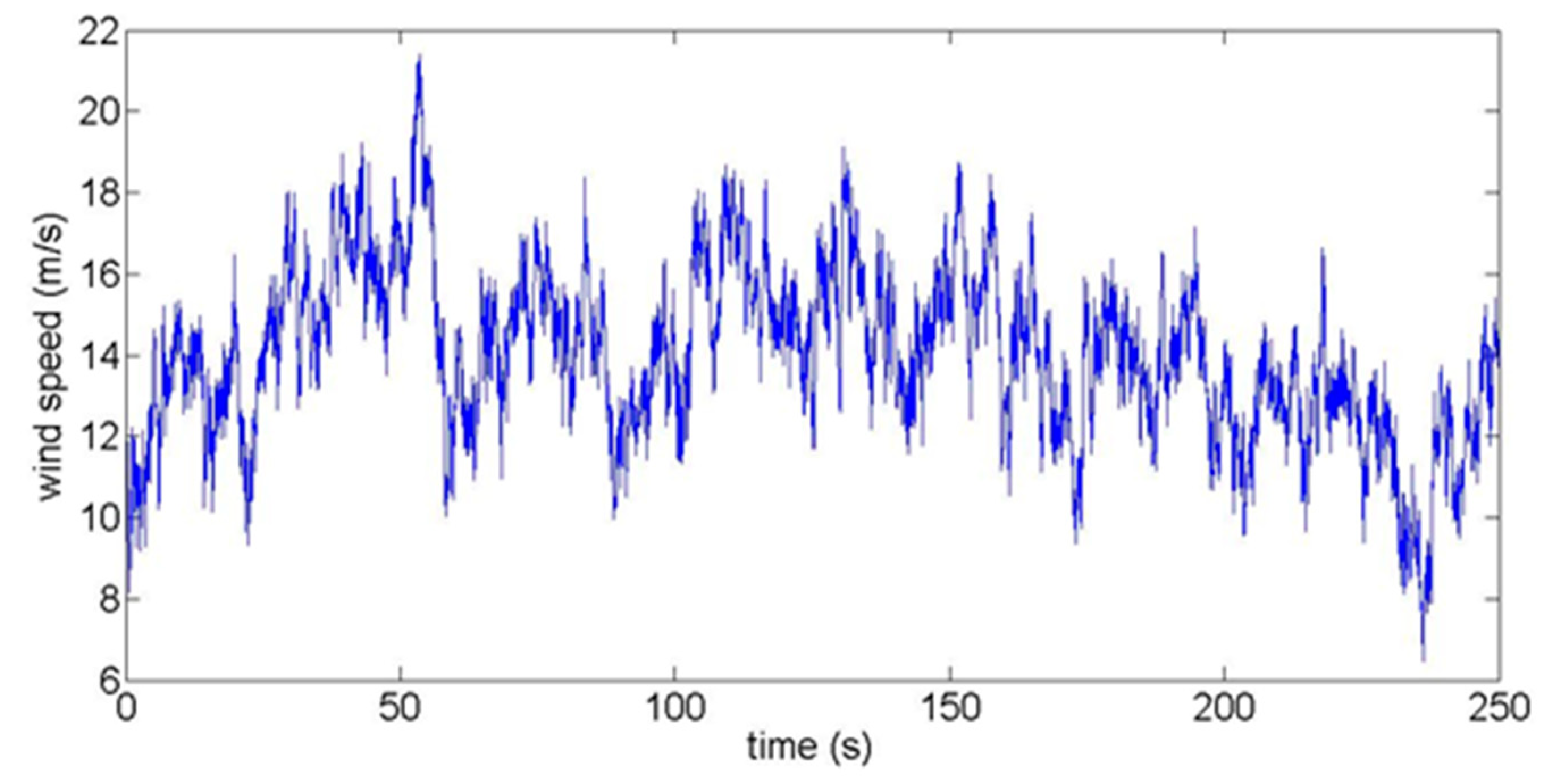
The inflow wind speeds and mesh grids in each section must be given from the entire wind field simulated to conduct the 2D CFD simulation for the selected cross sections of the VAWT. The inflow wind speeds in the nine cross sections are simulated by the strip method introduced in Section 2. The wind speed time histories in the nine cross sections are simulated by taking the mean wind speed of 14 m/s at the hub height, and the wind speed time history of Sec 4 is shown in Figure 13. The wind speed time history contains mean and turbulent wind speed components.
4.2. CFD Simulation Strategy
The CFD simulation strategy and the mesh grids of Sec 7 are introduced in Section 3.1. For other cross sections, the differences lie in cell zones 2 and 3. In these cross sections, the blades and upper/lower arms are modeled in cell zone 2, and the tower is modeled in cell zone 3. Similarly, cell zones 1 and 3 are stationary, and cell zone 2 is a rotating ring. However, the main arms in Sec 4 are modeled in cell zone 3 and cell zones 2 and 3 are rotating. The structural components of the VAWT are all modeled as wall boundaries. The diameter of the vertical links is small (0.2 m). Thus, they are excluded in the CFD simulation.
The grid numbers of the nine cross sections are listed in Table 2. The validity of these mesh grids is verified by the near-wall y-plus values, which are given in Section 4.3 and Section 4.4.
In this study, the VAWT is rotating at 2.1 rad/s. The mean wind speed at the hub is 14 m/s. In the extreme wind speed case, the VAWT is parked.
4.3. Wind Loads in Normal Wind Speed
In the operating wind speed region, the VAWT is rotating. Spatially continuous and time-varying wind pressures of the discrete cross sections are obtained in this subsection. The wind pressures on the blade are also calculated.
The wind pressures of the discrete sections are simulated first and then the wind pressure in an arbitrary cross section is obtained by interpolation. The wind pressures on the blade in seven cross sections are time varying (the blades are only presented in Sec 1–Sec 7). The time histories of wind pressures at points A, B, C, and D in Sec 1 are shown in Figure 14. The time histories are in the same phase as those shown in Figure 8 and Figure 9. The wind pressure varies periodically overall as a result of the rotation of the VAWT with some local fluctuations, because the turbulence is considered in the present inflow.
The wind pressures on the blade in Sec 1–Sec 7 at 18.70 s (θ = π/2) are shown in Figure 15. The wind pressure magnitudes in the leading edge of higher sections are generally larger than those of lower sections. The wind pressure magnitude in Sec 4 is smaller than others because of the influence of the main arm. The wind pressure around the blade tail in all cases is nearly equal to zero, which is consistent with the Kutta–Joukouski theorem.
In these simulations, the near-wall y-plus values in Sec 1–Sec 9 are 1.4, 1.4, 1.3, 1.1, 1.4, 1.3, 1.3, 0.5, and 0.4, respectively. All y-plus values are less than 2, which satisfies the near-wall requirement that y-plus should be less than 5 for the SST k-ω model [45].
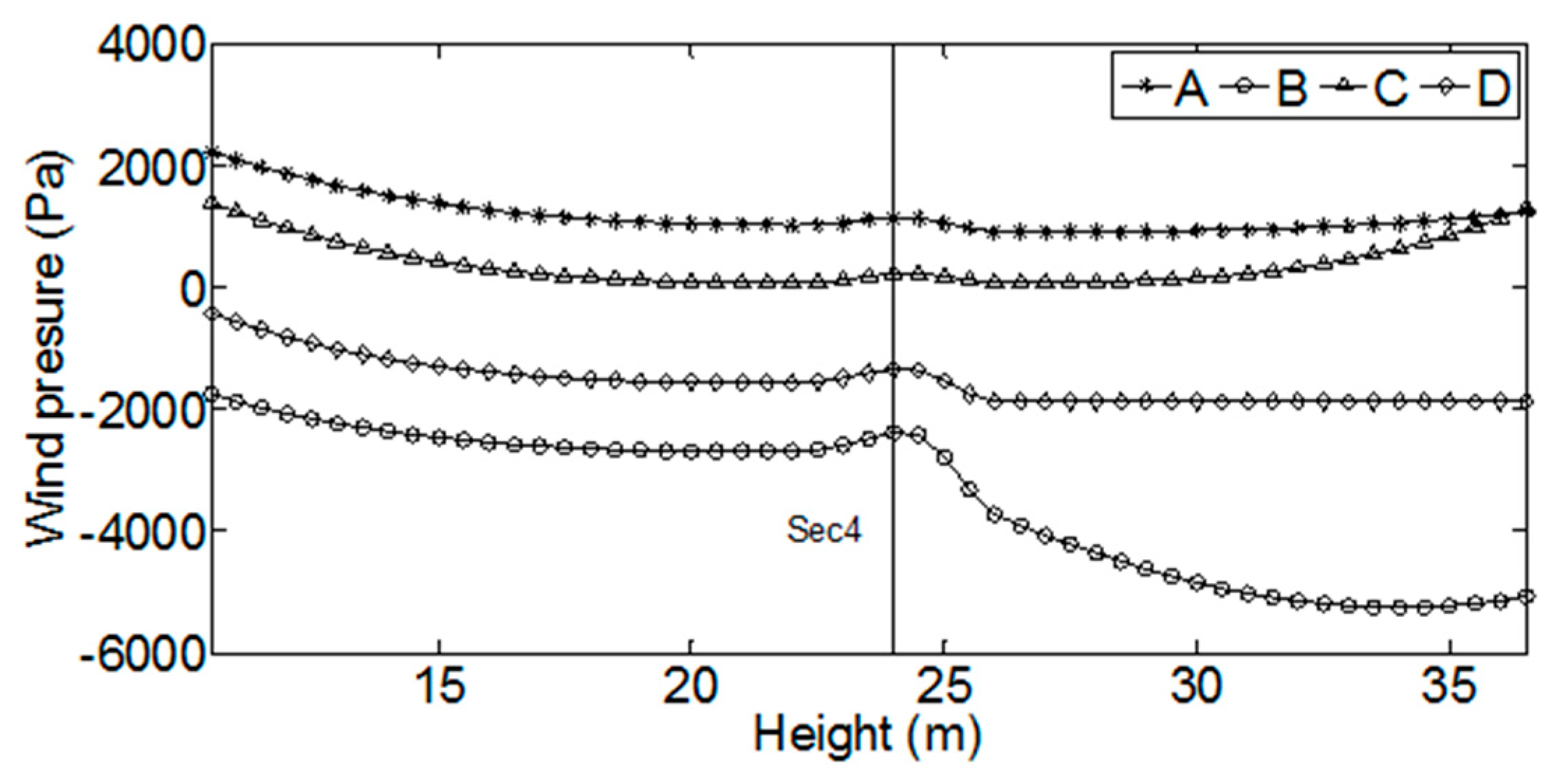
Figure 16 shows the wind pressure profiles of points A, B, C, and D, along the height of the blade, in which the piecewise spline interpolation method is used to obtain the pressures at the height other than Sec 1–Sec 7. Similarly, the negative wind pressure magnitudes at the higher sections are larger than those at the lower sections. The positive wind pressure along the height is relatively flat. The distribution of wind pressures abruptly changes near Sec 4 because of the influence of the main arm.
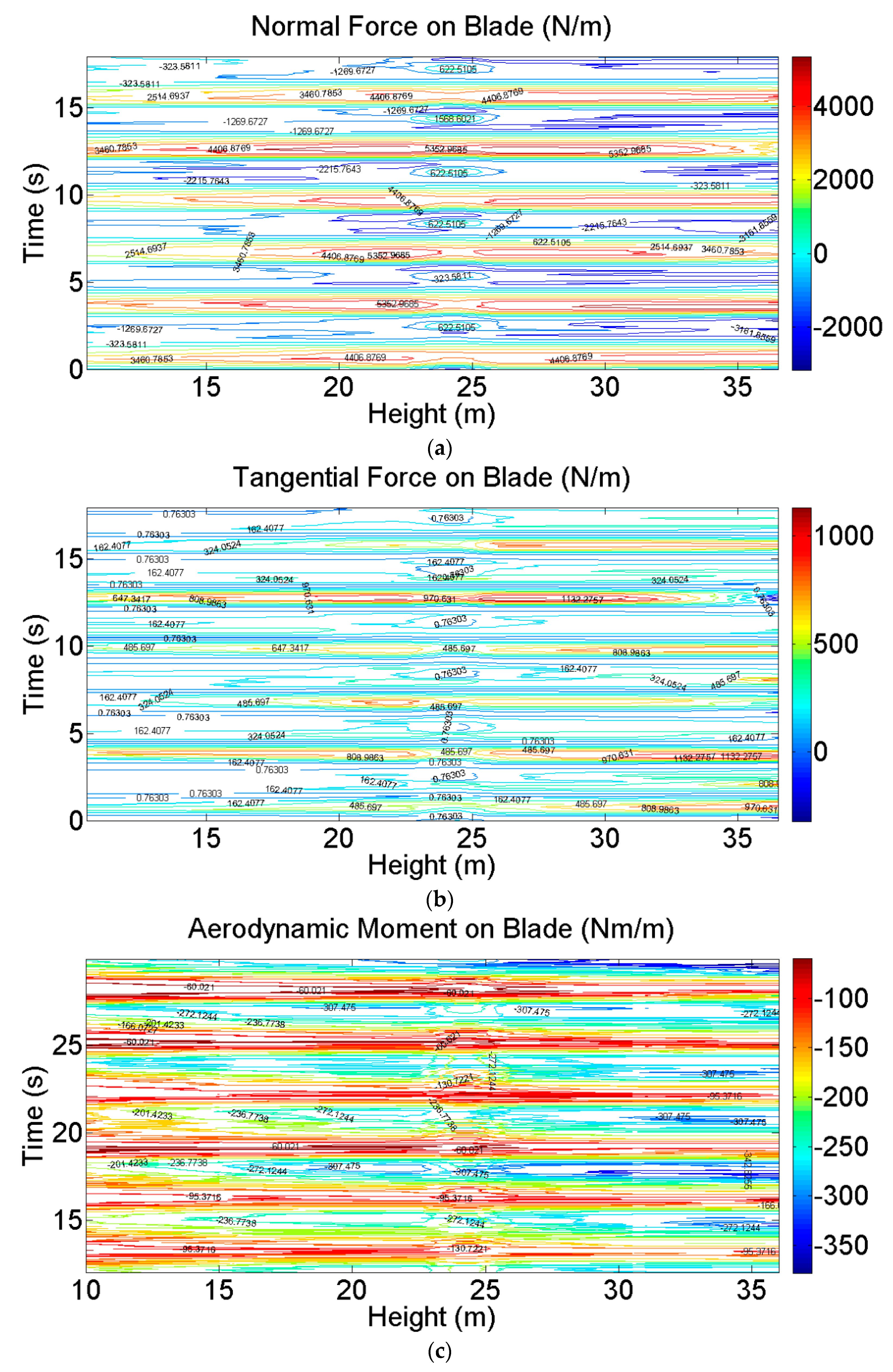
Apart from the blades, other components of the VAWT must also be analyzed. These components are made of steel or reinforced concrete and thus can be modeled by beam elements. Therefore, the aerodynamic forces other than wind pressure are required. Aerodynamic forces, including normal force, tangential force, and moment, can be obtained by integrating the wind pressures over the surfaces of the components. The time-varying aerodynamic forces on the blade per unit length along the height of the blade are shown in Figure 17. Notably, the blade is installed from 10.5 m high above the ground to 36.5 m high at the top (Figure 2). The aerodynamic forces vary with the change in height. The force is small when it is close to the ground. In addition, the tangential force is much smaller than the normal force. The normal and tangential forces decrease at the mid-span of the blade because of the existence of the main arm. The forces are periodical as a result of the rotation of the rotor.
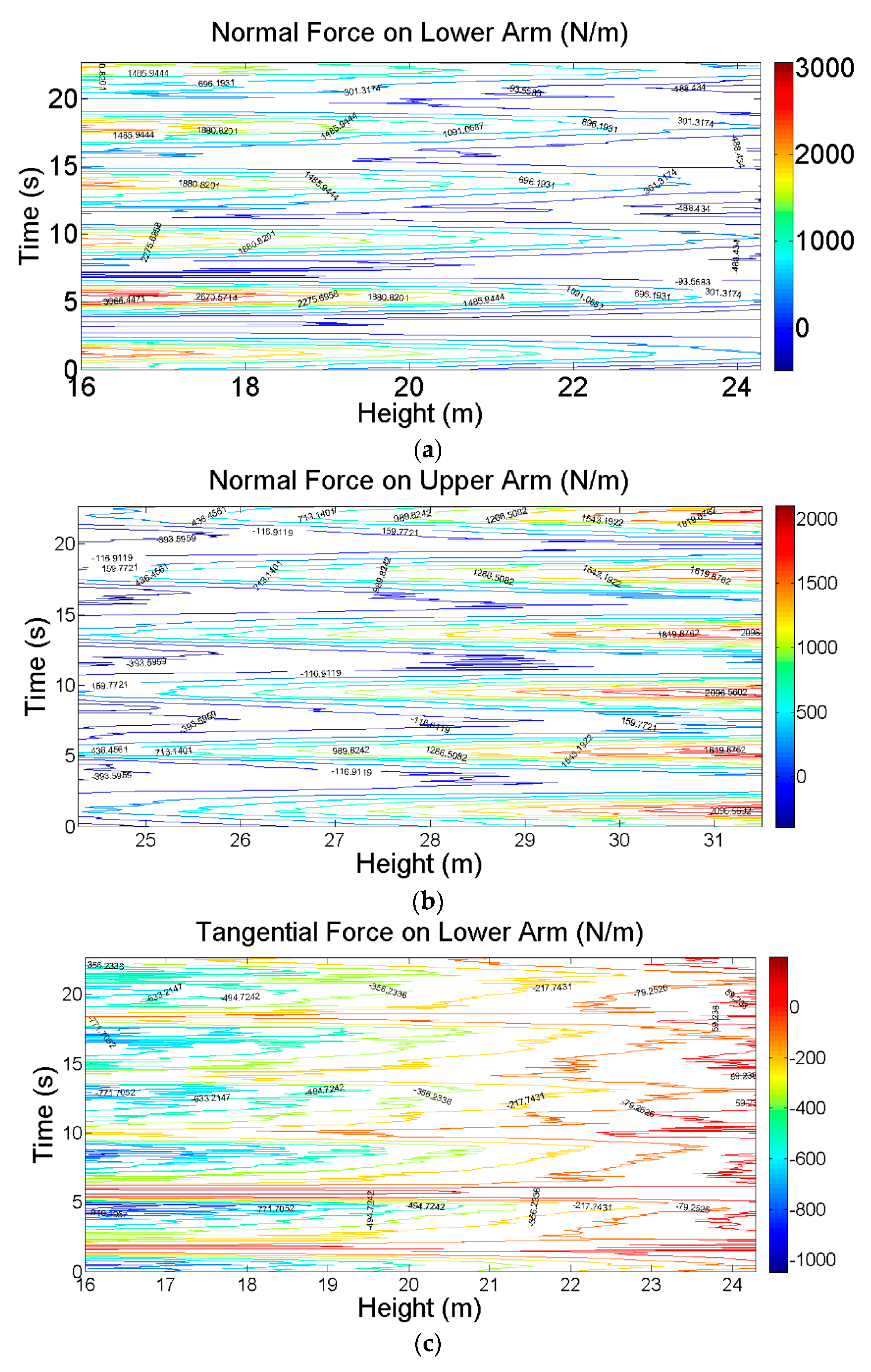
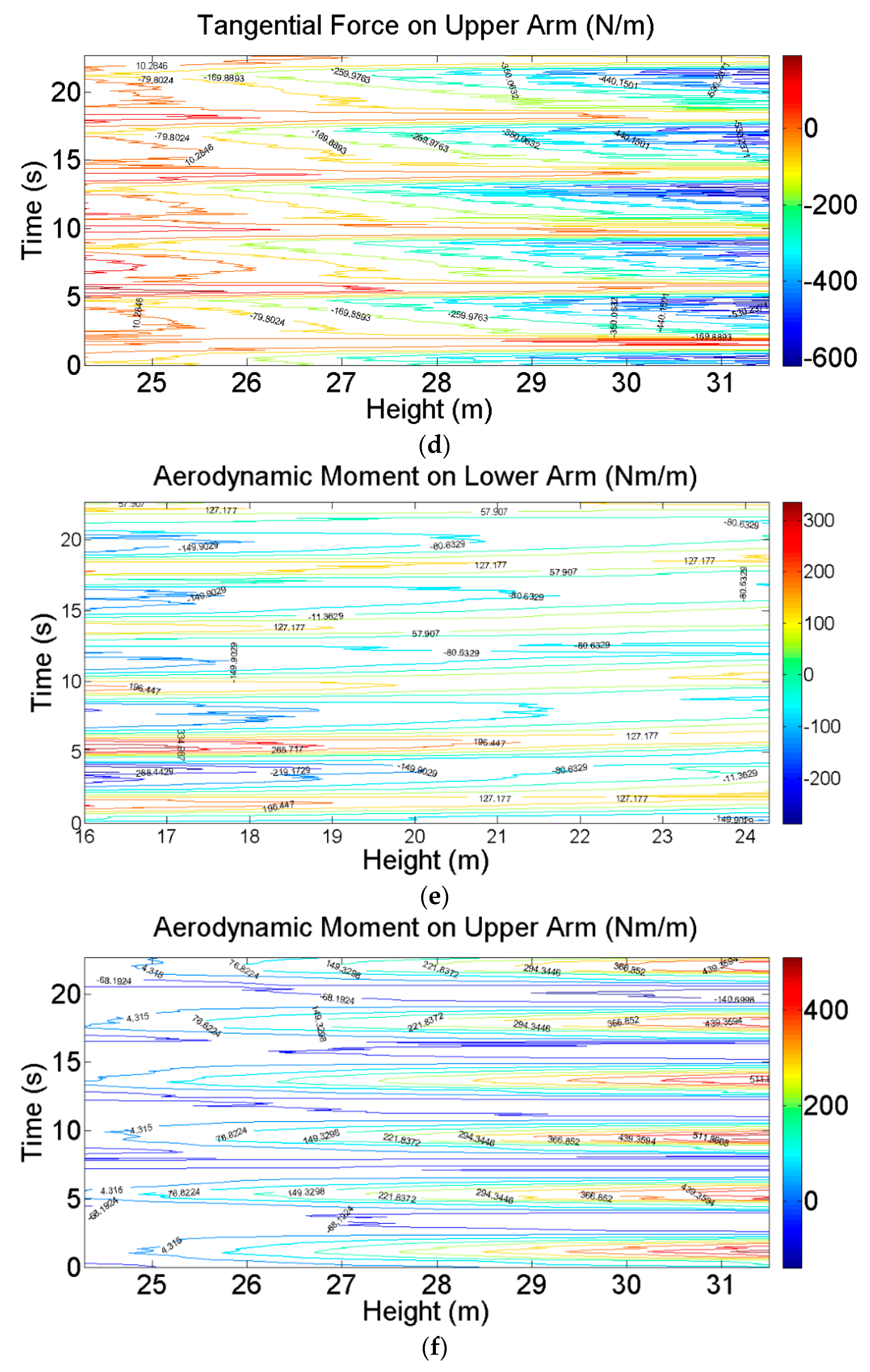
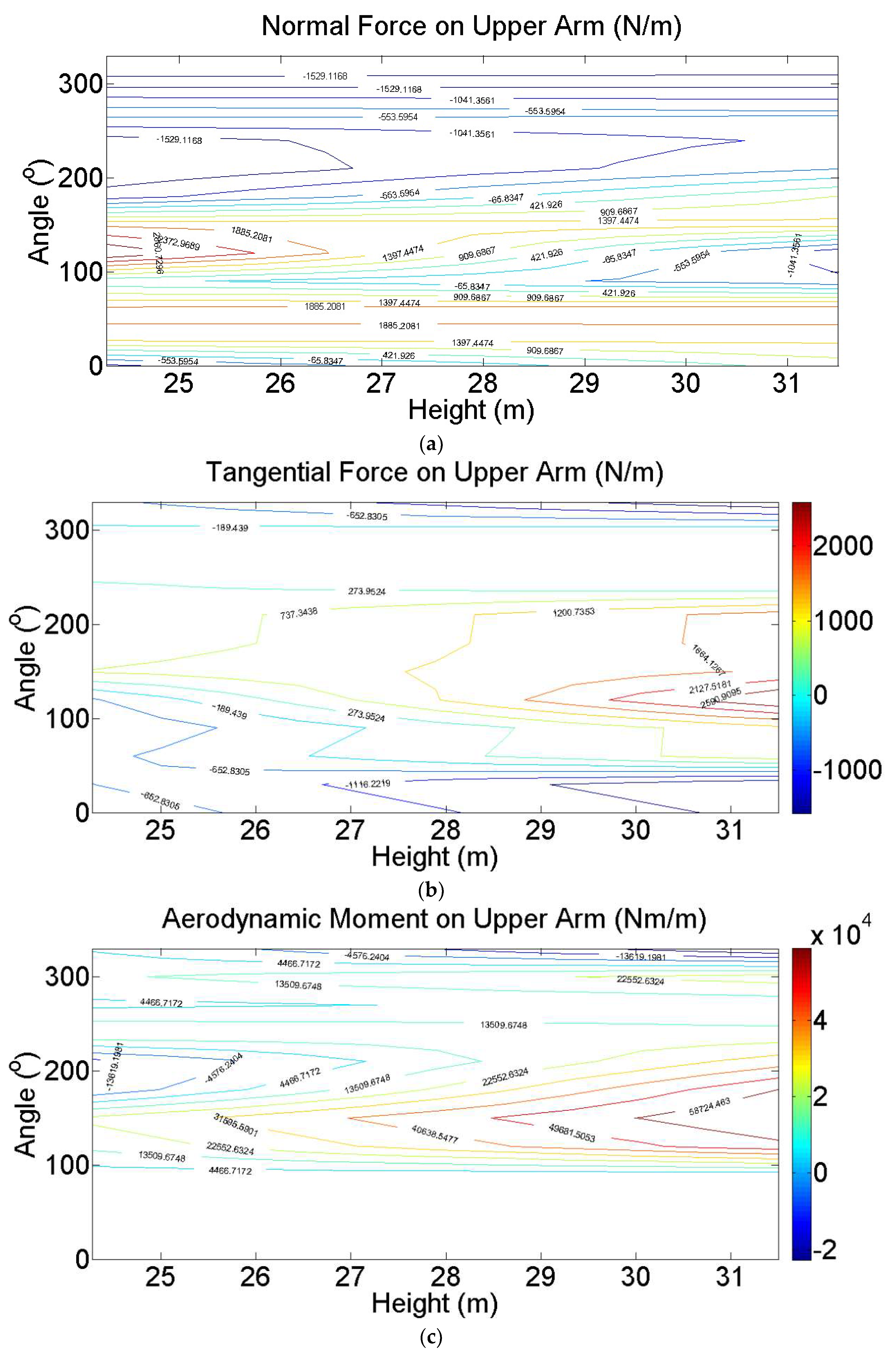
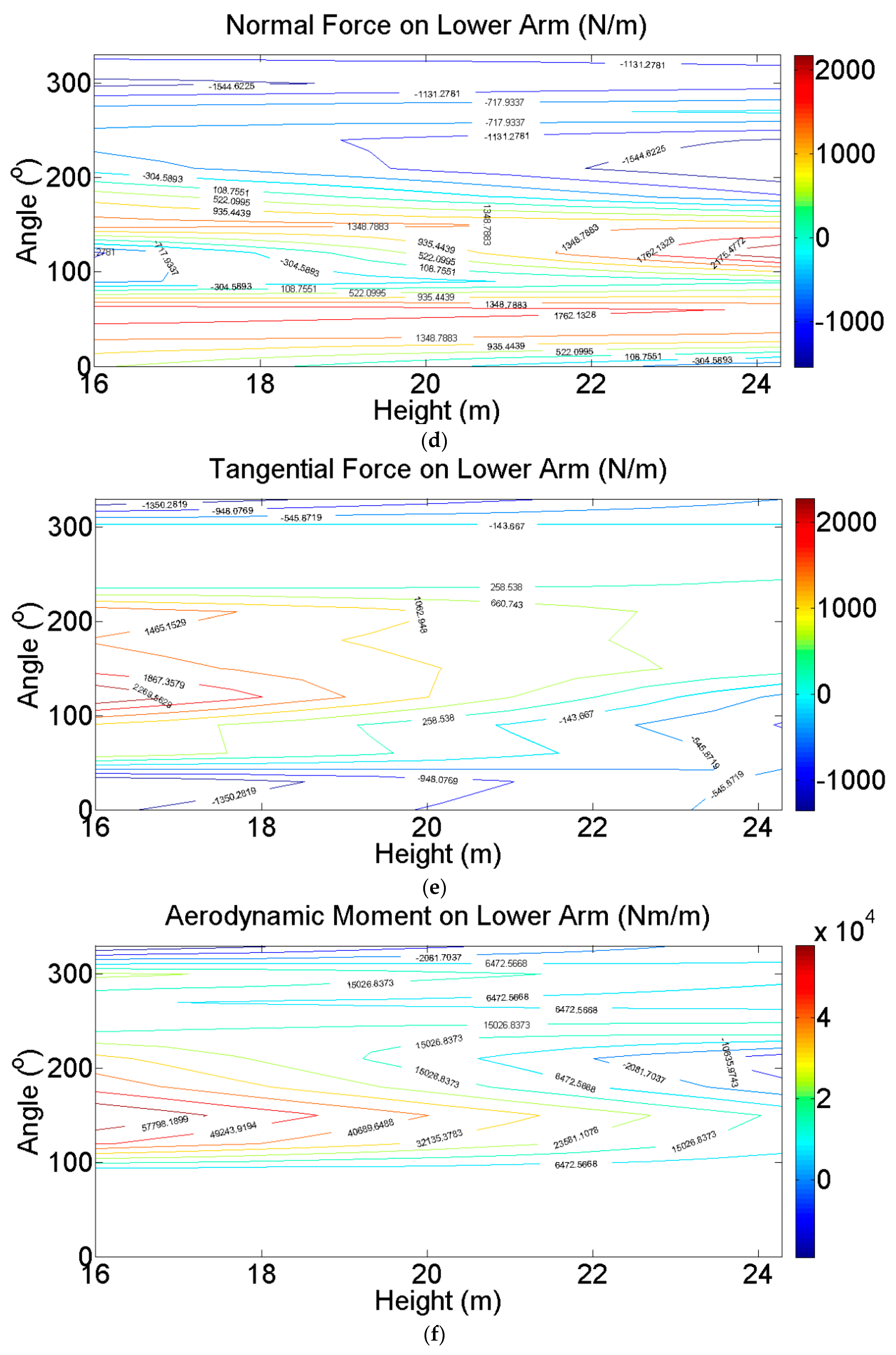
The aerodynamic forces and moment of the upper and lower arms are also simulated. Unlike the blades, which are vertical, the upper and lower arms are tilted. The lower arm is installed from 16 m high above the ground at the blade end to 24.28 m high at the tower end; the upper arm is from 24.28 m to 31.50 m (Figure 2). Given that the CFD simulations are conducted in the horizontal planes, the simulated aerodynamic forces and moment on the upper and lower arms are in the horizontal section. These aerodynamic forces at a given horizontal section are represented by the normal and tangential forces. The normal force points to the center of the rotor, whereas the tangential force is orthogonal to the normal force and along the tangential direction on the section where the upper and lower arms are rotating. The moment is calculated along the geometrical center of the horizontal section. The spatial continuous and time-varying aerodynamic forces per unit length of the lower and upper arms are shown in Figure 18. The aerodynamic force at the tower end is always smaller than that at the blade end. This is because the wind speed near the tower is much smaller than that near the blade. Moreover, the tangential forces of the upper and lower arms are negative most of the time, especially at the blade ends. Thus, the upper and lower arms obstruct the rotation of the VAWT.
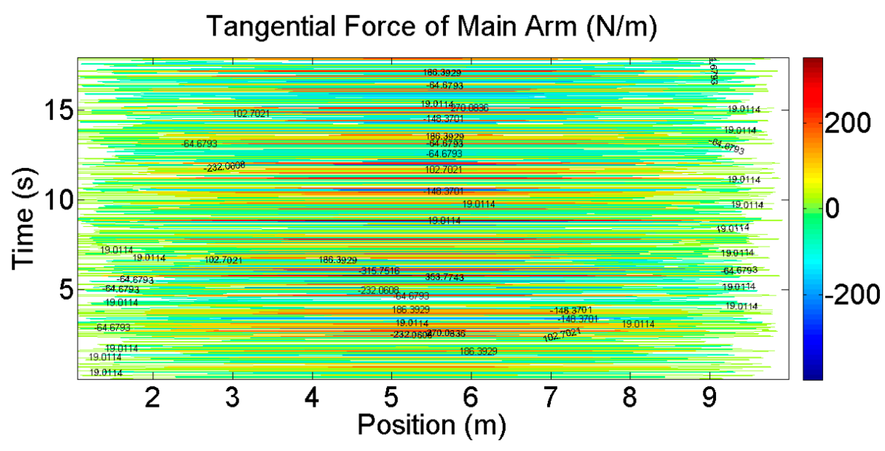
The main arms are in the horizontal plane and only a tangential force exists in Sec 4 (Figure 3d). The tangential force is obtained by integrating the wind pressure along the main arm and multiplying the depth of the main arm (1.2 m). The tangential force per unit length is shown in Figure 19. The length of the main arm is 10 m, and the origin is at the tower end. The largest force appears at the middle of the main arm, and the force becomes zero at both ends.
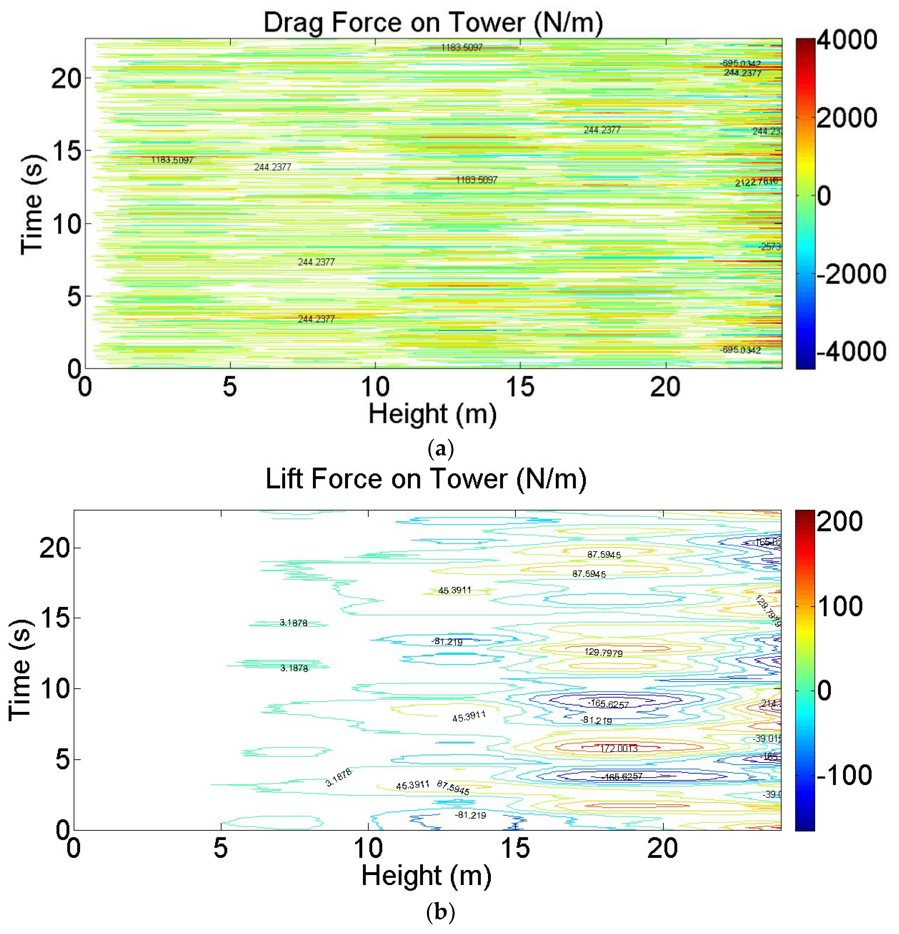
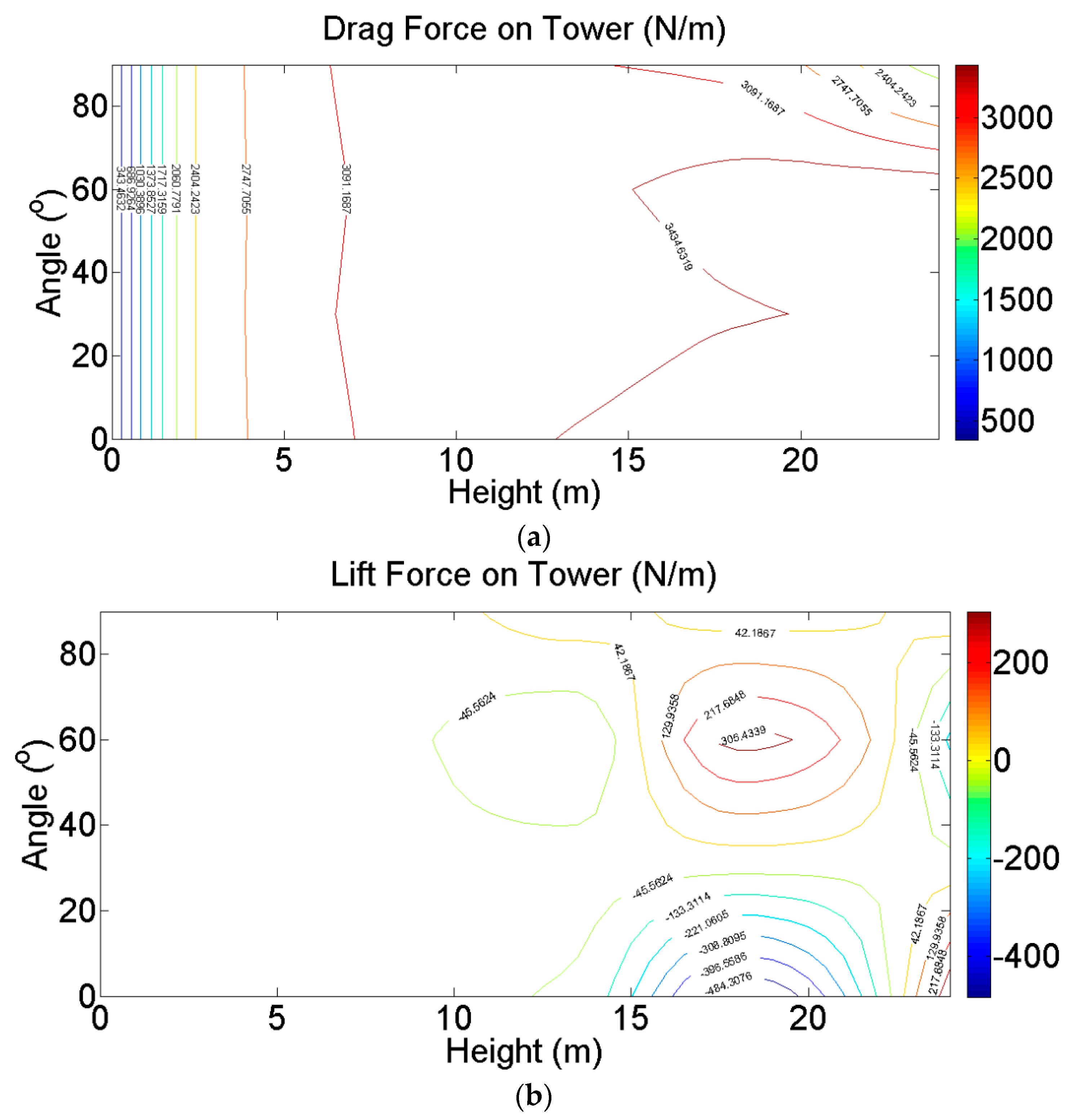
The drag and lift forces of the tower are obtained though integration of the wind pressure over the cross section, and are shown in Figure 20. The height of the tower is from 0 m to 24.28 m. The lift force in the range of 0–10.5 m is tiny because only the vortex shedding exists in the range. The lift force becomes much larger as the height is over 10.5 m, which is caused by the rotation of the blades and arms, the wake excitation, and the vortex shedding.
4.4. Wind Loads in the Extreme Wind Speed
The wind pressures on the blade and the aerodynamic forces on the entire VAWT under the extreme wind speed are also required to conduct the ultimate strength analysis that will be presented in the companion paper [46]. In the case, the VAWT is standing still without rotating. Thus, the wind loads vary with the change in the inflow wind direction in the simulation, and the inflow wind direction is represented by the azimuth angle (Figure 4).
Taking Sec 1 as the example, the wind pressures of the blade for four typical azimuth angles of 0°, 90°, 180°, and 270° are shown in Figure 21. When θ = 0°, the surfaces of the blade are under negative pressure, except the leading edge. The reason is that the wind speed is decreased at the leading edge, but accelerated over the surface, and finally re-attaches on the tailing edge. When θ = 90°, the wind pressure has a large negative value in the leading and trailing edges and the leeward surface. This result is because serious flow separations occur at the trailing edge under steady state when the azimuth angle is large, thereby resulting in the large negative wind pressure. The pressure distribution is quite different from that under the operational condition (Figure 15a). For θ = 180°, the wind flow comes to the trailing edge first and then goes through the surface up to the leading edge. In this case, the wind flow is stopped by the trailing edge and the positive pressure is thus induced in this area. The leading edge is the stagnation point, and the pressure at this point is nearly zero. When θ = 270°, the wind pressure distribution is similar to that when θ = 90°. Flow separation occurs at the leading edge and the trailing edge, which results in a large negative wind pressure at the two positions.
In the simulations, the near-wall y-plus values in Sec 1–Sec 9 are 1.5, 1.1, 1.5, 1.9, 1.6, 1.7, 1.7, 2.5, and 1.8, respectively. These values satisfy the near-wall requirement (y + < 5 for SST k-ω).
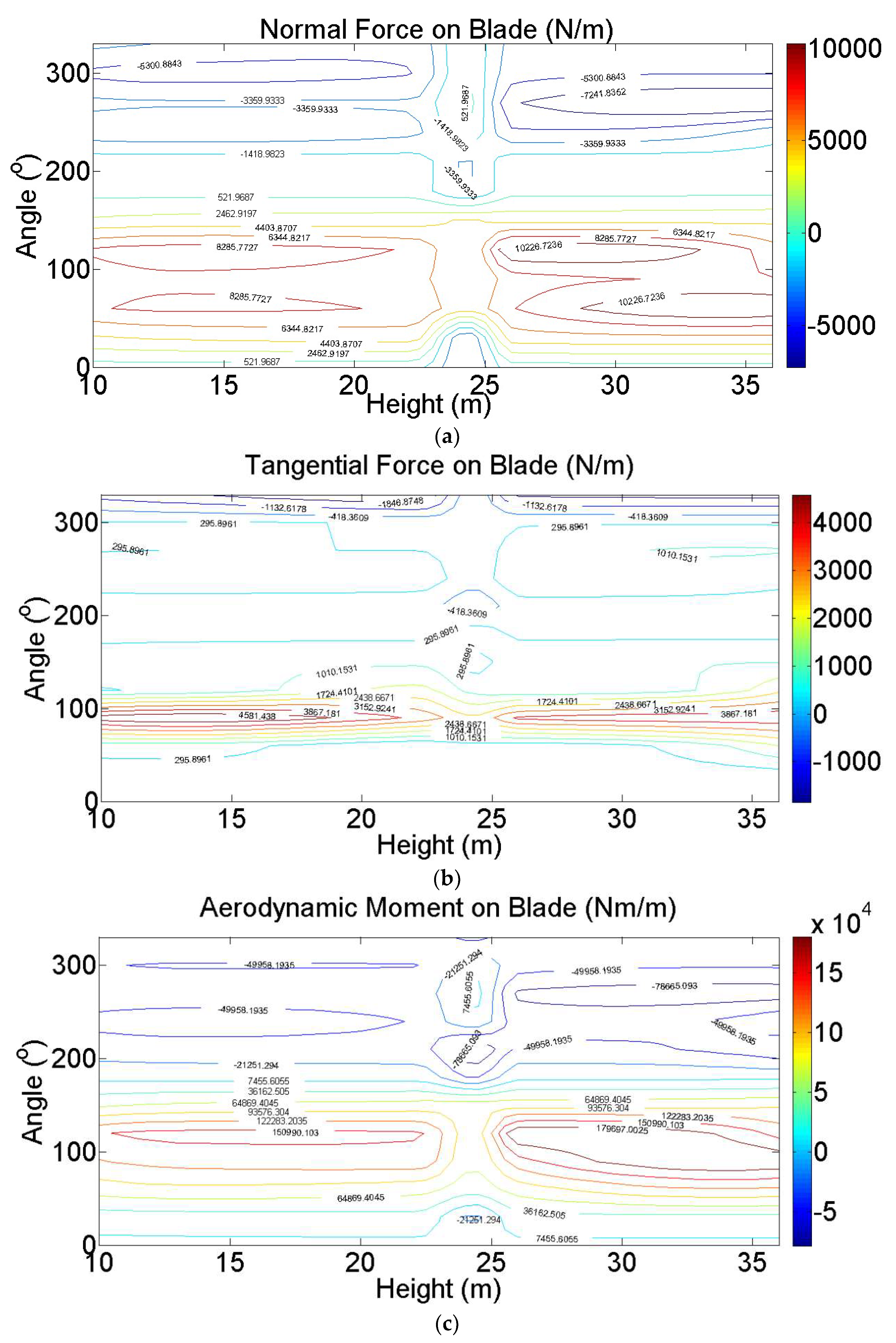
The VAWT with three straight blades is of threefold symmetry. Therefore, only the azimuth angles of 0°–120° are considered for the extreme wind speed case. Here, the azimuth angles of 0°, 30°, 60°, and 90° are simulated. The aerodynamic forces and moment on the VAWT at the azimuth angles of 0°, 30°, 60°, 90°, 120°, 150°, 180°, 210°, 240°, 270°, 300°, and 330° can then be obtained. The aerodynamic forces and moment at other azimuth angles are obtained through interpolation.
The normal and tangential forces and the moment per unit length of one blade are shown in Figure 22. The largest positive normal force on the blade appears at θ ∈ [60°, 120°], and the largest negative normal force on the same blade appears at θ ∈ [240°, 300°]. This observation is because the drag force is large in this range. In the upwind side (θ ∈ [60°, 120°]), the drag force results in a large positive normal force. In the downwind side (θ ∈ [240°, 300°]), the drag force results in a large negative normal force. The largest tangential force on the blade appears at θ = 90°. The aerodynamic moment on the blade has the largest value at θ = 90° and θ = 300°. Similar to the operating case, the aerodynamic forces in the higher section are generally larger than those in the lower section, which reflects the influence of the wind profile. The forces near Sec 4 are different from those in other sections because of the influence of the main arm.
The normal force, tangential force, and moment per unit length on the upper and lower arms are shown in Figure 23. For the normal force, two positive peaks occur in the upwind side (one at approximately θ = 60° and the other in the range of θ ∈ [120°, 150°]). Two negative peaks also appear in the downwind side (one at nearly θ = 210° and the other at around θ = 300°). For the tangential force, one positive peak (θ = 120°) and one negative peak (θ = 30°) appear in the upwind side. The aerodynamic moment reaches the largest positive value near θ = 120° and the largest negative value near θ = 120°.
The tangential force of the main arm is shown in Figure 24, which reaches the largest positive value at approximately θ = 150° and the largest negative value at nearly θ = 30°.
The aerodynamic forces of the tower, represented by the drag and the lift forces, are shown in Figure 25. Considering the symmetry, only the azimuth angle of θ ∈ [0°, 120°] is plotted. The drag force at the top of the tower is larger than the drag force at the bottom and approaches zero near the ground because of the mean wind profile. The lift force is relatively small because only the vortex shedding exists in this region, which is similar to the operating wind speed condition. For the height range above 10.5 m, the variation in the lift force with the azimuth angle is the result of the effects of the blades and lower arm.
5. Conclusions
The wind load simulation framework for the VAWT was established in this study by taking a prototype in Guangdong, China as an example. From the results of the present study, the following conclusions can be drawn.
- (1)
- The results from the 2.5D LES and the 2D SST simulations were compared. The two methods could obtain similar results for the cases of λ = 1 and λ = 3. In the case of λ = 1, the slight difference in the tangential force was because of the different predictions of flow separation. The 2D SST can be used as a proper model for determining the wind loads on VAWTs.
- (2)
- Using the 2D SST simulation, the wind pressures on blades and aerodynamic forces on the whole VAWT were obtained. The influences of turbulent inflow, tower, and arms on the aerodynamic forces on the blade were investigated. The tower of this large VAWT was far from the blades. Thus, the tower had a slight effect on the wind load of the blade and only caused a small reduction in the aerodynamic forces in the downwind side. The arms caused a considerable reduction in the tangential force and power coefficient.
- (3)
- Using the strip analysis method with a series of 2D SST k-ω simulations offers VAWT designers an engineering approach, which can obtain more detailed information of aerodynamics compared with DMST, while avoiding the intensive computational cost of 3D simulation.
- (4)
- Further quantifying the influence of support structure, such as arms and tower, and the accuracy of the proposed framework requires a high-fidelity 3D CFD simulation. More efforts should be directed toward this topic in the future.
Author Contributions
Conceptualization, Y.-L.X.; methodology, Y.-L.X. and J.L.; software, J.L.; validation, J.L., C.L., and Y.X.; formal analysis, J.L.; investigation, J.L.; resources, Y.-L.X.; data curation, J.L. and C.L.; writing—original draft preparation, J.L. and Y.-L.X.; writing—review and editing, Y.X.; visualization, J.L. and Y.X.; supervision, Y.-L.X.; project administration, Y.-L.X.; funding acquisition, Y.-L.X.
Funding
This research was funded by CII-HK/PolyU Research Fund (5-ZJE7).
Acknowledgments
The authors are grateful to Gordon YS Wu and Leo KK Leung of Hopewell Holdings Limited of Hong Kong for allowing the authors to use their innovative vertical axis wind turbine as a case study.
Conflicts of Interest
The authors declare no conflict of interest. The funder had no role in the design of the study; in the collection, analyses, or interpretation of data; in the writing of the manuscript; or in the decision to publish the results.
References
- Paraschivoiu, I. Wind Turbine Design—With Emphasis on Darrieus Concept; Presses Internationales Polytechnique: Montreal, QC, Canada, 2002. [Google Scholar]
- Almohammadi, K.M.; Ingham, D.B.; Ma, L.; Pourkashan, M. Computational fluid dynamics (CFD) mesh independency techniques for a straight blade vertical axis wind turbine. Energy 2013, 58, 483–493. [Google Scholar] [CrossRef]
- Balduzzi, F.; Bianchini, A.; Maleci, R.; Ferrara, G.; Ferrari, L. Critical issues in the CFD simulation of Darrieus wind turbines. Renew. Energy 2016, 85, 419–435. [Google Scholar] [CrossRef]
- Balduzzi, F.; Bianchini, A.; Ferrara, G.; Ferrari, L. Dimensionless numbers for the assessment of mesh and timestep requirements in CFD simulations of Darrieus wind turbines. Energy 2016, 97, 246–261. [Google Scholar] [CrossRef]
- Li, C.; Xiao, Y.; Xu, Y.; Peng, Y.; Hu, G.; Zhu, S. Optimization of blade pitch in h-rotor vertical axis wind turbines through computational fluid dynamics simulations. Appl. Energy 2018, 212, 1107–1125. [Google Scholar] [CrossRef]
- Meana-Fernández, A.; Oro, J.M.F.; Díaz, K.M.A.; Velarde-Suárez, S. Turbulence-Model Comparison for Aerodynamic-Performance Prediction of a Typical Vertical-Axis Wind-Turbine Airfoil. Energies 2019, 12, 488. [Google Scholar] [CrossRef]
- Lanzafame, R.; Mauro, S.; Messina, M. Wind turbine CFD modeling using a correlation-based transitional model. Renew. Energy 2013, 52, 31–39. [Google Scholar] [CrossRef]
- Li, C.; Zhu, S.; Xu, Y.L.; Xiao, Y. 2.5 D large eddy simulation of vertical axis wind turbine in consideration of high angle of attack flow. Renew. Energy 2013, 51, 317–330. [Google Scholar] [CrossRef]
- Ismail, M.F.; Vijayaraghavan, K. The effects of aerofoil profile modification on a vertical axis wind turbine performance. Energy 2015, 80, 20–31. [Google Scholar] [CrossRef]
- Amet, E.; Maître, T.; Pellone, C.; Achard, J.L. 2D numerical simulations of blade-vortex interaction in a darrieus turbine. J. Fluids Eng. 2009, 131, 111103. [Google Scholar] [CrossRef]
- Castelli, M.R.; Englaro, A.; Benini, E. The Darrieus wind turbine: Proposal for a new performance prediction model based on CFD. Energy 2011, 36, 4919–4934. [Google Scholar] [CrossRef]
- Danao, L.A.; Edwards, J.; Eboibi, O.; Howell, R. A numerical investigation into the influence of unsteady wind on the performance and aerodynamics of a vertical axis wind turbine. Appl. Energy 2014, 116, 111–124. [Google Scholar] [CrossRef] [Green Version]
- Mcintosh, S.C.; Babinsky, H.; Bertenyi, T. Unsteady Power Output of Vertical Axis Wind Turbines Operating within a Fluctuating Free-Stream. In Proceedings of the 46th AIAA Aerospace Sciences Meeting and Exhibit, Reno, Nevada, 7–10 January 2008. [Google Scholar]
- Scheurich, F.; Brown, R.E. Modelling the aerodynamics of vertical-axis wind turbines in unsteady wind conditions. Wind Energy 2013, 16, 91–107. [Google Scholar] [CrossRef]
- Ferreira, C.J.; Bijl, H.; van Bussel, G.; van Kuik, G. Simulating dynamic stall in a 2D VAWT: Modeling strategy, verification and validation with particle image velocimetry data. J. Phys. Conf. Ser. 2007, 75, 012–023. [Google Scholar] [CrossRef]
- Wang, S.; Ingham, D.B.; Ma, L.; Pourkashanian, M.; Tao, Z. Numerical investigations on dynamic stall of low Reynolds number flow around oscillating airfoils. Comput. Fluids 2010, 39, 1529–1541. [Google Scholar] [CrossRef]
- Rezaeiha, A.; Montazeri, H.; Blocken, B. Characterization of aerodynamic performance of vertical axis wind turbines: Impact of operational parameters. Energy Convers. Manag. 2018, 169, 45–77. [Google Scholar] [CrossRef]
- Hand, B.; Kelly, G.; Cashman, A. Numerical simulation of a vertical axis wind turbine airfoil experiencing dynamic stall at high Reynolds numbers. Comput. Fluids 2017, 149, 12–30. [Google Scholar] [CrossRef]
- Nini, M.; Motta, V.; Bindolino, G.; Guardone, A. Three-dimensional simulation of a complete vertical axis wind turbine using overlapping grids. J. Comput. Appl. Math. 2014, 270, 78–87. [Google Scholar] [CrossRef]
- Elkhoury, M.; Kiwata, T.; Aoun, E. Experimental and numerical investigation of a three-dimensional vertical-axis wind turbine with variable-pitch. J. Wind Eng. Ind. Aerod. 2015, 139, 111–123. [Google Scholar] [CrossRef]
- Omar, D.L.M.; Jhon, J.Q.; Santiago, L. RANS and Hybrid RANS-LES Simulations of an H-Type Darrieus Vertical Axis Water Turbine. Energies 2018, 11, 2348. [Google Scholar] [Green Version]
- Balduzzi, F.; Drofelnik, J.; Bianchini, A.; Ferrara, G.; Ferrari, L.; Campobasso, M.S. Darrieus Wind Turbine Blade Unsteady Aerodynamics: A Three-Dimensional Navier-Stokes CFD assessment. Energy 2017, 128, 550–563. [Google Scholar] [CrossRef]
- MacPhee, D.W.; Beyene, A. Fluid–structure interaction analysis of a morphing vertical axis wind turbine. J. Fluids Struct. 2016, 60, 143–159. [Google Scholar] [CrossRef]
- Yang, P.; Xiang, J.; Fang, F.; Pain, C.C. A fidelity fluid-structure interaction model for vertical axis tidal turbines in turbulence flows. Appl. Energy 2019, 236, 465–477. [Google Scholar] [CrossRef]
- Liu, K.; Yu, M.; Zhu, W. Enhancing wind energy harvesting performance of vertical axis wind turbines with a new hybrid design: A fluid-structure interaction study. Renew. Energy 2019, 140, 912–927. [Google Scholar] [CrossRef]
- Cachafeiro, H.; de Arevalo, L.; Vinuesa, R.; Goikoetxea, J.; Barriga, J. Impact of solar selective coating ageing on energy cost. Energy Procedia 2015, 69, 299–309. [Google Scholar] [CrossRef]
- Burton, T.; Sharpe, D.; Jenkins, N.; Bossanyi, E. Wind Energy Handbook; John Wiley & Sons: Hoboken, NJ, USA, 2001. [Google Scholar]
- Snel, H.; Schepers, J.G. Joint Investigation of Dynamic Inflow Effects and Implementation of an Engineering Method; ECN: Sint Maartensvlotbrug, The Netherlands, 1995. [Google Scholar]
- Wendler, J.; Marten, D.; Pechlivanoglou, G.; Nayeri, C.; Paschereit, C. An unsteady aerodynamics model for lifting line free vortex wake simulations of HAWT and VAWT in QBlade. In Proceedings of the ASME Turbo Expo 2016: Turbomachinery Technical Conference and Exposition, Seoul, Korea, 13–17 June 2016. [Google Scholar]
- Lei, H.; Zhou, D.; Bao, Y.; Chen, C.; Ma, N.; Han, Z. Numerical simulations of the unsteady aerodynamics of a floating vertical axis wind turbine in surge motion. Energy 2017, 127, 1–17. [Google Scholar] [CrossRef]
- Wekesa, D.W.; Wang, C.; Wei, Y.; Kamau, J.N.; Danao, L.A.M. A numerical analysis of unsteady inflow wind for site specific vertical axis wind turbine: A case study for Marsabit and Garissa in Kenya. Renew. Energy 2015, 76, 648–661. [Google Scholar] [CrossRef]
- Danao, L.A.; Eboibi, O.; Howell, R. An experimental investigation into the influence of unsteady wind on the performance of a vertical axis wind turbine. Appl. Energy 2013, 107, 403–411. [Google Scholar] [CrossRef]
- Mcintosh, S.C.; Babinsky, H.; Bertenyi, T. Optimizing the Energy Output of Vertical Axis Wind Turbines for Fluctuating Wind Conditions. In Proceedings of the 45th AIAA Aerospace Sciences Meeting and Exhibit, Reno, Nevada, 8–11 January 2007. [Google Scholar]
- Simiu, E.; Scanlan, R.H. Wind Effects on Structures: An Introduction to Wind Engineering; John Wiley: New York, NY, USA, 1986. [Google Scholar]
- Xu, Y.L. Wind Effects on Cable-Supported Bridges; John Wiley & Sons: Hoboken, NJ, USA, 2013. [Google Scholar]
- International Electrotechnical Commission. IEC 61400-1: Wind Turbines Part 1: Design Requirements, 3rd ed.; IEC: Geneva, Switzerland, 2015. [Google Scholar]
- Vinuesa, R.; Nagib, H. Enhancing the accuracy of measurement techniques in high Reynolds number turbulent boundary layers for more representative comparison to their canonical representations. Eur. J. Mech. B Fluid. 2016, 55, 300–312. [Google Scholar] [CrossRef]
- Shinozuka, M.; Jan, C.M. Digital simulation of random processes and its applications. J. Sound Vib. 1972, 25, 111–128. [Google Scholar] [CrossRef]
- Chen, X.; Kareem, A. Equivalent static wind loads on buildings: New model. J. Struct. Eng. ASCE 2004, 130, 1425–1435. [Google Scholar] [CrossRef]
- Vinuesa, R.; Hosseini, S.; Hanifi, A.; Henningson, D.; Schlatter, P. Pressure-gradient turbulent boundary layers developing around a wing section. Flow Turbul. Combust. 2017, 99, 613–641. [Google Scholar] [CrossRef] [PubMed]
- Chattot, J.; Hafez, M. Wind Turbine and Propeller Aerodynamics—Analysis and Design. In Theoretical and Applied Aerodynamics; Springer: Berlin, Germany, 2015; pp. 327–372. [Google Scholar]
- Davenport, A.G. The use of taut-strip models in the prediction of the response of long span bridges to turbulent wind. In Proceedings of the IUTAM/IAHR Symposium on Flow-Induced Structural Vibrations, Karlsruhe, Germany, 14–16 August 1972. [Google Scholar]
- Menter, F.R.; Kuntz, M.; Langtry, R. Ten years of industrial experience with the SST turbulence model. In Turbulence, Heat and Mass Transfer 4; Begell House, Inc.: New York, NY, USA, 2003. [Google Scholar]
- Barnes, W.; McCormick, W. Aerodynamics, Aeronautics, and Flight Mechanics (Volume 2); Wiley: New York, NY, USA, 1995. [Google Scholar]
- ANSYS. 12.0 User’s Guide; Ansys Inc.: Canonsburg, PA, USA, 2009. [Google Scholar]
- Lin, J.H.; Xu, Y.L.; Xia, Y. Structural Analysis of Large-scale Vertical Axis Wind Turbines, Part II: Fatigue and Ultimate Strength Analyses. Energies 2019. accepted for publication. [Google Scholar]
Figure 1.
Prototype of a straight-bladed vertical-axis wind turbine (VAWT).

Figure 2.
Wind field and structural configuration of a VAWT.

Figure 3.
Plan layout of the selected sections: (a) Sec 1; (b) Sec 2; (c) Sec 3; (d) Sec 4; (e) Sec 5; (f) Sec 6; (g) Sec 7; (h) Sec 8 and Sec 9.
Figure 3.
Plan layout of the selected sections: (a) Sec 1; (b) Sec 2; (c) Sec 3; (d) Sec 4; (e) Sec 5; (f) Sec 6; (g) Sec 7; (h) Sec 8 and Sec 9.

Figure 4.
Scheme of geometry and boundaries for wind load simulation.

Figure 5.
Mesh grids of the flow field: (a) entire flow field; (b) zones 2 and 3; (c) around a blade; (d) zone 3.
Figure 5.
Mesh grids of the flow field: (a) entire flow field; (b) zones 2 and 3; (c) around a blade; (d) zone 3.

Figure 6.
Mesh and time-step sensitivity study: (a) mesh sensitivity study; (b) time-step sensitivity study.
Figure 6.
Mesh and time-step sensitivity study: (a) mesh sensitivity study; (b) time-step sensitivity study.

Figure 7.
Cross section of a NACA0018 blade.

Figure 8.
Wind pressure time histories (λ = 1): (a) points A and B; (b) points C and D. LES—large eddy simulation; SST—shear stress transport.
Figure 8.
Wind pressure time histories (λ = 1): (a) points A and B; (b) points C and D. LES—large eddy simulation; SST—shear stress transport.

Figure 9.
Wind pressure time histories (λ = 3): (a) points A and B; (b) points C and D.

Figure 10.
Wind pressure distributions of the blade (λ = 1): (a) θ = 30°; (b) θ = 50°; (c) θ = 70°.

Figure 11.
Wind pressure distributions of the blade (λ = 3): (a) θ = 60°; (b) θ = 105°; (c) θ = 130°.
Figure 11.
Wind pressure distributions of the blade (λ = 3): (a) θ = 60°; (b) θ = 105°; (c) θ = 130°.

Figure 12.
Comparisons of normal force coefficient Cn and tangential force coefficient Ct: (a) λ = 1; (b) λ = 3.
Figure 12.
Comparisons of normal force coefficient Cn and tangential force coefficient Ct: (a) λ = 1; (b) λ = 3.

Figure 13.
Wind speed time history of Sec 4.

Figure 14.
Time-varying wind pressures on Sec 1: (a) points A and B; (b) points C and D.

Figure 15.
Wind pressures of blade in Sec 1–Sec 7 (θ = π/2): (a) Sec 1; (b) Sec 2; (c) Sec 3; (d) Sec 4; (e) Sec 5; (f) Sec 6; (g) Sec 7.
Figure 15.
Wind pressures of blade in Sec 1–Sec 7 (θ = π/2): (a) Sec 1; (b) Sec 2; (c) Sec 3; (d) Sec 4; (e) Sec 5; (f) Sec 6; (g) Sec 7.


Figure 16.
Variation in wind pressures along the height at t = 18.70 s (θ = π/2).

Figure 17.
Aerodynamic forces on a blade: (a) normal force; (b) tangential force; (c) moment.

Figure 18.
Aerodynamic forces and moment per unit length of lower and upper arms: (a) normal force on a lower arm; (b) normal force on an upper arm; (c) tangential force on a lower arm; (d) tangential force on an upper arm; (e) moment on a lower arm; (f) moment on an upper arm.
Figure 18.
Aerodynamic forces and moment per unit length of lower and upper arms: (a) normal force on a lower arm; (b) normal force on an upper arm; (c) tangential force on a lower arm; (d) tangential force on an upper arm; (e) moment on a lower arm; (f) moment on an upper arm.


Figure 19.
Tangential force on a main arm.

Figure 20.
Aerodynamic forces per unit length on the tower: (a) drag force; (b) lift force.

Figure 21.
Wind pressures on the blade for Sec 1 under the extreme wind speed: (a) θ = 0°; (b) θ = 90°; (c) θ = 180°; (d) θ = 270°.
Figure 21.
Wind pressures on the blade for Sec 1 under the extreme wind speed: (a) θ = 0°; (b) θ = 90°; (c) θ = 180°; (d) θ = 270°.


Figure 22.
Aerodynamic forces and moment per unit length on the blade under the extreme wind condition: (a) Normal force; (b) Tangential force; (c) Moment.
Figure 22.
Aerodynamic forces and moment per unit length on the blade under the extreme wind condition: (a) Normal force; (b) Tangential force; (c) Moment.

Figure 23.
Aerodynamic forces per unit length on the upper and lower arms: (a) normal force on the upper arm; (b) tangential force on the upper arm; (c) moment on the upper arm; (d) normal force on the lower arm; (e) tangential force on the lower arm; (f) moment on the lower arm.
Figure 23.
Aerodynamic forces per unit length on the upper and lower arms: (a) normal force on the upper arm; (b) tangential force on the upper arm; (c) moment on the upper arm; (d) normal force on the lower arm; (e) tangential force on the lower arm; (f) moment on the lower arm.


Figure 24.
Tangential force per unit length on the main arm.

Figure 25.
Drag and lift forces on the tower: (a) drag force; (b) lift force.


Table 1.
Elevations of the selected sections.
| Section | Sec 1 | Sec 2 | Sec 3 | Sec 4 | Sec 5 | Sec 6 | Sec 7 | Sec 8 | Sec 9 |
|---|---|---|---|---|---|---|---|---|---|
| Elevation above ground (m) | 34.0 | 29.7 | 26.1 | 24.3 | 22.2 | 18.1 | 13.3 | 7.9 | 2.6 |
Table 2.
Number of grids of nine sections.
| Section | Sec 1 | Sec 2 | Sec 3 | Sec 4 | Sec 5 | Sec 6 | Sec 7 | Sec 8 | Sec 9 |
|---|---|---|---|---|---|---|---|---|---|
| Grid Number | 217,432 | 299,032 | 279,832 | 238,232 | 277,832 | 277,832 | 231,032 | 88,432 | 88,432 |
© 2019 by the authors. Licensee MDPI, Basel, Switzerland. This article is an open access article distributed under the terms and conditions of the Creative Commons Attribution (CC BY) license (http://creativecommons.org/licenses/by/4.0/).
Share and Cite
MDPI and ACS Style
Lin, J.; Xu, Y.-L.; Xia, Y.; Li, C. Structural Analysis of Large-Scale Vertical-Axis Wind Turbines, Part I: Wind Load Simulation. Energies 2019, 12, 2573. https://doi.org/10.3390/en12132573
AMA Style
Lin J, Xu Y-L, Xia Y, Li C. Structural Analysis of Large-Scale Vertical-Axis Wind Turbines, Part I: Wind Load Simulation. Energies. 2019; 12(13):2573. https://doi.org/10.3390/en12132573
Chicago/Turabian StyleLin, Jinghua, You-Lin Xu, Yong Xia, and Chao Li. 2019. "Structural Analysis of Large-Scale Vertical-Axis Wind Turbines, Part I: Wind Load Simulation" Energies 12, no. 13: 2573. https://doi.org/10.3390/en12132573
Note that from the first issue of 2016, this journal uses article numbers instead of page numbers. See further details here.