Testing and Validation of Adaptive Impedance Matching System for Broadband Antenna

1
Department of Engineering Technology and Industrial Distribution, Texas A&M University, College Station, TX 77843, USA
2
Department of Electrical and Computer Engineering, University of Florida, Gainesville, FL 32611, USA
3
Department of Electrical and Computer Engineering, University of Arizona, Tucson, AZ 85721, USA
*
Author to whom correspondence should be addressed.
Electronics 2019, 8(9), 1055; https://doi.org/10.3390/electronics8091055
Submission received: 1 August 2019
/
Revised: 8 September 2019
/
Accepted: 17 September 2019
/
Published: 19 September 2019
(This article belongs to the Section Microwave and Wireless Communications)
Abstract
:Broad RF impedance matching is challenging; however, the need for broadband matching is found frequently in modern RF and wireless systems with multiple wireless standards. Moreover, in 5G technology, multiple frequency bands are used, and these systems typically employ a broadband antenna or multiple antennas. Antenna impedances vary from design targets for many reasons including manufacturing process variations or antenna environment changes. An adaptive impedance matching system (AIMS) for testing and validation is introduced, and its implementation is shown in this paper. The AIMS can control impedance matching tuner settings to provide an arbitrary impedance frequency-varying load that meets user-defined conditions. This AIMS provides a testing and validation system for broadband antennas that can be characterized by various settings of the impedance matching tuner. As a device under test (DUT), a three-stub reconfigurable filter was used as the impedance matching tuner on a RT/Duroid 6010 RF board. It was integrated with a control circuit board. This AIMS implementation also included an antenna impedance tuner that can vary the distance between the antenna and the ground plane. This model represents practical antenna impedance variations. The AIMS controls a network analyzer and the impendence matching tuner. The adaptive control program on a PC was developed to perform an effective two-pass tuning strategy. This article presents the successful automated tuned results and their numerical evaluations of three cases that were generated by the antenna impedance tuner.
1. Introduction
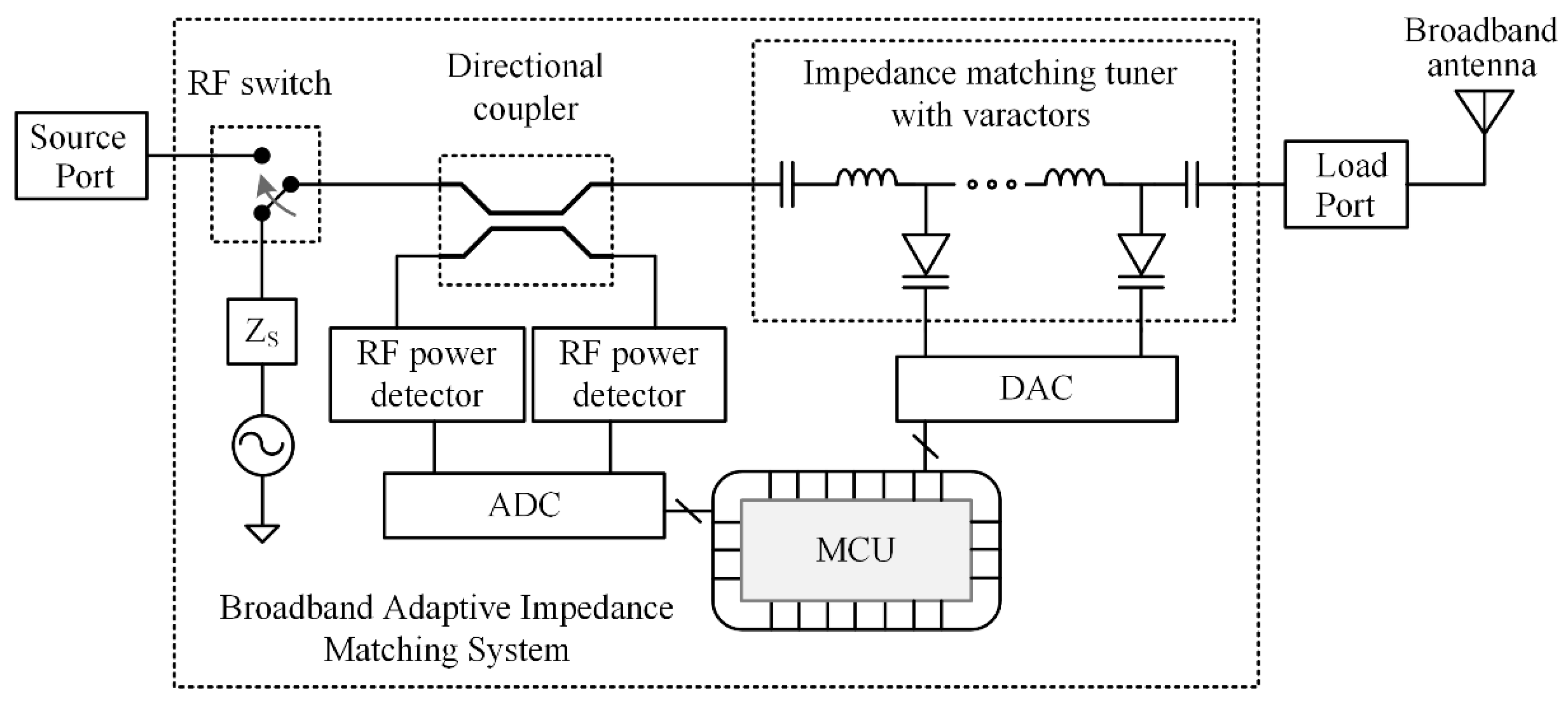
Modern wireless devices include multiple wireless transceivers or reconfigurable wireless transceiver components in order to meet the needs of various wireless standards. Wireless components may share a broadband antenna or have multiple antennas. Multiple-input and multiple-output (MIMO) is an example of the use of multipath propagation [1,2,3,4,5]. The 5G wireless data network standard adopts a massive MIMO system [6]. RF impedance matching for these broadband antenna impedances is often performed by an RF engineer. This manual broadband RF impedance matching is challenging because a good matching result at one frequency might result in poor matching at other frequencies [7]. Although RF circuit parameters can be obtained by this manual engineering effort or by computer simulation, these pre-determined circuit parameters for RF impedance matching may still need to be modified after the RF system is fabricated. This need for circuit modification may result from systematic or arbitrary variations of parasitics that are easily introduced into the RF network through manufacturing processes. Although the broadband antenna may be acceptable after fabrication, the antenna RF impedance matching may still need to be modified for many reasons such as antenna environmental changes or a close proximity to conductive objects such as humans or animals [8]. In order to provide an adaptive broadband matching between two RF ports, an adaptive broadband impedance matching system (AIMS) is introduced in this paper. A generalized conceptual block diagram of the AIMS is shown in Figure 1. If a broadband antenna is connected to a load port, the AIMS can tune and provide RF impedances that meet predefined conditions. A similar concept has been used as automatic tuning architectures in radar and wireless communication systems [9,10,11,12,13,14,15,16,17,18]. The testing and validation system of the broadband adaptive impedance matching applications is implemented and described in detail here. These results can be applied in a wide range of broadband antenna RF impedance matching tests and broadband antenna development tasks. The AIMS includes a broadband impedance matching tuner, which provides adaptive tuning functions. Stub-based reconfigurable filters can be employed as this impedance matching network [19,20]. In the implementation in this paper, one of the author’s stub-based reconfigurable filter was adopted as a device under test (DUT) [14]. The tuning method involves the control of varactor voltages that can change frequency characteristics of the matching tuner. The voltages of the varactors can be pre-determined by simulations. However, these pre-determined varactor voltages may easily provide unsatisfactory results and may need to be modified due to unwanted manufacturing process variations. This AIMS is capable of providing adaptive impedance matching and searching for optimum varactor voltages in real-time to meet the user-defined matching conditions. The AIMS can compensate for both random and systematic inaccuracies of RF impedance introduced at the RF ports. An early result of this research was introduced in the first author’s Ph.D. dissertation. In this paper, further details of the test system of the AIMS are presented, as well as the measurement and demonstration with the numerical evaluations.
2. Adaptive Broadband Impedance Matching System
This AIMS enables broadband RF impedance matching from varying load impedances to a source impedance. As shown in Figure 1, the tuning method involves changing the capacitance values of the matching filter. The implementation of this method can be achieved by the use of varactors, which can change their capacitances by varying bias voltages. In order to measure the reflection ratio, a directional coupler can be utilized [21,22]. In addition, a local variable oscillator and an RF switch are used to launch test signals for the reflection tests. For the detection of the power levels of the waves, RF power detectors can be utilized [23,24]. The output of these power detectors can be read by an analog-to-digital converter (ADC) module. The converted digital signals of the ADC can be processed by a microcontroller (MCU). Then, the MCU determines the control voltages to be applied to the varactors using a digital-to-analog converter (DAC).
2.1. Hardware Implementation of the AIMS for Testing and Validation
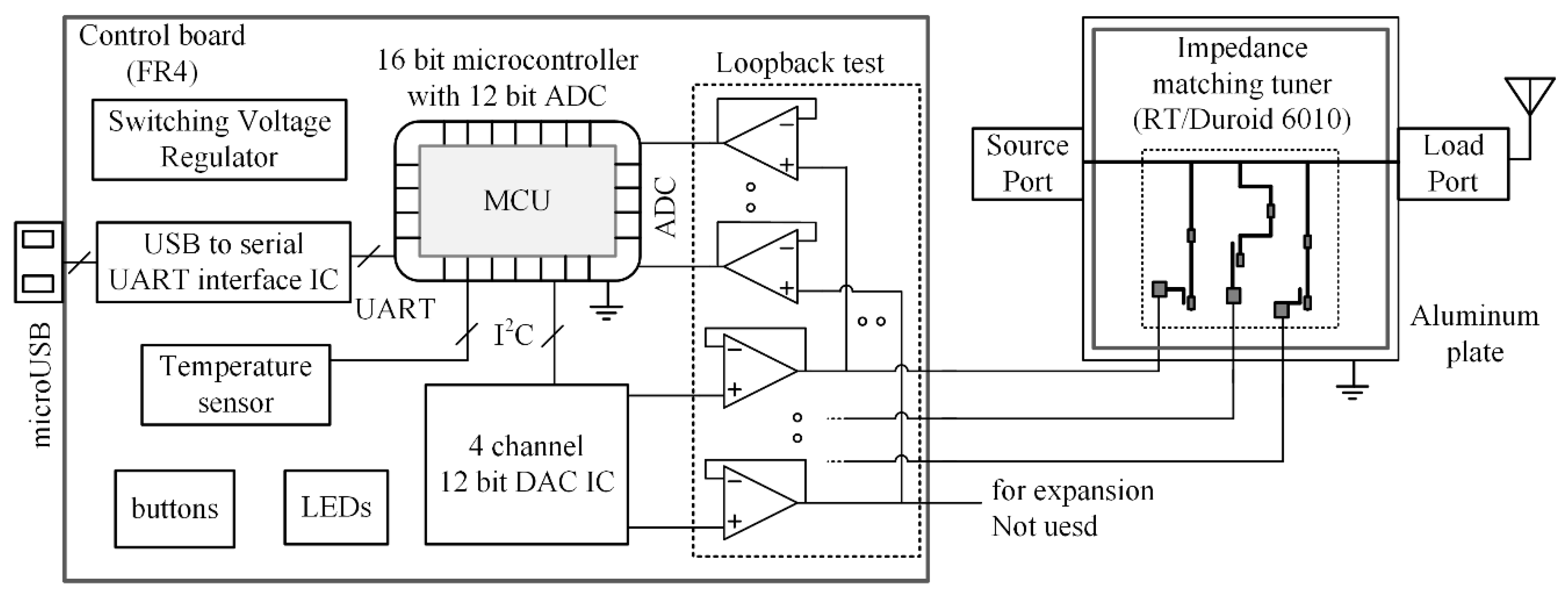
A functional block diagram of the implemented AIMS is shown in Figure 2. A control circuit board was built and assembled with the impedance matching tuner on an aluminum plate. The printed circuit board (PCB) material for the control board is FR-4, which is a common material for PCBs. The PCB material for the impedance matching tuner is a RF board material, RT/Duroid 6010. Both of these PCBs were mounted on an aluminum plate, which is a chassis ground. There are MCU, ADC, and DAC components on the control board. A low-power Texas Instrument (TI), MSP430, is adopted as the MCU. Active and sleep modes are used to save power. A 12-bit DAC from Microchip Technology is used to provide three stable control voltages. A loop-back test circuit monitors the status of the control voltages in the test environment and is connected to the MCU 12-bit ADCs. Additionally, the control board includes a USB interface IC to communicate with other instruments or a control PC. The USB interface IC and MCU on the same board communicate with each other through a universal asynchronous receiver-transmitter (UART). The control board includes an external digital temperature sensor to monitor the test and measurement environment, as well as LEDs and buttons to provide a user interface to control and check the status of the board.
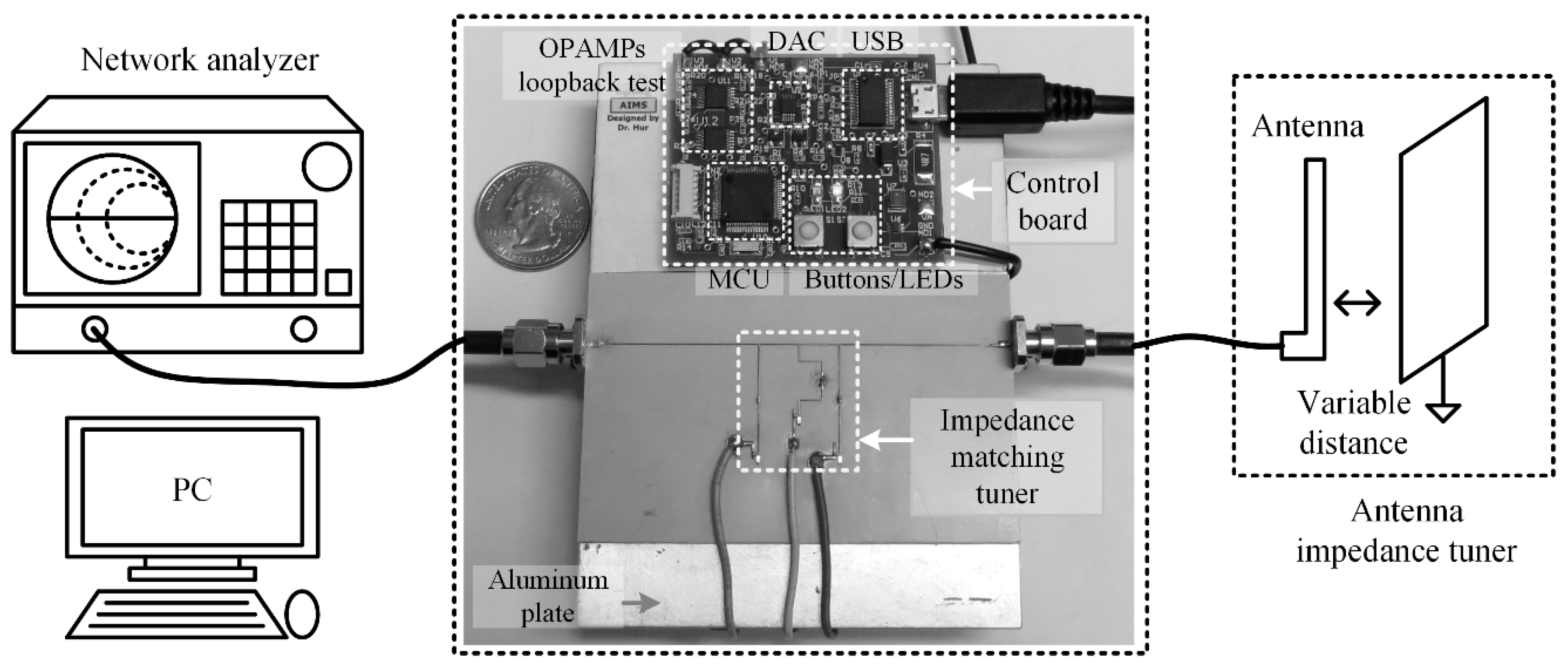
As an impedance tuner, the microstrip reconfigurable filter with three stubs is employed, as shown on the right side of Figure 3. This reconfigurable filter is part of the software-defined match control circuit. It has three stubs with a microstrip-loaded line structure on a 0.254-mm thick RT/Duroid 6010. This impedance matching tuner was designed and previously verified for multiple frequency bands. In the prior work, the tuning voltages were provided by external power supply circuits. These voltages were manually adjusted within the range of pre-determined values. In the current work, varactor power is integrated with the control circuit board and the tuning is automated by controlling three varactor voltage levels automatically as a closed loop test system. The size of the impedance matching tuner is 19 mm × 13 mm. The overall size of the integrated unit is 85 mm × 53 mm. A U.S. 25 cent piece coin on the left side of the PCB in Figure 3 is included for size comparison. A network analyzer connected to the source port provides the directional coupler and power detector components.
On the right side of Figure 3, a block diagram of the antenna impedance tuner is shown. The purpose of this antenna tuner is to emulate physical and real impedance variations similar to the placement of the antenna next to an arbitrary metal plate or a human. This is accomplished by modifying the distance between the antenna and an external metal plate. This proposed method can emulate realistic impairments to demonstrate the AIMS’ ability to effectively solve the RF impedance matching variation and optimization problem, emulating real antenna variation cases.
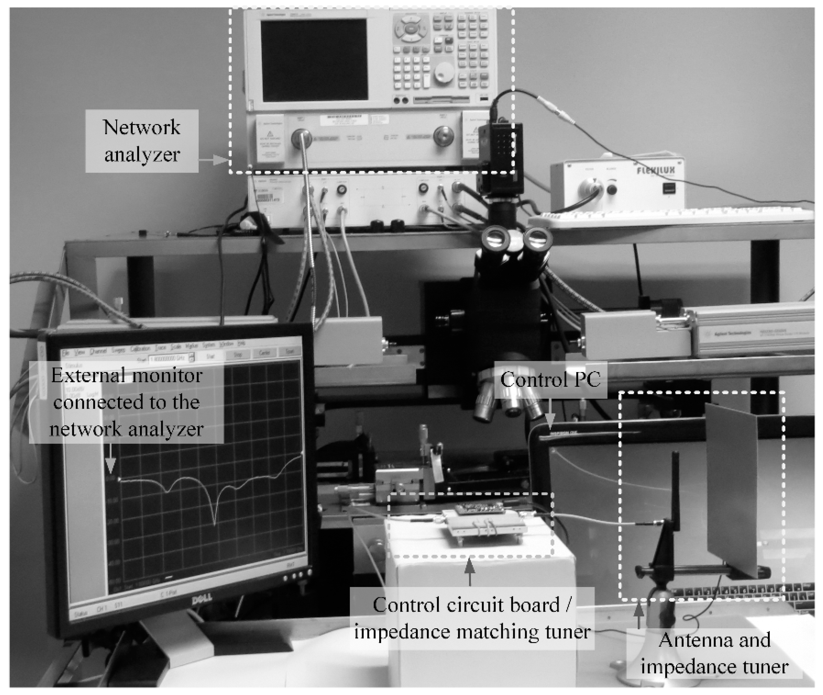
A photo of the testing and validation system of the AIMS is shown in Figure 4. The implementation of the antenna impedance tuner is shown on the right side. An antenna and a metal plate are placed on the mini vise, and the gap between them can be adjusted to demonstrate adaptive matching. This antenna impedance tuner was designed to provide a maximum gap of around 70 mm. In the center, the integrated board unit with the impedance tuner board and control circuit board is shown. The antenna is connected to the right side RF port, and the network analyzer is connected to the left side RF port. A network analyzer and a control PC are shown, and they can measure reflection coefficients and perform the custom search and control program by communicating with instruments and the control board. The control program will be described in the next section.
2.2. Software Implementation of the AIMS
The custom search and control program was developed using the MATLAB script language. In order to control instrumentation through Virtual Instrument Standard Architecture (VISA), an instrumentation control box may need to be installed on top of the standard MATLAB tool boxes. The MATLAB software communicates with the control board to send DAC levels and to receive the loopback voltage readings through ADCs to ensure the working condition of the DACs and the measurements. MATLAB also receives external digital temperature sensor data and time stamps. The software also commutates with a network analyzer to receive the reflection coefficients. The control program determines matching conditions based on user-defined reflection coefficient patterns and conditions. There are two types of conditions applied in this paper. One of them is “Uniform −10 dB” and the other one is non-uniform “−12 and −10 dB.” First, the uniform condition determines the pass or fail based on simply −10 dB reflection coefficients within the bandwidth of interest. In this paper, the frequency band is defined from 2 to 2.6 GHz, which may include the lower frequency band of MIMO Wireless Local Area Network (WLAN) applications. Another test condition is a non-uniform frequency response condition, which determines the test pass or fail based on more constraints of −12 dB reflection coefficients from 2.25 to 2.35 GHz, and −10 dB reflection coefficients in other frequencies within the bandwidth of interest. Having stricter conditions on the frequency band response was chosen as a difficult example. In the United States, the frequency band from 2.3 to 2.31 GHz is used by an amateur radio, and a satellite-based digital audio radio service (DARS) uses the bandwidth from 2.31 to 2.36 GHz. This non-uniform approach allows the control program to search for better matching conditions on a certain band of interest.
This custom search and control program finds an optimum bias control setting using a two-pass strategy. For the first pass, a coarse bias search is performed by applying three states of high, middle, and low voltages using the full control voltage range. There are three varactors to be controlled; therefore, for the coarse search, the program executes the maximum 81 cycles, which was determined by the third power of 3. For the second pass, a fine search is performed, which may result in better results. The general search methods for both the first and second passes are similar. However, for the second pass, the search uses a smaller voltage range that is within the optimal control voltages found in the first pass. For the fine search, the program also executes the maximum 81 cycles. However, in order to reduce the number of cycles, the fine search loop stops once it meets certain conditions. If needed, additional searching iterations, such as a 3rd pass, can be performed to obtain more precise results. However, in this configuration, the two-pass strategy is found to be reasonable due to the trade-off between the number of cycles and quality of the results.
The search and control program can be implemented in other software platforms, for example, LabVIEW. LabVIEW provides a graphical programming environment with GPIB (General Purpose Interface Bus) interfacing software. For an open-source and free software package, Python also provides a good programming and development environment. An open-source GPIB interface software that controls those instruments is available in Python as well.
3. Measurements and Automated Tuning Demonstrations
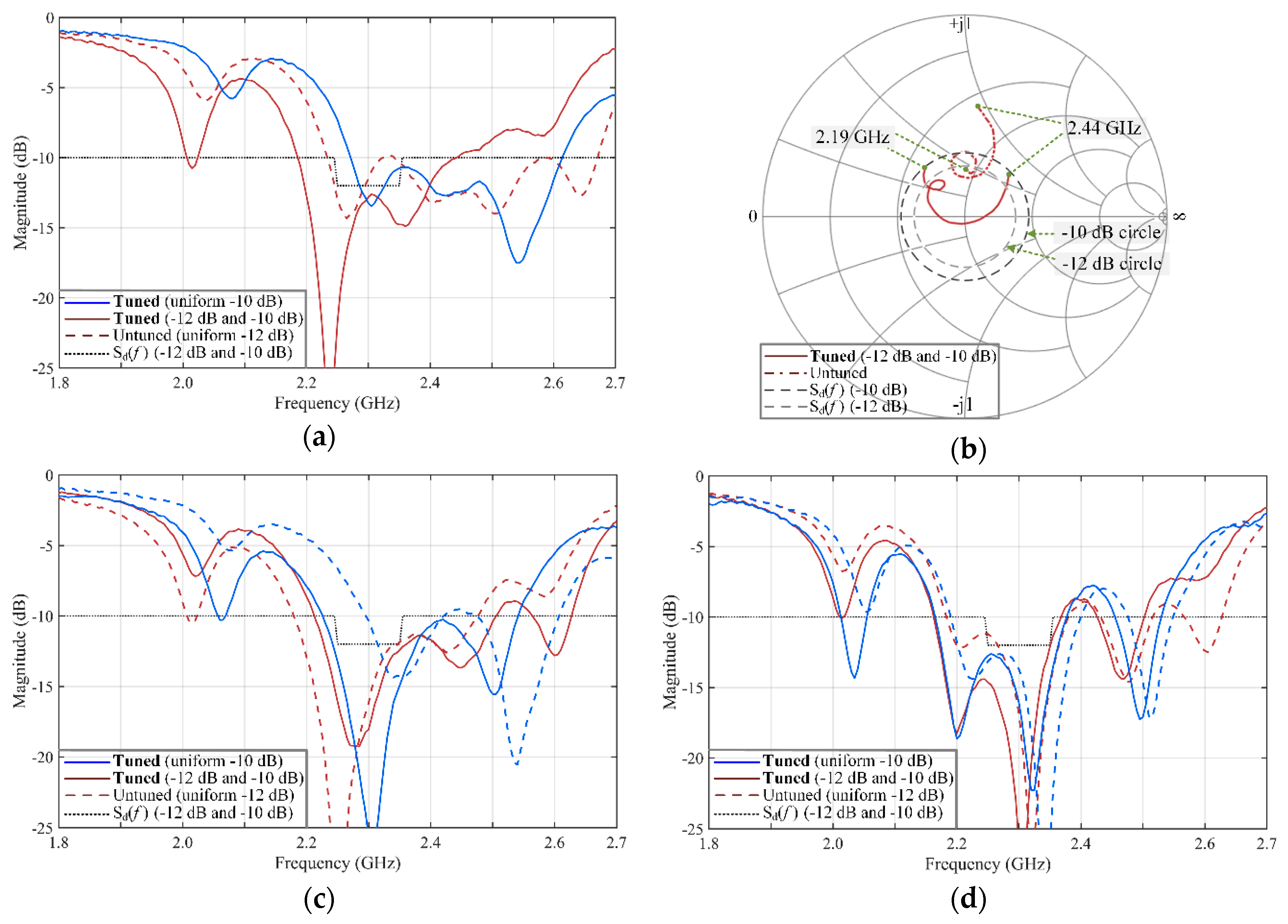
The antenna impedance tuner was initially configured to have a gap of 60 mm between the antenna and the metal plate. The varactor control voltage settings were set to their initial values of −1.5 V. Next, automatic tuning was performed to generate a new set of voltage settings and achieve a suitable broadband impedance match. With the varactor control voltages set to their optimum values found for the 60 mm gap, the physical gap between the antenna and metal plate was set to 40 mm, which resulted in a poor impedance match. Automatic tuning was then performed to determine the varactor voltages for a good impedance match for this gap setting. With the varactor control voltages set to their optimum values found for the 40 mm gap, the physical gap between the antenna and the metal plate was set to 20 mm. Again, automatic tuning was performed to determine the varactor voltages for a good impedance match for this gap setting. This sequential measurement and demonstration set of testing was carried out, and its results are shown in Figure 5.
3.1. Automated Antenna Matching Demonstrations for Varying Antenna Impedance Cases
The measured antenna impedances at 2.1, 2.3, and 2.5 GHz were included. For the initial 60 mm antenna/plate gap, the measured antenna impedances are 48.5 + j57.8, 40.2 − j19.9, and 43.8 − j7.4 Ω at 2.1, 2.3, and 2.5 GHz, respectively. The reflection magnitudes in decibels are −5.9, −12.4, and −19.7 dB at 2.1, 2.3, and 2.5 GHz, respectively. These values indicate the frequency-dependent nature of the input impedance and reflection coefficient. Figure 5a shows the “untuned” and “tuned” results. “Untuned” indicates the reflection coefficients before automated tuning. For tuned results, there are two matching conditions indicated by the legends “uniform” and “−12 and −10 dB.” These are the decision criteria described in the previous section. Figure 5b shows the Smith chart of untuned and tuned results of the gap of 60 mm for the uniform and the non-uniform case. The return losses of tuned results were less than −10 dB from 2.19 to 2.44 GHz, which was the frequency range of choice. Untuned results are shown as dash-dotted lines, which were not completely within the −10 dB constant circle, and not acceptable in the frequency range of choice.
For the 40 mm gap case of Figure 5c, the measured antenna impedances are 55.7 + j47.0, 53.2 − j20.9, and 36.0 − j1.9 at 2.1, 2.3, and 2.5 GHz, respectively. The magnitudes in decibels are −7.8, −14.0, and −15.7 dB at 2.1, 2.3, and 2.5 GHz, respectively. The optimum varactor control voltage sets for uniform and non-uniform cases were different. Hence, there were two different untuned results of these two cases, which are drawn as dashed lines. Blue lines show uniform cases and brown lines show non-uniform cases. Dashed lines show untuned results and solid lines show tuned results.
For the 20 mm gap case of Figure 5d, the measured antenna impedances are 78.8 + j45.5, 56.5 − j2.6, and 31.3 − j13.4 Ω at 2.1, 2.3, and 2.5 GHz, respectively. The magnitudes in decibels are −8.1, −23.7, and −11.1 dB at 2.1, 2.3, and 2.5 GHz, respectively. The tuned results are shown. After tuning, the results were shown to meet the return loss conditions. As the spacing between the metal plate and the antenna gets smaller from 60 to 20 mm, the circuit becomes less flexible in tuning. The details of the numerical evaluations used in measurements and demonstrations are followed in the next section.
3.2. Decision Method and Numerical Evaluations
The desired (condition) reflection coefficient determines if the measured reflection coefficient passes or fails, and this information can be used to calculate the effective bandwidth. The ratio of the two reflection coefficients is a decision reflection coefficient, and it can be defined as
Determining if the measured reflection coefficient passes or fails using the decision reflection coefficient can be performed by checking if the magnitude of the decision reflection coefficient is higher or lower than 1 in magnitude, which is 0 dB.
If and are the highest and lowest test frequencies, respectively, and they are equally divided into N test frequency points, then, new discrete test frequencies can be defined as
An average of the decision reflection coefficient’s magnitudes can be determined by
Similarly, a standard deviation of the decision reflection coefficient’s magnitudes can be obtained by
Table 1 shows the numerical evaluations for the pre- and post-tuned measurements of the 60, 40, and 20 mm cases, which are shown in Figure 5a,c,d, respectively. The table includes BW, AMD, SMD, and delta values. The bandwidth of consideration is from 2 to 2.6 GHz. BW values show the effective bandwidth that meets the user-defined conditions. AMD values can be interpreted as how well they meet the user-defined conditions. The SMD values, however, can simply be used as a reference to see how they are distributed from the user-defined condition. If the BW values are increased or the AMD values are decreased, it can be evaluated as an indication that the tuned results have been improved. The delta values of BWs and AMDs that were determined to be improved are boldfaced in the table.
For the 60 nm case, the tuning was triggered because it failed to meet the conditions at around 2.33 GHz, which is within the frequencies of interest from 2.25 to 2.35 GHz. Then, it passed the conditions with the frequencies after tuning. For the uniform −10 dB case, the numerical evaluations, however, were not shown as improved. This is because the nominal varactor control setting was one of the good settings for broadband matching, although it did not meet the user-defined conditions at certain frequencies. Now, with more constraints at the frequencies of interest through the non-uniform −12 and −10 dB condition, the tuning results have shown that the AMD has been improved.
For the 40 nm case, the tuning was triggered because it failed to meet the conditions within the frequencies of interest. For the uniform case, the BW and AMD values were shown as improved. For the non-uniform case, it shows the BW value as improved.
For the 20 nm case, the tuning was triggered because it failed to meet the conditions at around 2.26 GHz for the non-uniform case. For the uniform case, the BW and AMD values were shown as improved. For non-uniform case, the AMD was shown as improved.
Overall, with the combined use and comprehensive consideration of the reflection coefficients and user-defined conditions with the frequencies of interest, BW, AMD, and SMD values were shown as effectively assisting the determination and optimization of the automated tuned results.
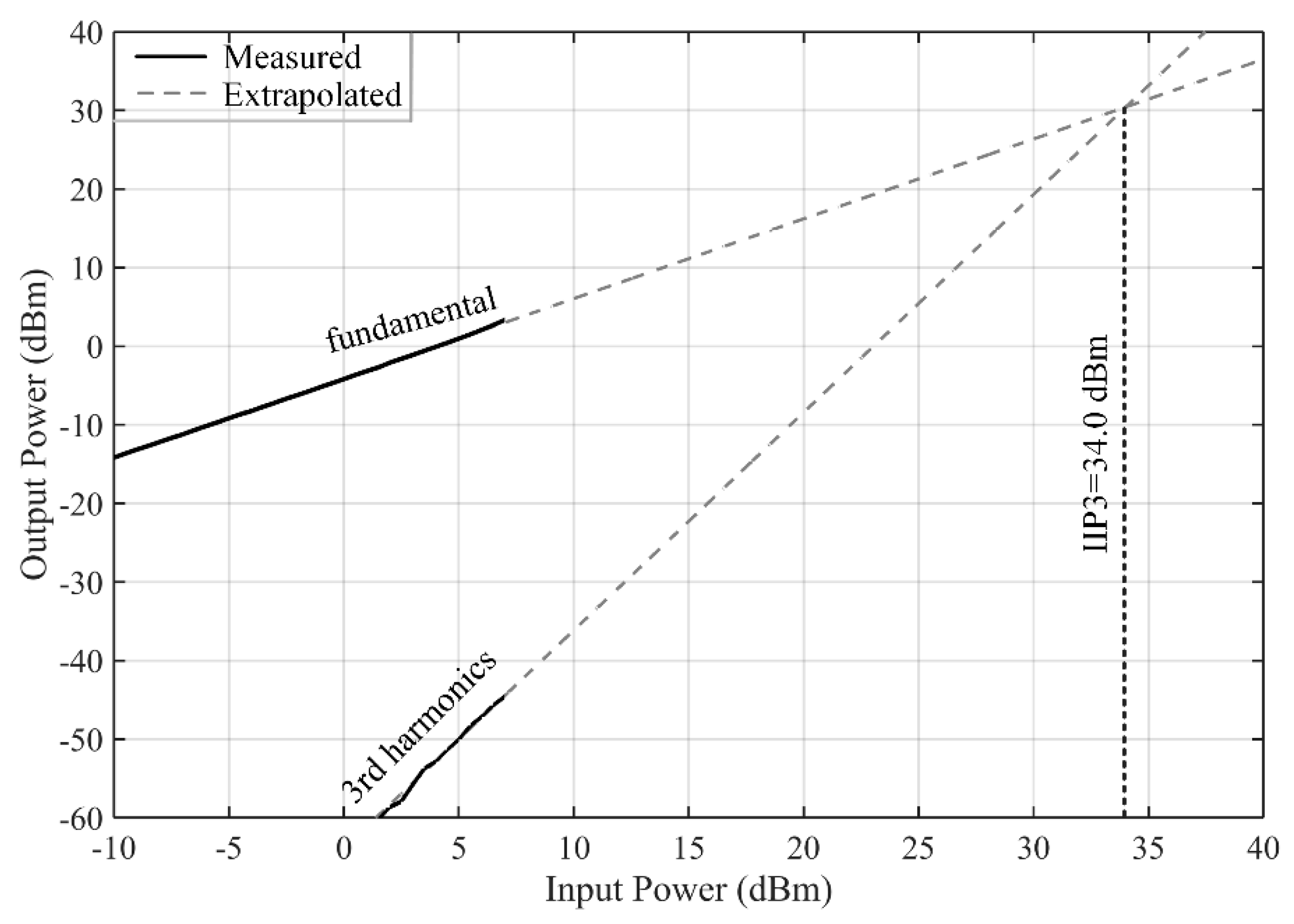
Furthermore, the non-linear characteristics of the system were measured and shown. A third-order intercept point (IIP3) was measured. It is worth mentioning that a varactor is a non-linear device and has a non-linear behavior [25,26]. Two-tone measurements were carried out using 2.4 and 2.41 GHz at the nominal varactor voltage setting. The third harmonics at 2.42 GHz were measured. The calculated IIP3 is shown in Figure 6 and is 34 dBm. The device was tested up to 7 dBm, and in this setting, the insertion losses were measured as −4.1 dB at 2.4 GHz. These insertion losses may vary as the impedance tuner parameters change. This AIMS has shown a high non-linearity parameter, and it is suitable for use in a wide range of medium-/high-power applications.
Lastly, in order to provide a comprehensive perspective, a comparison for the selected relevant publications is shown in Table 2. The tuner performance in this work is not described by a fixed parameter, as it can be switched to a different DUT. This table includes frequency, return loss decision level, and non-linearity test information. In addition, it includes information about the automatic/real-time correction measurements and the antenna impedance adaptation/variation test for the environment changes.
4. Concluding Remarks
An implementation of the AIMS was presented, and testing, validation, and numerical evaluation of the AIMS were shown and discussed. This AIMS can be used for research and development tasks, and it can be applied to medium-/high-power wireless and microwave applications where it needs frequent automatic tuning functions due to the antenna matching variations affected by antenna setting changes. The search approach and numerical evaluations presented in this paper are practical and applicable to a real-time automated matching system. This is an automatic matching system developed for testing and validation. The automatic antenna matching tuning functionality can increase the complexity of the overall system; however, it can provide an adaptable system that provides optimal or best-effort antenna matching conditions. The authors are pursuing further integration of the automatic matching system on a chip. Moreover, authors are investigating the introduction of Python-based instrumentation control applications for the field of testing and validation, and plan to publish more of this broadband matching-related work in near future.
Author Contributions
Conceptualization, B.H., W.R.E, K.L.M.; methodology, B.H., W.R.E, K.L.M.; software, B.H.; validation, B.H.; formal analysis, B.H.; investigation, B.H., W.R.E, K.L.M.; resources, B.H., W.R.E., K.L.M.; data curation, B.H.; writing—original draft preparation, B.H.; writing—review and editing, B.H., W.R.E., K.L.M.; visualization, B.H.; supervision, B.H. and W.R.E.; project administration, B..H, W.R.E., K.L.M.; funding acquisition, B.H., W.R.E., K.L.M.
Funding
This initial research in part was funded by the SRC Global Research Collaboration (GRC) program and Freescale Semiconductor (Theme: 1663.001 and 1836.026, January 2009 ~ Jun 2010). The rest of the research was funded by Hur’s Texas A&M start-up research fund.
Acknowledgments
The authors would like to thank Jaeseok Kim and Hyunjin Park for their prior work and research, and thank Zhen Zhou for her prior work of non-linear property measurements.
Conflicts of Interest
The authors declare no conflict of interest.
References
- Zhang, Y.-M.; Zhang, S.; Li, J.-L.; Pedersen, G.F.; Pedersen, F. A Transmission-Line-Based Decoupling Method for MIMO Antenna Arrays. IEEE Trans. Antennas Propag. 2019, 67, 3117–3131. [Google Scholar] [CrossRef] [Green Version]
- Jha, K.R.; Bukhari, B.; Singh, C.; Mishra, G.; Sharma, S.K. Compact Planar Multistandard MIMO Antenna for IoT Applications. IEEE Trans. Antennas Propag. 2018, 66, 3327–3336. [Google Scholar] [CrossRef]
- Dong, J.; Zhuang, X.; Hu, G. Planar UWB Monopole Antenna with Tri-Band Rejection Characteristics at 3.5/5.5/8 GHz. Information 2019, 10, 10. [Google Scholar] [CrossRef]
- Iqbal, A.; Smida, A.; Mallat, N.K.; Ghayoula, R.; Elfergani, I.; Rodriguez, J.; Kim, S. Frequency and Pattern Reconfigurable Antenna for Emerging Wireless Communication Systems. Electronics 2019, 8, 407. [Google Scholar] [CrossRef]
- Li, R.; Li, B.; Du, G.; Sun, X.; Sun, H. A Compact Broadband Antenna with Dual-Resonance for Implantable Devices. Micromachines 2019, 10, 59. [Google Scholar] [CrossRef] [PubMed]
- Feng, B.; Chung, K.L.; Lai, J.; Zeng, Q. A Conformal Magneto-Electric Dipole Antenna with Wide H-Plane and Band-Notch Radiation Characteristics for Sub-6-GHz 5G Base-Station. IEEE Access 2019, 7, 17469–17479. [Google Scholar] [CrossRef]
- Fano, R. Theoretical limitations on the broadband matching of arbitrary impedances. J. Frankl. Inst. 1950, 249, 139–154. [Google Scholar] [CrossRef]
- Boyle, K.R.; Yuan, Y.; Ligthart, L.P. Analysis of Mobile Phone Antenna Impedance Variations with User Proximity. IEEE Trans. Antennas Propag. 2007, 55, 364–372. [Google Scholar] [CrossRef]
- Kong, F.; Ghovanloo, M.; Durgin, G.D. An Adaptive Impedance Matching Transmitter for a Wireless Intraoral Tongue-Controlled Assistive Technology. IEEE Trans. Circuits Syst. II Express Briefs 2019, 1. [Google Scholar] [CrossRef]
- De Foucauld, E.; Severino, R.; Nicolas, D.; Giry, A.; Delaveaud, C. A 433-MHz SOI CMOS Automatic Impedance Matching Circuit. IEEE Trans. Circuits Syst. II Express Briefs 2018, 66, 958–962. [Google Scholar] [CrossRef]
- Ko, C.-H.; Rebeiz, G.M. A 1.4–2.3-GHz Tunable Diplexer Based on Reconfigurable Matching Networks. IEEE Trans. Microw. Theory Tech. 2015, 63, 1595–1602. [Google Scholar] [CrossRef]
- Lu, P.; Yang, X.-S.; Li, J.-L.; Wang, B.-Z. Polarization Reconfigurable Broadband Rectenna with Tunable Matching Network for Microwave Power Transmission. IEEE Trans. Antennas Propag. 2016, 64, 1. [Google Scholar] [CrossRef]
- Whatley, R.; Zhou, Z.; Melde, K. Reconfigurable RF Impedance Tuner for Match Control in Broadband Wireless Devices. IEEE Trans. Antennas Propag. 2006, 54, 470–478. [Google Scholar] [CrossRef]
- Melde, K.L.; Park, H.-J.; Yeh, H.-H.; Fankem, B.; Zhou, Z.; Eisenstadt, W.R. Software Defined Match Control Circuit Integrated with a Planar Inverted F Antenna. IEEE Trans. Antennas Propag. 2010, 58, 3884–3890. [Google Scholar] [CrossRef]
- Valdovinos, A.; Crespo, A.; Navarro, D.; Garcia, P.; Demingo, J.; De Mingo, J. An RF Electronically Controlled Impedance Tuning Network Design and Its Application to an Antenna Input Impedance Automatic Matching System. IEEE Trans. Microw. Theory Tech. 2004, 52, 489–497. [Google Scholar]
- Kim, J. Automated Matching Control System Using Load Estimation and Microwave Characterization. Ph.D. Dissertation, University of Florida, Gainesville, FL, USA, 2010. [Google Scholar]
- Van Bezooijen, A.; De Jongh, M.; Van Straten, F.; Van Roermund, A.; Mahmoudi, R. Adaptive Impedance-Matching Techniques for Controlling L Networks. IEEE Trans. Circuits Syst. I Regul. Pap. 2009, 57, 495–505. [Google Scholar] [CrossRef]
- Nehring, J.; Schutz, M.; Dietz, M.; Nasr, I.; Aufinger, K.; Weigel, R.; Kissinger, D. Highly Integrated 4–32-GHz Two-Port Vector Network Analyzers for Instrumentation and Biomedical Applications. IEEE Trans. Microw. Theory Tech. 2016, 65, 229–244. [Google Scholar] [CrossRef]
- Nosrati, M.; Daneshmand, M. Gap-Coupled Excitation for Evanescent-Mode Substrate Integrated Waveguide Filters. IEEE Trans. Microw. Theory Tech. 2018, 66, 3028–3035. [Google Scholar] [CrossRef]
- Pal, B.; Mandal, M.K.; Dwari, S. Varactor Tuned Dual-Band Bandpass Filter With Independently Tunable Band Positions. IEEE Microw. Wirel. Components Lett. 2019, 29, 255–257. [Google Scholar] [CrossRef]
- Gilasgar, M.; Barlabe, A.; Pradell, L. A 2.4 GHz CMOS Class-F Power Amplifier with Reconfigurable Load-Impedance Matching. IEEE Trans. Circuits Syst. I Regul. Pap. 2018, 66, 31–42. [Google Scholar] [CrossRef]
- Hur, B.; Eisenstadt, W.R. Tunable Broadband MMIC Active Directional Coupler. IEEE Trans. Microw. Theory Tech. 2012, 61, 168–176. [Google Scholar] [CrossRef]
- Zagorodny, A.S.; Drozdov, A.V.; Voronin, N.N.; Yunusov, I.V. Modeling and application of microwave detector diodes. In Proceedings of the 2013 14th International Conference of Young Specialists on Micro/Nanotechnologies and Electron Devices, Novosibirsk, Russia, 1–5 July 2013; pp. 96–99. [Google Scholar]
- Eisenstadt, W.R.; Hur, B. Embedded RF Test Circuits: RF Power Detectors, RF Power Control Circuits, Directional Couplers, and 77-GHz Six-Port Reflectometer. J. Inf. Commun. Converg. Eng. 2013, 11, 56–61. [Google Scholar] [CrossRef]
- Rogers, J.; Macedo, J.; Plett, C. The effect of varactor nonlinearity on the phase noise of completely integrated VCOs. IEEE J. Solid State Circuits 2000, 35, 1360–1367. [Google Scholar] [CrossRef]
- Scheele, P.; Goelden, F.; Giere, A.; Mueller, S.; Jakoby, R. Continuously tunable impedance matching network using ferroelectric varactors. In Proceedings of the IEEE MTT-S International Microwave Symposium Digest, Long Beach, CA, USA, 17 June 2005. [Google Scholar]
- Sinha, S.; Kumar, A.; Aniruddhan, S. A passive RF impedance tuner for 2.4 GHz ISM band applications. In Proceedings of the 2018 IEEE 19th Wireless and Microwave Technology Conference (WAMICON), Sand Key, FL, USA, 9–10 April 2018. [Google Scholar]
- Baroni, A.; Rogier, H.; Nepa, P. Wearable self-tuning antenna for emergency rescue operations. IET Microw. Antennas Propag. 2016, 10, 173–183. [Google Scholar] [CrossRef]
- Yoon, Y.; Kim, H.; Kim, H.; Lee, K.-S.; Lee, C.-H.; Kenney, J.S. A 2.4-GHz CMOS Power Amplifier with an Integrated Antenna Impedance Mismatch Correction System. IEEE J. Solid State Circuits 2014, 49, 608–621. [Google Scholar] [CrossRef]
- Abdelhalem, S.H.; Gudem, P.S.; Larson, L.E. Tunable CMOS Integrated Duplexer with Antenna Impedance Tracking and High Isolation in the Transmit and Receive Bands. IEEE Trans. Microw. Theory Tech. 2014, 62, 2092–2104. [Google Scholar] [CrossRef]
- Quijano, J.L.A.; Vecchi, G. Optimization of a Compact Frequency- and Environment-Reconfigurable Antenna. IEEE Trans. Antennas Propag. 2012, 60, 2682–2689. [Google Scholar] [CrossRef]
- Song, H.; Bakkaloglu, B.; Aberle, J.T. A CMOS adaptive antenna-impedance-tuning IC operating in the 850MHz-to-2GHz band. In Proceedings of the 2009 IEEE International Solid-State Circuits Conference-Digest of Technical Papers, San Francisco, CA, USA, 8–12 February 2009. [Google Scholar]
- Hoarau, C.; Corrao, N.; Arnould, J.-D.; Ferrari, P.; Xavier, P. Complete Design and Measurement Methodology for a Tunable RF Impedance-Matching Network. IEEE Trans. Microw. Theory Tech. 2008, 56, 2620–2627. [Google Scholar] [CrossRef]
Figure 1.
A generalized conceptual block diagram of the adaptive impedance matching system.

Figure 2.
A functional block diagram of the adaptive broadband impedance matching system (AIMS) implementation in this paper.
Figure 2.
A functional block diagram of the adaptive broadband impedance matching system (AIMS) implementation in this paper.

Figure 3.
A testing and validation system configuration of the AIMS.

Figure 4.
A photograph of the testing and validation system of the AIMS.

Figure 5.
The blue and brown lines show return losses with gaps of (a) 60, (c) 40, and (d) 20 mm. Dark solid lines show automatically tuned return losses, and dashed lines show return loss results before tuning. Dotted lines show the −10 and −12 dB condition. The Smith chart for the non-uniform tuned results with a gap of 60 mm is shown in (b).

Figure 6.
Third-order intercept point (IIP3) measurement at 2.4 GHz.


Table 1.
Numerical evaluations of broadband antenna impedances from 2 to 2.6 GHz.
| Untuned | Tuned | d Δ | |||
|---|---|---|---|---|---|
| 60-nm case (1st attempt) Figure 5a | a Uniform −10 dB | c BW (GHz) | 0.35 | 0.33 | −0.02 |
| AMD (dB) | 1.75 | 2.14 | 0.39 | ||
| SMD (dB) | −4.83 | −3.70 | 1.13 | ||
| b −12 dB & −10 dB | c BW (GHz) | 0.31 | 0.27 | −0.04 | |
| AMD (dB) | 2.01 | 0.61 | −1.40 | ||
| SMD (dB) | −5.12 | −7.31 | −2.19 | ||
| 40-nm case (2nd attempt) Figure 5c | a Uniform −10 dB | c BW (GHz) | 0.26 | 0.33 | 0.07 |
| AMD (dB) | 2.21 | 0.15 | −2.06 | ||
| SMD (dB) | −4.07 | −6.77 | −2.70 | ||
| b−12 dB & −10 dB | c BW (GHz) | 0.31 | 0.34 | 0.03 | |
| AMD (dB) | 0.14 | 0.84 | 0.7 | ||
| SMD (dB) | −7.62 | −6.39 | 1.23 | ||
| 20-nm case (3rd attempt) Figure 5d | a Uniform −10 dB | c BW (GHz) | 0.28 | 0.33 | 0.05 |
| AMD (dB) | 0.27 | −0.30 | −0.57 | ||
| SMD (dB) | −6.65 | −7.37 | −0.72 | ||
| b −12 dB & −10 dB | c BW (GHz) | 0.3 | 0.29 | −0.01 | |
| AMD (dB) | 0.93 | 0.19 | −0.74 | ||
| SMD (dB) | −6.24 | −7.04 | −0.80 |
a decision condition: −10 dB for all the range of frequencies; b decision condition: −12 dB from 2.25 to 2.35 GHz and −10 dB for all the other frequencies; c Effective bandwidth that meets the decision condition; d Subtracted tuned results from untuned results in dB.
Table 2.
Comparison for the selected relevant publications.
| This Work | [27] 2018 | [28] 2016 | [29] 2014 | [30] 2014 | [31] 2012 | [32] 2009 | [33] 2008 | [15] 2004 | ||
|---|---|---|---|---|---|---|---|---|---|---|
| Frequency (GHz) | Band | 2.1 −2.5 | 2.4 −2.5 | 0.406 | 2.4 | 1.7 −2.2 | 1.7 −2.7 | 0.85 −0.2 | 1 | 0.38 −0.43 |
| Multiple band | √ | √ | - | - | √ | √ | √ | - | √ | |
| Return loss (dB) | Uniform decision | <−10 | a- | <−10 | a- | a- | <−10 | a- | <−20 | <−15 |
| Multiple band decision conditions | √ | - | - | - | - | - | - | - | - | |
| Automatic or Real-time correction matching system | √ | - | √ | √ | √ | - | √ | √ | √ | |
| Nonlinearity test such as IIP3 or P1 dB | √ | - | - | √ | √ | - | √ | √ | √ | |
| Antenna Environment Variation/Adaption Test | √ | - | √ | - | - | √ | - | - | √ | |
a-: Not clear to obtain or extract the simple numeric return loss decision value from the publication.
© 2019 by the authors. Licensee MDPI, Basel, Switzerland. This article is an open access article distributed under the terms and conditions of the Creative Commons Attribution (CC BY) license (http://creativecommons.org/licenses/by/4.0/).
Share and Cite
MDPI and ACS Style
Hur, B.; Eisenstadt, W.R.; Melde, K.L. Testing and Validation of Adaptive Impedance Matching System for Broadband Antenna. Electronics 2019, 8, 1055. https://doi.org/10.3390/electronics8091055
AMA Style
Hur B, Eisenstadt WR, Melde KL. Testing and Validation of Adaptive Impedance Matching System for Broadband Antenna. Electronics. 2019; 8(9):1055. https://doi.org/10.3390/electronics8091055
Chicago/Turabian StyleHur, Byul, William R. Eisenstadt, and Kathleen L. Melde. 2019. "Testing and Validation of Adaptive Impedance Matching System for Broadband Antenna" Electronics 8, no. 9: 1055. https://doi.org/10.3390/electronics8091055
Note that from the first issue of 2016, this journal uses article numbers instead of page numbers. See further details here.