Article

Influence of Cold Fronts on Variability of Daily Surface O3 over the Houston-Galveston-Brazoria Area in Texas USA during 2003–2016

1
Department of Earth and Atmospheric Sciences, University of Houston, Houston, TX 77204, USA
2
Institute for Climate and Atmospheric Science, University of Houston, Houston, TX 77204, USA
3
Department of Earth System Science, Tsinghua University, Beijing 100084, China
4
Texas Commission on Environmental Quality, 12100 Park 35 Circle, Austin, TX 78753, USA
*
Author to whom correspondence should be addressed.
Atmosphere 2018, 9(5), 159; https://doi.org/10.3390/atmos9050159
Submission received: 25 March 2018 / Revised: 23 April 2018 / Accepted: 23 April 2018 / Published: 24 April 2018
(This article belongs to the Special Issue Megacities: Air Quality Impacts from Local to Global Scales)

Abstract

:
We investigated the impacts of cold fronts on area-wide peak O 3 and regional background O 3 mixing ratios on a daily scale over the Houston-Galveston-Brazoria (HGB) area of southeastern Texas during the O 3 seasons (April–October) of 2003–2016. Back trajectories showed that an 18h time lag existed between arrival of cold fronts in the HGB area and onset of a predominately northerly flow. Cold fronts showed increasing effects on both peak and background O 3 over the HGB area. Compared to no front days, average peak O 3 mixing ratios during the cold front 1st days, cold front 2+ days, and post frontal days increased 0.7, 5.9, and 9.0 ppbv, respectively while average background O 3 increased 2.9, 6.8, and 8.6 ppbv, respectively. The change in wind direction from southerly to northerly was the most important factor causing increasing O 3 levels. Wind direction shifts caused variation of other meteorological factors (i.e., wind speed, precipitation, temperature, cloud cover, and relative humidity) and tended to overshadow their effects on O 3 over the HGB area. On a long-term and large-scale view, cold fronts over the HGB area could be regarded as interruptions in the cleansing effects of predominantly marine southerly flow from the Gulf of Mexico.

1. Introduction

The influence of cold fronts on surface ozone (O 3 ) is complicated since it can be positive or negative depending on multiple factors such as cold front structure, stage, season, and location. Kunz and Speth [1] discussed three cold front vertical structures and their developments of near-ground O 3 mixing ratios depending upon initial conditions: (1) In winter, O 3 mixing ratios usually increased after a cold front passage because of downward mixing of O 3 -enriched air from the stratosphere into the troposphere by tropopause folding; (2) When folding was less common in summer, O 3 might decrease due to advection of clean air masses or to enhanced cloudiness preventing photochemical production of O 3 , chemical destruction by nitrogen oxides, and heterogeneous chemistry in clouds; (3) O 3 concentrations could remain nearly constant or have a temporary decrease followed by a similar increase when folding was missing.
The influence of cold fronts on surface O 3 exhibits various results in different areas. Chu et al. [2] reported that cold fronts of synoptic weather systems washed out soluble species and advected pollutants out over the Atlantic Ocean. Ott et al. [3] reported a strong inversion over Maryland capping the summer planetary boundary layer (PBL) and limiting downward mixing of stratospheric air helping to preserve low surface O 3 associated with passages of cold fronts that preceded stratospheric intrusions. Yegorova et al. [4] used the Weather Research and Forecasting model with Chemistry (WRF/Chem) to simulate a severe heat wave and smog event on 8–11 July 2007 that were terminated by a cold front. WRF/Chem under-predicted O 3 maxima by 5–8 ppbv where air quality was poor, usually in the northeast, but over-predicted maxima by up to 16 ppbv where O 3 amounts were low, usually in the southeast. Hu et al. [5] simulated a cold front passage in Oklahoma on 3 April 2006 with WRF/Chem. O 3 was at first removed efficiently by chemical reactions then increased rapidly when warmer and O 3 -richer air from aloft was mixed downward to the surface. Leibensperger et al. [6] reported that the frequency of summertime mid-latitude cyclones (and their associated cold fronts) tracking across eastern North America at 40–50 ° N is a strong predictor of stagnation and O 3 pollution days in the eastern US.
As the fourth-largest metropolitan area and one of the most rapidly expanding regions with over 2.3 million inhabitants in the U.S. [7], the Houston area frequently exceeds the National Ambient Air Quality Standards (NAAQS) [8,9,10]. Since 1999, Houston–The Woodlands–Sugar Land metropolitan areas has exchanged titles with Los Angeles as having the most polluted air in the United States defined by the number of days each city violates federal smog standards [11]. Approximately 400 refineries and a multitude of other industrial facilities surround Galveston Bay in the Houston area and contribute to complex and unique emission features [12]. Influence of cold fronts over the Houston-Galveston-Brazoria (HGB) area was a concern in recent years. Lefer et al. [13] reported that several high-O 3 episodes encountered at Moody Tower during the TRAMP campaign (13 August–2 October 2006) were preceded one to two days earlier by a cold front passage, creating a situation where polluted air is transported from the North and interacts with local Houston emissions under light local winds. McMillan et al. [14] and Schade et al. [15] showed from 23 to 30 August 2006, the transport of CO from fires in the United States Pacific Northwest to Houston occurred behind a cold front and contributed to the worst O 3 exceedance period of the summer in the Houston area. Li et al. [16] used surface and aircraft data to validate that observational nudging helped the model yield improved O 3 predictions during a post frontal high O 3 event on 25 September in Houston by reproducing the wind shifts which missed by base case. Pan et al. [17] hypothesized that episodic flare emissions, under dry sunny post frontal stagnated conditions, and land-bay/sea breeze transitions could be a potential cause of high O 3 .
To date, most of the researches on the influence of cold fronts on surface O 3 over the HGB have focused on a single or several cold front events [13,14,15,16,17,18,19,20]. The long-term effect and its mechanism remain unknown. A comprehensive long-term feature of surface O 3 affected by cold fronts over the HGB areas is presented here. In this study, we investigated the impacts of cold fronts on surface peak and background O 3 calculated by the Texas Commission on Environmental Quality (TCEQ) on a daily scale over the HGB area using North American Regional Reanalysis (NARR) meteorology reanalysis data, Weather Prediction Center (WPC) cold front archive, and Hybrid Single Particle Lagrangian Integrated Trajectory (HYSPLIT) model during the O 3 seasons (April–October) of 2003–2016.

2. Data and Methodology
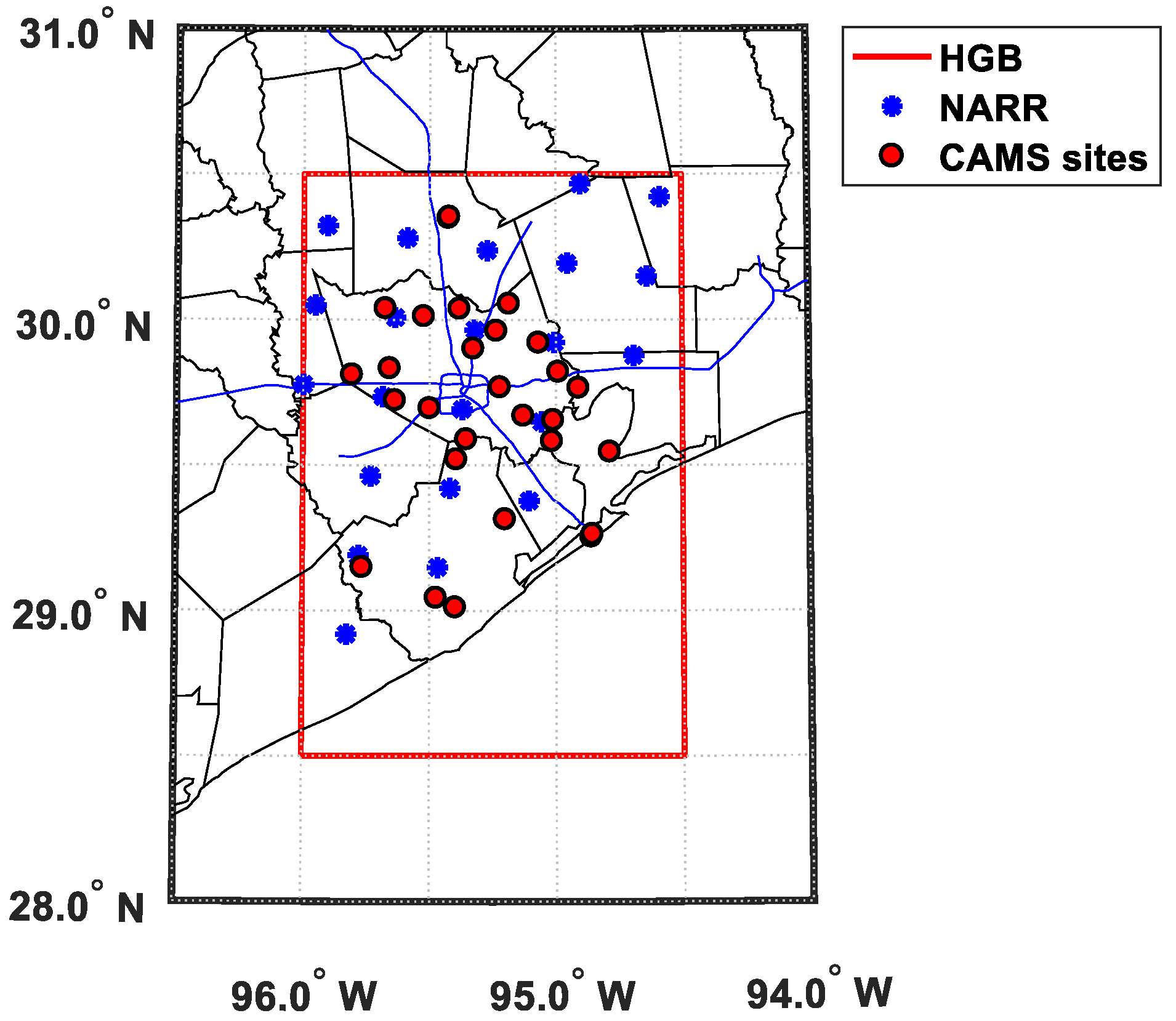
2.1. Study Area

The red box in Figure 1 shows the study area including the region of Houston, Galveston, and Brazoria (HGB), delineated by latitudes of 28.5 ° N to 30.5 ° N, and longitudes of 94.5 ° W to 96.0 ° W.

2.2. O3 and Meteorology

TCEQ calculated daily area-wide peak O 3 and regional background O 3 mixing ratios over the HGB region based on analyses of the daily maximum 8 h average (MDA8) O 3 mixing ratios measured at Continuous Ambient Monitoring Stations (CAMS) (red dots in Figure 1). CAMS sites follow United States Environmental Protection Agency (US EPA) guidelines and some of the sites are registered in EPA network [21]. Regional background O 3 for the HGB area was inferred using the upwind method, as described in detail by Berlin et al. [22]. The O 3 data used here covers the O 3 seasons (April–October) from 2003 to 2016.
The meteorological data (u and v wind components, temperature, precipitation, relative humidity (RH), and cloud cover) over the HGB area were extracted from The National Center for Environmental Prediction (NCEP) and NARR products [23]. The products have a spatial resolution of 32 km × 32 km horizontally with 45 vertical layers, and temporal resolution of every 3 h from 1979 to present, based on observations used in NCEP/NCAR Reanalysis Project. Only grid points (blue “*” in Figure 1) over land in the HGB area were used to calculated daily average meteorological factors.

2.3. Back Trajectory

Back trajectory is the estimation of pollutant transport routine based on wind field. It presents where background O 3 came from in an intuitive way. We used the HYSPLIT model [24] to calculate the back trajectories of air masses at the HGB for April–October from 2003 to 2016. HYSPLIT model is driven by NARR products and calculated every 3 h with 24 h length and the destination height at 100 m above the surface.

2.4. Cold Front Position

Cold front position data was obtained from the WPC Surface Analysis, which is part of the National Weather Service (NWS) Unified Surface Analysis and a collaborative effort with the Ocean Prediction Center (OPC) and the National Hurricane Center (NHC). It is a manual analysis of surface front locations and pressures over North America and adjacent oceans at 3-h intervals and 1 ° × 1 ° spatial resolution from 2003 to present. They utilize a variety of weather data in addition to observations of surface weather conditions, such as upper air observations, global satellite imagery, Doppler radar, and model mass fields to ensure that the product is meteorologically consistent and of the highest quality. Figure S1 shows a sample weather map when a cold front crossed the HGB area.

2.5. Event Days Definitions

A cold front day was defined as the day when a cold front line passed the HGB area in one or more 3-h time frames. Since surface O 3 would be different in independent and continuous cold front days, 1st, 2nd, 3rd … of consecutive days were individually marked as cold front days (i.e., cold front 1st, 2nd, 3rd … days). Some consecutive cold front days that started from a certain cold front day to the end of the cold front episode were merged to be cold front 2+, 3+, … days. Since high O 3 events have been reported after cold front passes [14,15,16,17], post frontal day should be treated as a separate event as well. A post frontal day was defined as the day on which no cold front line passed the HGB area, but the previous day was a cold front day. Cold front days and post frontal days were both defined as cold front related days. A day which had no cold front passage and was not a post frontal day was defined as a no front day.

3. Results

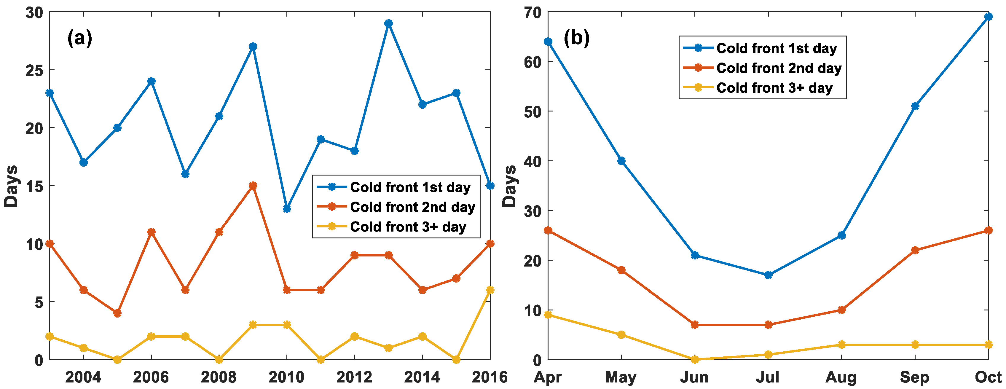
3.1. Cold Front Time Series

Figure 2 shows the time series of cold front days from 2003–2016. There were 427 cold front days during the April–October time frame. Cold front 1st, 2nd and 3+ days totaled 287, 116 and 24 days, respectively. Since only 5.62% of cold front days were cold front 3+ days, we merged cold front 2nd and 3+ day as cold front 2+ days (140 days in total) in the following analysis. The annual time series of cold front counts show no clear trend during the 14-year study period. There were 30.5 cold front days per year during April - October on average. Highest number of cold front days (45 days) happened in 2009 while lowest number of cold front days (22 days) happened in 2010. Monthly time series show that cold front days in summer (JJA) were significantly less than during colder months. In the USA, like most countries located in Northern Hemisphere, northerly wind which brings cold airmass is more frequent during cold months. Cold front is a kind of events featured by northerly wind. It makes sense that cold front in summer is less than cold months.

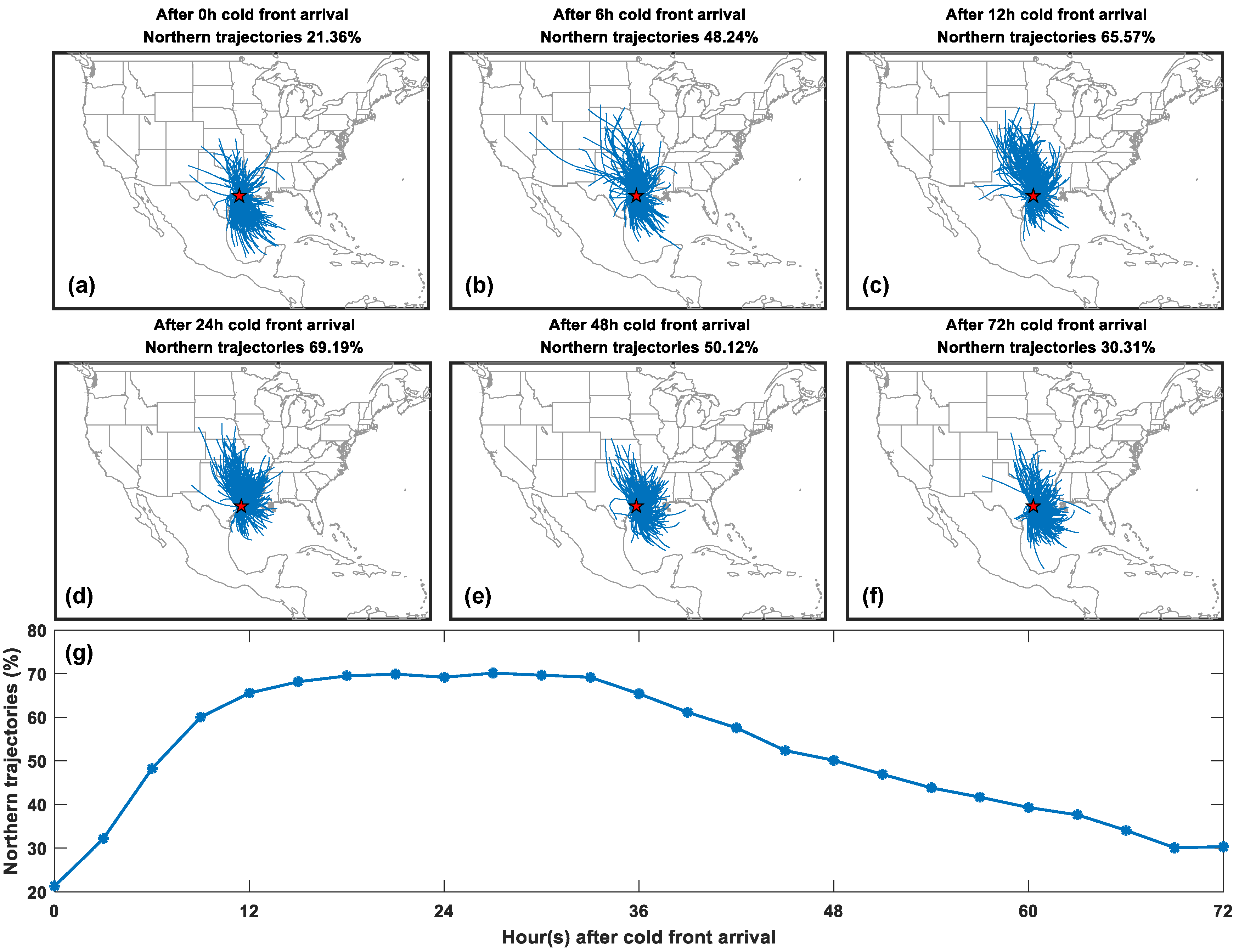
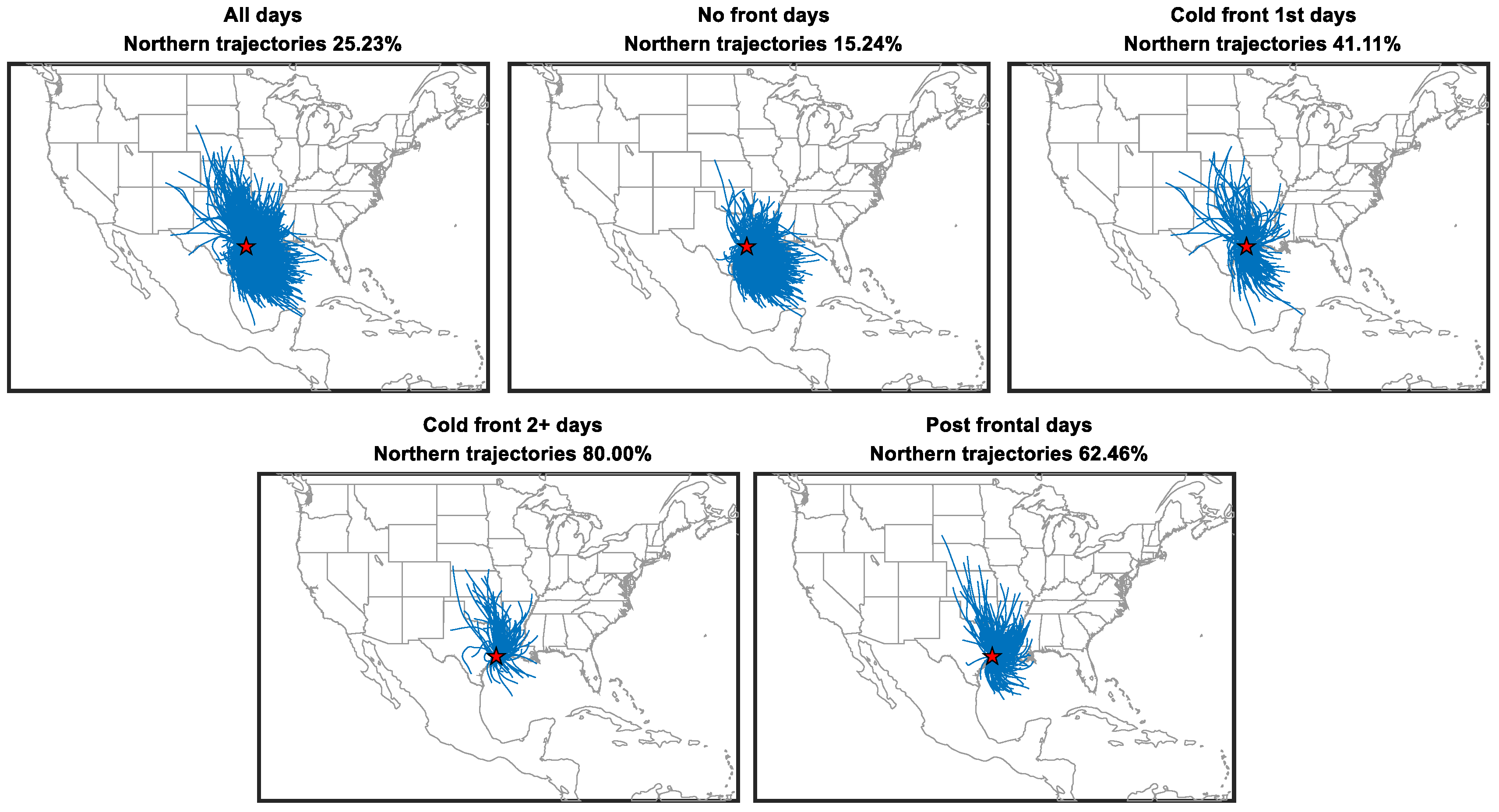
3.2. Back Trajectory
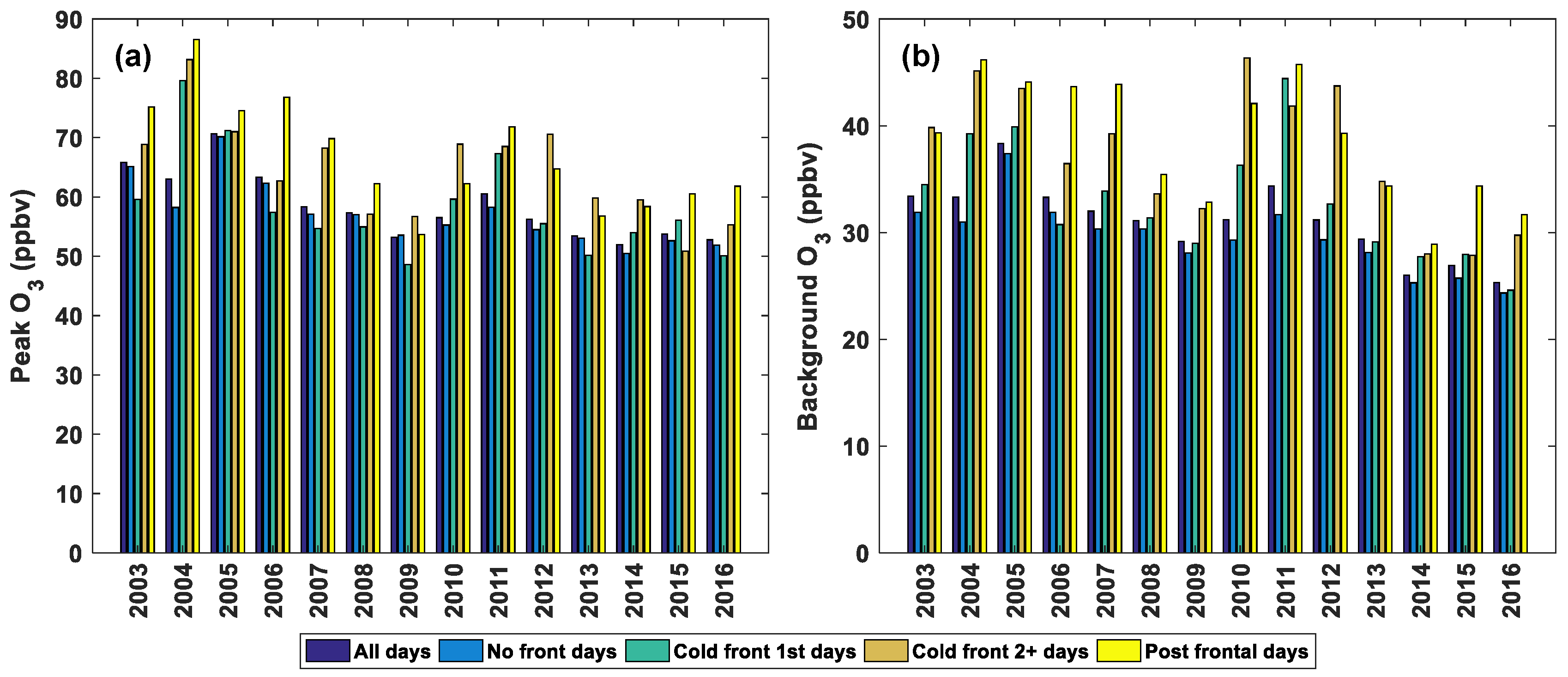
Figure 3a–f shows 24 h back trajectories started at 0, 6, 12, 24, 48, and 72-h after the cold front lines reached the HGB area. For example, a cold front reached the HGB at 15:00 24 April 2004. The back trajectory start hour for this cold front of 0, 6, 12, 24, 48, and 72 h frame are 15:00, 21:00 24 April, 03:00, 15:00 25 April, 15:00 26 April, and 15:00 27 April 2004, respectively. We run every trajectory for 24 h. For example, the trajectory starts at 48 h cover the time 48–72 h after cold front passage and trajectory starts at 72 h cover the time 72–96 h after cold front passage. To study the cold fronts overall behavior, each frame plots all cold fronts in the study period. Since cold fronts would alter wind direction over the HGB from south to north, we can quantify cold front influence by percentage of northern trajectories. We got 8 points other than the start point for each trajectory since 24-h back trajectories run with 3-h resolution. Average latitudes for each trajectory are the mean latitudes of 8 points. A northern trajectory was defined as a trajectory with average latitude greater than its start point (29.72 ° N in this study).
Figure 3g shows the time series of northern trajectories percentage every 3-h. The percentage of northern trajectories rapidly increased from 21.36 to 48.24% in the first 6 h. Then it slowly grew to about 70% about 18 h after the cold front reached the HGB area and kept around 70% until 33 h. In other words, an 18h lag existed between cold front arriving in the HGB area and its influence increasing to the maximum. The maximum influence could continue for about 18h then started to fade. The recovery process after 36 h was much slower than the increasing stage. The northern trajectory percentages were still more than 30% after 72 h the cold front reached the HGB area. It suggests that the influence might be sustained more than 72 h.
Figure 4 shows 24 h back trajectories starting at 15:00 CST during all days, no front days, cold front 1st days, cold front 2+ days, and post frontal days. Both daily regional background O 3 and area-wide peak O 3 , based on MDA8 O 3 , are decided by highest 8 continuous hourly O 3 which usually appears several hours after 12:00 p.m. [16,17,25]. We chose 15:00 CST since the meteorological data is at 3-h interval. Northern trajectories percentages in cold front and post frontal days were much higher than no front days. Notice that northern trajectories percentage in cold front 1st days was about half of cold front 2+ days and 2/3 of post frontal days which suggests the lag between cold front arrival and its influence. The lag might lead to differences in daily O 3 levels among each type of day. To test this hypothesis we examined if O 3 has such a lag as well in the following section.

3.3. O 3 Time Series

Figure 5 shows annual time series of average O 3 mixing ratio. For the whole study period, average peak O 3 during the all days, no front days, cold front 1st days, cold front 2+ days, and post frontal days were 58.4, 57.2, 57.9, 63.0, and 66.2 ppbv, respectively, while average background O 3 mixing ratios were 31.1, 29.7, 32.6, 36.4, and 38.2 ppbv, respectively. Compared to no front days, average peak O 3 mixing ratios during the cold front 1st days, cold front 2+ days, and post frontal days increased 0.7, 5.9, and 9.0 ppbv, respectively while average background O 3 increased 2.9, 6.8, and 8.6 ppbv, respectively. Table S1 shows p values of Two-Sample t-Test of O 3 among each type of event days. p values show that difference of peak O 3 between no front days and cold front 1st days was not significant while it was significant for background O 3 . It suggests that a lag existed between peak and background O 3 increasing. Background O 3 might increase before peak O 3 .
The trends of peak O 3 during all day, no front day, cold front 1st day, cold front 2+ day, and post frontal days were −1.11, −1.06, −1.18, −1.31, and −1.61 ppbv/year, respectively, while the trends of background O 3 were −0.67, −0.64, −0.73, −0.90, and −0.91 ppbv/year, respectively. O 3 during cold front related days deceased faster than on no front days. The changes in regional background O 3 were consistent with trends in northeasterly and southeasterly flow and were −0.50 ± 0.54 and −0.79 ± 0.65 (95% confidence limit) ppbv/yr between 1998 and 2012 [22]. They were also consistent with the summertime downward trend of −0.45 ppbv/year (range of sites: −0.87 to 0.07 ppbv/year) for O 3 in the eastern U.S. between 1990 and 2010 reported by Cooper et al. [26]. They agreed with the estimation of regional background O 3 trend of −0.68 ± 0.27 ppb/year for the period of May–October 1998–2014 reported by Suciu et al. [27] as well.
Figure 6 shows monthly time series of O 3 . Increasing effects of cold front related days on O 3 were more significant during summer than during colder months. O 3 in all days and no front days was usually lower in July due to strong southerly marine inflow caused by the Bermuda High [28]. Low O 3 in July during cold front related days was not clear as no front days since cold front related days are less influenced by southerly flow.

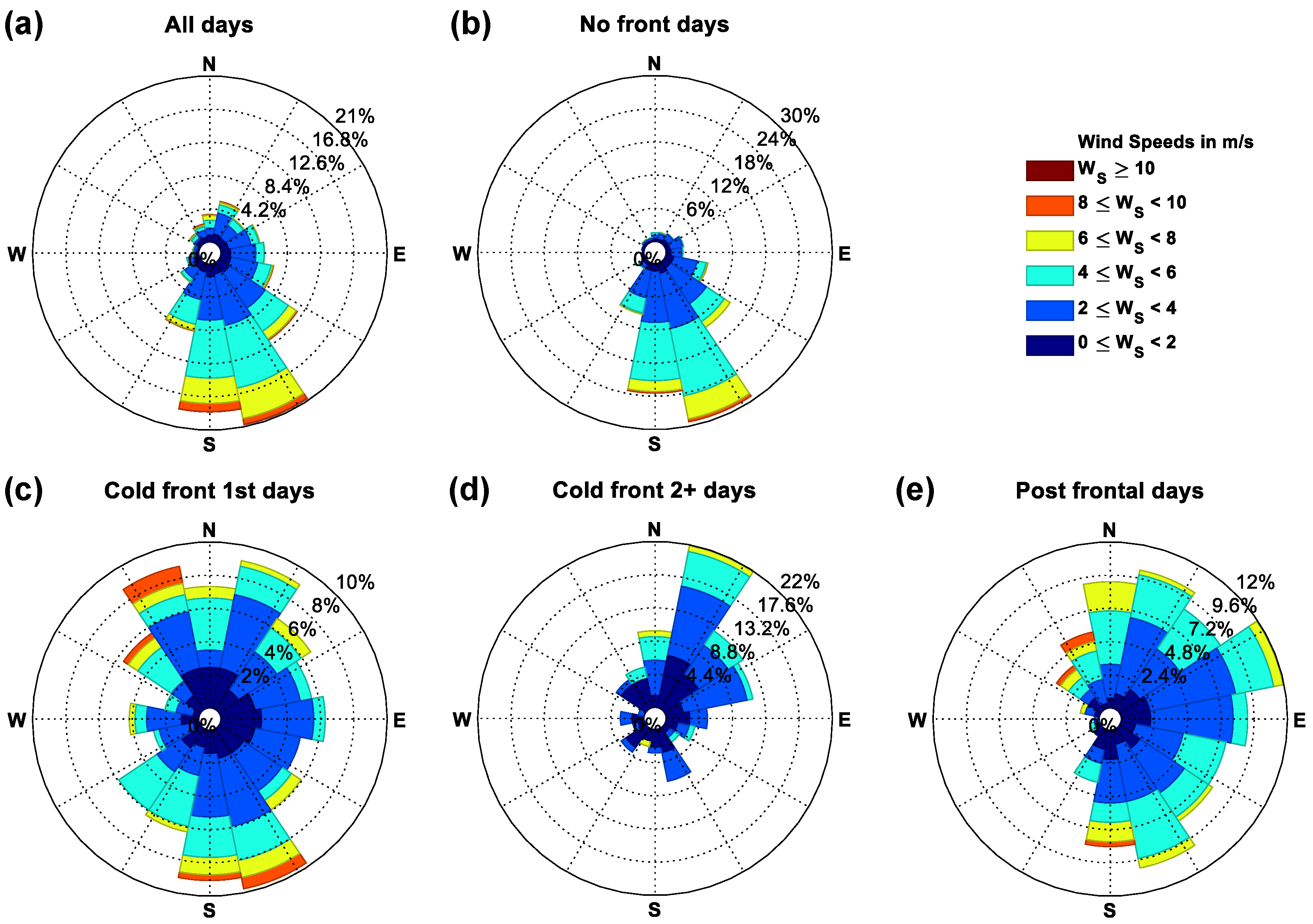
3.4. Meteorology of Cold Front
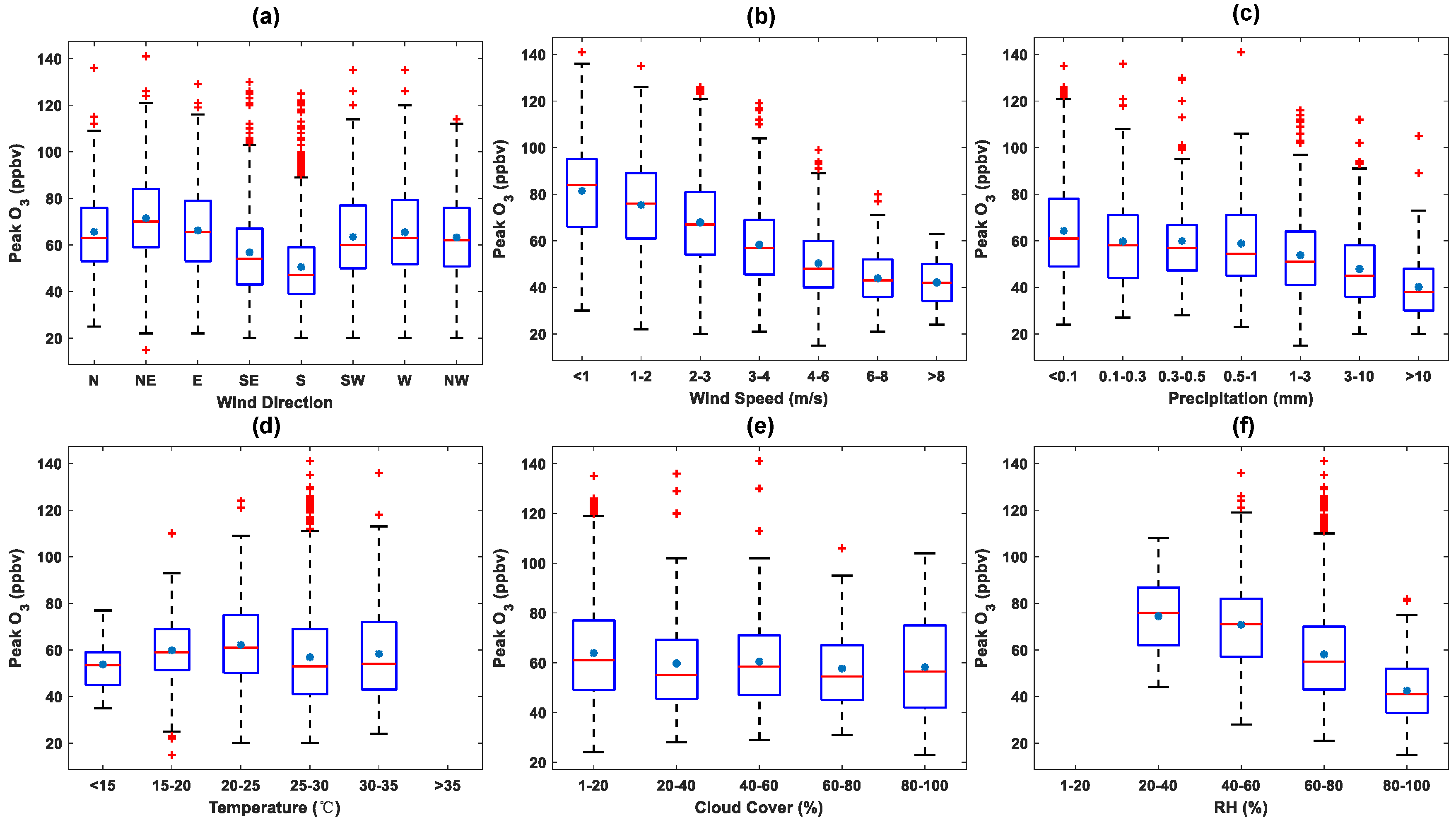
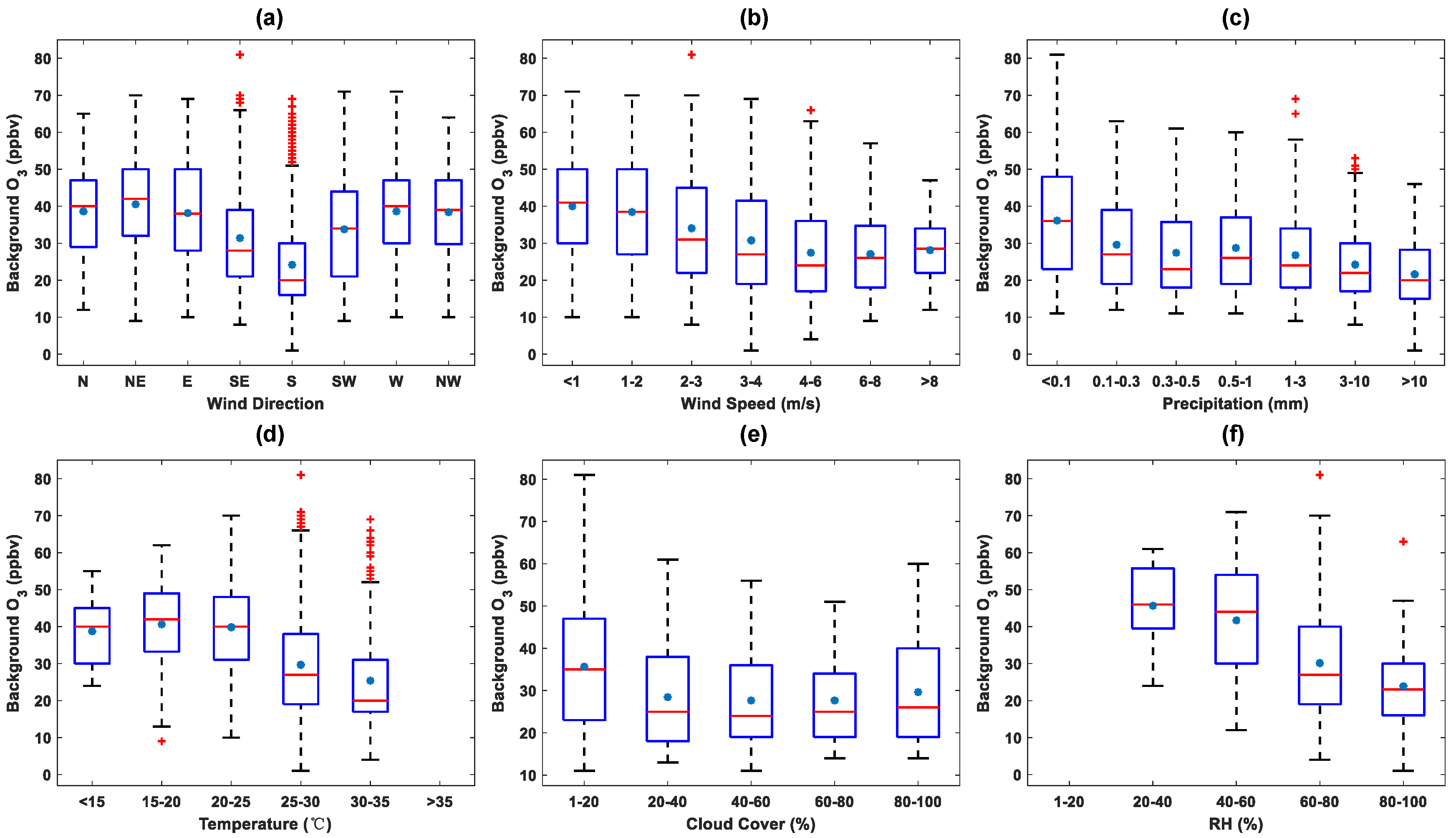
Figure 7 shows the wind rose of daily average wind fields over the HGB area during all days, no front days, cold front 1st days, cold front 2+ days, and post frontal days. We calculated daily average wind u and v components of each NARR grid point, then we calculated daily average wind u and v components of the whole HGB area by averaging wind u and v components of all NARR grid points over the HGB area. Finally, we calculated the daily average wind speed and wind direction based on daily average wind u and v components of the whole HGB area.
In the rose graph of no front days (Figure 7b), general wind directions were from the S (22.2%) and SSE (24.5%). The highest wind speed (10+ m/s) during no front days also occurred in S (0.04%) and SSE (0.09%). Wind speeds were generally between 2–4 m/s (39.8%) and 4–6 m/s (32.3%). During cold front 1st days (Figure 7c) wind from the NNE, N, and NNW increased to 9.1%, 7.3%, and 8.7% respectively. There was no clear major wind direction during cold front 1st days. The highest wind speeds (8–10 m/s) during cold front 1st days occurred in the directions of NNW (1.0%), NW (0.3%), S (0.3%), and SSE (0.7%). Wind speeds were generally between 2-4m/s (41.1%). During cold front 2+ days (Figure 7d), the major wind direction shifted to the NNE (27.1%). The highest wind speeds (8–10 m/s) during cold front 2+ days occurred in the direction of NNE (1.4%) and N (2.1%). During the post frontal days (Figure 7e), winds from the S and SSE (major wind directions during no front days) recovered to 8.4% and 10.2% respectively (about 40% of no front days). It suggests that the influence of cold fronts on wind direction continued during post frontal days. Winds from the east were almost equal to winds from the west during cold front 1st days, while winds from the east side were more than from the west side during post frontal days. These differences suggest the changes between the enhancing and weakening stages of a cold front. The highest wind speed (8–10 m/s) during the post frontal days occurred from the NNW (0.7%), NW (0.4%), and S (0.4%). Wind speeds were generally between 2–4 m/s (43.2%) and 4–6 m/s (30.2%). In summary, there was a lag between cold front arrival and daily average wind fields change. Cold fronts did not completely alter major wind directions on cold front 1st days. Major wind direction shifts from S and SSE to north and NNE on cold front 2+ days. The influence of cold fronts on wind direction continued during post frontal days. Major wind direction during post frontal days might not have recovered by this time to a southerly direction dominant during no front days.
Figure 8 shows box plots of daily average meteorological factors over the HGB area. All box plots in this paper draws points as outliers (red “+” marks) if they are greater than q3 + w × (q3 − q1) or less than q1 − w × (q3 − q1), where w is the maximum whisker length, and q1 and q3 are the 25th and 75th percentiles of the data, respectively. The value for w (Whisker) corresponds to ±2.7 σ (standard deviation) and 99.3% coverage if the data are normally distributed. The plotted whisker extends to the adjacent value, which is the most extreme data value that is not an outlier. Similar to the wind rose analysis, we calculated daily average values (precipitation was daily total in this step) for each NARR grid point, then we calculated daily average values for the whole HGB area by averaging all NARR grid points over the HGB area. Table S2 shows p values of Two-Sample t-Test of meteorology among each type of event days.
For wind speed (Figure 8a), it showed slight variation during front related days. Compared to all no front days, average wind speeds were 0.64, 0.18, and 0.35 m/s lower on cold front 1st days, cold front 2+ days, and post frontal days, respectively. Precipitation (Figure 8b) had an extremely uneven distribution compared to other meteorological factors. For all days in the study period, daily mean precipitation was 2.4 mm and the median was 0.11 mm. Cold front 1st days were significantly higher than other days which suggests that cold fronts passage was a key factor leading to higher precipitation. Average precipitation on cold front 2+ days and post frontal days was 44.2% and 20.2% of cold front 1st days, respectively. For average temperature at 2 m (Figure 8c), it could keep decreasing for several days after arrival of a cold front. Compared to all no front days, average temperature was 1.3, 3.2, and 3.9 ° C lower on cold front 1st days, cold front 2+ days, and post frontal days, respectively. For cloud cover (Figure 8d), it increased on cold front arrival then tended to clear on post frontal days. Compared to no front days, cold front 1st and 2+ days had 7.4% and 5.8% higher cloud cover on average, while post frontal days were 5.0% lower on average. For RH (Figure 8e), its mean value on cold front 1st days was 3.3% and 6.2% higher than on cold front 2+ days and post frontal days, respectively. RH had a clear positive relationship with precipitation but much less range of values.

3.5. O 3 Sensitivity to Meteorology

Unlike other meteorological phenomena, meteorological factors during cold front related days might promote or inhibit O 3 formation if altered individually. For instance, during stagnation days decreasing wind speed and precipitation tend to increase O 3 while during thunderstorm days increasing wind speed and precipitation tend to decrease O 3 . But during cold front related days wind direction shift might bring high background O 3 but decreasing temperature might inhibit O 3 formation. Thus, the final effects of cold front might vary in different areas. To determine which factor was the main cause of increasing O 3 over the HGB area, we tested the sensitivity of O 3 to each meteorological factor (Figure 9 and Figure 10). Unlike modeling studies [29,30], we cannot process sensitivity tests by keeping non-target factors fixed. Thus, the O 3 sensitivity in this study means the O 3 response to a certain meteorological factor under environment conditions in the HGB area.
For wind patterns, peak O 3 was lowest when wind direction (Figure 9a) was the from south (50.6 ppbv) or southeast (56.8 ppbv), which are main wind directions during no front days. It was highest when wind direction was from the northeast (71.5 ppbv), the main wind direction during cold front 2+ days. The impact of wind patterns on surface O 3 in Houston has been reported by [31,32,33,34]. Highest O 3 levels mainly occurred on easterly and northeasterly wind days while increasing southerly flow led to a “cleaner” Houston environment. The wind patterns might be affected by large-scale circulation like the Bermuda High (BH) and Great Plains low level jet (GPLLJ) [28,35], which were both negatively correlated with O 3 over the HGB area. Peak O 3 rose (like wind rose but use O 3 mixing ratio to replace wind speed) in each kind of event days is shown in Figure S2. It shows that in peak O 3 with southernly wind tended to be lower than northerly wind in the same type of event days. Mean peak O 3 decreased from 81.4 ppbv to 43.9 ppbv as the wind speed (Figure 9b) increased from 0 to 8 m/s, but it stopped decreasing when wind speeds were greater than 8 m/s.
Since precipitation (Figure 9c) was extremely unevenly distributed, we grouped precipitation with unequal intervals. Average peak O 3 values decreased from 64.3 ppbv to 40.1 ppbv as precipitation increased from 0 to 10+ mm per day.
Upper limit of peak O 3 increased from 77 to 109 ppbv when temperature (Figure 9d) increased from <15 ° C to 20–25 ° C but stopped increasing when temperatures rose higher. In fact, there was no clear trends in median or mean values of peak O 3 as temperatures rose. Rising temperature might cause O 3 exceedance in extreme events like heatwaves [36,37] but the sensitivity of surface O 3 to large-scale warming was highly variable owing to variation in advection of regional O 3 [38]. Air temperature was most strongly correlated with O 3 north of 38 ° N (>0.7) and weakened south of 36 ° N (<0.5) over the Eastern United States (US) (including the HGB area) for August from 1994 to 2010 [39].
For cloud cover (Figure 9e), the mean of peak O 3 had no clear change when cloud cover increased. The upper limit of peak O 3 was significantly lower when cloud cover was greater than 20% except for some outliers. O 3 photochemistry is photon-limited. Cloud cover affects surface O 3 by blocking sunlight. Cloud cover was reported -1.05 ppbv surface O 3 per 10% change [40].
Average of peak O 3 decreased from 74.4 ppbv to 42.54 ppbv when RH (Figure 9f) increased from 20-40% to 80-100%. It is consistent with the O 3 -RH correlation that transitioning from positive to negative south of 37 ° N [39]. The O 3 /RH regression slopes in Huntsville, AL, during the peak O 3 season (May to September) in 2013 were −1.0, −0.6, −0.5, and −3.6 ppb/% for the surface, PBL, mid-troposphere, and upper troposphere, respectively [41]. O 3 anomalies (deviation from normal value) reached +12 ppb from 30 to 36 ° N in 1999, and 4–7 ppb higher, during the historic 2007 drought in the Southeastern United States (U.S.) [39,42].
Mean background O 3 was lowest when wind direction (Figure 10a) was from the south (24.2 ppbv), while it was highest when wind direction was from the northeast (40.5 ppbv). Background O 3 rose in each kind of event days is shown in Figure S3. Background O 3 rose shows similar results with Peak O 3 rose. Background O 3 from north tended to be higher than from south in the same kind of event days. Mean background O 3 decreased from 40.0 ppbv to 27.5 ppbv as the wind speed (Figure 10b) increased from 0–1 to 4–6 m/s while the upper limit was stable around 70 ppbv when wind speed was <4 m/s. Mean background O 3 stopped increasing when wind speed increased from 4–6 to >8 m/s. The upper limit decreased from 70 ppbv to 47 ppbv when wind speed increased from 3–4 to >8 m/s.
The median value of background O 3 decreased sharply from 36 ppbv to 27 ppbv as precipitation (Figure 10c) increased from 0–0.1 to 0.1–0.3 mm per day then was stable when precipitation increased from 0.1–0.3 to 0.5–1 mm per day. It decreased again when precipitation was greater than 1 mm per day. The upper limit of background O 3 kept decreasing from 81 ppbv to 46 ppbv as precipitation increased from 0–10+ mm per day.
The mean of background O 3 increased sharply from 25.4 ppbv to 39.8 ppbv when temperature (Figure 10d) decreased from 30–35 ° C to 20–25 ° C. This is likely due to cold fronts bringing high background O 3 and low temperatures simultaneously, O 3 had no clear change when temperature decreased further.
The upper limit of background O 3 decreased steadily from 81 ppbv to 51 ppbv when cloud cover (Figure 10e) increased from 0 to 80%. The mean value of background O 3 was lower when cloud cover was >20%, though it had no clear change when cloud cover increased from 20 to 80%. Background O 3 increased when cloud cover increased from 80%-100%. This is likely due to fact that cold fronts caused high background O 3 and cloud cover at the same time. Similar to peak O 3 , average background O 3 decreased from 45.7 ppbv to 23.9 ppbv when RH (Figure 10f) increased from 20–40% to 80–100%.

4. Discussion

To understand how cold fronts affect O 3 over the HGB, we need to combine the meteorology of cold fronts with O 3 sensitivity to meteorology. Considering the extremely uneven distribution of precipitation, we show median not mean difference here. Table 1 shows median difference of meteorology compared to no front days. For wind direction, we calculated median u and v wind components during the same type of days and the median wind directions were derived based on the median u and v wind components. For other meteorological factors, we used median values during different type of days in Figure 8. Table 2 shows O 3 difference caused by meteorology compared to no front days. For wind direction, we calculated the O 3 difference based on the difference of median wind direction during different type of days in Figure 9 and Figure 10. For other meteorological factors, we calculated linear regression slopes of data in Figure 9 and Figure 10. Parameters of linear regression are shown in Table S3. Then we calculated O 3 difference by timing slopes and median difference of meteorology in Table 1. The uncertainties are estimated based on 95% confidence intervals in Table S3 except for wind direction since the ozone difference caused by wind direction cannot be estimated by linear regression. The uncertainties are huge because of the big range of meteorology. Since O 3 response to meteorology is not linear in reality, the results of O 3 difference can be used for qualitative reference only. To get better estimations for such a non-linear problem, research based on atmospheric chemistry transport models (CTMs) needs to be done in the future.
For wind patterns, shifts in wind direction should be the major factor that affects O 3 during cold front related days. In no front days, wind usually came from the south, the direction of the Gulf of Mexico which is less influenced by human activities compared to inland area. Major wind direction shifted from south to north or northeast after cold front passage bringing high background from inland area.
Changes of other meteorological factors during cold front events could be regarded as the consequence of wind direction shift. O 3 differences caused by wind direction were much greater than other factors (Table 2). On a daily average level, a lag existed between cold front arrival and daily average wind direction change (Figure 7). This is the reason why high background O 3 advected by cold fronts raised peak O 3 starting on cold front 1st days while the main wind direction during cold front 1st days was still south or southeast. On the other hand, O 3 decreased rapidly as wind speed increased (Figure 9b and Figure 10b), but the median value of wind speed during cold front days decreased less than 1 m/s (Figure 8a). Thus, wind speed was not a key factor increasing O 3 during cold front related days.
For precipitation, O 3 decreased rapidly as precipitation increased (Figure 9c and Figure 10c). Daily mean precipitation exhibited an extremely uneven distribution (Figure 8b). The number of high precipitation days was much less than low or no precipitation days. This is likely the reason why precipitation showed an overall small effect on O 3 . Precipitation during cold front 1st days was much higher than on other days. This could be the reason why O 3 during cold front 1st days was lower than cold front 2+ days and post front days.
For temperature, usually it shows positive correlation with O 3 [39]. Depressed temperatures decreased the upper limit of peak O 3 but did not reduce the mean and median values of peak O 3 (Figure 9d). On the other hand, depressed temperatures unusually increased the mean and median values of background O 3 (Figure 10d). Note that cold fronts decreased temperature and brought high background O 3 through changes in wind direction at the same time. This implies that temperature effects might be overshadowed by changes in wind direction. It also helps to explain why depressed temperatures showed increasing effects on O 3 levels (Table 2).
For cloud cover, mean values were higher than on other days during cold front days and lower during post frontal days (Figure 8d). Both peak and background O 3 over the HGB area were not sensitive to cloud cover (Figure 9e and Figure 10e). Thus, cloud cover does not appear to be a key factor affecting O 3 during cold front related days.
For RH, both peak and background O 3 values over the HGB area decreased significantly when RH increased from 20% to 100% (Figure 9f and Figure 10f). RH increased a little as precipitation during cold front 1st days then decreased since dry air brought by in-land northerly flow during cold front 2+ days and post frontal days. Overall mean RH always stays at a relatively high level (Figure 8e) since the HGB area is close to the Gulf of Mexico. Variation of mean RH was less than 5% as the cold front passes. Thus, RH influence on O 3 during cold front related days was not as significant as O 3 sensitivity to RH.
In summary, high background O 3 was brought to the HGB area by wind direction shifts to inland advection pathways. This was the key factor increasing peak and background O 3 during cold front related days. Wind direction shifts caused variation of other meteorological factors and overshadowed their effects on O 3 . Independent high O 3 incidents related to cold fronts over the HGB area were studied in previous works [13,14,15,16,17,18,19,20]. The usual explanations for increased O 3 involved air mass stagnation, under cloud free conditions caused by wind direction shifts. On a long-term and large-scale view, cold fronts could be regarded as interruptions of a “normal” circulation system. It enhanced surface O 3 over the HGB area temporarily by interrupting the cleansing effect of southerly marine flow which was the predominant wind direction on cold front related days. This same effect might also affect other metro areas near south coast in subtropics controlled by similar circulation systems [43].

5. Summary and Conclusions

In this study, we investigated the impacts of cold fronts on surface peak and background O 3 calculated by TCEQ method on a daily scale using NARR meteorology reanalysis data, the WPC cold front archive, and HYSPLIT back trajectory model during O 3 seasons (April–October) 2003–2016. Cold front passage is a transient event, but its impacts may continue in the following days. There were 427 cold front days during research period and about 40% of them occurred for 2 or more continuous days. Back trajectory analysis shows an 18h lag exists between cold front arrival in the HGB area and the percentage of northerly trajectories increasing to about 70%. The percentage kept stable for about 18 h then decreased slowly. This time frame could last more than 72h after cold fronts arrival. Northern trajectories percentage during cold front 1st days was significantly less than cold front 2+ days and post frontal days though it was 2.7 times as no front days.
Cold fronts showed increasing effects on both peak and background O 3 over the HGB area. Compared to no front days, average peak O 3 mixing ratios during the cold front 1st days, cold front 2+ days, and post frontal days increased 0.7, 5.9, and 9.0 ppbv, respectively while average background O 3 increased 2.9, 6.8, and 8.6 ppbv, respectively. The annual decreasing trend of O 3 during cold front related days was larger than no front days. Since O 3 during cold front related days is more heavily affected by anthropogenic sources compared to no front days usually with clean southernly flow, it suggests that cutting down anthropogenic emission of O 3 precursors may have played a more important role in reducing the O 3 exceedances than increasing southerly flow [33]. Over the HGB area, average O 3 was lower during southern flow days especially in summer [28]. It might be the reason why cold fronts caused larger background O 3 differences between cold front related days and no front days in summer (JJA) than in cooler months.
Analysis of meteorology and O 3 sensitivity shows that wind direction change was the key factor causing increasing O 3 levels. Cold fronts shifted the main wind direction from the south and southeast to the north and northeast, which consequently brought high background O 3 from inland areas. Wind direction shifts caused the change in air mass and variations of other meteorological factors (wind speed, precipitation, temperature, cloud cover, and RH). The effects of wind direction shifts overshadowed other effects on O 3 over the HGB area.
The impact of cold frontal passage upon O 3 is complex since meteorological factors altered by cold frontal dynamics could inhibit or promote O 3 formation if they happened individually. Thus, the final impact of cold fronts on O 3 could be varied spatially and temporally. On a long-term and large-scale view, cold fronts over the HGB area could be regarded as interruptions of the cleansing effect of predominant marine southerly-flow from the Gulf of Mexico. The HGB area could share the same situation with other metro areas near the Gulf Coast. Comparison among the HGB area and other types of cities remains to be done. High-resolution cold front data is still lacking to study cold frontal passage within the city. Differences among cold front types need further study as well.

Supplementary Materials

The following are available online at https://www.mdpi.com/2073-4433/9/5/159/s1, Figure S1. Sample weather map of the WPC surface analysis valid for 04/04/2014 at 12 UTC, Figure S2: Peak O 3 rose during (a) all days, (b) no front days, (c) cold front 1st days, (d) cold front 2+ days, and (e) post frontal days, Figure S3: Background O 3 rose during (a) all days, (b) no front days, (c) cold front 1st days, (d) cold front 2+ days, and (e) post frontal days, Table S1. P values of Two-Sample t-Test of O 3 among each type of event days, Table S2. P values of Two-Sample t-Test of meteorology among each type of event days, Table S3. Linear regression parameters of O 3 vs. meteorological factors.

Author Contributions

Ruixue Lei (data collection, data analysis, manuscript writing); Robert Talbot (manuscript writing); Yuxuan Wang (data collection, manuscript writing); Sing-Chun Wang (data analysis, manuscript proofing); Mark Estes (data collection, manuscript proofing).

Acknowledgments

This work was funded by a grant from the Texas Air Quality Research Program (AQRP 16-008) at The University of Texas at Austin through the Texas Emission Reduction Program (TERP) and the Texas Commission on Environmental Quality (TCEQ). The findings, opinions and conclusions are the work of the author(s) and do not necessarily represent findings, opinions, or conclusions of the AQRP or the TCEQ. We thank National Oceanic and Atmospheric Administration (NOAA)/National Weather Service (NWS) Weather Prediction Center for providing the cold front data. We also thank the University of Houston Center for Advanced Computing and Data Science for providing computational resources.

Conflicts of Interest

The authors declare no conflict of interest.

References

  1. Kunz, H.; Speth, P. Variability of near-ground ozone concentrations during cold front passages—A possible effect of tropopause folding events. J. Atmos. Chem. 1997, 28, 77–95. [Google Scholar] [CrossRef]
  2. Chu, D.A.; Ferrare, R.; Szykman, J.; Lewis, J.; Scarino, A.; Hains, J.; Burton, S.; Chen, G.; Tsai, T.; Hostetler, C.; et al. Regional characteristics of the relationship between columnar AOD and surface PM2.5: Application of lidar aerosol extinction profiles over Baltimore–Washington Corridor during DISCOVER-AQ. Atmos. Environ. 2015, 101, 338–349. [Google Scholar] [CrossRef]
  3. Ott, L.E.; Duncan, B.N.; Thompson, A.M.; Diskin, G.; Fasnacht, Z.; Langford, A.O.; Lin, M.; Molod, A.M.; Nielsen, J.E.; Pusede, S.E.; et al. Frequency and impact of summertime stratospheric intrusions over Maryland during DISCOVER-AQ (2011): New evidence from NASA’s GEOS-5 simulations. J. Geophys. Res. Atmos. 2016, 121, 3687–3706. [Google Scholar] [CrossRef]
  4. Yegorova, E.; Allen, D.; Loughner, C.; Pickering, K.; Dickerson, R. Characterization of an eastern US severe air pollution episode using WRF/Chem. J. Geophys. Res. Atmos. 2011, 116, D17306. [Google Scholar] [CrossRef]
  5. Hu, X.M.; Klein, P.M.; Xue, M.; Shapiro, A.; Nallapareddy, A. Enhanced vertical mixing associated with a nocturnal cold front passage and its impact on near-surface temperature and ozone concentration. J. Geophys. Res. Atmos. 2013, 118, 2714–2728. [Google Scholar] [CrossRef]
  6. Leibensperger, E.M.; Mickley, L.J.; Jacob, D.J. Sensitivity of US air quality to mid-latitude cyclone frequency and implications of 1980–2006 climate change. Atmos. Chem. Phys. 2008, 8, 7075–7086. [Google Scholar] [CrossRef]
  7. U.S. Census Bureau, P.D. Metropolitan and Micropolitan Statistical Area Population and Estimated Components of Change: April 1, 2010 to July 1, 2016 (CBSA-EST2016-alldata). 2017. Available online: https://www.census.gov/data/tables/2016/demo/popest/total-metro-and-micro-statistical-areas.html (accessed on 1 May 2017).
  8. U.S. EPA. 2008 National Ambient Air Quality Standards (NAAQS) for Ozone. Available online: https://www.epa.gov/ozone-pollution/2008-national-ambient-air-quality-standards-naaqs-ozone (accessed on 1 May 2017).
  9. U.S. EPA. 2015 National Ambient Air Quality Standards (NAAQS) for Ozone. Available online: https://www.epa.gov/ozone-pollution/2015-national-ambient-air-quality-standards-naaqs-ozone#rule-summary (accessed on 1 May 2017).
  10. Cuchiara, G.C.; Li, X.; Carvalho, J.; Rappenglück, B. Intercomparison of planetary boundary layer parameterization and its impacts on surface ozone concentration in the WRF/Chem model for a case study in Houston/Texas. Atmos. Environ. 2014, 96, 175–185. [Google Scholar] [CrossRef]
  11. Wilson, J. Getting the Big Picture on Houston’s Air Pollution. Available online: http://www.nasa.gov/vision/earth/everydaylife/archives/HP_ILP_Feature_03.html (accessed on 1 May 2017).
  12. Levy, M.E.; Zhang, R.; Khalizov, A.F.; Zheng, J.; Collins, D.R.; Glen, C.R.; Wang, Y.; Yu, X.Y.; Luke, W.; Jayne, J.T.; et al. Measurements of submicron aerosols in Houston, Texas during the 2009 SHARP field campaign. J. Geophys. Res. Atmos. 2013, 118, 10518–10534. [Google Scholar] [CrossRef]
  13. Lefer, B.; Rappenglück, B.; Flynn, J.; Haman, C. Photochemical and meteorological relationships during the Texas-II Radical and Aerosol Measurement Project (TRAMP). Atmos. Environ. 2010, 44, 4005–4013. [Google Scholar] [CrossRef]
  14. McMillan, W.; Pierce, R.; Sparling, L.; Osterman, G.; McCann, K.; Fischer, M.; Rappenglueck, B.; Newsom, R.; Turner, D.; Kittaka, C.; et al. An observational and modeling strategy to investigate the impact of remote sources on local air quality: A Houston, Texas, case study from the Second Texas Air Quality Study (TexAQS II). J. Geophys. Res. Atmos. 2010, 115, D01301. [Google Scholar] [CrossRef]
  15. Schade, G.W.; Khan, S.; Park, C.; Boedeker, I. Rural southeast texas air quality measurements during the 2006 texas air quality study. J. Air Waste Manag. Assoc. 2011, 61, 1070–1081. [Google Scholar] [CrossRef] [PubMed]
  16. Li, X.; Choi, Y.; Czader, B.; Roy, A.; Kim, H.; Lefer, B.; Pan, S. The impact of observation nudging on simulated meteorology and ozone concentrations during DISCOVER-AQ 2013 Texas campaign. Atmos. Chem. Phys. 2016, 16, 3127–3144. [Google Scholar] [CrossRef]
  17. Pan, S.; Choi, Y.; Jeon, W.; Roy, A.; Westenbarger, D.A.; Kim, H.C. Impact of high-resolution sea surface temperature, emission spikes and wind on simulated surface ozone in Houston, Texas during a high ozone episode. Atmos. Environ. 2017, 152, 362–376. [Google Scholar] [CrossRef]
  18. Banta, R.; Senff, C.; Nielsen-Gammon, J.; Darby, L.; Ryerson, T.; Alvarez, R.; Sandberg, S.; Williams, E.; Trainer, M. A bad air day in Houston. Bull. Am. Meteorol. Soc. 2005, 86, 657–669. [Google Scholar] [CrossRef]
  19. Haman, C.; Couzo, E.; Flynn, J.; Vizuete, W.; Heffron, B.; Lefer, B. Relationship between boundary layer heights and growth rates with ground-level ozone in Houston, Texas. J. Geophys. Res. Atmos. 2014, 119, 6230–6245. [Google Scholar] [CrossRef]
  20. Langford, A.; Senff, C.; Banta, R.; Hardesty, R.; Alvarez, R.; Sandberg, S.P.; Darby, L.S. Regional and local background ozone in Houston during Texas Air Quality Study 2006. J. Geophys. Res. Atmos. 2009, 114, D00F12. [Google Scholar] [CrossRef]
  21. What Is a CAMS? Available online: https://www.tceq.texas.gov/cgi-bin/compliance/monops/daily_info.pl?cams (accessed on 1 May 2017).
  22. Berlin, S.R.; Langford, A.O.; Estes, M.; Dong, M.; Parrish, D.D. Magnitude, decadal changes, and impact of regional background ozone transported into the Greater Houston, Texas, area. Environ. Sci. Technol. 2013, 47, 13985–13992. [Google Scholar] [CrossRef] [PubMed]
  23. National Centers for Environmental Prediction; National Weather Service; NOAA; U.S. Department of Commerce (2005): NCEP North American Regional Reanalysis (NARR). Research Data Archive at the National Center for Atmospheric Research, Computational and Information Systems Laboratory. Available online: http://rda.ucar.edu/datasets/ds608.0/ (accessed on 1 May 2017).
  24. Stein, A.; Draxler, R.R.; Rolph, G.D.; Stunder, B.J.; Cohen, M.; Ngan, F. NOAA’s HYSPLIT atmospheric transport and dispersion modeling system. Bull. Am. Meteorol. Soc. 2015, 96, 2059–2077. [Google Scholar] [CrossRef]
  25. Baier, B.C.; Brune, W.H.; Lefer, B.L.; Miller, D.O.; Martins, D.K. Direct ozone production rate measurements and their use in assessing ozone source and receptor regions for Houston in 2013. Atmos. Environ. 2015, 114, 83–91. [Google Scholar] [CrossRef]
  26. Cooper, O.R.; Gao, R.S.; Tarasick, D.; Leblanc, T.; Sweeney, C. Long-term ozone trends at rural ozone monitoring sites across the United States, 1990–2010. J. Geophys. Res. Atmos. 2012, 117. [Google Scholar] [CrossRef]
  27. Suciu, L.G.; Griffin, R.J.; Masiello, C.A. Regional background O3 and NOx in the Houston–Galveston– Brazoria (TX) region: A decadal-scale perspective. Atmos. Chem. Phys. 2017, 17, 6565–6581. [Google Scholar] [CrossRef]
  28. Wang, Y.; Jia, B.; Wang, S.C.; Estes, M.; Shen, L.; Xie, Y. Influence of the Bermuda High on interannual variability of summertime ozone in the Houston–Galveston–Brazoria region. Atmos. Chem. Phys. 2016, 16, 15265–15276. [Google Scholar] [CrossRef]
  29. Johnson, M.S.; Kuang, S.; Wang, L.; Newchurch, M.J. Evaluating summer-time ozone enhancement events in the southeast United States. Atmosphere 2016, 7, 108. [Google Scholar] [CrossRef]
  30. Kim, E.; Kim, B.U.; Kim, H.C.; Kim, S. The Variability of Ozone Sensitivity to Anthropogenic Emissions with Biogenic Emissions Modeled by MEGAN and BEIS3. Atmosphere 2017, 8, 187. [Google Scholar] [CrossRef]
  31. Souri, A.H.; Choi, Y.; Li, X.; Kotsakis, A.; Jiang, X. A 15-year climatology of wind pattern impacts on surface ozone in Houston, Texas. Atmos. Res. 2016, 174, 124–134. [Google Scholar] [CrossRef]
  32. Nielsen-Gammon, J.; Tobin, J.; McNeel, A.; Li, G. A Conceptual Model for Eight-Hour Ozone Exceedances in Houston, Texas Part I: Background Ozone Levels in Eastern Texas. Available online: http://oaktrust.library.tamu.edu/handle/1969.1/158250 (accessed on 1 May 2017).
  33. Liu, L.; Talbot, R.; Lan, X. Influence of climate change and meteorological factors on Houston’s air pollution: ozone a case study. Atmosphere 2015, 6, 623–640. [Google Scholar] [CrossRef]
  34. Pakalapati, S.; Beaver, S.; Romagnoli, J.A.; Palazoglu, A. Sequencing diurnal air flow patterns for ozone exposure assessment around Houston, Texas. Atmos. Environ. 2009, 43, 715–723. [Google Scholar] [CrossRef]
  35. Shen, L.; Mickley, L.; Tai, A. Influence of synoptic patterns on surface ozone variability over the eastern United States from 1980 to 2012. Atmos. Chem. Phys. 2015, 15, 10925–10938. [Google Scholar] [CrossRef]
  36. Pu, X.; Wang, T.; Huang, X.; Melas, D.; Zanis, P.; Papanastasiou, D.; Poupkou, A. Enhanced surface ozone during the heat wave of 2013 in Yangtze River Delta region, China. Sci. Total Environ. 2017, 603, 807–816. [Google Scholar] [CrossRef] [PubMed]
  37. Hou, P.; Wu, S. Long-term changes in extreme air pollution meteorology and the implications for air quality. Sci. Rep. 2016, 6, 23792. [Google Scholar] [CrossRef] [PubMed]
  38. Fu, T.M.; Zheng, Y.; Paulot, F.; Mao, J.; Yantosca, R.M. Positive but variable sensitivity of August surface ozone to large-scale warming in the southeast United States. Nat. Clim. Chang. 2015, 5, 454. [Google Scholar] [CrossRef]
  39. Tawfik, A.B.; Steiner, A.L. A proposed physical mechanism for ozone-meteorology correlations using land–atmosphere coupling regimes. Atmos. Environ. 2013, 72, 50–59. [Google Scholar] [CrossRef]
  40. Kim, H.; Lee, P.; Ngan, F.; Tang, Y.; Yoo, H.; Pan, L. Evaluation of modeled surface ozone biases as a function of cloud cover fraction. Geosci. Model Dev. 2015, 8, 2959. [Google Scholar] [CrossRef]
  41. Kuang, S.; Newchurch, M.J.; Thompson, A.M.; Stauffer, R.M.; Johnson, B.J.; Wang, L. Ozone variability and anomalies observed during SENEX and SEAC4RS campaigns in 2013. J. Geophys. Res. Atmos. 2017, 122. [Google Scholar] [CrossRef]
  42. Luo, L.; Wood, E.F. Monitoring and predicting the 2007 US drought. Geophys. Res. Lett. 2007, 34. [Google Scholar] [CrossRef]
  43. Zhao, Z.; Wang, Y. Influence of the West Pacific subtropical high on surface ozone daily variability in summertime over eastern China. Atmos. Environ. 2017, 170, 197–204. [Google Scholar] [CrossRef]
Figure 1. Research area: the HGB region (red box), NARR reanalysis data points (blue “*”), CAMS sites (red dots).
Atmosphere 09 00159 g001
Figure 2. (a) Annual and (b) monthly time series of cold front days.
Atmosphere 09 00159 g002
Figure 3. Twenty-four-hour back trajectories start at (a) 0; (b) 6; (c) 12; (d) 24; (e) 48; and (f) 72-h after the cold front line reached the HGB area; (g) Time series of northern trajectories percentages every 3-h.
Atmosphere 09 00159 g003
Figure 4. Twenty-four-hour back trajectories starting at 15:00 CST during (a) all days; (b) no front days; (c) cold front 1st days; (d) cold front 2+ days; and (e) post frontal days.
Atmosphere 09 00159 g004
Figure 5. Annual time series of average (a) peak O 3 and (b) background O 3 mixing ratios.
Atmosphere 09 00159 g005
Figure 6. Monthly time series of average (a) peak O 3 and (b) background O 3 mixing ratios.
Atmosphere 09 00159 g006
Figure 7. Wind rose during (a) all days; (b) no front days; (c) cold front 1st days; (d) cold front 2+ days; and (e) post frontal days.
Atmosphere 09 00159 g007
Figure 8. Box plots of (a) wind speed; (b) precipitation; (c) temperature; (d) cloud cover; (e) RH during each type of days (blue “*” represents the means; red lines are the medians; red “+” marks are the outliers).
Atmosphere 09 00159 g008
Figure 9. Box plots of peak O 3 vs. (a) wind direction; (b) wind speed; (c) precipitation; (d) temperature; (e) cloud cover; (f) RH (blue “*” represents the means; red lines are the medians; red “+” marks are the outliers).
Atmosphere 09 00159 g009
Figure 10. Box plots of background O 3 vs. (a) wind direction; (b) wind speed; (c) precipitation; (d) temperature; (e) cloud cover; (f) RH (blue “*” represents the means; red lines are the medians; red “+” marks are the outliers).
Atmosphere 09 00159 g010
Table 1. Median difference of meteorology compared to no front days.
Cold Front 1st DaysCold Front 2+ DaysPost Frontal Days
Wind directionS→SES→NES→E
Wind speed(m/s)−0.7−0.2−0.3
Precipitation (mm)0.6−0.04−0.1
Temperature ( C)−1.7−3.4−3.9
Cloud cover (%)7.48.3−11.7
RH (%)0.8−2.6−5.2
Table 2. O 3 difference caused by meteorology compared to no front days.
Cold Front 1st DaysCold Front 2+ DaysPost Frontal Days
Peak O 3
(ppbv)
Wind direction72318.5
Wind speed3.8 ± 5.31.4 ± 5.41.6 ± 5.4
Precipitation−0.5 ± 1.60.04 ± 1.50.1 ± 1.5
Temperature0.4 ± 20.20.8 ± 19.91.0± 19.8
Cloud cover−1.6 ± 4.5−1.8 ± 4.62.5 ± 4.0
RH−0.8 ± 21.92.6 ± 21.65.2 ± 21.5
Cold Front 1st DaysCold Front 2+ DaysPost Frontal Days
Background O 3
(ppbv)
Wind direction82218
Wind speed1.3 ± 4.00.5 ± 4.20.5 ± 4.1
Precipitation−0.3 ± 1.10.02 ± 1.00.1 ± 1.0
Temperature2.2 ± 12.74.5 ± 12.55.2 ± 12.4
Cloud cover−1.0 ± 3.1−1.2 ± 3.11.6 ± 2.7
RH−0.5 ± 14.91.8 ± 14.73.5 ± 14.6

