Computational Screening of New Perovskite Materials Using Transfer Learning and Deep Learning

Abstract

As one of the most studied materials, perovskites exhibit a wealth of superior properties that lead to diverse applications. Computational prediction of novel stable perovskite structures has big potential in the discovery of new materials for solar panels, superconductors, thermal electric, and catalytic materials, etc. By addressing one of the key obstacles of machine learning based materials discovery, the lack of sufficient training data, this paper proposes a transfer learning based approach that exploits the high accuracy of the machine learning model trained with physics-informed structural and elemental descriptors. This gradient boosting regressor model (the transfer learning model) allows us to predict the formation energy with sufficient precision of a large number of materials of which only the structural information is available. The enlarged training set is then used to train a convolutional neural network model (the screening model) with the generic Magpie elemental features with high prediction power. Extensive experiments demonstrate the superior performance of our transfer learning model and screening model compared to the baseline models. We then applied the screening model to filter out promising new perovskite materials out of 21,316 hypothetical perovskite structures with a large portion of them confirmed by existing literature.

1. Introduction

The perovskite structure is one of the most common and widely studied structures in materials science. The general chemical formula of the perovskite compound is ABX₃, wherein A and B are two different sized cations, and X is an anion bonded to both. Its ideal structure is a cubic structure, and B atoms are at the center of a typical anionic octahedron. This seemingly simple atomic arrangement is deceptive because it hides its diversity of special physical and chemical properties.

As a result of its rich and remarkable properties, perovskites are used in many technical fields. Examples include piezoelectric perovskites, lead zirconate titanate, perovskites with piezoelectric effect for sensors or actuators [1] and high temperature perovskite superconductors such as beryllium copper oxide [2,3]. Some perovskite groups (mainly manganese-based perovskite oxides) exhibit huge magnetoresistance, which can significantly change the electrical resistance in the presence of a magnetic field [4]. In addition, perovskites have also been studied and applied to other fields such as thermoelectric materials [5], catalysts [6,7], light emitting diodes (LEDs) [8,9], lasers [10], and so on. In recent years, since perovskite can be used as an absorbent material for solar cells, it has become a research hotspot. In 2009, Miyasaka et al. [11] made CH₃NH₃PbBr₃ and CH₃NH₃PbI₃ as photosensitizers for dye-sensitized solar cells for the first time, with an efficiency of 3.8%, which laid the foundation for the development of perovskite solar cells. In 2012, Grätzel and Park [12] first used solid Spiro-OMeTAD as a hole transport layer to make a solid perovskite solar cell with an efficiency of 9.7%. In 2014, Hongwei [13] and others from Huazhong University of Science and Technology used a full-printing method to prepare a hole-free transport layer, and a mesoporous structured perovskite solar cell using carbon as the electrode, which achieved an efficiency of 13.4%. In 2016, the Korean Institute of Chemistry (KRICT) and the Ulsan University of Science and Technology (UNIST) jointly developed a perovskite battery with an efficiency of 22.1% [14], making it the most energy-efficient perovskite solar cell. In 2019, Lin et.al. [15] at Nanjing University developed a strategy to reduce tin vacancies in Pb-Sn narrow-band perovskites by a neutralization reaction, thereby improving the performance and stability of a perovskite series tandem solar cell. The large area of perovskite series tandem solar cells achieves 24.8% and 22.1% certification efficiency, respectively. Perovskite solar cell efficiency records are constantly being refreshed, and research results of perovskite solar cells continue to emerge [16]. Since perovskite materials were first used in solar cells in 2009, in just ten years, their energy conversion efficiency has reached 22.1%, far exceeding other thin film solar cells, and has broad commercial prospects.

In recent years, with the accumulation of material database resources, data mining [17] and machine learning (ML) [18] have been used more and more frequently in material research, platform design and analysis, and prediction of material properties [19]. In terms of new material discovery, machine learning algorithms have been used to discover new energy materials [20], soft materials [21], polymer dielectrics [22], etc., and have achieved remarkable results. While machine learning has become a promising tool for scientists, it also has a distinct disadvantage: it usually requires a large amount of training datasets (e.g., 10⁴–10⁶). This is usually not feasible in materials science because the data set (mainly the property characterization data) for most interesting material properties, such as ion-conductivity, has approximately 10¹–10³ samples. Standard machine learning methods that use generic descriptors do not work well with small data unless it contains highly informative physical and structural descriptors. For example, Saad et al. [23] trained a ML model with 44 materials to predict the melting temperature of octagonal compounds; Seko et al. [24] used 101 materials to establish a lattice thermal conductivity model; Ghiringhelli et al. [25] established an energy difference model for sphalerite and rock salt phases using 82 materials; Reed et al. [26] proposed to transfer structural information descriptors to general descriptors, so that billions of unknown lithium-ion conductive components can be screened. All these studies emphasized the importance of descriptors for their ML models.

This paper proposes a transfer learning approach that develops a transfer learning model for annotating a large number of materials samples with structural information but without formation energy information. The enlarged annotated training set then trains a high-performance convolution neural network model with generic Magpie elemental features to predict the formation energy of hypothetical perovskite materials for which only the composition and stoichiometry are available without crystal structure information. The main contributions of this paper are as follows:

(1)

We proposed a transfer learning strategy to convert formation energy related structural features/insights into training data for a perovskite screening model using only elemental Magpie features. This enables us to address the small dataset issue in typical ML based materials discovery.

(2)

We developed a gradient boosting regressor (GBR) ML model trained with structural and elemental features for perovskite formation energy prediction, which outperforms the state-of-the-art artificial neural network (ANN) based model trained with two elemental descriptors. This highly accurate model allows us to annotate the large number of material samples with structural information but no formation energy.

(3)

We built a convolutional neural network model trained with the enlarged large dataset together with generic Magpie elemental descriptors for large-scale screening of hypothetical perovskites.

(4)

Application of our model to a large dataset with 21,316 possible candidates has allowed us to identify interesting stable perovskites available for further experimental or computational density functional theory (DFT) verification.

2. Materials and Methods

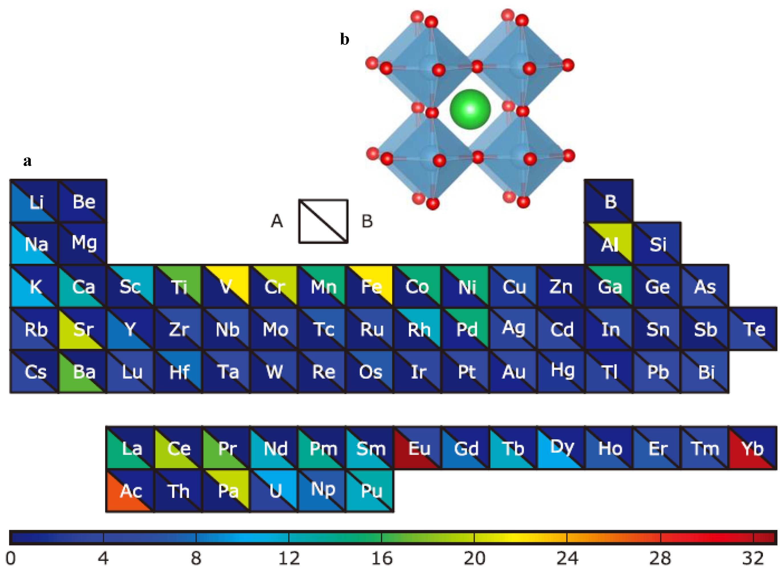
All 21,316 compounds are generated by filling the A and B positions (73² × 4 = 21,316) in the ABX₃ (X = O, Br, Cl, I) perovskite crystal structure with 73 metals or semi-metals in the periodic table (see Figure 1a) [27]. The ideal ABX₃ perovskite crystal structure [28] is composed of an A cation in a 12-coordinate structure located in a cavity composed of octahedrons; and a B cation forms an octahedral coordination with six oxygen ions (see Figure 1b). In addition to the ideal cubic structure, many perovskites undergo local distortions. These distorted perovskites may have a variety of symmetrical structures, including diamond, tetragonal, and orthogonal distortion. In this work, all 21,316 compounds were generated in the ideal cubic structure.

In order to improve the accuracy of the ML model and to screen for perovskites that have never been reported in the literature and cannot be characterized, we propose a transfer learning method [29]. First, we used a descriptor with structural features to train an accurate ML model; then we used the trained ML model to predict the 21,316 perovskites as a label and train the new model through the elemental feature descriptors. Since this data set is much larger, we can train a good prediction model using only generic features. As elemental descriptors only depend on component or stoichiometry information, no structure or other information is needed. Once the accurate general model is trained, it can be used to effectively screen new perovskite materials.

2.1. Materials Dataset Preparation and Features

This study generated 21,316 samples, of which 5329 were from Chris et al. [27] with their stability calculated via high-throughput DFT. We tried to retrieve these 5239 samples from the Material Project (MP) database and obtained 1148 sample data with Crystallographic Information File (CIF) files. Then these samples were divided into two parts (570 and 578, as shown by D1 and D2, respectively), of which the structural features of the 570 samples were calculated by the powerful open source python library Pymatgen [30], and the calculated features and their descriptions are shown in

Table 1. Thirty-one materials features, their descriptions, and descriptions of attributes for D1 dataset CSV file.

Name	Type	Unit	Description
Chemical formula	string	None	Chemical composition of the compound. The first and second elements correspond to the A- and B-site, respectively. The third element is oxygen
Hull distance	number	eV/atom	Hull distance as calculated by the equation of the distortion with the lowest energy. A compound is considered stable if it is within 0.025 eV per atom of the convex hull
Bandgap	number	eV	PBE band gap obtained from the relaxed structure
X_A	number	eV	The electronegativity of the A atom in the compound
X_B	number	eV	The electronegativity of the B atom in the compound
X_O	number	eV	The electronegativity of the O atom in the compound
A_atomic_mass	number	amu	Atomic mass of atom A
B_atomic_mass	number	amu	Atomic mass of atom B
O_atomic_mass	number	amu	Atomic mass of atom O
A_average_ionic_radius	number	ang	The average is taken over all oxidation states of the A element for which data is present
B_average_ionic_radius	number	ang	The average is taken over all oxidation states of the B element for which data is present
O_average_ionic_radius	number	ang	The average is taken over all oxidation states of the O element for which data is present
minDistA	number	None	Atomic distance between the A cation and the nearest oxygen atom
minDistB	number	None	Atomic distance between the B cation and the nearest oxygen atom
A_molar_volume	number	mol	molar volume of A element
B_molar_volume	number	mol	molar volume of B element
O_molar_volume	number	mol	molar volume of O element
A_electrical_resistivity	number	ohmm	electrical resistivity of A element
B_electrical_resistivity	number	ohmm	electrical resistivity of B element
O_electrical_resistivity	number	ohmm	electrical resistivity of O element
A_atomic_radius	number	ang	Atomic radius of element A
B_atomic_radius	number	ang	Atomic radius of element B
O_atomic_radius	number	ang	Atomic radius of element O
LUMO	number	eV	The lowest unoccupied molecular orbital
HOMO	number	eV	The highest occupied molecular orbital
volume	number	Å3	Volumes of crystal structures.
a	number	Å	Lattice parameter a of the relaxed structure
b	number	Å	Lattice parameter b of the relaxed structure
c	number	Å	Lattice parameter c of the relaxed structure
alpha	number	°	α angle of the relaxed structure. α = 90 for the cubic, tetragonal, and orthorhombic distortion
beta	number	°	β angle of the relaxed structure. β = 90 for the cubic, tetragonal, and orthorhombic distortion
gamma	number	°	γ angle of the relaxed structure. γ = 90 for the cubic, tetragonal, and orthorhombic distortion

° degree, the unit of angle.

; the Magpie features of the other 578 samples were calculated by the python library Matminer [31]. The remaining 15,987 samples were generated by replacing the O element with I, Br, and Cl, respectively for all the 5329 ABO₃ from Chris et al. Finally, we combined all the data of ABX₃ (X = O, I, Cl, Br) leading to a total of 21,316 samples and their Magpie features were calculated. This part of the data set, the D3 as described in Figure 2, was used as the final screening candidates for the convolutional neural network (CNN) screening model.

2.1.1. Structural and Elemental Features

Choosing the right input features is a key step in achieving good predictive performance, thus, the so-called feature engineering. For a materials data set, the features should clearly describe that a single given material can be easily distinguished between different materials. In this study, we selected 31 features, including the elemental and structural features of the atomic composition such as electronegativity, atom radius, band gap, etc. The complete characterization is shown in Table 1.

2.1.2. Magpie Features

The Magpie is a set of extensible attributes, created by Chris et al. [32], that can be used for materials with any number of constituent elements. This set of attributes is broad enough to capture a wide variety of physical/chemical properties that can be used to create accurate models of many material prediction problems. These include stoichiometric characteristics (depending on the proportion of elements only), elemental property statistics (atomic number, atomic radius, melting temperature, etc.), electronic structural properties (valence electrons of s, p, d, and f), and ionic compound characteristics.

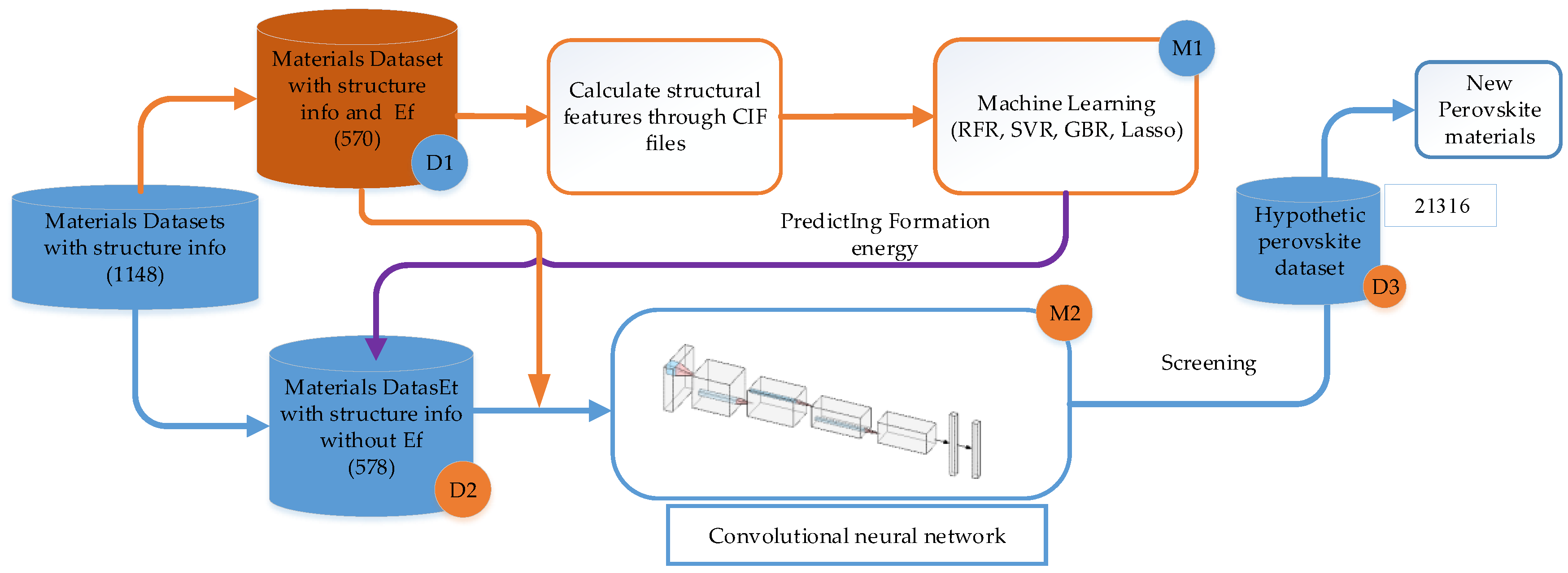
2.2. Overview of Our Data-Driven Framework for Computational Screening

The overall framework of our methodology for screening new perovskites is shown in Figure 2. First, a GBR machine learning model (M1) is trained using the hybrid structural and elemental features and the training dataset D1. The M1 model is then used to predict the formation energies of the materials dataset D2 of which all samples come with structural information. D1 and D2 datasets are then combined to train a convolution neural network model M2 using the elemental magpie features which do not need structural information. This M2 model can then be used to do large-scale screening of candidate dataset D3 to identify potential new perovskite materials for further DFT or experimental verification.

In the following sections, we will describe each step of our screening framework.

2.3. GBR Machine Learning Model for Formation Energy Prediction

It has been shown [33] that training a perovskite specific formation energy prediction model using structural information can achieve high accuracy comparable to that of a DFT calculation. Instead of using artificial neural networks and elemental features only, as done before, we propose to use GBR with both structural and elemental features.

Gradient Boosting Regressor

Boosting is a family of algorithms that can promote weak learners to strong learners, and its performance is significantly better than other basic classifiers. Adding new models to the collection in turn is the main idea for improvement. In each particular iteration, a new, basic learner model is trained by the entire integration error that has been learned so far. Its gradient promotion, like other lifting methods, builds the model in stages and uses arbitrary loss functions. It uses the gradient descent method to solve the minimization problem and generates a predictive model in the form of a set of weak predictive models (usually decision trees). Boosting can be used for both regression and classification problems while this study uses it for regression.

The main architecture of GBR includes three elements: the loss function, the weak learner (for prediction), and the addition model. The main idea of this algorithm is to construct a new basic learner, which is most correlated with the negative gradient of the loss function and is related to the whole. Any loss function can be used. In general, the choice of the loss function depends on the user of the algorithm. So far, there have been various loss functions [34]. The mathematical formula for GBR is as follows:

$$F(x)={\displaystyle {\sum }_{m=1}^M{\gamma }_m}{h}_m(x),$$

(1)

where h_m(x) is a basic function and is often referred to as a weak learner. GBR uses a fixed-size decision tree as a weak learner. Decision trees have the ability to process mixed-type data and the ability to model complex functions. Like other enhancement algorithms, GBR builds the addition model in a step-by-step manner, with the following formula:

$$F_m(x)=F_{m-1}(x)+{\gamma }_m{h}_m(x),$$

(2)

At each stage, the decision tree h_m(x) selects the minimized loss function L, giving the current model F_m−1 and F_m−1(x_i), as follows:

$$F_m(x)=F_{m-1}(x)+\arg \underset{h}{\min }{\displaystyle \sum _{i=1}^{n}L(y_i,F_{m-1}(x_i)-h_m(x))},$$

(3)

The initial model F₀ is determined for a particular problem, and for least square regression, the average of the target values is typically chosen. Given any divisible loss function L, the algorithm starts with the initial model. GBR solves this minimization problem by gradient descent numerical methods. The gradient descent direction is the negative gradient of the loss function on the current model F_m−1 and can be calculated for any divisible loss function. The formula is:

$$F_m(x)=F_{m-1}(x)+{\gamma }_m{\displaystyle \sum _{i=1}^n{\nabla }_{F}L(y_i,F_{m-1}(x_i))},$$

(4)

In the gradient-lifting regression tree, there are multiple hyperparameters. The values of the hyperparameters used in this study are:

• max_depth = 6; n_estimators = 500; min_samles_split = 0.5;
• subsample = 0.7; alpha = 0.1; learning_rate = 0.01; loss = ls

To evaluate the performance of GBR, we also evaluated several mainstream machine learning algorithms as the baselines, including random forest regression (RFR), support vector regression (SVR), and least absolute shrinkage and selection operator (Lasso) with the same dataset using the same set of features.

Random forest regression is also a commonly used algorithm in boosting. It is composed of many decision trees trained on each subsample of the dataset and uses their averages to improve prediction accuracy and control overfitting. The sub-sample size is always the same as the original input sample size, but the samples are drawn with replacement if bootstrap = true (default). It is widely used in statistics, data mining, and machine learning. The hyperparameters in random forest (RF) are max_features and n_estimators, where max_features is the number of features to consider when looking for the best segmentation, and n_estimators is the number of trees in the forest. SVR is a commonly used regression algorithm that uses kernel functions to map data from low-dimensional space to high-dimensional space and then uses the support vectors to fit the hyperplane to the final prediction. The SVR has excellent performance in solving prediction problems with high-dimensional features. However, this advantage is reduced when the feature size is much larger than the number of samples. The main hyperparameters in SVR include C, γ, and epsilon, where C is the penalty parameter of the error term and γ is a parameter attached to the rbf function. The last baseline algorithm, Lasso, is a data dimension reduction method that is applicable not only to linear cases but also to nonlinear cases. The Lasso is based on the penalty method to select the variables of the sample data. By compressing the original coefficients, the original small coefficients are directly compressed to 0, so that the variables corresponding to these coefficients are regarded as non-significant variables. These variables are discarded directly. For ordinary linear models, Lasso usually chooses L1 as the penalty term. In this study, all the above machine learning algorithm models and the 10-fold cross-validation method are implemented using the open-source library Scikit-learn [35].

2.4. Structure Information Enabled Transfer Learning and CNN Based Screening ML Model

2.4.1. Transfer Learning

One of the key obstacles of applying machine learning to materials discovery is the limited training data for the most figure of merit (FOM) properties such as the ion-conductivity, thermal conductivity, and formation energy [26]. Here we propose to use a structural information enabled transfer learning method to train a screening model. The basic idea is to train a formation energy prediction model based on structure and elemental features (model M1 in Figure 2) firstly, which usually has high generalization performance due to the informative structural features. This model is then used to predict the formation energies of a large number of samples in the D2 dataset, of which the samples only have structural information but without formation energy. This formation energy annotation step gives us an enlarged dataset (D1 + D2) with a large number of samples with formation energy values. It is then feasible for us to train a deep learning (CNN) based screening model (M2 in Figure 2) based on the enlarged labeled dataset using the Magpie elemental features only. The independence of M1 on the structural feature here is essential as most hypothetical materials only have composition and/or stoichiometry information without the crystal structure information.

2.4.2. Convolutional Neural Network Model

As one of the most successful deep learning models, the convolutional neural network has a special structure compared to traditional neural network models. With multiple data input channels, it can receive multi-dimensional input data, and the complexity of the network model, which greatly reduces the weight sharing structure, reduces the amount of calculation. The neural unit sharing the weights can use the layer-by-layer feature mapping function to perform multi-level understanding of the input data. A general convolutional neural network consists of an input layer, one or more convolutional layers, one or more sampling/pooling layers, a few fully connected layers, and an output layer.

As the core structure in the convolutional neural network, the convolutional layer uses different scale convolution kernels to traverse the input data in the way of weight sharing and extracts different levels of data features for the same data sample through different parameter distributions. The extracted feature maps of different features are stored in different channels of the convolution network in a feature stacking manner to form a high-dimensional data matrix to be used in the next calculation. The calculation formula of the convolution kernel is as follows:

$$x_k^l={\displaystyle \sum _{j=M_k}{x}_j^{l-1}}{w}_{jk}^l+b_k^l,$$

(5)

In Equation (5), $x_k^l$ represents the kth feature of the lth layer; $x_j^{l-1}$ represents the output of the jth feature of the previous layer; ${\omega }_{jk}^l$ represents the l −1th feature of the layer and the kth feature of the layer of the convolution kernel; $b_k^l$ represents the offset of the kth feature of layer l; $M_k$ is the set of all features output after the convolution operation of layer l − 1 and layer l.

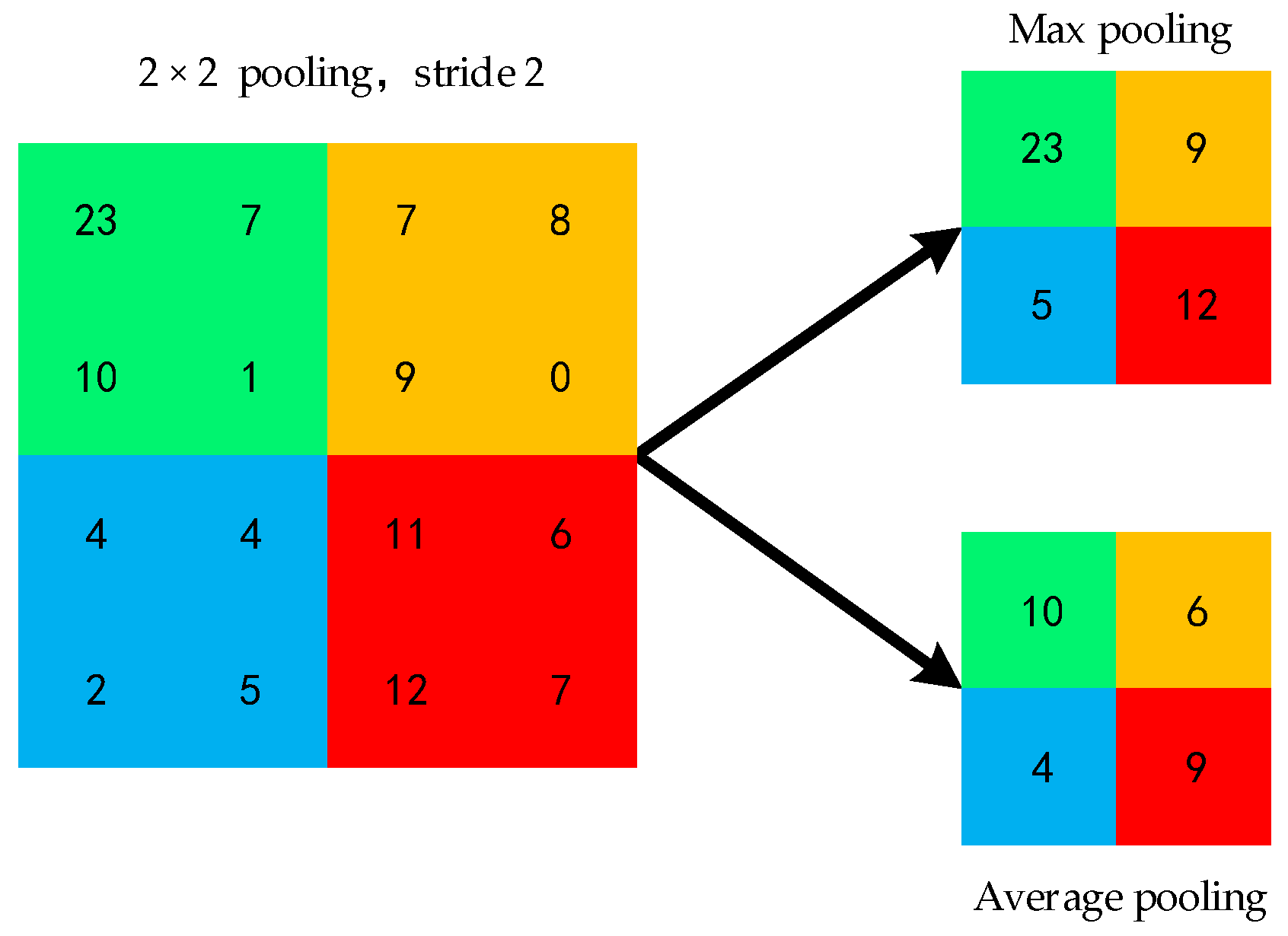
The pooling layer [36] is also called the downsampling layer. After acquiring the features through the convolution layer operation, it is usually useful to use the pooling layer to sample the features calculated by the previous convolution layer to reduce the data dimension and the computational overhead due to the limitation of computing resources and time overhead.

The feature map obtained by calculating the upper convolution layer is divided into non-overlapping rectangular regions, and the operation of taking the maximum value for each rectangular region is called maximum pooling, and the operation of averaging is called averaging pooling. Figure 3 shows the matrix obtained by the maximum pooling and average pooling of the convolutional layer output matrices.

The fully connected layer is located at the end of the convolutional neural network and is a common layer for connecting the output features extracted from the convolutional layers to the prediction output to implement tasks such as classification or regression. All neuron nodes in the fully connected layer are connected to the neuron nodes of the previous layer network, and the high-dimensional data obtained from the previous network layers is tiled as an input. Through the activation function which carries out nonlinear transformation, the fully connected layers learn the mapping of extracted abstract features to predict the desired output

2.4.3. The Convolutional Neural Network Training Process

Training of convolutional neural networks refers to training networks with known samples to learn the mapping between the input and output. It is divided into two stages: forward propagation and backward propagation [37]. Forward propagation refers to the input of the sample into the network, and the output value of the network is obtained by weighting the weight, offset, activation function, and full connection layer parameters of the convolution kernel. Backpropagation first calculates the error between the predicted value of the sample obtained from the forward propagation output and the true value of the sample, and then proceeds backward according to the error value to obtain the error information of each layer, and uses the calculated gradients to adjust the network parameters until the network converges or reaches the specified iteration termination condition.

The forward propagation step feeds the training sample into the network and initializes the parameters of each layer of the network. Through the layer-by-layer calculation of the network, the output corresponding to the input sample under the current network parameters is obtained, that is, a forward propagation is completed. In classification, the output vector characterizes the probability distribution of the sample belonging to the corresponding category, which is calculated by the convolutional neural network. In regression, the output is just a real vector which can be compared with the desired values to calculate the regression loss.

The predicted value of the forward propagation output of the convolutional neural network is compared with the true value and their difference is defined as the loss. Usually for regression, mean square error loss function is used. Then, according to the obtained loss function value, the error value, the parameters of each layer of the network are adjusted and updated to minimize the loss function. The parameters that need to be adjusted in the convolutional network are the weights and offsets of the fully connected layer, and the weights and offsets of the convolutional layer.

For the full layer, the weight and offset of the common network can be solved according to the back propagation algorithm of the common network. The formula is as follows:

$$w_{ij}^l=w_{ij}^l-\eta \frac{\partial }{\partial w_{ij}^l}L,$$

(6)

$$b_i^l=b_i^l-\eta \frac{\partial }{\partial b_i^l}L,$$

(7)

In Equation (6), $w_{ij}^l$ is the weight of the full connection of layer l, $b_{\mathrm{i}}^l$ is the offset of the full connection of layer l, and η is the network learning rate. According to above formulas, the adjustment process of the network parameter is essentially a process of the loss function’s partial derivative of the weight parameter and the offset, and thus the derivation rule can be obtained:

$$\frac{\partial }{\partial w_{ij}^l}L\left(w,b\right)=a_j^l{\delta }_i^{l+1},$$

(8)

$$\frac{\partial }{\partial b_{ij}^l}L\left(w,b\right)={\delta }_i^{l+1},$$

(9)

In Equation (8), $a_j^l$ is the jth neuron input of the lth layer, and ${\delta }_i^{l+1}$ in Equation (9) is the ith neuron error of the l + 1th fully connected layer. Through the above two formulas, the partial derivative of the loss function to the weight and the offset can be obtained, thereby completing the update of the parameters of the fully connected layer network.

The weight update formula of the convolutional layer is similar to that of the fully connected layer. The difference is that the partial derivative value makes a 180° rotation operation based on the output of the previous layer. The partial derivative formula is as follows:

$$\frac{\partial }{\partial w_{ij}^l}L\left(w,b\right)={\delta }_i^{l+1}\ast rot180\left(a_j^l\right),$$

(10)

where $a_j^l$ is the jth neuron input of the lth convolutional layer. ${\delta }_i^{l+1}$ is the ith neuron error of the l + 1th convolutional layer. For the offset parameters of the convolutional layer, the update method is slightly special. This is because in the convolutional layer, the error ${\delta }_i^{l+1}$ is a three-dimensional vector, and the offset $b_i^l$ is a single vector, and the offset update method of the fully connected layer cannot be used. The approach is to sum the respective sub-matrix terms ${\left({\delta }_i^{l+1}\right)}_{u,v}$ of the error ${\delta }_i^{l+1}$ to obtain the error vector, which is the gradient of $b_i^l$, u and v are the height and width of the gradient of the output image when it is reversed. The partial derivative formula is as follows:

$$\frac{\partial }{\partial b_{ij}^l}L\left(w,b\right)={{\displaystyle \sum _{u,v}\left({\delta }_i^{l+1}\right)}}_{u,v},$$

(11)

After the parameters are updated, the training samples will be re-entered into the updated convolutional network model for forward and reverse propagation until the network converges or reaches the specified iteration termination condition, completing the training process.

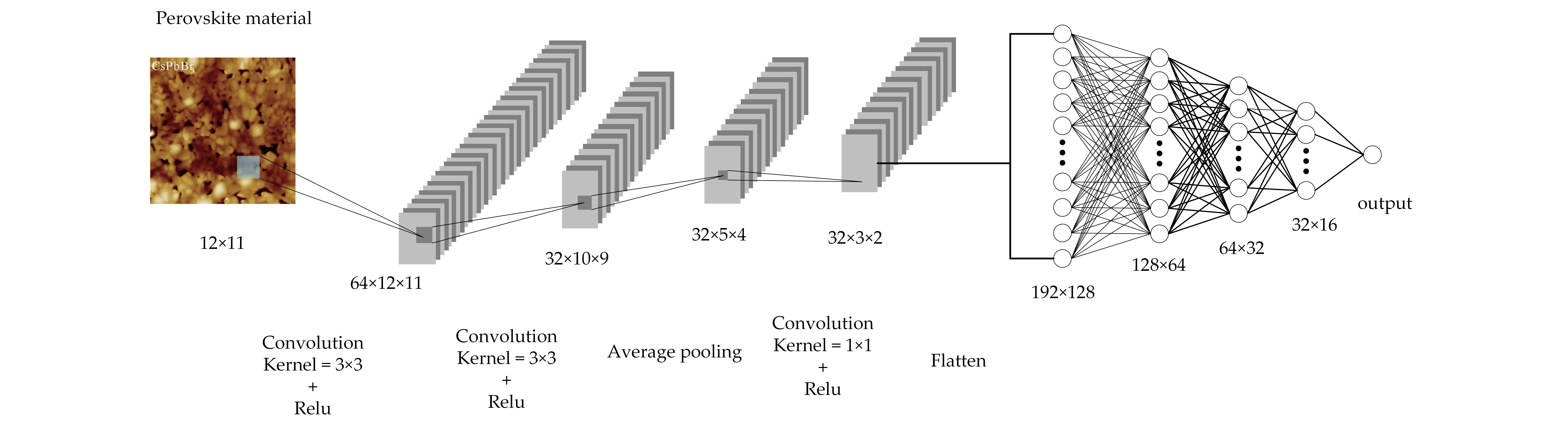
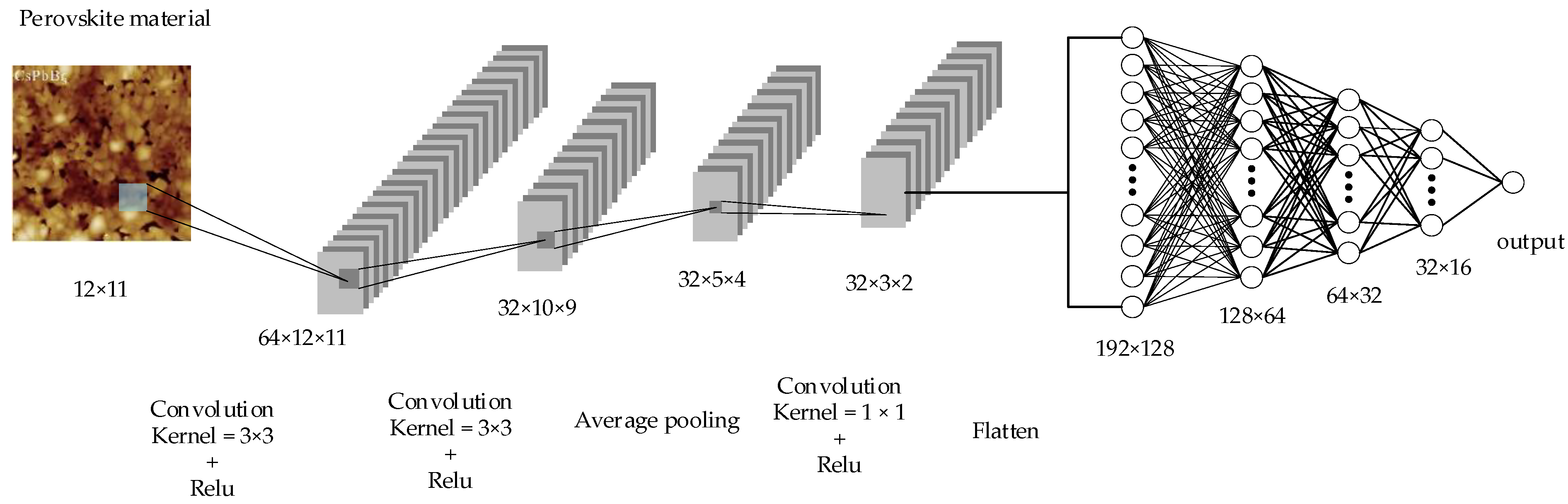
Figure 4 shows our convolutional neural network model for predicting material formation energy. The CNN input is a 12 × 11 fixed size two-dimensional matrix. The structure of the CNN model consists of three convolutional layers and four fully connected layers. The output of the last convolutional layer is expanded into a one-dimensional vector as input to the subsequent fully connected layer. Both the convolutional layer and the fully connected layer use ReLU as the activation function because it is fast, can help address gradient vanishing problem, and can add sparsity to the network. The output of the network is a continuous value, which is the formation energy of the prediction. Our CNN model uses the Adam optimizer and the MAE (mean absolute error) loss function to train the convolutional neural network. The Adam optimizer combines the advantages of multiple optimizers and demonstrates outstanding performance in many applications. In addition, we used 10-fold cross-validation in the assessment and used root mean square error (RMSE), MAE, and R² to evaluate the performance of CNN and other machine learning algorithms.

2.5. Verification Whether a Screened ABX₃ Material is Perovskite or Non-Perovskite

The ABX₃ material after screening by the M2 model is not necessarily a perovskite material. In order to verify whether these ABX₃ candidates are stable perovskites, we use a tolerance factor to predict the stability of the perovskite as proposed by Ghirringhell et al. [38]. It can accurately determine whether the selected ABX₃ material is perovskite or non-perovskite. It only needs chemical composition to predict the stability of perovskite with τ, which makes it possible to verify perovskite materials with unknown structure. In addition to predicting whether the material is a stable perovskite, τ also provides a monotonic estimate of the probability of the material’s stability in the perovskite structure. Its accuracy and probability, as well as its widespread presence in a single perovskite and double perovskite, provide a new physical insight for the stability of perovskite structure. The formula for τ is as follows:

$$\tau =\frac{r_X}{r_B}-n_A(n_A-\frac{\raisebox{1ex}{$r_A$}\!\left/ \!\raisebox{-1ex}{$r_B$}\right.}{In(\raisebox{1ex}{$r_A$}\!\left/ \!\raisebox{-1ex}{$r_B$}\right.)}),$$

(12)

where n_A is the oxidation state of A atom, r_A and r_B are the ionic radii of A and B cations, respectively, r_A > r_B. A key aspect of τ performance is the degree to which the sum of ionic radii estimates the inter-atomic bond distance for a given structure.

3. Results and Discussions

3.1. Selection of the Best Material Features and Analysis of Feature Importance

Features or descriptors are an important part of machine learning models. In general, choosing different feature descriptors will have a great impact on the prediction results. In order to prove that our calculated material descriptors (annotated by Hybrid_descriptors from now on) can be used to predict the formation energy of perovskites, we compare it with the descriptors proposed by Ong et al. [33] (Ong_Descriptors) and the Magpie features. These three feature sets are used to predict the perovskite formation energy on the same algorithm and dataset, using RMSE, MAE, and R² as evaluation indicators, all using 10-fold cross-validation. The results are shown in

Table 2. Comparison of three feature sets for formation energy prediction.

Descriptors	RMSE	MAE	R2
Ong_Descriptors	0.15	0.29	0.78
Magpie	0.11	0.25	0.83
Hybrid_descriptors	0.08	0.20	0.88

RMSE: root mean square error; MAE, mean absolute error.

. Obviously, our feature set is superior over the other two feature descriptors in terms of all three evaluation criteria.

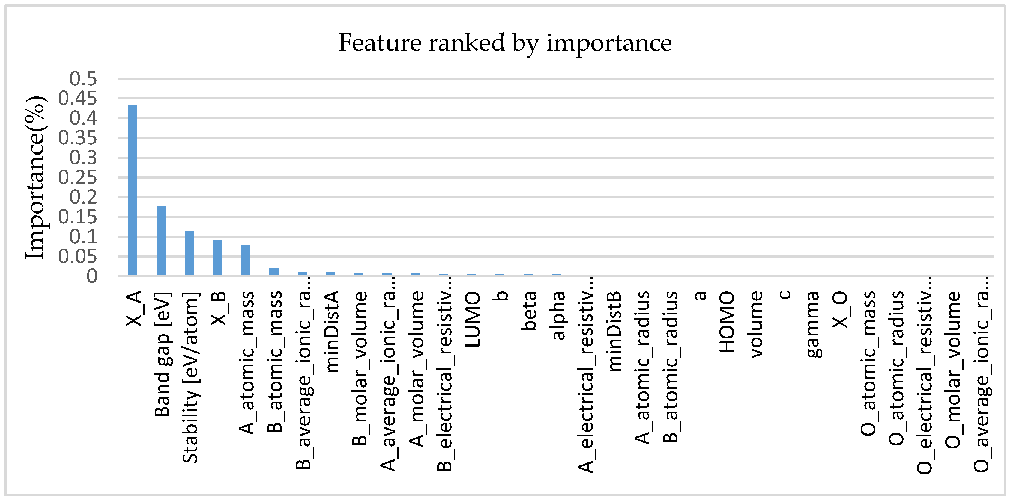
In addition to using a comparative method to validate our proposed feature descriptors, we also analyzed the importance of features using the random forest approach. The random forest consists of a number of decision trees. Every node in the decision trees is a condition on a single feature, designed to split the dataset into two so that similar response values end up in the same set. When training a tree, it can be computed how much each feature decreases the weighted impurity in a tree. For a forest, the impurity decrease from each feature can be averaged and the features are ranked according to this measure. Figure 5 shows the importance scores for all features. It can be seen from the figure that the Pauling electronegativity has a considerable influence on the formation energy of perovskite. It is worth noting that X’s importance score is more than twice higher than the second highest feature, which is consistent with the results of the two literatures [27,39] analyses.

3.2. Performance of the M1 Model with Hybrid Structural and Elemental Features

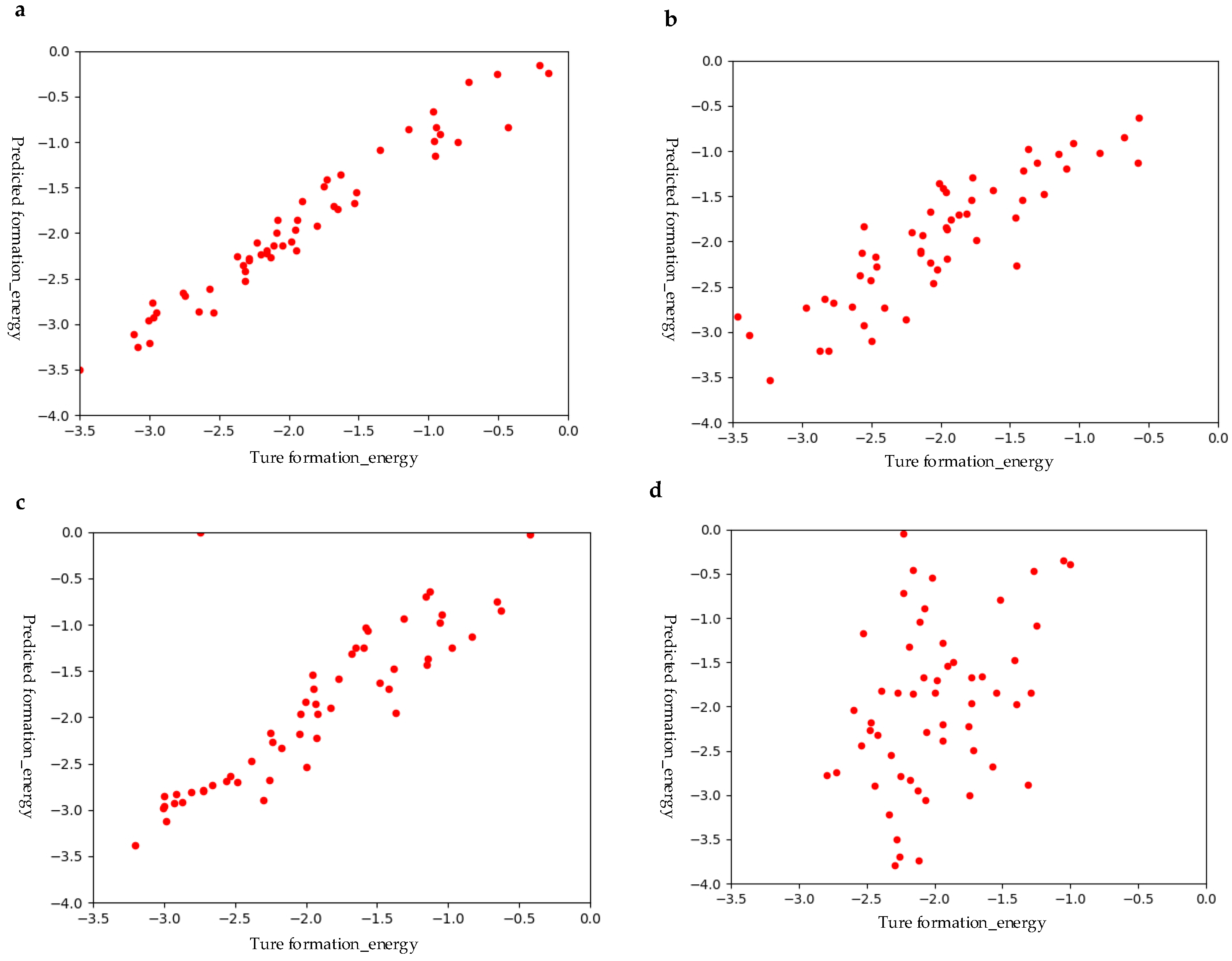
First, we compared the performances of our GBR and other ML models such as RFR, Lasso, and SVR using the hybrid structural and elemental descriptors as raw features. In order to obtain stable results, each algorithm was evaluated using 10-fold cross-validations ten times. Figure 6 shows the fitting accuracy of all models using the same number of samples. It can be clearly seen that GBR has the best prediction performance, followed by RFR, and the worst is SVR. In terms of RMSE, MAE, and R² evaluation criteria, the GBR model scores are 0.28, 0.20, and 0.91, respectively. As shown in

Table 3. RMSE (eV/atom), MAE(eV/atom), and R² values of 10-fold cross-validation results of all prediction models using the hybrid descriptor.

Regression Model	RMSE	MAE	R2
SVR	0.83	0.67	0.20
RFR	0.40	0.29	0.80
Lasso	0.43	0.33	0.75
GBR	0.28	0.20	0.91

, the scores of these three evaluation measures of GBR are the best among all these ML models. In addition to the above three machine learning models, we also tried other machine learning models (such as linear regression models, K-neighbor regression models, etc.) for comparisons. However, their predictions are extremely poor and are therefore not listed here.

The high accuracy of our GBR prediction model can be attributed to the following reasons. One reason is the nonlinear nature of the GBR algorithm; another reason may be the structural similarity of the materials considered in the data set. In a given data set, the crystal structure of all materials is perovskite. Given the same structure, materials with similar chemical compositions may have similar properties, making it more feasible to interpolate properties in predictive models. Discussing structural similarities are beyond the scope of our research, but it has become an important topic in ML research in materials science.

3.3. Performance of M2 Perovskite Screening Model

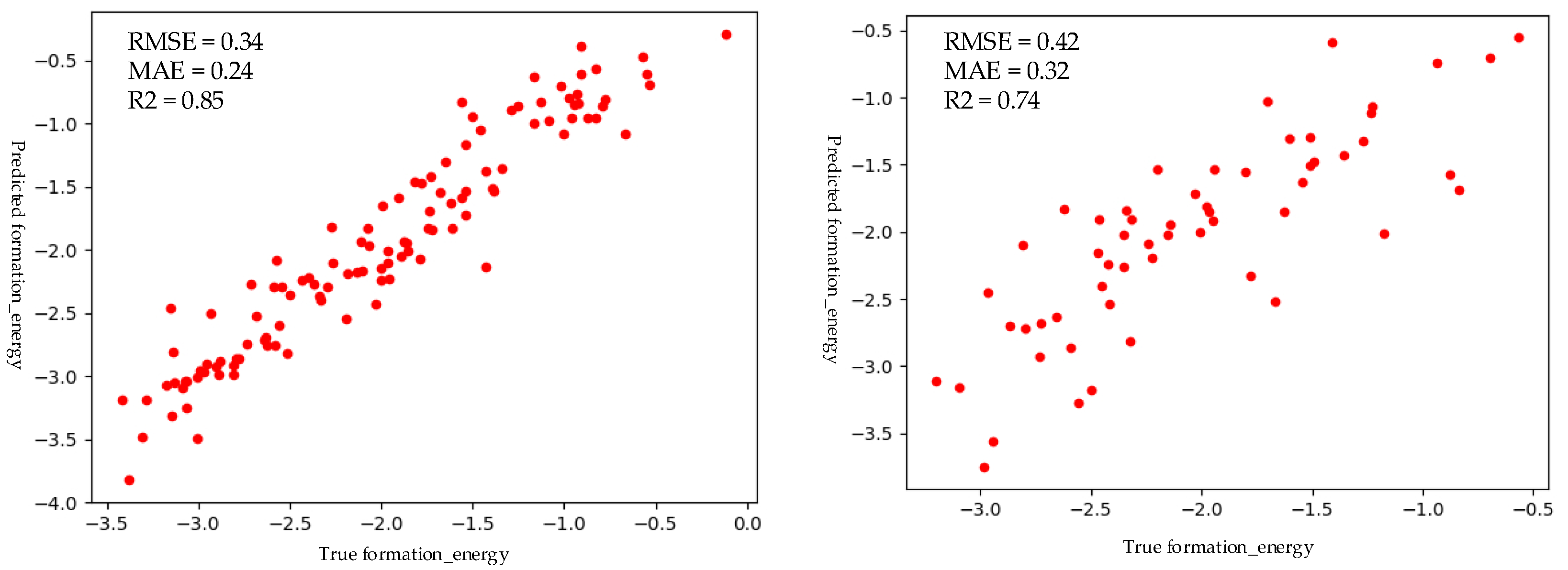
Before we evaluate the performance of the M2 model, a convolutional neural network model, we first compared the prediction performance before and after data enhancement. First, we used the M1 model to label the structured unlabeled D2 dataset and then calculated the Magpie descriptors for datasets D1 and D2. Finally, D1 and D2 datasets were pooled together to predict the perovskite formation energy with M2, and the D1 dataset was used alone to predict the formation energy of the perovskite. It is worth noting here that the labels of the D2 data set are obtained by migrating the learning model M1, and the label of the D1 data set is calculated by the density functional theory (DFT). The results obtained are shown in Figure 7, with the support of the M1 model, the prediction performance has been significantly improved. This also verifies that the hybrid materials features that we proposed play a role.

To further verify that our chosen convolutional neural network model can be used as the best screening model for screening perovskites, we used the ElemNet model proposed by Ward et al. [40], which is a 17-layer deep neural network model, as comparison. The elemental composition is used to predict the formation energy of the material and then screen the material. In addition to using the ElemNet model for comparison, we also compared it to common machine learning models (RF, GBR, SVR, linear regression, K-neighbor regression, etc.), where RF and GBR performed better. As shown in

Table 4. RMSE (eV/atom), MAE (eV/atom), and R² values of cross-validation results of all prediction models using the Magpie descriptor. CNN, convolutional neural network.

Model	RMSE	MAE	R2
ElemNet	0.49	0.64	0.52
RF	0.36	0.27	0.83
GBR	0.35	0.25	0.84
CNN	0.34	0.24	0.85

, we show the results of our convolutional neural network model, the ElemNet model, and the best two traditional machine learning models, the RF and GBR. The results show that our CNN model is the best in terms of RMSE, MAE, and R². Thus, our CNN model is used as the ML model for screening hypothetical perovskites. All of the above models are based on the same data set, and all models have been trained and tested using 10-fold cross-validations.

3.4. Screening Results Analysis

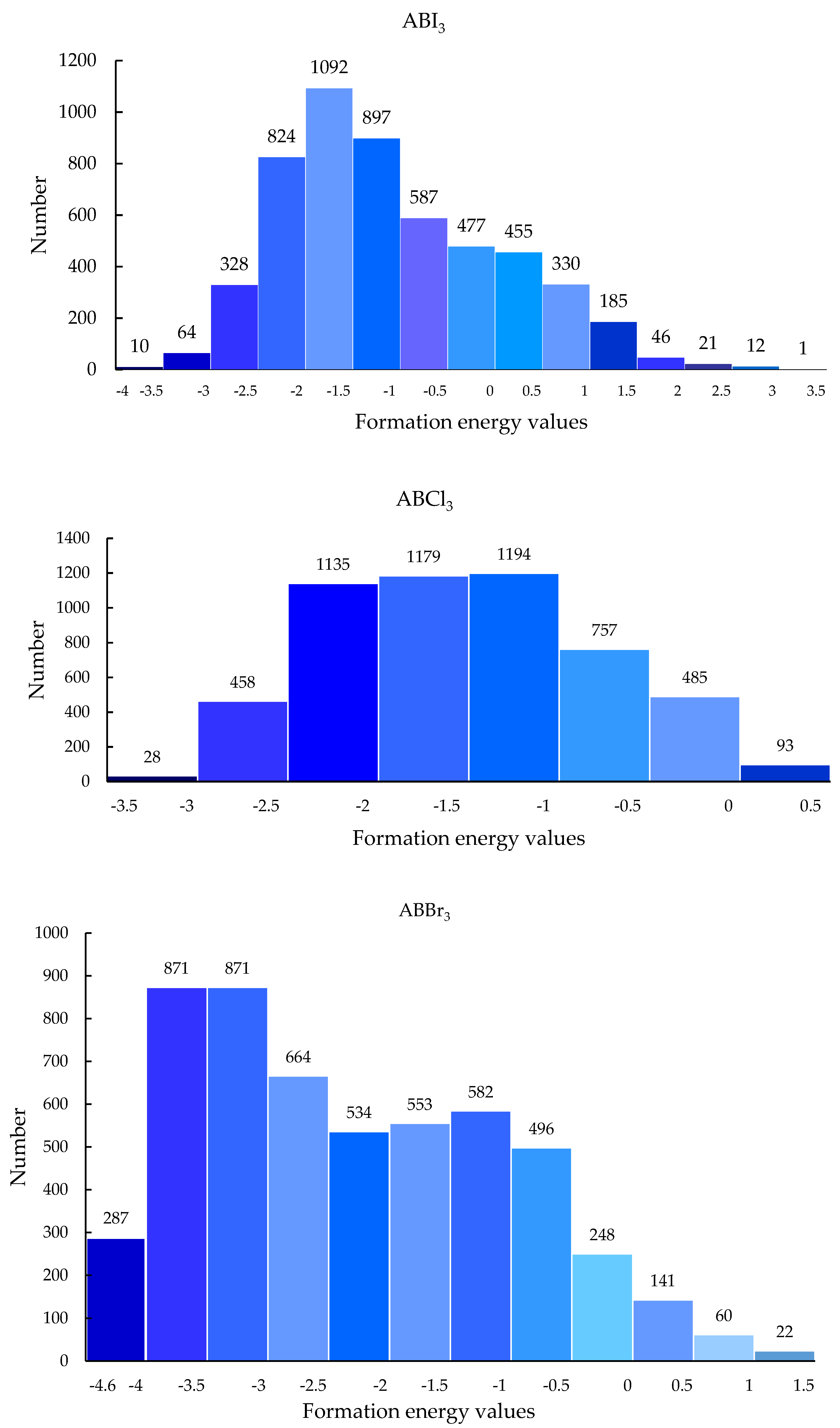
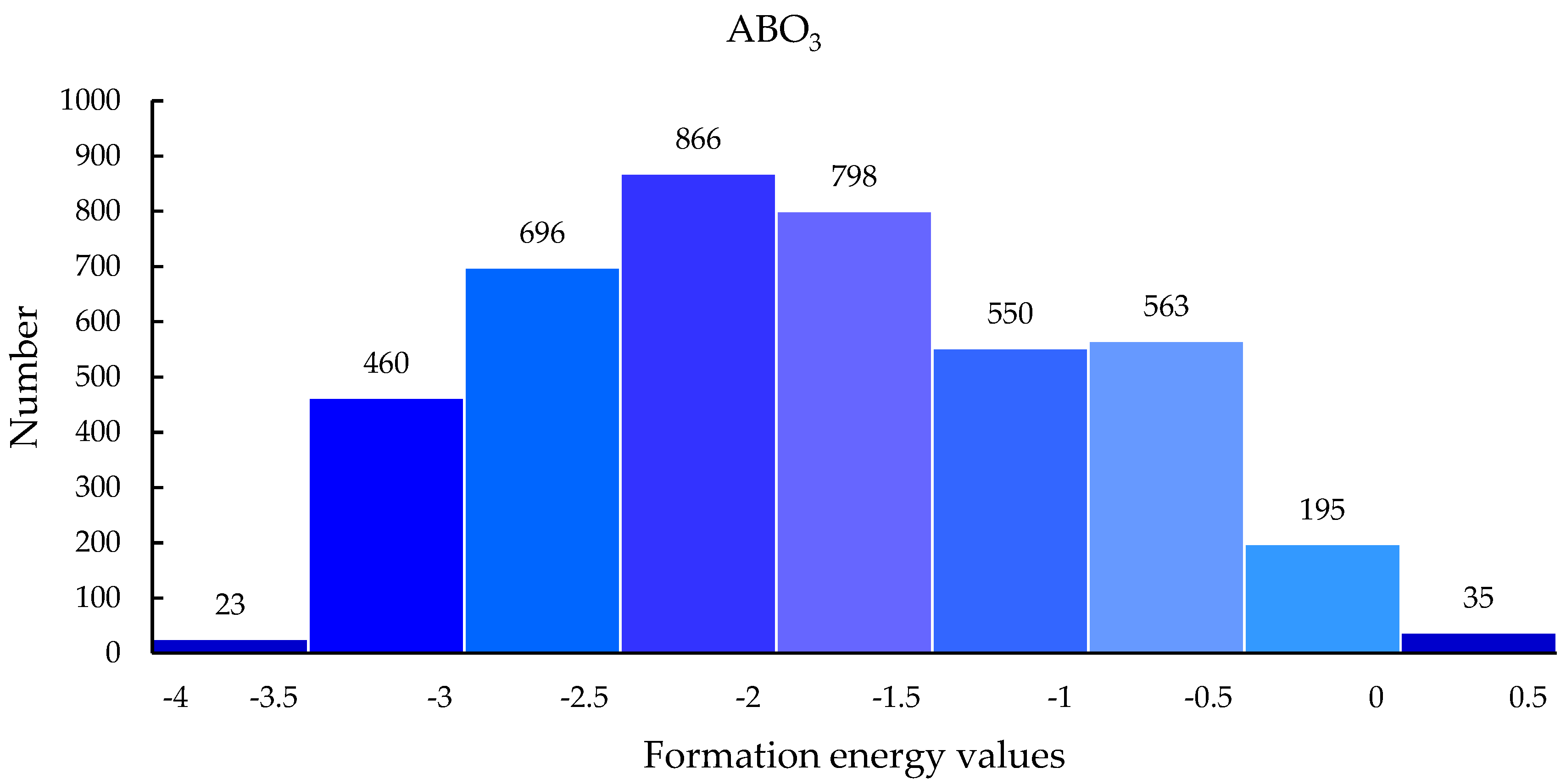
Our CNN model is able to make robust, fast predictions, so it can be used to screen 21,316 materials to discover new and stable perovskite materials. After screening by the M2 model, of 21,316 hypothetical ABO₃ materials, 4147 had formation energy less than 0. More specifically, 5106 were ABBr₃, 5236 were ABCl₃, and 4279 were ABI₃. The specific formation energy prediction value range distribution is shown in Figure 8.

The candidate materials screened out are not necessarily perovskite materials, even though the formation energy may be less than zero. Here we use the new tolerance coefficient τ as discussed before to further screen the selected candidate materials. If the τ of a candidate material is calculated to be less than 4.18, the candidate material has a high probability of being a stable perovskite material. Since τ requires that the ionic radius of the A cation is greater than the ionic radius of the B cation, a portion of the candidate material is therefore filtered out. After screening the new tolerance coefficient τ, there are 625 ABO₃ with τ less than 4.18 along with 52 ABBr₃, 55 ABCl₃, and 32 ABI₃. By reviewing the literature, we found that 98 of the 626 ABO₃s were reported in [27], and 98 perovskites were proved to be stable by DFT calculations. In addition, it was reported [41] that the doped lanthanide BaSnO₃ can be used as the material of the electron transfer layer for a highly efficient and stable solar cell. This material showed up in our screening results. The specific 98 ABO3s are shown in

Table 5. Ninety-eight ABO₃ perovskites calculated by DFT in the literature and our calculated τ value (stability less than 0.025, indicating that ABO₃ perovskite is stable).

Formula	τ	Stability	Formula	τ	Stability	Formula	τ	Stability
NiPtO3	−58.1089	−0.729	RbPuO3	3.4805	−0.103	CeRhO3	1.3071	−0.061
KPaO3	4.0629	−0.567	EuMoO3	3.2674	−0.101	SmVO3	2.9774	−0.057
RbPaO3	3.6251	−0.543	KPuO3	3.78	−0.1	CsNpO3	3.3106	−0.056
LiPaO3	−5.7739	−0.311	SrTcO3	3.8734	−0.097	SmAlO3	1.9819	−0.054
CsPaO3	3.3524	−0.298	BaZrO3	3.7699	−0.096	EuNbO3	4.09	−0.053
BaHfO3	3.7284	−0.247	EuVO3	3.3069	−0.093	BaSnO3	3.6543	−0.052
KNbO3	3.5401	−0.221	AcTiO3	3.8113	−0.092	NpTiO3	3.6701	−0.051
EuGeO3	3.1904	−0.212	CeAlO3	−0.5164	−0.086	KTcO3	3.555	−0.048
EuTcO3	2.8001	−0.15	EuAsO3	2.0406	−0.081	LiOsO3	−2.1229	−0.044
RbNpO3	3.5353	−0.15	CeMnO3	−0.9994	−0.079	CeGaO3	1.8339	−0.043
EuOsO3	−65.0247	−0.143	AcCuO3	3.2679	−0.077	EuIrO3	3.1159	−0.043
KNpO3	3.8902	−0.142	AcNiO3	2.3005	−0.077	GdAlO3	3.1334	−0.041
NpAlO3	−20.7485	−0.129	LaVO3	3.64	−0.077	EuCoO3	3.1653	−0.038
EuRhO3	2.8422	−0.128	PrVO3	3.2155	−0.077	CeNiO3	1.144	−0.037
AcPdO3	3.7105	−0.122	EuAlO3	2.1447	−0.075	YbSiO3	1.9755	−0.032
AcMnO3	1.718	−0.12	AcGaO3	2.4961	−0.073	BaTiO3	3.7351	−0.03
AcFeO3	3.8271	−0.116	LaAlO3	2.3073	−0.072	DyAlO3	2.6055	−0.03
AcVO3	2.6908	−0.116	EuPtO3	3.7879	−0.071	LaGaO3	3.3386	−0.028
EuRuO3	2.0471	−0.112	NdVO3	2.555	−0.071	PuGaO3	−10.427	−0.028
AcAlO3	1.8388	−0.11	EuReO3	2.472	−0.067	YAlO3	3.5597	−0.023
ErAlO3	3.699	−0.022	SrRhO3	3.8864	−0.006	KReO3	3.584	0.008
LaCoO3	3.4776	−0.022	BaPdO3	3.7136	−0.005	YbReO3	3.6451	0.009
NaOsO3	−11.1333	−0.021	KWO3	3.5403	−0.004	CsUO3	3.3037	0.01
PuNiO3	−13.1563	−0.02	BaFeO3	3.7385	0	EuGaO3	3.0439	0.013
LaNiO3	3.0358	−0.019	EuNiO3	2.7795	0	SrCoO3	3.9892	0.014
TmAlO3	2.926	−0.017	LaMnO3	2.1032	0	CeTmO3	−300.872	0.015
SrRuO3	3.6809	−0.013	EuSiO3	1.6849	0.001	DyGaO3	3.8882	0.017
UAlO3	−11.2029	−0.011	NdMnO3	1.6622	0.001	BaPtO3	3.5778	0.019
YbAlO3	3.0372	−0.011	SmMnO3	1.8354	0.001	DyCoO3	4.0617	0.02
SmCoO3	2.8557	−0.009	TbMnO3	0.5464	0.002	YMnO3	3.1268	0.023
SmNiO3	2.5241	−0.009	EuMnO3	1.9694	0.003	DyMnO3	2.3484	0.024
LuAlO3	4.1571	−0.008	SmGaO3	2.7514	0.006	SrIrO3	3.9732	0.025
PuVO3	−7.538	−0.008	NaReO3	4.1088	0.007

. In addition to these 98 compounds, literature [42] proved that one of our predictions, SrMoO₃ in 625 ABO₃, has paramagnetism. Among the 32 ABI₃ screened out by our model, literature [43] verified that CsPbI₃ can be surface-coated with surfactants and environmental conditions are stable. It is expected to be used for light collection or LEDs. Among the 52 ABCl₃ screened out, literature [44] calculated CsPbCl₃ by DFT, and found that the reduction of band gap is due to the limiting effect of carriers, and the increasing number of perovskite layers. Among the 55 ABBr₃ screened out, Anni et al. [45] for the first time reported the temperature dependence of the spontaneous emission (ASE) characteristics of CsPbBr₃ nanocrystalline thin films. Swarnkar et al. [46] verified the luminescence of colloidal CsPbBr₃ perovskite nanocrystals, which surpass traditional quantum dots.

In general, extensive literature inspection shows that our model made reasonable predictions and can be used for discovery of new perovskite materials. The top 200 predicted new perovskites are listed in

Table 6. Top 200 predicted perovskites with predicted τ values (tolerance factor).

Formula	τ	Formula	τ	Formula	τ	Formula	τ
YbTlBr3	−20.162	CaTlCl3	−14.381	CaTlI3	−14.0108	PrBO3	−2.0396
CaTlBr3	−14.3041	NaHgCl3	−13.5492	TlSnI3	2.7082	LiNdO3	−2.0303
CrCoBr3	1.55	MgTlCl3	−6.3625	TlFeI3	2.9924	LiTeO3	−1.945
TlGeBr3	1.6125	TlNiCl3	1.2386	CsCrI3	3.2934	TaBeO3	−1.754
TlFeBr3	2.5339	TlCoCl3	1.4647	CsInI3	3.2934	ThBeO3	−1.7537
CsFeBr3	2.8551	TlGeCl3	1.4794	CsMgI3	3.3089	CeBeO3	−1.7537
CsScBr3	2.8556	TlVCl3	1.5469	CsTiI3	3.3142	CrRhO3	−1.747
CsPdBr3	2.8561	TlCuCl3	1.9923	CsSnI3	3.3312	PuPtO3	−1.6802
CsPtBr3	2.8713	CsPdCl3	2.735	CsGeI3	3.404	ZrBO3	−1.6005
CsInBr3	2.8777	CsSnCl3	2.7368	RbTiI3	3.4157	PrBeO3	−1.5988
CsGeBr3	2.8964	CsCuCl3	2.739	RbSnI3	3.4195	HfBO3	−1.5526
CsNiBr3	2.9272	CsCoCl3	2.7645	CsYbI3	3.4316	TbSiO3	−1.4989
RbCuBr3	2.9466	CsCrCl3	2.7686	CsTmI3	3.4519	SnBO3	−1.4453
RbSnBr3	2.9486	CsInCl3	2.7686	RbVI3	3.4526	CuBO3	−1.3853
RbVBr3	2.9499	BaNiCl3	2.8079	RbCrI3	3.4599	HgRhO3	−1.2912
RbGeBr3	2.9525	RbGeCl3	2.8194	RbInI3	3.4599	GeBO3	−1.0071
RbCoBr3	2.9532	RbCuCl3	2.8216	RbCrI3	3.4599	PaCoO3	−1.0055
RbPdBr3	2.9543	RbSnCl3	2.8251	RbGeI3	3.4601	LiLaO3	−2.8329
RbTiBr3	2.9568	RbPdCl3	2.8331	CsPbI3	3.5094	HgIrO3	−0.9862
CsAuBr3	3.0427	RbFeCl3	2.8369	CsDyI3	3.5292	HgGeO3	−0.9036
RbInBr3	3.0441	RbMgCl3	2.8421	CsCaI3	3.5514	CeAsO3	−0.8
KGeBr3	3.0488	RbScCl3	2.8635	KSnI3	3.5609	TbBeO3	−0.7902
CsYbBr3	3.0711	KCoCl3	2.9149	KTiI3	3.5761	MnSiO3	−0.7002
CsAgBr3	3.0767	KGeCl3	2.9156	CsMnI3	3.6832	CoSiO3	−2.4934
CsCdBr3	3.0839	KVCl3	2.9194	KInI3	3.7193	BiMoO3	−0.2924
ZrSiO3	0.0224	EuMnO3	1.9694	GdBO3	2.2335	TmMnO3	2.6111
ThReO3	0.3455	ThSiO3	−2.1251	GdBeO3	2.2465	PmRuO3	2.6249
NpTaO3	−4.4473	NpSnO3	−2.2195	HoBO3	2.2479	BeAgO3	−4.6185
CuSiO3	0.8738	NdReO3	1.986	YBO3	2.2485	TlSbO3	2.6921
BiRhO3	−2.1807	GdSiO3	2.0075	EuBO3	2.2486	SmGaO3	2.7514
LiSmO3	−2.3252	TlGaO3	2.0255	ErBO3	2.2548	InSiO3	2.7544
TlSiO3	1.5291	LiEuO3	−2.5704	SmBO3	2.2647	LiCdO3	−4.1549
NdBeO3	1.5459	BeAuO3	−4.675	LuBO3	2.2789	BePbO3	−4.5119
AcSiO3	1.5949	PmBeO3	2.0662	AcBO3	2.285	AgAsO3	2.815
ZrBeO3	1.6089	TlWO3	2.0764	VSiO3	-2.9169	AgRuO3	2.8273
SmSiO3	1.6357	ThWO3	2.0875	LiPmO3	-3.731	LiGdO3	−4.5398
SmBeO3	1.6514	TlCoO3	2.0895	LuSiO3	2.3438	SmCoO3	2.8557
LiYbO3	−4.301	TlGeO3	2.1027	TlBO3	2.3453	SmGeO3	2.8773
BeHgO3	−4.2571	BeOsO3	−4.2343	DyMnO3	2.3484	GdAsO3	2.9255
BeCdO3	−4.6077	TmBeO3	2.1393	CrGeO3	2.3535	BeInO3	−5.3548
EuBeO3	1.7345	HoSiO3	2.1444	ThMoO3	2.423	TlFeO3	2.9768
CrWO3	1.7353	LiCaO3	−3.2345	HoBeO3	2.4577	SmVO3	2.9774
LaBeO3	1.8183	BiPtO3	2.145	LiTmO3	−4.0403	LiPrO3	−5.0002
CrTcO3	−2.2119	YSiO3	2.1489	NdGeO3	2.4752	YbAlO3	3.0372
LiCeO3	−4.404	LaAsO3	2.1864	LiDyO3	−3.369	EuGaO3	3.0439
BeBiO3	−4.8111	YbBeO3	2.1968	SmNiO3	2.5241	GaBO3	3.0837
TiBeO3	1.8655	DyBO3	2.2289	ErBeO3	2.535	NdTaO3	3.0888
TlNiO3	1.8873	TmBO3	2.2293	FeAsO3	−3.8096	HgRuO3	−2.1943
TlTcO3	1.898	AgBO3	2.2307	TlCuO3	2.5776	HoMnO3	3.1159
HfBeO3	1.9189	YbBO3	2.2312	LiAcO3	−2.1229	ThBO3	−2.0482

Note: the ABO₃ in this table does not contain the 98 ABO₃ in Table 5. Please check supplementary file for the total 765 predictions.

. The complete set of predicted perovskites is provided in the supplementary file. The remaining non-reported perovskite materials are also promising.

4. Conclusions

In this paper, we proposed to use deep neural network based transfer learning and a hybrid descriptor set for perovskite formation energy prediction. The hybrid descriptors are composed of structural and elemental features as calculated via the pymatgen library. Using these 31 features, our transfer learning algorithm can be used to address the small data issue typical in machine learning based material discovery. It works by first training an annotation model using structured perovskite data sets and then using it to predict the formation energy of unannotated perovskite materials with structures. The experimental results show that the proposed hybrid feature descriptors perform better than the Ong_Descriptors and Magpie descriptors in predicting the perovskite formation energy. Moreover, compared to the commonly used machine learning model, the gradient-enhanced regression that we used outperformed random forest regression, Lasso, and support vector regression models.

Based on the transfer learning method, we established a convolutional neural network perovskite screening model by first labeling unannotated perovskite materials with high-precision structure feature based model and then built a CNN model and trained it with the Magpie descriptors to get a generic screening model, the M2 model, which does not require structural information. Compared to the ElemNet model and several machine learning models, the experiments show that our CNN model is the best in formation energy prediction of perovskites given only composition information. The ABX₃ materials with formation energy greater than 0 were screened out from 21,316 candidates through the CNN model, and the new tolerance factor τ was used to verify whether a screened material is a stable perovskite material. Extensive literature inspection showed that many predicted perovskite materials have been reported in the literature, and the rest is subject to further experimentation or DFT calculation verification.

References

- Aksel, E.; Jones, J.L. Advances in lead-free piezoelectric materials for sensors and actuators. Sensors 2010, 10, 1935–1954. [Google Scholar] [CrossRef] [PubMed]
- Vinila, V.; Jacob, R.; Mony, A.; Nair, H.G.; Issac, S.; Rajan, S.; Nair, A.S.; Satheesh, D.; Isac, J. Ceramic Nanocrystalline Superconductor Gadolinium Barium Copper Oxide (GdBaCuO) at Different Treating Temperatures. J. Cryst. Process Technol. 2014, 4, 168–176. [Google Scholar] [CrossRef] [Green Version]
- Beno, M.; Soderholm, L.; Capone, D.; Hinks, D.; Jorgensen, J.; Grace, J.; Schuller, I.K.; Segre, C.; Zhang, K. Structure of the single-phase high-temperature superconductor YBa2Cu3O7—δ. Appl. Phys. Lett. 1987, 51, 57–59. [Google Scholar] [CrossRef] [Green Version]
- Laffez, P.; Tendeloo, G.V.; Seshadri, R.; Hervieu, M.; Martin, C.; Maignan, A.; Raveau, B. Microstructural and physical properties of layered manganites oxides related to the magnetoresistive perovskites. J. Appl. Phys. 1996, 80, 5850–5856. [Google Scholar] [CrossRef]
- Maignan, A.; Hébert, S.; Pi, L.; Pelloquin, D.; Martin, C.; Michel, C.; Hervieu, M.; Raveau, B. Perovskite manganites and layered cobaltites: Potential materials for thermoelectric applications. Cryst. Eng. 2002, 5, 365–382. [Google Scholar] [CrossRef]
- Song, K.-S.; Kang, S.-K.; Kim, S.D. Preparation and characterization of Ag/MnO x/perovskite catalysts for CO oxidation. Catal. Lett. 1997, 49, 65–68. [Google Scholar] [CrossRef]
- Suntivich, J.; May, K.J.; Gasteiger, H.A.; Goodenough, J.B.; Shao-Horn, Y. A perovskite oxide optimized for oxygen evolution catalysis from molecular orbital principles. Science 2011, 334, 1383–1385. [Google Scholar] [CrossRef]
- Yuan, M.; Quan, L.N.; Comin, R.; Walters, G.; Sabatini, R.; Voznyy, O.; Hoogland, S.; Zhao, Y.; Beauregard, E.M.; Kanjanaboos, P. Perovskite energy funnels for efficient light-emitting diodes. Nat. Nanotechnol. 2016, 11, 872–877. [Google Scholar] [CrossRef]
- Cho, H.; Jeong, S.-H.; Park, M.-H.; Kim, Y.-H.; Wolf, C.; Lee, C.-L.; Heo, J.H.; Sadhanala, A.; Myoung, N.; Yoo, S. Overcoming the electroluminescence efficiency limitations of perovskite light-emitting diodes. Science 2015, 350, 1222–1225. [Google Scholar] [CrossRef]
- Veldhuis, S.A.; Boix, P.P.; Yantara, N.; Li, M.; Sum, T.C.; Mathews, N.; Mhaisalkar, S.G. Perovskite materials for light-emitting diodes and lasers. Adv. Mater. 2016, 28, 6804–6834. [Google Scholar] [CrossRef]
- Kojima, A.; Teshima, K.; Shirai, Y.; Miyasaka, T. Organometal halide perovskites as visible-light sensitizers for photovoltaic cells. J. Am. Chem. Soc. 2009, 131, 6050–6051. [Google Scholar] [CrossRef] [PubMed]
- Kim, H.-S.; Lee, C.-R.; Im, J.-H.; Lee, K.-B.; Moehl, T.; Marchioro, A.; Moon, S.-J.; Humphry-Baker, R.; Yum, J.-H.; Moser, J.E. Lead iodide perovskite sensitized all-solid-state submicron thin film mesoscopic solar cell with efficiency exceeding 9%. Sci. Rep. 2012, 2, 6022–6025. [Google Scholar] [CrossRef] [PubMed] [Green Version]
- Yang, Y.; Ri, K.; Mei, A.; Liu, L.; Hu, M.; Liu, T.; Li, X.; Han, H. The size effect of TiO2 nanoparticles on a printable mesoscopic perovskite solar cell. J. Mater. Chem. A 2015, 3, 9103–9107. [Google Scholar] [CrossRef]
- Yang, W.S.; Park, B.-W.; Jung, E.H.; Jeon, N.J.; Kim, Y.C.; Lee, D.U.; Shin, S.S.; Seo, J.; Kim, E.K.; Noh, J.H. Iodide management in formamidinium-lead-halide—Based perovskite layers for efficient solar cells. Science 2017, 356, 1376–1379. [Google Scholar] [CrossRef] [PubMed] [Green Version]
- Lin, R.; Xiao, K.; Qin, Z.; Han, Q.; Zhang, C.; Wei, M.; Saidaminov, M.I.; Gao, Y.; Xu, J.; Xiao, M. Monolithic all-perovskite tandem solar cells with 24.8% efficiency exploiting comproportionation to suppress Sn (ii) oxidation in precursor ink. Nat. Energy 2019, 4, 864–873. [Google Scholar] [CrossRef]
- Shi, Z.; Jayatissa, A.H. Perovskites-based solar cells: A review of recent progress, materials and processing methods. Materials 2018, 11, 729. [Google Scholar] [CrossRef] [PubMed] [Green Version]
- Ceder, G.; Morgan, D.; Fischer, C.; Tibbetts, K.; Curtarolo, S. Data-mining-driven quantum mechanics for the prediction of structure. MRS Bull. 2006, 31, 981–985. [Google Scholar] [CrossRef] [Green Version]
- Michie, D.; Spiegelhalter, D.J.; Taylor, C. Machine learning. Neural Stat. Classif. 1994, 13, 19–22. [Google Scholar]
- Rajan, K. Materials informatics: The materials “gene” and big data. Annu. Rev. Mater. Res. 2015, 45, 153–169. [Google Scholar] [CrossRef] [Green Version]
- De Luna, P.; Wei, J.; Bengio, Y.; Aspuru-Guzik, A.; Sargent, E. Use machine learning to find energy materials. Nature 2017, 552, 23–27. [Google Scholar] [CrossRef]
- Ferguson, A.L. Machine learning and data science in soft materials engineering. J. Phys. Condens. Matter 2017, 30, 043002. [Google Scholar] [CrossRef] [PubMed]
- Mannodi-Kanakkithodi, A.; Huan, T.D.; Ramprasad, R. Mining materials design rules from data: The example of polymer dielectrics. Chem. Mater. 2017, 29, 9001–9010. [Google Scholar] [CrossRef]
- Saad, Y.; Gao, D.; Ngo, T.; Bobbitt, S.; Chelikowsky, J.R.; Andreoni, W. Data mining for materials: Computational experiments with A B compounds. Phys. Rev. B 2012, 85. [Google Scholar] [CrossRef] [Green Version]
- Seko, A.; Togo, A.; Hayashi, H.; Tsuda, K.; Chaput, L.; Tanaka, I. Prediction of low-thermal-conductivity compounds with first-principles anharmonic lattice-dynamics calculations and Bayesian optimization. Phys. Rev. Lett. 2015, 115. [Google Scholar] [CrossRef]
- Ghiringhelli, L.M.; Vybiral, J.; Levchenko, S.V.; Draxl, C.; Scheffler, M. Big data of materials science: Critical role of the descriptor. Phys. Rev. Lett. 2015, 114. [Google Scholar] [CrossRef] [Green Version]
- Cubuk, E.D.; Sendek, A.D.; Reed, E.J. Screening billions of candidates for solid lithium-ion conductors: A transfer learning approach for small data. J. Chem. Phys. 2019, 150, 214701. [Google Scholar] [CrossRef] [Green Version]
- Emery, A.A.; Wolverton, C. High-throughput dft calculations of formation energy, stability and oxygen vacancy formation energy of abo 3 perovskites. Sci. Data 2017, 4. [Google Scholar] [CrossRef] [Green Version]
- Schmidt, J.; Shi, J.; Borlido, P.; Chen, L.; Botti, S.; Marques, M.A. Predicting the thermodynamic stability of solids combining density functional theory and machine learning. Chem. Mater. 2017, 29, 5090–5103. [Google Scholar] [CrossRef]
- Pan, S.J.; Yang, Q. A survey on transfer learning. IEEE Trans. Knowl. Data Eng. 2009, 22, 1345–1359. [Google Scholar] [CrossRef]
- Ong, S.P.; Richards, W.D.; Jain, A.; Hautier, G.; Kocher, M.; Cholia, S.; Gunter, D.; Chevrier, V.L.; Persson, K.A.; Ceder, G. Python Materials Genomics (pymatgen): A robust, open-source python library for materials analysis. Comput. Mater. Sci. 2013, 68, 314–319. [Google Scholar] [CrossRef] [Green Version]
- Ward, L.; Dunn, A.; Faghaninia, A.; Zimmermann, N.E.; Bajaj, S.; Wang, Q.; Montoya, J.; Chen, J.; Bystrom, K.; Dylla, M. Matminer: An open source toolkit for materials data mining. Comput. Mater. Sci. 2018, 152, 60–69. [Google Scholar] [CrossRef] [Green Version]
- Ward, L.; Agrawal, A.; Choudhary, A.; Wolverton, C. A general-purpose machine learning framework for predicting properties of inorganic materials. npj Comput. Mater. 2016, 2. [Google Scholar] [CrossRef] [Green Version]
- Ye, W.; Chen, C.; Wang, Z.; Chu, I.-H.; Ong, S.P. Deep neural networks for accurate predictions of crystal stability. Nat. Commun. 2018, 9, 3800. [Google Scholar] [CrossRef] [PubMed]
- Bishop, C.M. Pattern Recognition and Machine Learning; Springer: Berlin/Heidelberg, Germany, 2006. [Google Scholar]
- Pedregosa, F.; Varoquaux, G.; Gramfort, A.; Michel, V.; Thirion, B.; Grisel, O.; Blondel, M.; Prettenhofer, P.; Weiss, R.; Dubourg, V. Scikit-learn: Machine learning in Python. J. Mach. Learn. Res. 2011, 12, 2825–2830. [Google Scholar]
- Zeiler, M.D.; Fergus, R. Stochastic pooling for regularization of deep convolutional neural networks. arXiv 2013, arXiv:1301.3557. [Google Scholar]
- LeCun, Y.; Bottou, L.; Bengio, Y.; Haffner, P. Gradient-based learning applied to document recognition. Proc. IEEE 1998, 86, 2278–2324. [Google Scholar] [CrossRef] [Green Version]
- Bartel, C.J.; Sutton, C.; Goldsmith, B.R.; Ouyang, R.; Musgrave, C.B.; Ghiringhelli, L.M.; Scheffler, M. New tolerance factor to predict the stability of perovskite oxides and halides. Sci. Adv. 2019, 5. [Google Scholar] [CrossRef] [Green Version]
- Im, J.; Lee, S.; Ko, T.-W.; Kim, H.W.; Hyon, Y.; Chang, H. Identifying Pb-free perovskites for solar cells by machine learning. npj Comput. Mater. 2019, 5. [Google Scholar] [CrossRef] [Green Version]
- Jha, D.; Ward, L.; Paul, A.; Liao, W.-K.; Choudhary, A.; Wolverton, C.; Agrawal, A. Elemnet: Deep learning the chemistry of materials from only elemental composition. Sci. Rep. 2018, 8, 1–13. [Google Scholar] [CrossRef]
- Shin, S.S.; Yeom, E.J.; Yang, W.S.; Hur, S.; Kim, M.G.; Im, J.; Seo, J.; Noh, J.H.; Seok, S.I. Colloidally prepared La-doped BaSnO3 electrodes for efficient, photostable perovskite solar cells. Science 2017, 356, 167–171. [Google Scholar] [CrossRef]
- Mehmood, S.; Ali, Z.; Khan, I.; Khan, F.; Ahmad, I. First-Principles Study of Perovskite Molybdates AMoO 3 (A= Ca, Sr, Ba). J. Electron. Mater. 2019, 48, 1730–1739. [Google Scholar]
- Swarnkar, A.; Marshall, A.R.; Sanehira, E.M.; Chernomordik, B.D.; Moore, D.T.; Christians, J.A.; Chakrabarti, T.; Luther, J.M. Quantum dot–induced phase stabilization of α-CsPbI3 perovskite for high-efficiency photovoltaics. Science 2016, 354, 92–95. [Google Scholar] [CrossRef] [PubMed] [Green Version]
- Chang, Y.; Park, C.H.; Matsuishi, K. First-principles study of the Structural and the electronic properties of the lead-Halide-based inorganic-organic perovskites (CH~ 3NH~ 3) PbX~ 3 and CsPbX~ 3 (X= Cl, Br, I). J.-Korean Phys. Soc. 2004, 44, 889–893. [Google Scholar]
- Balena, A.; Perulli, A.; Fernandez, M.; De Giorgi, M.L.; Nedelcu, G.; Kovalenko, M.V.; Anni, M. Temperature Dependence of the Amplified Spontaneous Emission from CsPbBr3 Nanocrystal Thin Films. J. Phys. Chem. C 2018, 122, 5813–5819. [Google Scholar] [CrossRef]
- Swarnkar, A.; Chulliyil, R.; Ravi, V.K.; Irfanullah, M.; Chowdhury, A.; Nag, A. Colloidal CsPbBr3 perovskite nanocrystals: Luminescence beyond traditional quantum dots. Angew. Chem. Int. Ed. 2015, 54, 15424–15428. [Google Scholar] [CrossRef]
Figure 1.
(a) is a list of elements considered by the A and B sites. The color coding of the element is a function of the amount of stabilized perovskite and the corresponding element of the A and B positions; (b) is a perovskite structure with 12-fold coordinated A cation (green A atom) and the octahedral coordinated B cation (blue B atom). The X atoms in the three-dimensional (3D) Wyckoff positions are in red.
Figure 2.
Framework for the computational screening of perovskite materials. Abbreviations: RFR, random forest regression; SVR, support vector regression; GBR, gradient boosting regressor; Crystallographic Information File (CIF).
Figure 3.
Pool processing matrix.
Figure 4.
Convolutional neural network architecture for material formation energy prediction.
Figure 5.
Feature importance from random forest (RF) for the formation energy of perovskite.
Figure 6.
Prediction performances of different models using hybrid features: (a) GBR; (b) least absolute shrinkage and selection operator (Lasso); (c) RFR; and (d) SVR.
Figure 7.
Prediction performance comparison of transfer learning model and the baseline model, both using Magpie descriptors. Left: transfer learning model trained with 578 samples labeled by M1 model +570 samples with density functional theory (DFT) formation energies. Right: baseline model trained only with 570 samples with DFT formation energies.
Figure 8.
Formation energy distribution of hypothetical perovskite materials predicted by M2 model.