Effective Assessment of Inelastic Torsional Deformation of Plan-Asymmetric Shear Wall Systems

Abstract

Torsional deformation may occur in plan-asymmetric wall structures during seismic events. In most current seismic design codes, the torsional deformation is handled using the concept of design eccentricity, in which design loads may be excessively amplified. This approach has limitations in accurately estimating the torsional deformation of the plan-asymmetric structures, mainly because it is based on linear elastic material behavior. In this paper, we propose a simple method that can accurately evaluate the inelastic lateral displacement and rotation of plan-asymmetric wall structures and is suitable for use in the displacement-based design method. The effectiveness of the proposed method is verified by comparing its predictions with the results of rigorous time history analyses for a model problem. The comparison shows that the proposed method is able to provide accurate estimates of the inelastic torsional deformation for the plan-asymmetric wall system, while requiring less computational cost than the time history analysis.

1. Introduction

Plan-asymmetric structures may undergo torsional vibration in addition to lateral oscillation if they are subjected to seismic ground motions. This induces an additional internal force, which may lead to excessive deformation in relatively flexible structural components. This excessive deformation often results in the unexpected brittle failure of structures, which has been reported during several earthquake events in the past such as the Mexico earthquake in 1985 [1], the Chile earthquake in 1985 [2], the Loma Prieta earthquake in 1989 [3], and the Kobe earthquake in 1995 [4]. The unsymmetrical distribution of mass and lateral load resisting stiffness of the plan-asymmetric structure is the primary source of the lateral torsional structural response. However, torsional deformation may occasionally be induced even in symmetric structures due to non-uniform ground motions along the foundation of the structure or the inherent torsional components of ground excitation. Details of the structural as well as non-structural members also may be sources of the torsional response.

For this reason, most current seismic design codes include criteria to minimize the torsional response of building structures as well as damage caused by it. The current seismic design codes such as the International Building Code (IBC) [5], New Zealand Standards (NZS) (Standards New Zealand, 2004) [6], the National Building Code of Canada (NBCC) [7] and Eurocode [8] suggest design eccentricity based on the linear elastic state of structural components. However, the inelastic torsional response of a structure is quite different from that in the elastic range. If the main lateral force resisting components begins to yield, the eccentricity, lateral force distribution, and amount of rotation may become quite different from those in the elastic range. Some of the current design code provisions provide a simple solution to this problem by introducing the so-called accidental eccentricity, which is equivalent to the elastic eccentricity amplified by a certain factor. However, this accidental eccentricity may require excessive strength and stiffness for lateral force resisting components since it does not properly consider the actual torsional failure mechanism of the structure.

There has been a lot of research performed to remove the limitations of the current seismic design codes and develop a proper design process. Early stage research on this issue focused on the force-based design approach, which still offers the theoretical basis to most of the current practical design codes. The main issue with this approach was the reasonable determination of design eccentricities. In [9], Goel and Chopra first proposed a design eccentricity based on the inelastic torsional behavior of plan-asymmetric structures by considering two performance levels, i.e., serviceability and ultimate limit states. However, their approach may overestimate the strength of relative flexible wall components. To handle this issue, Duan and Chandler [10] suggested a modified design eccentricity that provides optimal ductility requirements and overstrength factors on both flexible and stiff wall components, but it still may underestimate the design eccentricity at the intermediate inelastic stage. Humar and Kumar [11] investigated the effect of wall components perpendicular to the excitation direction based on concepts similar to those proposed in [9,10].

The displacement-based design approach has also been researched to properly handle this issue. Since the deformation is a better measurement of structural performance than strength or stiffness, most recently proposed design methodologies adopt this approach. In [12,13], Paulay estimated the required system ductility of an asymmetric structure based on its torsional mechanism instead of proposing an effective design eccentricity. De Stefano et al. [14] evaluated the inelastic torsional behavior in terms of strength eccentricity. They showed that the torsional behavior of an asymmetric structure can be minimized if its strength center is located between the stiffness and mass centers. De la Llera and Chopra [15] investigated the inelastic seismic behavior of asymmetric multistory buildings using the concept of story shear and torque histories. Lin and Tsai [16] proposed a two-degrees of freedom analysis model consisting of a single lateral force resisting column and a corresponding rotational spring. Panagiotou et al. suggested an accurate two-dimensional cyclic beam-truss model for reinforced concrete shear walls [17], and it was later extended to a three-dimensional model [18]. Cho et al. [19] proposed a modified three-dimensional capacity spectrum method to efficiently evaluate the seismic behavior of a building structure with asymmetric walls. The application of plan-asymmetric analysis techniques to multi-story building structures was discussed by several researchers [20,21,22] by explicitly considering the nonlinear torsional and higher-order effects. Anagnostopoulos et al. [23] published an excellent review paper on the earthquake induced torsion in buildings by grouping various publications into a number of subtopics.

Considering all these issues, this paper proposes a simple method that can accurately assess the inelastic lateral displacement and rotation of plan-asymmetric wall structures. The relationship between the lateral displacement and rotation is obtained by considering the inelastic behavior of asymmetric structures and is presented and interpreted in the displacement-rotation (D-R) coordinate. This coordinate system is very convenient to understand the inelastic torsional behavior of the asymmetric structure. The validity of the proposed method is investigated by comparing its predictions and inelastic time-history analysis results for a model problem.

The outline of this paper is as follows. Following the introduction, Section 2 introduces and summarizes several current seismic code provisions on the torsional design of plan-asymmetric structures. In Section 3, the generalized form of the inelastic lateral displacement-rotation relationship of the structure is derived by following a step-by-step procedure. In Section 4, the effectiveness of the inelastic torsional response assessment procedure proposed in Section 3 is verified by comparing its results with those of time history analyses. Finally, the summary and concluding remarks are provided in Section 5.

2. Current Code Provisions on Torsional Design of Plan-Asymmetric Structures

In general, most of the current seismic design code provisions are based on the force-based design approach. In this approach, the static eccentricity (e) is defined as the distance between the centers of mass and rigidity and is used to compute the torsional moment acting on a plan-asymmetric structure. Based on this definition, the torsional moment (T) can be computed by

$$T=-Ve,$$

(1)

where V is the lateral force applied to the structure. If more than one lateral force components are applied, the resulting torsional moment can be calculated by

$$T=-{\displaystyle \int \overline{e}}\hspace{0.17em}dV,$$

(2)

where $\overline{e}$ is the eccentricity of each lateral force components. From this relation, the effective eccentricity can be derived as follows:

$$e=-\frac{{\displaystyle \int \overline{e}\hspace{0.17em}dV}}{{\displaystyle \int dV}}$$

(3)

The current seismic design codes such as IBC, Eurocode, NZS and NBCC introduce the concept of the design eccentricity (e_design), which can generally be written in the form of

$$e_{design}=\gamma e+\eta b,$$

(4)

where e is the eccentricity defined as the distance between the center of mass (CM) and the center of rigidity (CR), b is the floor plan length perpendicular to the excitation direction, and γ and η are the coefficients specified in the seismic design codes listed in

Table 1. Design torsional eccentricity coefficients specified in several current seismic design codes.

Design Code	γ	η	Note
IBC	1.0	±0.05	A torsional amplification factor Ax is considered if the diaphragm is not rigid.
NZS	1.0	±0.1	-
NBCC	1.0 ± 0.5	±0.1	-
Eurocode	1.0	0.05	Dynamic effect is considered by introducing an additional eccentricity value.

. In Equation (4), the first term on the right-hand side accounts for the natural torsional effect, and the second term incorporates the accidental torsional effect.

The design eccentricity proposed by IBC can be stated as

$$e_{design}=1.0e\pm 0.05b.$$

(5)

In this case, no dynamic amplification is considered, and the eccentricity by accidental torsion is defined as ±5% of the plan length in the direction perpendicular to the applied lateral force. If the diaphragm is not rigid, and the maximum deformation at the edge of the plan considered exceeds 1.2 times the average deformation, the entire design eccentricity expressed by Equation (5) is multiplied by a torsional amplification factor (A_x) given as

$$A_x=\frac{{\delta }_{\max }}{1.2{\delta }_{avg}}\le 3.$$

(6)

In Equation (6), δ_max is the maximum deformation at the plan edge, and δ_avg is the average value of the deformations measured at both of the plan edges.

NZS suggests a design eccentricity similar to that of IBC, which is expressed by

$$e_{design}=1.0e\pm 0.1b.$$

(7)

It can be noted from Equation (7) that no dynamic effect is considered in NZS and ±10% of the plan length in the direction perpendicular to the applied lateral force is used as the eccentricity by accidental torsion. The design eccentricity suggested in NBCC is similar to that of NZS, but the eccentricity amplification due to dynamic effects is also considered. This suggests that the design force should be computed with the maximum eccentricity value among the four possible combinations calculated by

$$e_{design}=\left(1.0\pm 0.5\right)e\pm 0.1b.$$

(8)

In Eurocode 8, if the lateral stiffness and mass are symmetrically distributed on the plan and the accidental torsion is not considered by a more accurate method, the accidental torsional effect can be accounted for by multiplying the load applied to an individual lateral load resisting element with δ, which is given by

$$\delta =1+0.6\frac{x}{L_e},$$

(9)

where x is the distance between the individual element considered and the center of mass in the perpendicular direction to seismic excitation, and $L_e$ is the distance between the two-outermost lateral load resisting elements measured in the same direction as x.

An alternative approximate method to the one above is presented in the annex of Eurocode 8. To consider the dynamic effect of simultaneous lateral and torsional vibrations, two design eccentricity equations, i.e., (10) and (11), are suggested.

$$e_{\max }=e_0+e_1+e_2,$$

(10)

$$e_{\min }=e_0-e_1.$$

(11)

Here, e₀ is the static eccentricity defined by Equation (3), e₁ the accidental eccentricity corresponding to 5% of the plan length in the direction perpendicular to seismic excitation, and e₂ is the additional eccentricity reflecting the dynamic effect induced by simultaneous lateral and torsional vibrations. The dynamic eccentricity e₂ is determined as the smaller of those computed in Equations (12) and (13).

$$e_2=0.1\left(L+B\right)\sqrt{\frac{10e_0}{L}}\le 0.1\left(L+B\right),$$

(12)

$$e_2=\frac{1}{2e_0}\left[l_s{}^2-e_0{}^2-r^2+\sqrt{{\left(l_s{}^2+e_0{}^2-r^2\right)}^2+4e_0{r}^2}\right],$$

(13)

where L and B represent the plan lengths in the directions perpendicular and parallel to seismic excitation, respectively, r is the ratio of the story torsional and lateral stiffness, and l_s indicates the radius of gyration approximated by

$$l_s=\sqrt{\frac{L^2+B^2}{12}}.$$

(14)

The inelastic deformation and actual failure mechanism of plan-asymmetric structures are not considered in any of the seismic design codes discussed up to this point. As a consequence, they may require excessive strength and stiffness for lateral force resisting components. A three-dimensional modal or dynamic time-history analysis can be performed for a more accurate evaluation. However, this is highly complicated and too time-consuming for practical design purposes. Therefore, it is necessary to develop a simple and accurate method for assessing inelastic torsional deformation of plan-asymmetric wall structures.

3. Inelastic Torsional Response of Plan-Asymmetric Structures

The torsional response of plan-asymmetric structures in the inelastic range becomes quite different from that in the linear elastic range. In the linear elastic range, the rotation of the asymmetric structure increases in proportion to the level of the lateral load applied, but if any of the lateral force resisting walls start to yield, there is change in the overall torsional stiffness of the structure, which leads to a change in the eccentricity value as well. This again affects the torsional moment induced in the asymmetric structure, and thus the rotation of the structure increases in a nonlinear fashion in the inelastic range.

To accurately assess the inelastic torsional response of the structure, we derived the generalized form of the inelastic lateral displacement-rotation relation of the structure by following a step by step procedure, and we represent this relation in the lateral displacement-rotation coordinate system in this section. According to the authors’ knowledge, this coordinate system has never been introduced before and is very convenient to describe the inelastic torsional behavior of the asymmetric structure. In addition, we discuss the effects of transverse wall stiffness on the yielding procedure of asymmetric structures.

3.1. Torsional Response of Asymmetric Structures in the D-R Coordinate System

In this section, the generalized form of the displacement-rotation relation of plan-asymmetric structures is derived by assuming that the structure is in the linear elastic range. From this relation, we can derive the inelastic displacement-rotation relation of plan-asymmetric structures.

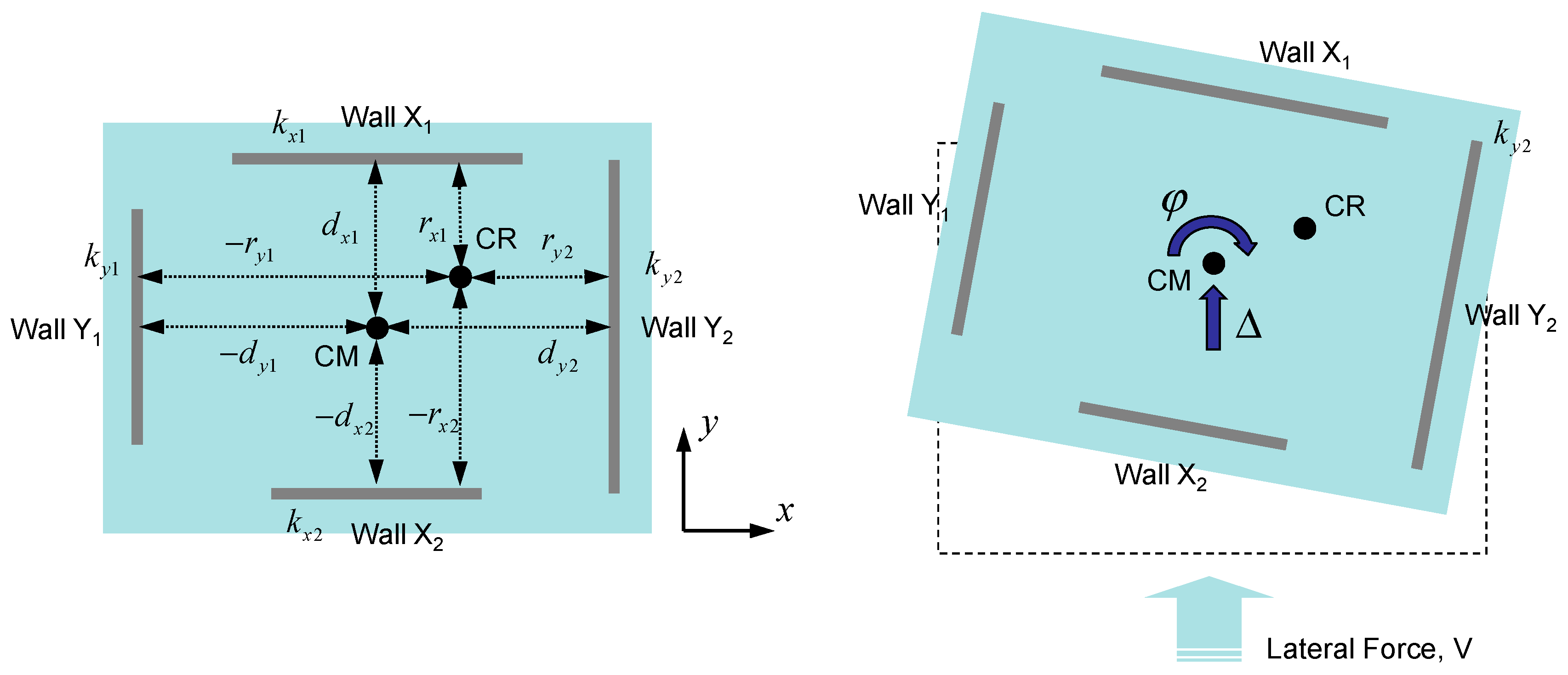
Figure 1 illustrates a representative asymmetric wall structure subjected to a lateral force in the y-direction (V) as well as its deformed shape. In the figure, Wall X_i and Wall Y_i are the i-th lateral load resisting walls in the x- and y-directions, respectively. The x-coordinate of Wall Y_i and y-coordinate of Wall X_i with respect to the center of rigidity (CR) in the undeformed configuration are denoted as r_yi and r_xi, respectively. Similarly, the same quantities with respect to the center of mass (CM) are expressed as d_yi and d_xi, respectively.

The lateral force (V) and torsional moment (T) of the system can be calculated by Equations (15) and (16), respectively:

$$V=K_y\mathsf{\Delta },$$

(15)

$$T=K_T\phi .$$

(16)

Here, K_y and K_T are the lateral stiffness in the y-direction and torsional stiffness of the asymmetric system, respectively. In addition, Δ and ϕ are the lateral displacement and rotation, respectively, and they are estimated at the center of mass. The counterclockwise direction of ϕ is assumed to be positive. In the derivation of Equation (16), we assumed that the diaphragm has an infinite rigidity, and the out-of-plane deformation of the shear wall is ignored. If no external torsional moment is applied, the resulting torsional moment of the asymmetric system can be determined by multiplying the lateral force and the eccentricity in the x-direction between the centers of mass and rigidity (e_x), as given below:

$$T=-V{e}_x.$$

(17)

The eccentricity in the x-direction can be computed by

$$e_x=\frac{{\displaystyle \sum k_{yi}{d}_{yi}}}{{\displaystyle \sum k_{yi}}},$$

(18)

where k_yi is the lateral stiffness of the i-th wall in the y-direction (Wall Y_i).

By substituting Equations (15) and (16) into Equation (17), the rotation can be expressed in terms of the lateral displacement as

$$\phi =-\frac{K_y}{K_T}{e}_x\mathsf{\Delta }.$$

(19)

The lateral and torsional stiffness of the asymmetric structure can be estimated by

$$K_y={\displaystyle \sum k_{yi}},$$

(20)

$$K_T={\displaystyle \sum k_{yi}{r}_{yi}{}^2}+{\displaystyle \sum k_{xi}{r}_{xi}{}^2},$$

(21)

where k_xi represents the lateral stiffness of the i-th wall in the x-direction. By inserting Equations (20) and (21) into Equation (19), the relationship between the lateral displacement and rotation can be obtained as follows:

$$\phi =-\frac{{\displaystyle \sum k_{yi}{d}_{yi}}}{{\displaystyle \sum k_{yi}{r}_{yi}{}^2}+{\displaystyle \sum k_{xi}{r}_{xi}{}^2}}\mathsf{\Delta }.$$

(22)

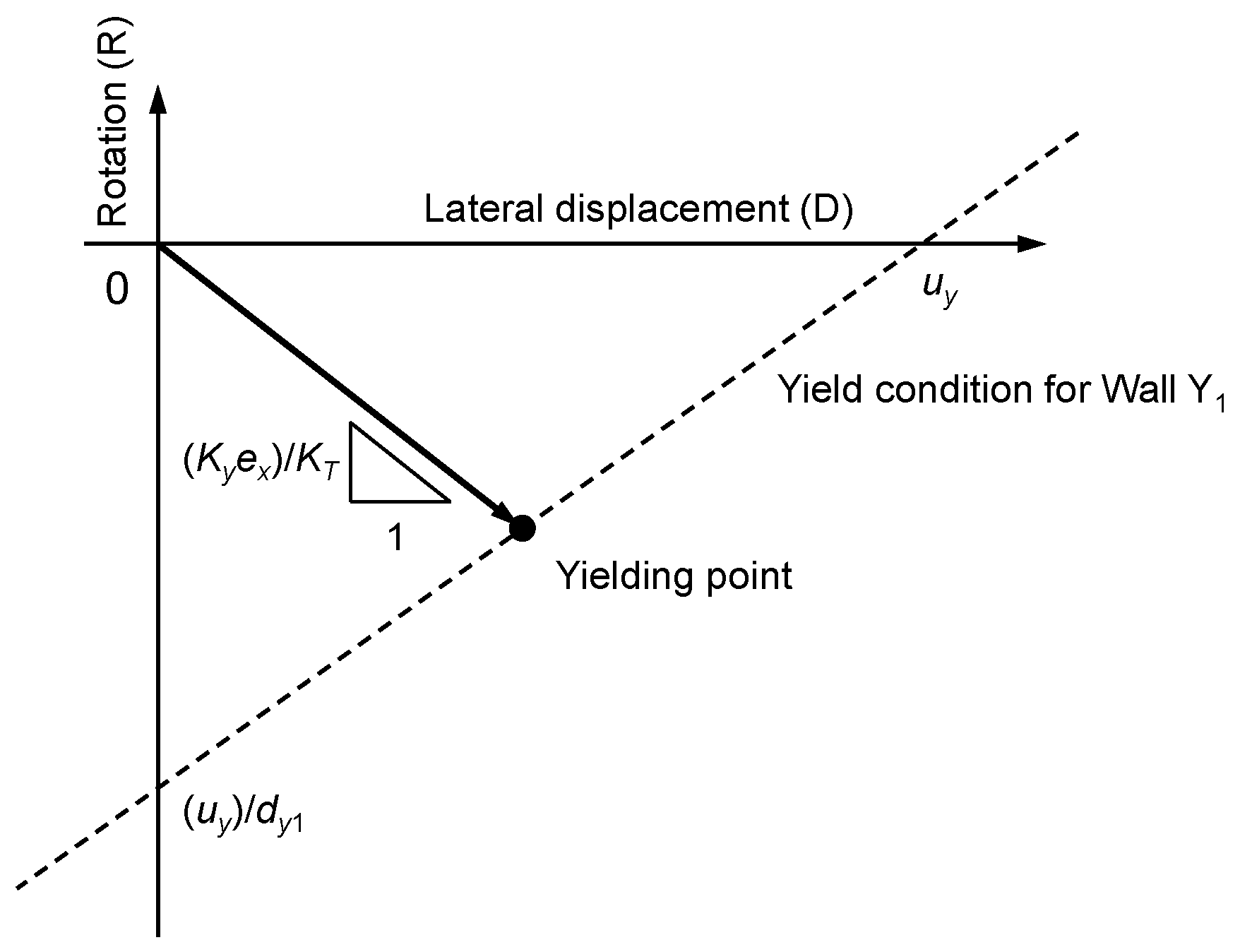
As shown in Figure 2, this relationship can be represented by a solid line with an arrow on the lateral displacement (Δ) and rotation (ϕ) coordinate system, which is denoted as the D-R coordinate system in this paper. This indicates that a linear relation holds between the lateral displacement and the rotation as long as no wall component yields. The yield condition for Wall Y₁ can be stated as

$$\mathsf{\Delta }-d_{y1}\phi =u_y,$$

(23)

where u_y is the yield displacement of Wall Y₁. The figure shows that the yielding of Wall Y₁ occurs at the intersection of Equations (22) and (23). As will be discussed later, this coordinate system is very convenient to describe the inelastic torsional behavior of plan-asymmetric structures.

3.2. Inelastic Torsional Response Assessment Procedure

In this section, we discuss a procedure to assess the inelastic torsional response of plan-asymmetric wall structures. If any wall components yield during the application of lateral force, the linear relationship between the lateral displacement and rotation is no longer valid, and thus it must be modified by considering the reduced stiffness of the wall component that has yielded.

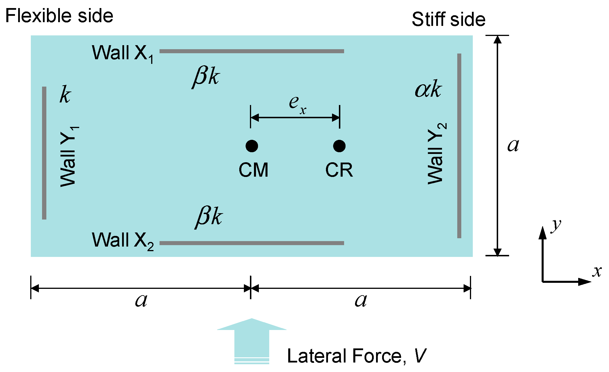
Figure 3 illustrates a simple model problem of plan-asymmetric wall structures to explain the assessment procedure of the inelastic torsional response. This indicates that the structure has two lateral force resisting walls in the x- and y-directions, respectively, and the lateral force is applied in the y-direction. The two walls in the y-direction (Walls Y₁ and Y₂) have elastic lateral stiffnesses of k and αk (α > 1), respectively, and thus Wall Y₂ is stiffer than Wall Y₁. The two walls in the x-direction have the same elastic lateral stiffness βk. Here, β can be of any value, but it may affect the inelastic behavior of the asymmetric structure after yielding of Walls Y₁ and Y₂, as will be discussed later. For simplicity, the out-of-plane deformation of the walls is ignored.

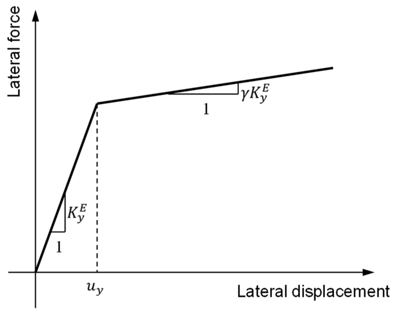
The post yielding behavior of the two lateral force resisting walls Y₁ and Y₂ is defined as a bilinear function, as shown in Figure 4. They have the same yield displacement ($u_y$), and their post-yield stiffness is γ times the elastic stiffness ($K_y^E$). In contrast, we assumed that the other two walls in the transverse direction (Walls X₁ and X₂) remain in the linear elastic range even after the two lateral force resisting walls yield. The inelastic lateral-torsional response of this structure can be obtained by following the step-by-step procedure described below.

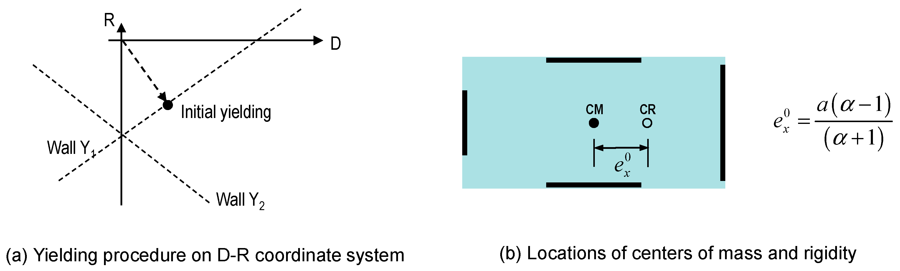
(1) Linear elastic stage

In the linear elastic stage, the lateral displacement and rotation of the asymmetric structure can be computed by Equation (19), where the lateral and torsional stiffnesses and the static eccentricity are estimated by Equations (24)–(26):

$$K_y^0=\left(1+\alpha \right)k,$$

(24)

$$K_T^0=a^2\left(\frac{4\alpha }{\alpha +1}+\frac{\beta }{2}\right)k,$$

(25)

$$e_x^0=\frac{a\left(\alpha -1\right)}{\left(\alpha +1\right)}.$$

(26)

In the above equations, the superscript 0 indicates the linear elastic stage. Finally, Equation (19) can be rewritten as

$${\phi }^0=-\frac{\alpha -1}{a\left(\frac{4\alpha }{\alpha +1}+\frac{\beta }{2}\right)}{\mathsf{\Delta }}^0,$$

(27)

where ${\mathsf{\Delta }}^0$ and ${\phi }^0$ denote the lateral displacement and rotation of the asymmetric structure in the linear elastic stage, respectively.

The deformation history in the displacement-rotation coordinate system and location of the center of rigidity in the linear elastic range are provided in Figure 5. As shown in the figure, the displacement-rotation relationship in the linear elastic stage defined by Equation (27) is represented by a line with an arrow.

(2) First yielding point

As the lateral force increases, the wall on the flexible side yields first since (i) it has greater displacement than the one on the stiff side and (ii) the two walls have the same yield displacement. The wall on the flexible side starts to yield if its y-displacement reaches the yield displacement, and this yield limit can be stated by

$${\mathsf{\Delta }}^0-a{\phi }^0=u_y.$$

(28)

Consequently, the first yielding point can be defined as the intersection of the lines represented by Equations (27) and (28), as shown in Figure 5. This first yielding point (YP₁) can be obtained by inserting Equation (28) into Equation (27), and its coordinates are given by

$$Y{P}_1=\left[{\mathsf{\Delta }}^0,{\phi }^0\right]=\left[\frac{(\beta +8)\alpha +\beta }{2{\alpha }^2+(\beta +8)\alpha +(\beta -2)}{u}_y,-\frac{2\left({\alpha }^2-1\right)}{a\left(2{\alpha }^2+(\beta +8)\alpha +(\beta -2)\right)}{u}_y\right].$$

(29)

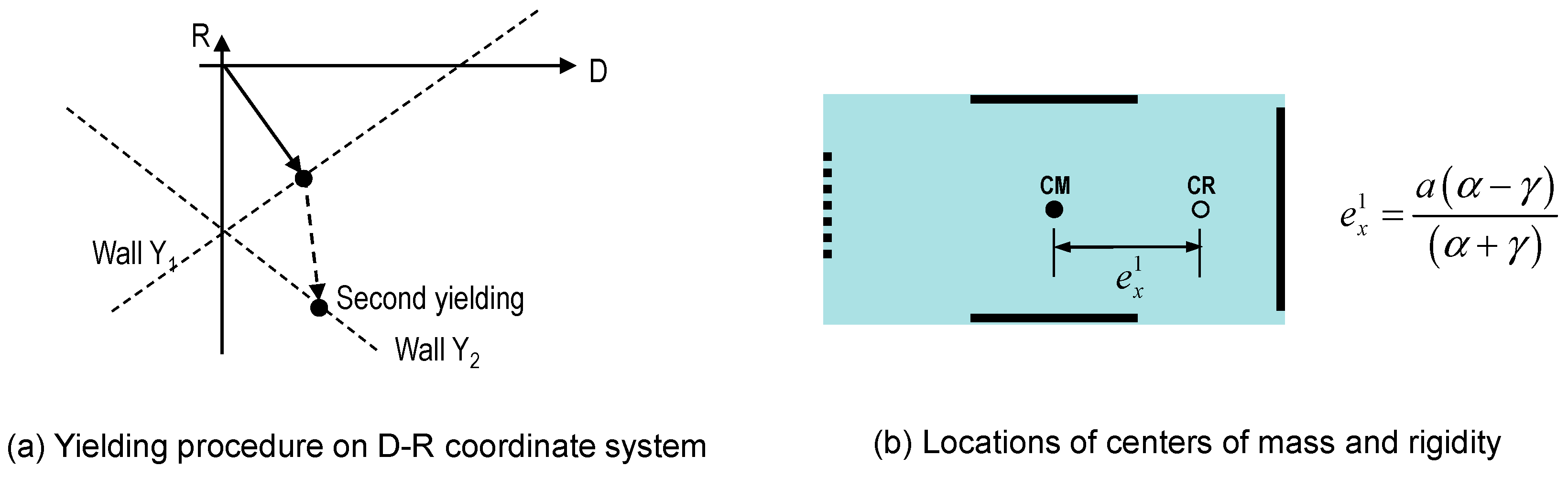
(3) First inelastic stage

After the yielding of the wall component on the flexible side, its lateral stiffness is reduced to γ. From this, the lateral and torsional stiffnesses and the eccentricity of the asymmetric structure can be re-estimated as follows.

$$K_y^1=\left(\gamma +\alpha \right)k,$$

(30)

$$K_T^1=a^2\left(\frac{4\alpha \gamma }{\alpha +\gamma }+\frac{\beta }{2}\right)k,$$

(31)

$$e_x^1=\frac{a\left(\alpha -\gamma \right)}{\left(\alpha +\gamma \right)}.$$

(32)

Here, superscript 1 indicates the first inelastic stage. Similarly, the relationship between the increments of the lateral displacement ($\delta {\mathsf{\Delta }}^1$) and rotation ($\delta {\phi }^1$) after the first yielding can be expressed by

$$\delta {\phi }^1=-\frac{\left(\alpha -\gamma \right)}{a\left(\frac{4\alpha \gamma }{\alpha +\gamma }+\frac{\beta }{2}\right)}\delta {\mathsf{\Delta }}^1.$$

(33)

(4) Second yielding point

A second yielding occurs if the lateral displacement of the wall on the stiff side also reaches the yield displacement with increasing lateral load. This limit state can be expressed by

$$\left({\mathsf{\Delta }}^0+\delta {\mathsf{\Delta }}^1\right)+a\left({\phi }^0+\delta {\phi }^1\right)={\mathsf{\Delta }}^1+a{\phi }^1=u_y.$$

(34)

Like the first yielding, the second yielding point can be obtained by finding the intersection of Equations (33) and (34). This procedure is also illustrated in Figure 6. Thus, $\delta {\mathsf{\Delta }}^1$ and $\delta {\phi }^1$ can be expressed by

$$\delta {\mathsf{\Delta }}^1=\frac{4\left(\alpha (\beta +8\gamma )+\beta \gamma \right)\left({\alpha }^2-1\right)}{\left(-2{\alpha }^2+\alpha (\beta +8\gamma )+(\beta \gamma +2{\gamma }^2)\right)\left(2{\alpha }^2+\alpha (\beta +8\gamma )+(\beta -2)\right)}{u}_y,$$

(35)

$$\delta {\phi }^1=-\frac{8\left({\alpha }^2-{\gamma }^2\right)\left({\alpha }^2-1\right)}{a\left(-2{\alpha }^2+\alpha (\beta +8\gamma )+(\beta \gamma +2{\gamma }^2)\right)\left(2{\alpha }^2+\alpha (\beta +8\gamma )+(\beta -2)\right)}{u}_y.$$

(36)

Finally, the coordinates of the second yielding point (YP₂) can be written as

$$Y{P}_2=Y{P}_1+[\delta {\mathsf{\Delta }}^1,\delta {\phi }^1].$$

(37)

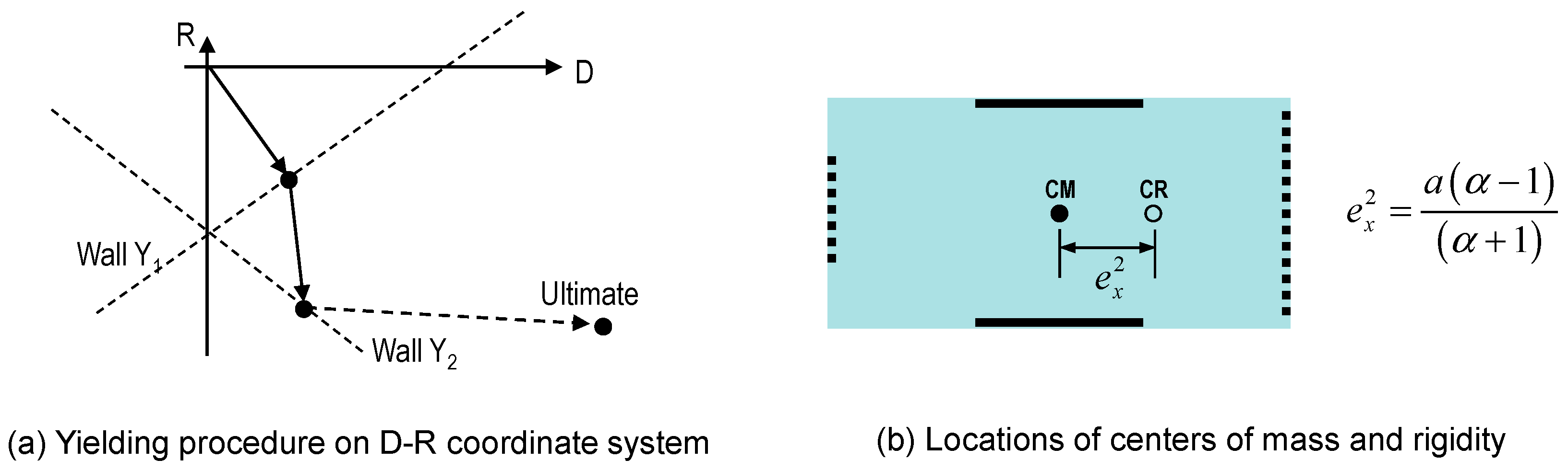
(5) Second inelastic stage (final stage)

As in the case of the wall component on the flexible side, the lateral stiffness of the wall on the stiff side is also reduced to γk. After yielding of the two wall components in the y-direction, the modified lateral and torsional stiffnesses and the eccentricity of the asymmetric system can be respectively expressed by.

$$K_y^2=\gamma k+\alpha \gamma k=\gamma K_y^0,$$

(38)

$$K_T^2=a^2\left(\frac{4\alpha \gamma }{\alpha +1}+\frac{\beta }{2}\right)k,$$

(39)

$$e_x^2=\frac{a\left(\alpha -1\right)}{\left(\alpha +1\right)},$$

(40)

where the superscript 2 indicates the second inelastic stage. Note that the eccentricity in these equations is the same as the one in the linear elastic stage. This is mainly because the lateral stiffnesses of the two walls in the y-direction are assumed to be reduced by the same rate after yielding and the transverse wall components in the x-direction do not contribute to the x-directional stiffness eccentricity. The transverse walls in the x-direction still remain in the elastic stage and now offer relatively large torsional stiffness compared to the wall components in the y-direction. Finally, the relationship between the increase in lateral displacement ($\delta {\mathsf{\Delta }}^2$) and rotation ($\delta {\phi }^2$) at this stage can be given by

$$\delta {\phi }^2=-\frac{\gamma \left(\alpha -1\right)}{a\left(\frac{4\alpha \gamma }{\alpha +1}+\frac{\beta }{2}\right)}\delta {\mathsf{\Delta }}^2,$$

(41)

and this is plotted in Figure 7.

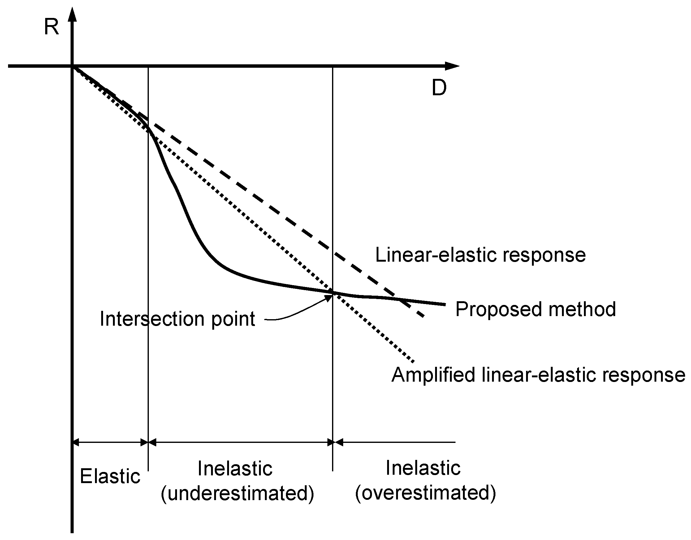
Figure 8 schematically shows the typical lateral-torsional responses of asymmetric structures obtained using three different approaches on the D-R coordinate system based on the discussion up to this point. In the figure, the dashed line represents the linear elastic torsional response given by Equation (22), and the dotted line is the amplified linear elastic torsional response, which is adopted in most of the current design codes in terms of the amplified design eccentricity, as already discussed in Section 2. The solid line represents the inelastic torsional response based on the procedure presented in this section. A comparison of these three curves shows that the amplified linear-elastic response, which is adopted in most of the current design codes, may both underestimate the torsional rotation at the initial yielding stage and overestimate it at the post yielding stage, resulting in an inaccurate estimation of the torsional response over the entire inelastic range.

3.3. Effect of Transverse Wall Stiffness on Yielding Procedure

In the derivation introduced in Section 3.2, we assumed for simplicity that the two lateral force resisting walls have the same yield displacement. As a result, the wall on the flexible side always yields first, and then the wall on the stiff side. However, wall stiffness and yield displacement are determined mainly by the length of the wall. According to [24,25], the stiffness (k) and yield displacement (u_y) of the lateral force resisting wall can be determined by the following two relationships:

$$k\propto l_w{}^3,$$

(42)

$$u_y\propto 1/l_w,$$

(43)

where l_w denotes the wall length. In this case, the stiffness of the transverse wall may affect the overall yielding procedure of asymmetric structures, and this issue is further discussed in this section.

An example problem illustrated in Figure 9 is considered to explore this issue. This is similar to the model problem shown in Figure 3 except that its floor plan has a square shape, not a rectangular shape. The lateral stiffness (k_w1), wall length (l_w1) and yield displacement (u_y,w1) of the flexible side wall Y₁ are denoted by k, l_w and u_y, respectively. The same quantities for the stiff side wall Y₂ (k_w2, l_w2 and u_y,w2, respectively) are given by

$$k_{w2}=\alpha k,$$

(44)

$$l_{w2}=\sqrt[3]{\alpha }{l}_w,$$

(45)

$$u_{y,w2}=u_y/\sqrt[3]{\alpha },$$

(46)

where α is greater than 1 and is the stiffness ratio of the stiff and flexible side walls. Note that the parameters given by Equations (44)–(46) satisfy the conditions stated by (42) and (43). We assumed that the two transverse walls in the x-direction (Walls X₁ and X₂) have the same elastic lateral stiffness as βk and never yield.

By using Equations (18)–(21), the relationship between lateral displacement and rotation angle of the example problem can be expressed by

$$\phi =-\frac{K_Y}{K_T}{e}_x\mathsf{\Delta }=-\frac{\left(\alpha -1\right)}{a\left(\frac{4\alpha }{\alpha +1}+2\beta \right)}\mathsf{\Delta }.$$

(47)

From this equation, the displacement of the two lateral force resisting walls can be derived as

$$u_{w1}=\mathsf{\Delta }-d\phi =\frac{{\alpha }^2+\alpha \left(2\beta +4\right)+\left(2\beta -1\right)}{\alpha \left(2\beta +4\right)+2\beta }\mathsf{\Delta },$$

(48)

$$u_{w2}=\mathsf{\Delta }+d\phi =\frac{-{\alpha }^2+\alpha \left(2\beta +4\right)+\left(2\beta +1\right)}{\alpha \left(2\beta +4\right)+2\beta }\mathsf{\Delta }.$$

(49)

The flexible side wall yields first if the following condition is met:

$$\frac{u_{w1}}{u_{y,w1}}\ge \frac{u_{w2}}{u_{y,w2}}.$$

(50)

By substituting Equations (48) and (49) into Equation (50), we obtain

$$\beta \le \frac{{\alpha }^2\left(\sqrt[3]{\alpha }+1\right)-4\left(\sqrt[3]{\alpha }-1\right)\alpha -\left(\sqrt[3]{\alpha }+1\right)}{2\left(\alpha +1\right)\left(\sqrt[3]{\alpha }-1\right)},\left(\alpha >1\right).$$

(51)

The condition stated by Equation (51) is plotted in Figure 10. The horizontal and vertical axes of the figure represent the total wall stiffness in the excitation and transverse directions, respectively. The results in the figure indicate that first yielding may occur even in the stiff side wall if the total transverse wall stiffness is located in the region above the curve plotted in the figure. For this reason, some researchers have classified plan-asymmetric structures into torsionally unrestrained (TU) and torsionally restrained (TR) structures to consider this effect [11,12,13]. The inelastic torsional response assessment procedure proposed in this study can properly handle this effect without introducing the classification as in the previous research, but none of the current code provisions like IBC and Eurocode consider this effect.

4. Comparison between Predictions by the Proposed Method and Time History Analysis Results

The effectiveness of the inelastic torsional response assessment procedure proposed in Section 3 was verified by comparing its results with those of time history analyses. The proposed method was implemented using the well-known script language MATLAB [26]. The time history analyses were performed by using well-known seismic analysis software, OPENSEES [27], and their solutions are taken as the reference solution.

4.1. Model Problem and Analysis Method

The model problem for verification of the proposed method is the same as the one illustrated in Figure 3. In the model problem, the size of the plan is given as a = 5 m, and the lateral stiffness of Wall Y₁ on the flexible side is taken as k = 1000 kN/m. We assumed that a mass of 500 kg is lumped at the center of mass and the yield displacement of the two lateral force resisting walls in the y-direction is defined as $u_y=0.05\mathrm{m}$. In contrast, we also assumed that the two x-directional walls never yield. A Rayleigh damping ratio of 5% was adopted.

For the time history analysis, each structural wall in the asymmetric structure was modeled using the equivalent truss members, as illustrated in Figure 11. In the modeling, we assumed that the horizontal and vertical trusses are rigid, and the diagonal truss members have zero compressive stiffness (tension only element) to effectively define the hysteretic behavior of the wall component. The elastic stiffness (k_diag) and yield force (P_y,diag) of the diagonal truss elements are defined as follows:

$$k_{diag}=\frac{P_{sys}}{{\mathsf{\Delta }}_{sys}}\frac{d^2+h^2}{d^2}=k_{wall}\frac{d^2+h^2}{d^2},$$

(52)

$$P_{y,diag}=P_{y,wall}\frac{\sqrt{d^2+h^2}}{d},$$

(53)

where k_wall is the elastic lateral stiffness of the wall considered, P_y,wall is its yield force. In addition, P_sys and Δ_sys are the applied lateral force and the lateral displacement at the top of the wall, respectively. Each diagonal truss member consists of two parallel elements, as shown in Figure 12. The primary element among the two elements has an elastic-fully plastic behavior, and the values corresponding to 94% of the total wall yield force and elastic stiffness were set to its yield force and elastic lateral stiffness, respectively. The material behavior of the secondary element is modeled by a fully elastic relationship, of which the elastic stiffness is the 6% of the total wall stiffness. As a result, the structural wall with this diagonal truss member can exhibit the combined bilinear behavior shown in the figure, where the yield force and tangent stiffness after yielding are set to P_y,diag and 0.06k_diag, respectively.

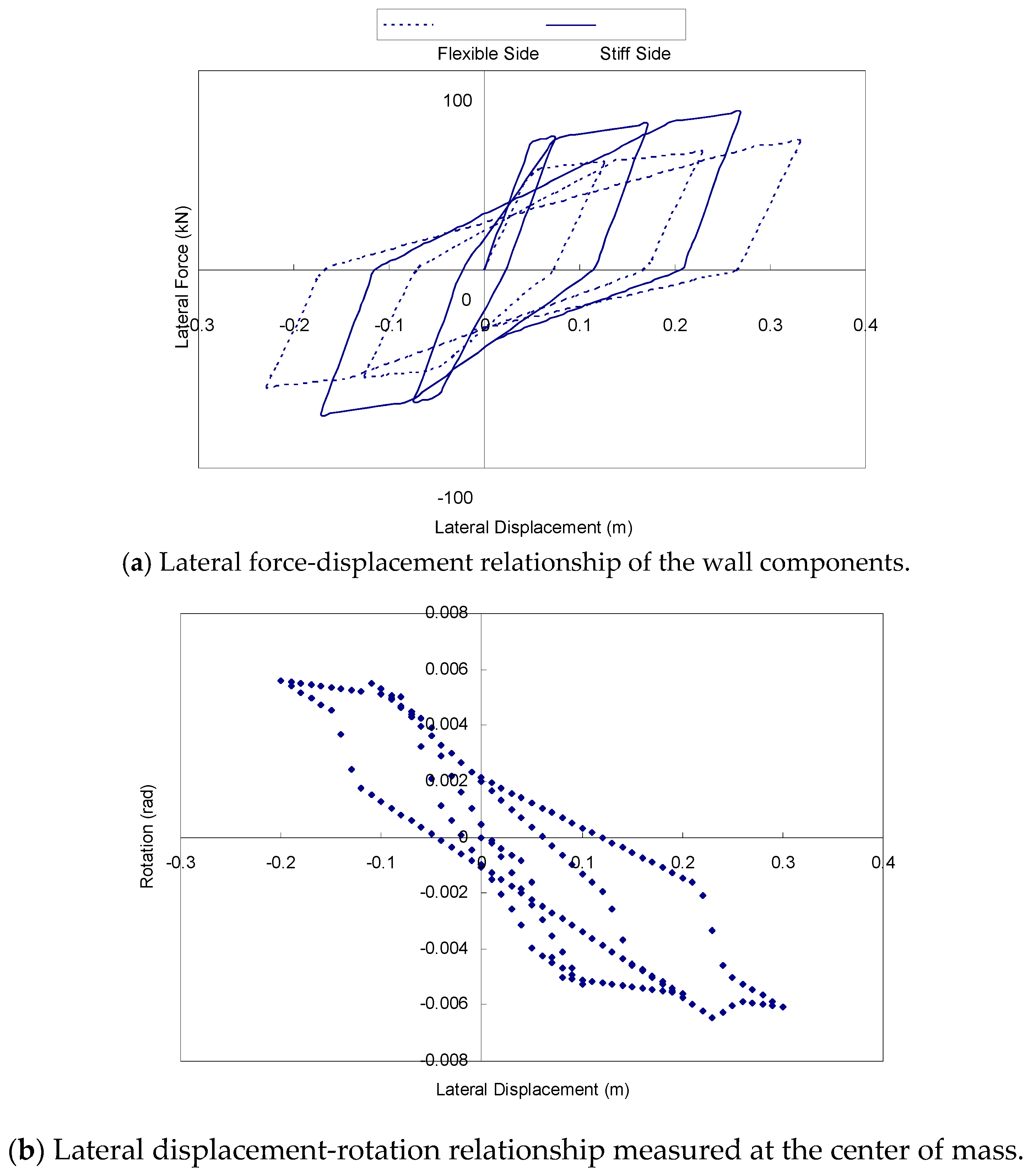
The modified Takeda model was used for the nonlinear hysteretic relationship between the time history analysis because its effectiveness has been verified by numerous experimental results. [28,29] Figure 13 shows the hysteretic response of the model problem when subjected to static cyclic loading. Figure 13a plots the lateral force-displacement relationships for the flexible side wall Y₁ and stiff side wall Y₂, which are distinguished by dotted and solid lines, respectively. Similarly, the relationship between the lateral displacement and rotation angle of the model problem estimated at its center of mass is plotted in Figure 13b.

4.2. Analysis Parameters

This section discusses various parameters that are considered in the time history analysis. As given in

Table 2. Parameters considered in the time history analysis.

α	β	Excitation Data
1.3	0.5 (torsionally unrestrained)	El Centro, Kobe, Northridge, Chichi, Loma Prieta, Parkfield, Turkey
1.6	1.0
2.0	2.0 (torsionally restrained)

, the time history analyses were performed by changing three different types of parameters, which are the relative stiffness of the stiff side wall (α), the relative stiffness of the x-directional (or transverse directional) walls (β), and seismic excitation data applied to the model problem. Three different values (1.3, 1.6 and 2.0) were considered for α, and result in three elastic eccentricity values of the plan-asymmetric model problem, which are 0.65 m, 1.15 m and 1.67 m, respectively. Three values (i.e., 0.5, 1.0 and 2.0) were selected for β and can be categorized as torsionally unrestrained, normal, and torsionally restrained cases, respectively. Seven historical seismic records were selected as input ground excitations for the model problem. Time history analyses were performed for 63 total combinations of the test parameters.

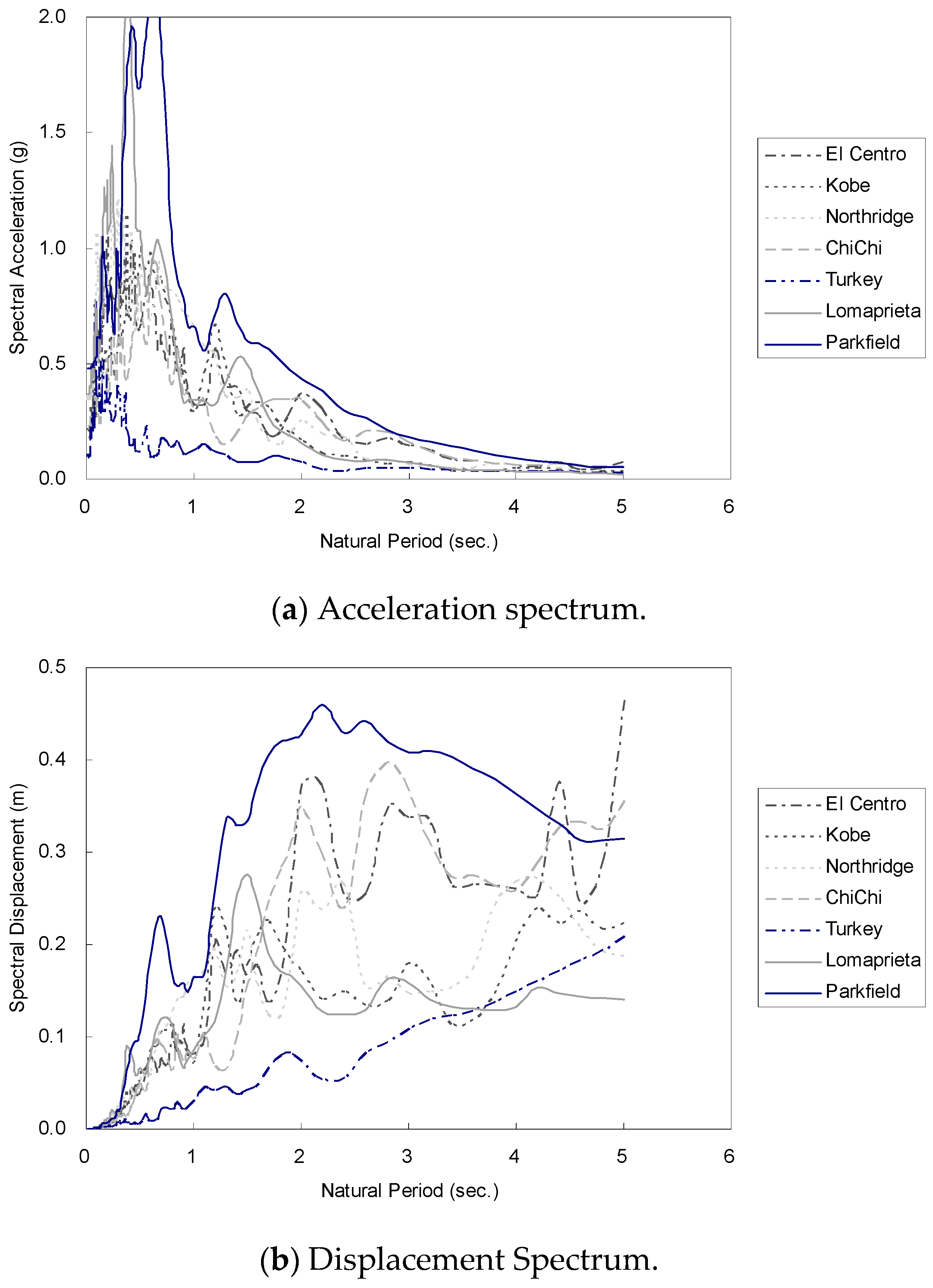
The detailed characteristics of the seven excitation data including the peak ground acceleration (PGA), the peak ground velocity (PGV), the peak ground displacement (PGD), differential time (DT) and total seismic excitation duration are summarized in

Table 3. Input ground excitation data for the time-history analysis.

Ground Acceleration Recordings [30]
Earthquake	PGA (g)	PGV (m/s)	PGD (m)	DT (s)	Duration (s)
El Centro (May 19 1940)	0.215	0.302	0.239	0.010	40.00
Kobe (Jan. 16 1995)	0.212	0.279	0.076	0.010	40.96
Northridge (Jan. 17 1994)	0.344	0.406	0.150	0.020	40.00
Chi-Chi, Taiwan (Sep. 20 1999)	0.364	0.554	0.256	0.004	150.00
Kocaeli, Turkey (Aug. 17 1999)	0.376	0.795	0.705	0.010	60.00
Loma Prieta (Oct. 18 1989)	0.367	0.329	0.072	0.005	39.95
Parkfield (Jun. 28 1966)	0.476	0.751	0.225	0.010	43.69

. As can be seen from the table, they have different peak ground acceleration and displacement values. For example, the Parkfield excitation has the highest peak ground acceleration value, 0.476 g, and the Turkey excitation showed the largest peak ground displacement of 0.705 m. Figure 14 shows the acceleration and displacement spectra plotted using the seven excitation data.

4.3. Analysis Results and Interpretation

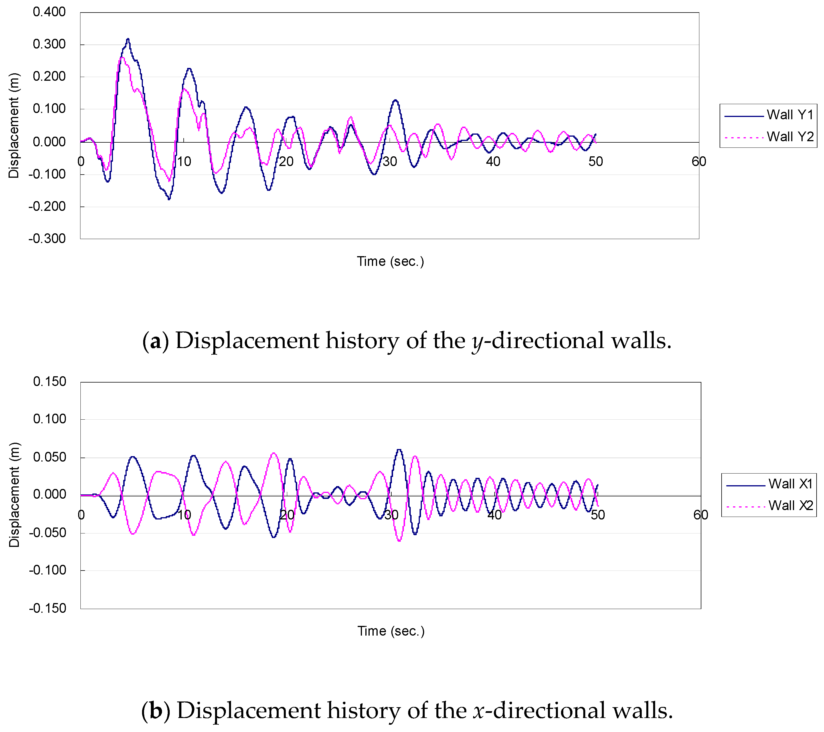
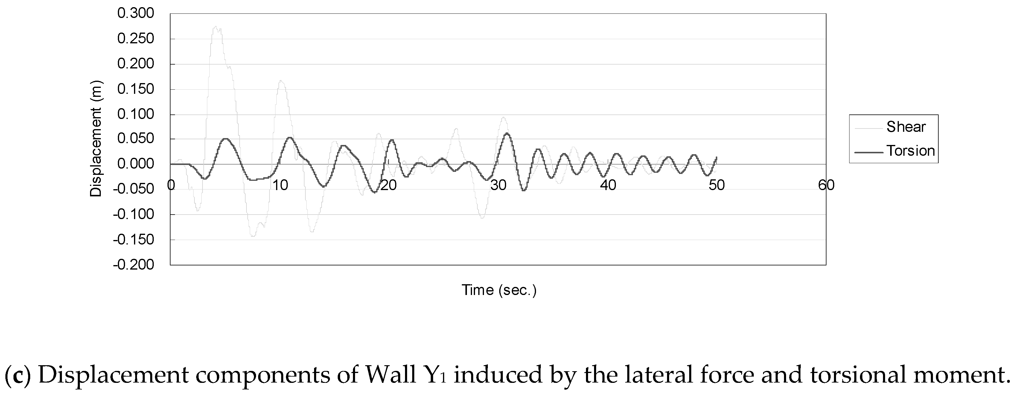
In this section, the effectiveness of the inelastic torsional deformation assessment procedure proposed in Section 3 is verified by comparing its results with those of the time history analyses of the model problem. Figure 15 shows the lateral displacement history for α = 1.3, β = 1.0 under El Centro excitation. The lateral displacements of the two y-directional walls are plotted in Figure 15a. In the figure, the solid line represents the displacement of the flexible side wall Y₁, and that of the stiff side wall Y₂ (dotted line). The difference between the lateral displacements of the two walls can be interpreted as the rotation of the asymmetric system. Figure 15b shows the lateral displacement history of the two x-directional walls, in which the lateral displacements of the two walls are of almost the same magnitude, but in the opposite direction. This indicates that the displacement history of the x-directional walls is mainly determined by the rotational behavior of the asymmetric system. In Figure 15c, the displacement of the flexible side wall Y₁ is decomposed into the component induced by lateral shear force and that by torsion, which are differentiated by a dark line and a light one, respectively. The sum of the two displacement components is equivalent to the solid line in Figure 15a.

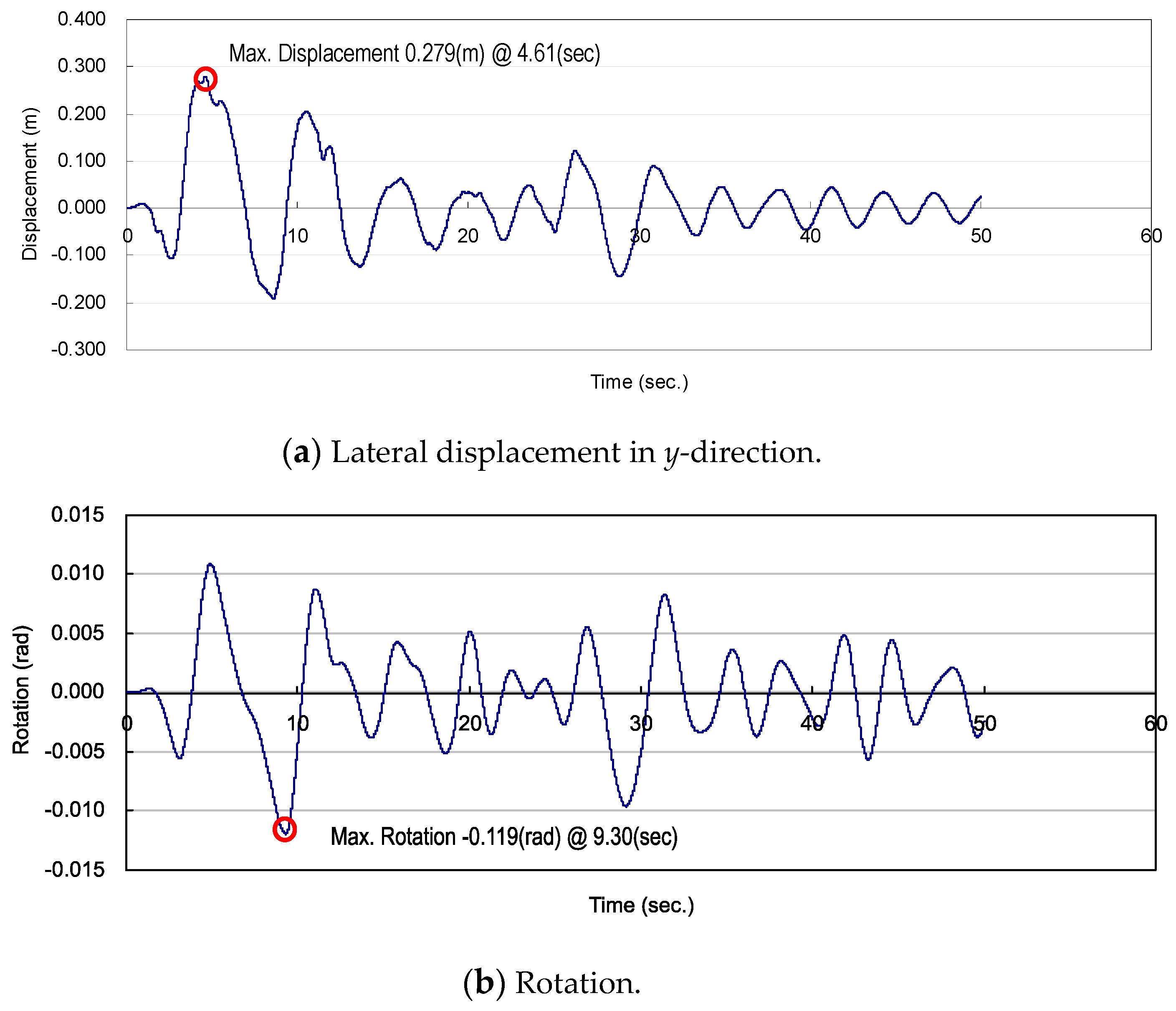
The results of Figure 15 are replotted in Figure 16, which presents the lateral displacement and rotation history estimated at the mass center of the asymmetric model problem. The maximum lateral displacement of 0.279 m occurs at 4.61 s, while the maximum rotation of −0.0119 rad occurs at 9.30 s. This clearly indicates that the two peak values do not occur simultaneously due to the dynamic effect on the structure by the excitation loading.

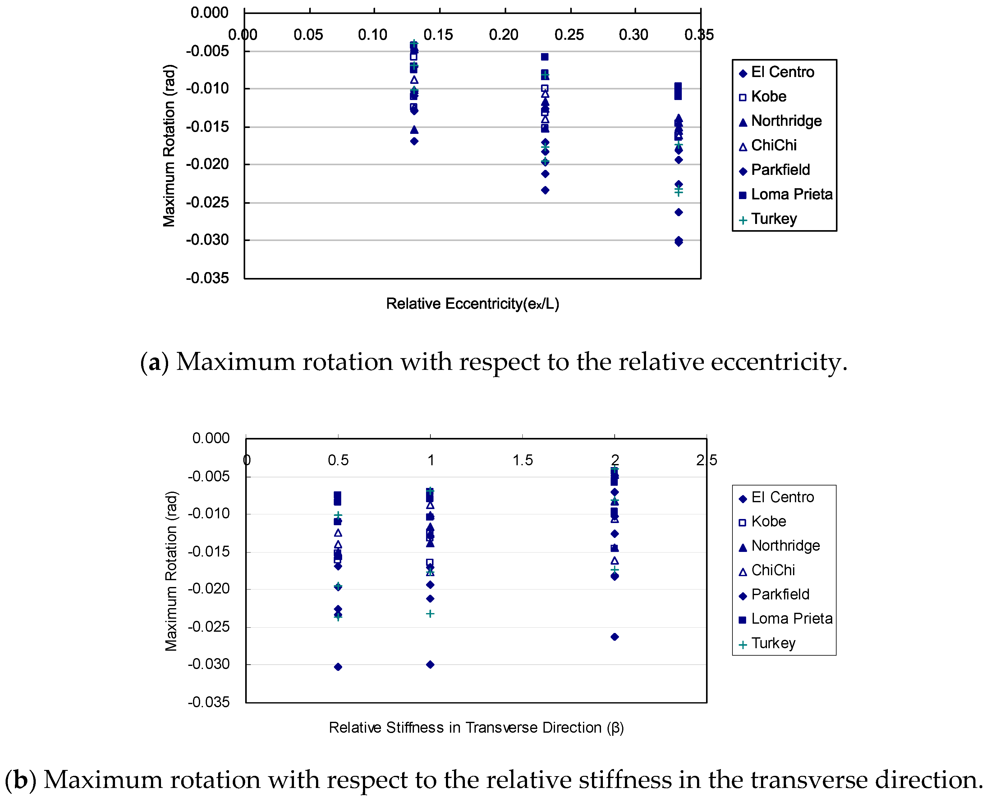
The maximum rotations of the 63 time history analysis simulations are plotted with respect to the relative eccentricity (e_x/L) and relative stiffness in the transverse direction (β) in Figure 17a,b, respectively. It can be noted from Figure 17a that the maximum rotations of all 63 simulations show an increasing trend with increasing relative eccentricity. As already discussed in Section 4.2, β can be regarded as the torsional constraint ratio, and thus Figure 17b clearly indicates that the maximum rotations of the time history analyses decrease as β is increased.

Table 4. Results of the time history analysis, the proposed method and the linear elastic response. (El Centro).

α	β	Time History Analysis			Proposed Method			Linear Elastic Response
		Δcen_TH (m)	ϕcen_TH (rad)	Δflex_TH (m)	ϕcen_pro (rad)	Δflex_pro (m)	Relative Error (%)	ϕcen_elas (rad)	Δflex_elas (m)	Relative Error (%)
1.30	0.50	0.275	−0.019	0.369	−0.010	0.324	−12.13	−0.007	0.308	−16.57
	1.00	0.277	−0.012	0.338	−0.006	0.307	−9.17	−0.006	0.307	−9.14
	2.00	0.278	−0.010	0.326	−0.003	0.295	−9.56	−0.005	0.304	−6.88
1.60	0.50	0.269	−0.023	0.385	−0.019	0.363	−5.72	−0.012	0.329	−14.67
	1.00	0.271	−0.020	0.371	−0.012	0.329	−11.24	−0.011	0.326	−12.16
	2.00	0.276	−0.017	0.359	−0.007	0.309	−13.85	−0.010	0.324	−9.79
2.00	0.50	0.243	−0.028	0.386	−0.029	0.388	0.45	−0.017	0.326	−15.46
	1.00	0.249	−0.027	0.383	−0.018	0.341	−10.87	−0.016	0.328	−14.46
	2.00	0.262	−0.024	0.382	−0.011	0.316	−17.26	−0.014	0.333	−12.71
Average of absolute relative errors					-		10.03	-		12.43

provides the results of the time history analysis, the proposed method and the linear elastic torsional response computed for the 9 different combinations of α and β discussed in Section 4.2. The ground motion applied in the time history analysis is the El Centro excitation. In the time history analysis results of the table, the maximum displacement in the y-direction at the center of mass (Δ_{cen_TH}) was given, and then the rotation at the center of mass (ϕ_{cen_TH}) and the displacement on the flexible side wall Y₁ (Δ_{flex_TH}) corresponding to this displacement were listed. The maximum displacement Δ_{cen_TH} was taken as the target displacement in the results of the proposed method and the linear elastic response, and it was used to compute the rotation at the center of mass (ϕ_{cen_pro} and ϕ_{cen_elas}) and the displacement on the flexible side wall Y₁ (Δ_{flex_pro} and Δ_{flex_elas}) by each of the two methods, respectively. In addition, the relative error of the displacement on the wall Y₁ was calculated by taking the corresponding time history analysis value Δ_{flex_TH} as the reference value. The average of the absolute relative errors for the other two methods are also provided at the end of the table.

The results of Table 4 show that the proposed method slightly underestimated the displacement on the flexible side wall in general, and its average of the absolute relative errors (relative error average) is smaller than that of the linear elastic response. The reason why both the proposed and linear elastic methods underestimate the flexible side wall displacement seems to be that they are all based on simple static analysis procedure and have some limitations in accurately capturing the effect of complex dynamic behavior. Therefore, some safety margin needs to be introduced, if the proposed approach is applied to the design of an actual plan-asymmetric structure. The ratio between the two average values is 80.7% (=10.03/12.43 × 100%). A similar trend can be found from

Table 5. Results of the time history analysis, the proposed method and the linear elastic response. (Kobe).

α	β	Time History Analysis			Proposed Method			Linear Elastic Response
		Δcen_TH (m)	ϕcen_TH (rad)	Δflex_TH (m)	ϕcen_pro (rad)	Δflex_pro (m)	Relative Error (%)	ϕcen_elas (rad)	Δflex_elas (m)	Relative Error (%)
1.30	0.50	0.127	−0.012	0.188	−0.008	0.169	−9.94	−0.003	0.142	−24.38
	1.00	0.125	−0.011	0.181	−0.005	0.151	−16.74	−0.003	0.139	−23.43
	2.00	0.130	−0.007	0.167	−0.003	0.144	−13.48	−0.002	0.142	−14.99
1.60	0.50	0.110	−0.017	0.195	−0.013	0.175	−10.39	−0.005	0.134	−31.11
	1.00	0.111	−0.016	0.194	−0.010	0.160	−17.31	−0.004	0.133	−31.19
	2.00	0.121	−0.011	0.174	−0.006	0.149	−14.12	−0.004	0.142	−18.41
2.00	0.50	0.087	−0.018	0.176	−0.011	0.142	−19.57	−0.006	0.117	−33.62
	1.00	0.098	−0.017	0.182	−0.011	0.155	−14.58	−0.006	0.129	−29.15
	2.00	0.114	−0.012	0.172	−0.009	0.160	−6.75	−0.006	0.145	−15.64
Average of absolute relative errors					-		13.65	-		24.66

;

Table 6. Results of the time history analysis, the proposed method and the linear elastic response. (Northridge).

α	β	Time History Analysis			Proposed Method			Linear Elastic Analysis
		Δcen_TH (m)	ϕcen_TH (rad)	Δflex_TH (m)	ϕcen_pro (rad)	Δflex_pro (m)	Relative Error (%)	ϕcen_elas (rad)	Δflex_elas (m)	Relative Error (%)
1.30	0.50	0.161	−0.012	0.221	−0.009	0.205	−7.28	−0.004	0.180	−18.45
	1.00	0.162	−0.008	0.204	−0.005	0.189	−7.48	−0.004	0.180	−11.96
	2.00	0.162	−0.009	0.209	−0.003	0.177	−15.31	−0.003	0.177	−15.36
1.60	0.50	0.157	−0.011	0.211	−0.017	0.241	14.13	−0.007	0.192	−9.13
	1.00	0.157	−0.012	0.216	−0.010	0.209	−3.25	−0.006	0.189	−12.59
	2.00	0.158	−0.012	0.217	−0.006	0.188	−13.56	−0.005	0.185	−14.57
2.00	0.50	0.150	−0.016	0.228	−0.021	0.257	12.93	−0.010	0.201	−11.65
	1.00	0.150	−0.016	0.232	−0.017	0.233	0.59	−0.009	0.197	−14.93
	2.00	0.151	−0.018	0.243	−0.010	0.199	−17.98	−0.008	0.192	−20.91
Average of absolute relative errors					-		10.28	-		14.39

, which provide the results obtained by applying Kobe and Northridge excitations, respectively. In this case, the relative error averages of the proposed method are even much smaller than those of the linear elastic response. In the case of the Kobe excitation, the relative error average of the proposed method is only 55.4% of the linear elastic response value (=13.65/24.66 × 100%). Similarly, the former is only 71.4% of the latter (=10.28/14.39 × 100%) in the case of the Northridge excitation.

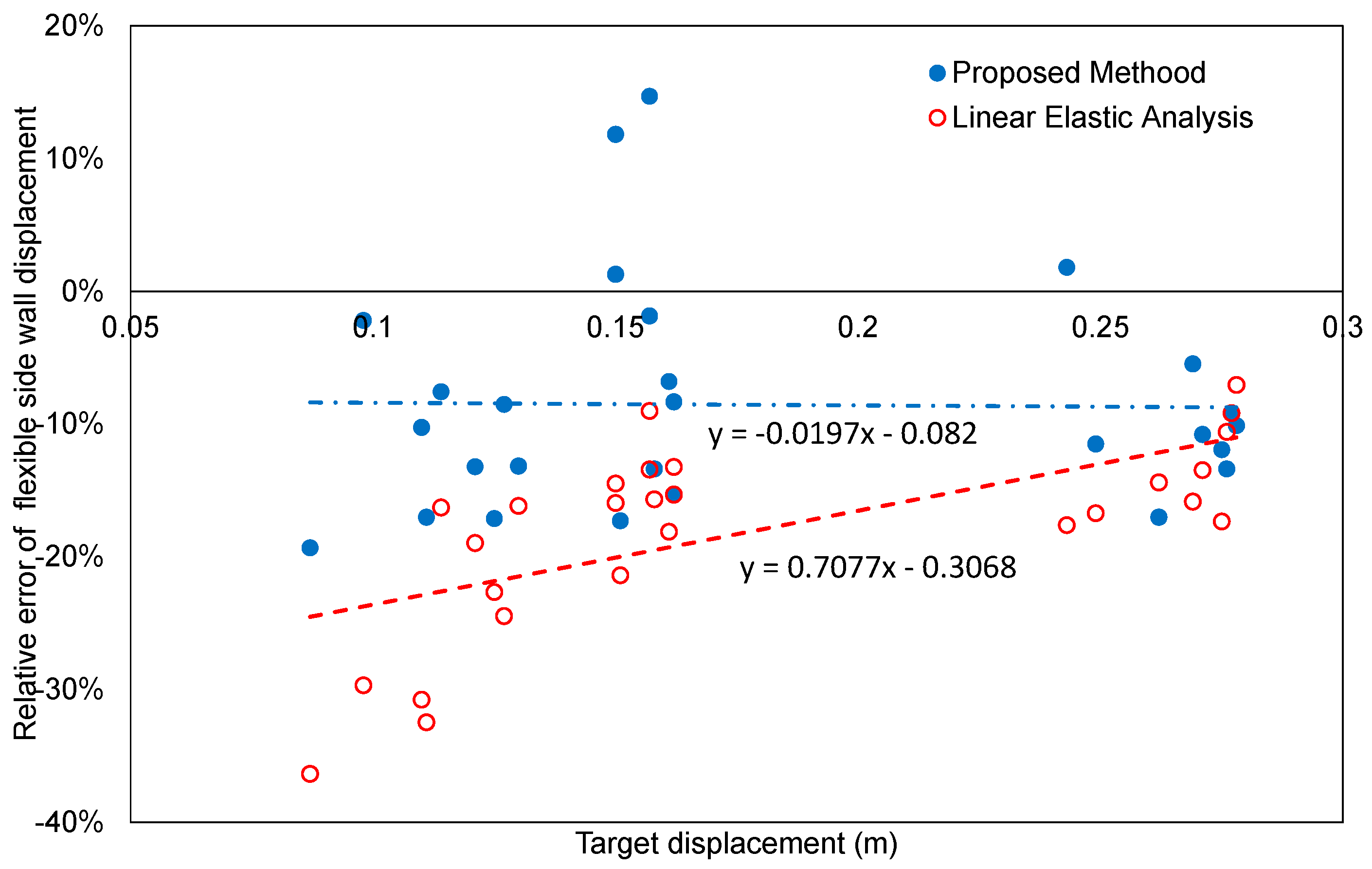
Figure 18 plots the relative errors of the flexible side wall displacement of all 27 data points listed in Table 4, Table 5 and Table 6 with respect to the target displacement (Δ_{cen_TH}) for the proposed method and the linear elastic response. A linear regression analysis is performed on each set of the results computed with the two methods by having the target displacement as an independent variable, and their regression lines are drawn in the figure. The coefficients of determination obtained by the regression results by the proposed and linear elastic methods are 0.0002 and 0.4198, respectively. It can be seen from the results of the figure that the linear regression line of the proposed method is located closer to the horizontal axis than that of the linear elastic response in all ranges of the target displacement, confirming that the proposed method can provide more accurate solutions than the linear elastic response.

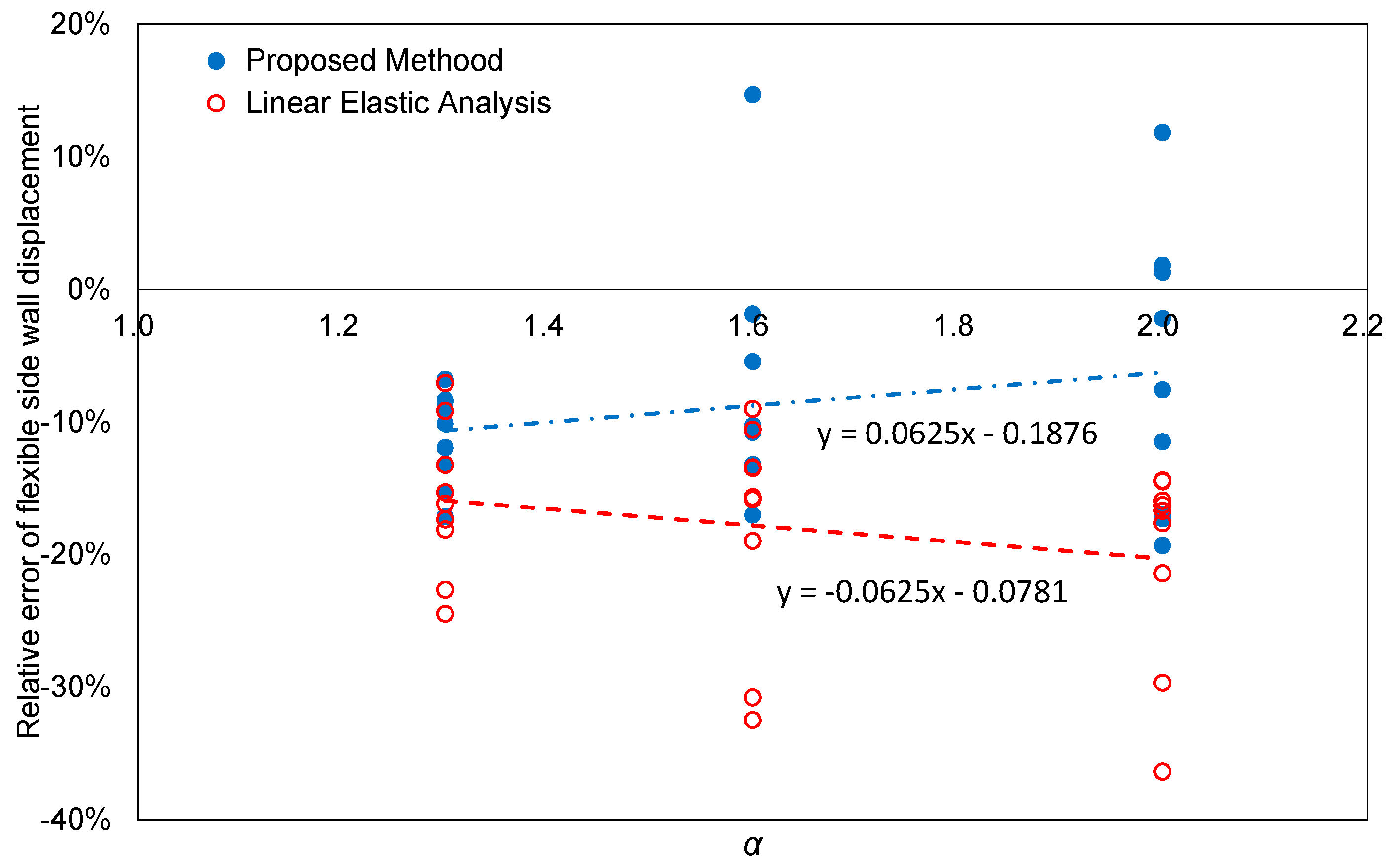
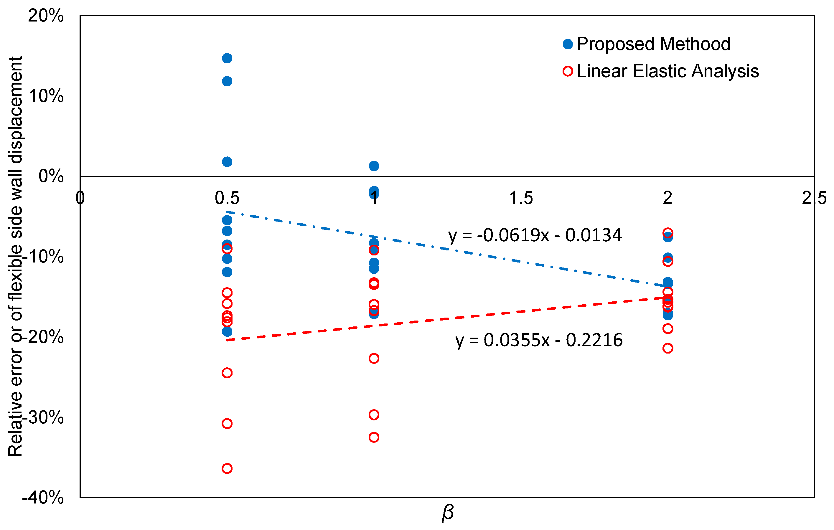
In Figure 19, the two sets of the results presented in Figure 18 are plotted with respect to the ratio of the stiff wall stiffness to that of the flexible wall (α), and the linear regression analysis is performed again. The coefficients of determination obtained by the regression results by the proposed and linear elastic methods are 0.0473 and 0.063, respectively. It can be seen from the figure that the linear regression line of the proposed method gets closer to the horizontal axis with increasing α. This means that the proposed method is able to provide more accurate solutions when the level of plan-asymmetry gets higher. Similarly, Figure 20 plots the same data as in Figure 18; Figure 19 with respect to β. The coefficients of determination obtained by the regression results by the proposed and linear elastic methods are 0.2191 and 0.0961, respectively. Since the regression line of the proposed method gets closer to the horizontal axis with decreasing β, the proposed method can provide more accurate solutions as the level of torsional constraint gets smaller, and thus the same conclusion can be made as in Figure 19.

5. Conclusions

In this paper, we proposed a simple method that can accurately assess the inelastic lateral displacement and rotation of plan-asymmetric wall structures. The relationship between the lateral displacement and rotation was obtained by considering the inelastic behavior of asymmetric structures. This relationship was presented and interpreted in the displacement-rotation (D-R) coordinate system. This coordinate system was first introduced in this paper and very conveniently describes the inelastic torsional behavior of the asymmetric structure. The validity of the proposed method was verified by comparing its predictions and inelastic time-history analysis results for a model problem. The main conclusions of this paper are as follows:

• Most of the current seismic design codes such as IBC, NZS, NBCC and Eurocode are based on the force-based design approach and introduce the concept of the design eccentricity consisting of static and accidental eccentricities. They do not properly consider the inelastic deformation and actual failure mechanism of plan-asymmetric structures. As a result, they may require excessive strength and stiffness for lateral force resisting components.
• The inelastic torsional response assessment procedure proposed in this paper shows that the linear elastic approach may both underestimate the torsional rotation at the initial yielding stage and overestimate it at the post yielding stage, resulting in inaccurate estimation of the torsional response over the entire inelastic range.
• The stiffness of the transverse wall may affect the overall yielding procedure of asymmetric structures. As a result, first yielding may occur even in the stiff side wall if the transverse wall stiffness and yield displacement are determined mainly by its length. This effect is not considered by any of the current code provisions such as IBC and Eurocode, while the procedure proposed in this study can handle it properly.
• A comparison between the results of the time history analysis and the predictions of the proposed method for the model problem under three different seismic excitations (El Centro, Kobe and Northridge) shows that the relative error averages of the proposed method range approximately from 10.0% to 13.7% and are considerably smaller than those of the linear elastic response. It also indicates that the proposed method is able to provide more accurate solutions if the level of plan-asymmetry is higher.
• In general, the proposed method underestimates the flexible side wall displacement as it is based on simple static analytical procedure and has some limitations in accurately capturing the effect of complex dynamic behavior. Therefore, some safety margin needs to be introduced, if it is applied to the design of an actual plan-asymmetric structure.

Currently, we are extending the inelastic torsional response assessment approach proposed in this paper and developing an iterative method utilizing the secant stiffness of each wall for the effective estimation of the inelastic torsional behavior of complex plan-asymmetric structures. This approach also can be incorporated into the adaptive push-over analysis discussed in [31,32,33,34] that explicitly considers the nonlinear torsional and higher-mode effects for the analysis of multi-story structures.

References

- Mitchell, D.; Adams, J.; Devall, R.H.; Lo, R.C.; Weichert, D. Lessons from the 1985 Mexican Earthquake. Can. J. Civ. Eng. 1986, 13, 535–557. [Google Scholar] [CrossRef]
- Wood, S.L.; Stark, R.; Greer, S.A. Collapse of Eight-Story RC Building during 1985 Chile Earthquake. ASCE J. Struct. Eng. 1991, 117, 600–619. [Google Scholar] [CrossRef]
- Mitchell, D.; Tinawi, R.; Redwood, R.G. Damage to Buildings Due to the 1989 Loma-Prieta Earthquake—A Canadian Code Perspective. Can. J. Civ. Eng. 1990, 17, 813–834. [Google Scholar] [CrossRef]
- Mitchell, D.; DeVall, R.H.; Kobayashi, K.; Tinawi, R.; Tso, W.K. Damage to concrete structures due to the January 17, 1995, Hyogo-ken Nanbu (Kobe) earthquake. Can. J. Civ. Eng. 1996, 23, 757–770. [Google Scholar] [CrossRef]
- International Code Council. 2015 International Building Code; International Code Council: Country Club Hills, IL, USA, 2014. [Google Scholar]
- Standards New Zealand. Structural Design Actions. Part 5, Earthquake Actions: New Zealand; NZS 1170; Standards New Zealand: Wellington, New Zealand, 2004. [Google Scholar]
- National Research Council Canada and Canadian Commission on Building and Fire Codes. National Building Code of Canada, 2015; Canadian Commission on Building and Fire Codes, National Research Council of Canada: Ottawa, ON, Canada, 2015. [Google Scholar]
- British Standards Institution and European Committee for Standardization. Eurocode 8, Design of Structures for Earthquake Resistance Part 1, General Rules, Seismic Actions and Rules for Buildings; British Standards Institution: London, UK, 2004. [Google Scholar]
- Goel, R.K.; Chopra, A.K. Dual-Level Approach for Seismic Design of Asymmetric-Plan Buildings. ASCE J. Struct. Eng. 1994, 120, 161–179. [Google Scholar] [CrossRef]
- Duan, X.N.; Chandler, A.M. An optimized procedure for seismic design of torsionally unbalanced structures. Earthq. Eng. Struct. Dyn. 1997, 26, 737–757. [Google Scholar] [CrossRef]
- Humar, J.L.; Kumar, P. Effect of orthogonal inplane structural elements on inelastic torsional response. Earthq. Eng. Struct. Dyn. 1999, 28, 1071–1097. [Google Scholar] [CrossRef]
- Paulay, T. Displacement-based design approach to earthquake-induced torsion in ductile buildings. Eng. Struct. 1997, 19, 699–707. [Google Scholar] [CrossRef]
- Paulay, T. Torsional mechanisms in ductile building systems. Earthq. Eng. Struct. Dyn. 1998, 27, 1101–1121. [Google Scholar] [CrossRef]
- De Stefano, M.; Faella, G.; Ramasco, R. Inelastic seismic response of one-way plan-asymmetric systems under bi-directional ground motions. Earthq. Eng. Struct. Dyn. 1998, 27, 363–376. [Google Scholar] [CrossRef]
- De la Llera, J.C.; Chopra, A.K. Inelastic behavior of asymmetric multistory buildings. ASCE J. Struct. Eng. 1996, 122, 597–606. [Google Scholar] [CrossRef]
- Lin, J.L.; Tsai, K.C. Simplified seismic analysis of asymmetric building systems. Earthq. Eng. Struct. Dyn. 2007, 36, 459–479. [Google Scholar] [CrossRef]
- Panagiotou, M.; Restrepo, J.I.; Schoettler, M.; Kim, G. Nonlinear cyclic truss model for reinforced concrete walls. ACI Struct. J. 2012, 109, 205–214. [Google Scholar]
- Lu, Y.; Panagiotou, M. Three-dimensional cyclic beam-truss model for nonplanar reinforced concrete walls. ASCE J. Struct. Eng. 2014, 140, 04013071. [Google Scholar] [CrossRef]
- Cho, B.H.; Hong, S.G.; Ha, T.H.; Kim, D.J. Seismic evaluation of asymmetric wall systems using a modified three-dimensional capacity spectrum method. J. Vibroengineering 2015, 17, 4366–4376. [Google Scholar]
- Bento, R.; Bhatt, C.; Pinho, R. Using nonlinear static procedures for seismic assessment of the 3D irregular SPEAR building. Earthq. Struct. 2010, 1, 177–195. [Google Scholar] [CrossRef]
- Kreslin, M.; Fajfar, P. Seismic evaluation of an existing complex RC building. Bull. Earthq. Eng. 2010, 8, 363–385. [Google Scholar] [CrossRef]
- Ferraioli, M. Case study of seismic performance assessment of irregular RC buildings: Hospital structure of Avezzano (L’Aquila, Italy). Earthq. Eng. Eng. Vib. 2015, 14, 141–156. [Google Scholar] [CrossRef]
- Anagnostopoulos, S.A.; Kyrkos, M.T.; Stathopoulos, K.G. Earthquake induced torsion in buildings: Critical review and state of the art. Earthq. Struct. 2015, 8, 305–377. [Google Scholar] [CrossRef]
- Wallace, J.W. A Methodology for Seismic Design of RC Shear Walls. ASCE J. Struct. Eng. 1994, 120, 863–884. [Google Scholar] [CrossRef]
- Paulay, T. An estimation of displacement limits for ductile systems. Earthq. Eng. Struct. Dyn. 2002, 31, 583–599. [Google Scholar] [CrossRef]
- MATLAB 2014a; The MathWorks, Inc.: Natick, MA, USA, 2014.
- Mazzoni, S.; McKenna, F.; Scott, M.H.; Fenves, G.L. Open System for Earthquake Engineering Simulation: User Command, Language Manual; PEER Center, UC: Berkeley, CA, USA, 2009. [Google Scholar]
- Priestley, M.J.N.; Grant, D.N. Viscous damping in seismic design and analysis. J. Earthq. Eng. 2005, 9, 229–255. [Google Scholar] [CrossRef]
- Kunnath, S.K.; Reinhorn, A.M.; Park, Y.J. Analytical modeling of inelastic seismic response of R/C structures. ASCE J. Struct. Eng. 1990, 116, 996–1017. [Google Scholar] [CrossRef]
- Pacific Earthquake Engineering Research Center. PEER Ground Motion Database. Available online: https://ngawest2.berkeley.edu/ (accessed on 7 January 2017).
- Kaatsız, K.; Sucuolu, H. Generalized force vectors for multi-mode pushover analysis of torsionally coupled systems. Earthq. Eng. Struct. Dyn. 2014, 43, 2015–2033. [Google Scholar] [CrossRef]
- Ferraioli, M. Multi-mode pushover procedure for deformation demand estimates of steel moment-resisting frames. Int. J. Steel Struct. 2017, 17, 653–676. [Google Scholar] [CrossRef]
- Ferraioli, M.; Lavino, A.; Mandara, A. An adaptive capacity spectrum method for estimating seismic response of steel moment-resisting frames. Ing. Sismica Int. J. Earthq. Eng. 2016, 1–2, 47–60. [Google Scholar]
- Colajanni, P.; Cacciola, P.; Potenzone, B.; Spinella, N.; Testa, G. Nonlinear and linearized combination coefficients for modal pushover analysis. Ing. Sismica Int. J. Earthq. Eng. 2017, 3–4, 93–112. [Google Scholar]
Figure 1.
Representative asymmetric wall structures under the application of a lateral force and its deformed shape.
Figure 2.
Lateral displacement-rotation (D-R) coordinate system.
Figure 3.
Model problem of a plan-asymmetric structure.
Figure 4.
Force-displacement relationship between the lateral force resisting wall components.
Figure 5.
Yielding procedure: Linear elastic stage.
Figure 6.
Yielding procedure: First inelastic stage.
Figure 7.
Yielding procedure: Second inelastic stage.
Figure 8.
Comparison between inelastic torsional responses using the current design code and proposed approach.
Figure 9.
Example problem for the investigation of a transverse wall stiffness effect.
Figure 10.
Effect of transverse wall stiffness on the overall yielding procedure of asymmetric structures.
Figure 11.
Modeling of an individual structural wall for the time history analysis.
Figure 12.
Diagonal truss modeling using two parallel elements.
Figure 13.
Response of the model problem subjected to cyclic static loading.
Figure 14.
Spectral acceleration and displacement of the excitation data.
Figure 15.
Lateral displacement history of each wall component (El Centro, α = 1.3, β = 1.0).
Figure 16.
Lateral displacement and rotation history estimated at the center of mass (El Centro, α = 1.3, β = 1.0).
Figure 17.
Effects of the relative eccentricity and relative stiffness in the transverse direction on the maximum rotations obtained by the time history analysis simulations.
Figure 18.
Comparison between the relative errors of the flexible side wall maximum displacement computed by the two methods with respect to the target displacement.
Figure 19.
Comparison between the relative errors of the flexible side wall maximum displacement computed by the two methods with respect to α.
Figure 20.
Comparison between the relative errors of the flexible side wall maximum displacement computed by the two methods with respect to β.