Multi-Objective Defocus Robust Source and Mask Optimization Using Sensitive Penalty


Key Laboratory of Photoelectronic Imaging Technology and System of Ministry of Education of China, School of Optics and Photonics, Beijing Institute of Technology, Beijing 100081, China
*
Author to whom correspondence should be addressed.
Appl. Sci. 2019, 9(10), 2151; https://doi.org/10.3390/app9102151
Submission received: 12 April 2019
/
Revised: 12 May 2019
/
Accepted: 17 May 2019
/
Published: 27 May 2019
(This article belongs to the Section Optics and Lasers)
Abstract
:The continuous decrease in the size of lithographic technology nodes has led to the development of source and mask optimization (SMO) and also to the control of defocus becoming stringent in the actual lithography process. Due to multi-factor impact, defocusing is always changeable and uncertain in the real exposure process. But conventional SMO assumes the lithography system is ideal, which only compensates the optical proximity effect (OPE) in the best focus plane. Therefore, to solve the inverse lithography problem with more uniformity of pattern in different defocus variations, we proposed a defocus robust SMO (DRSMO) approach that is driven by a defocus sensitivity penalty function for the first time. This multi-objective optimization samples a wide range of defocus disturbances and it can be proceeded by the mini-batch gradient descent (MBGD) algorithm effectively. The simulation results showed that a more robust defocus source and mask can be designed through DRSMO optimization. The defocus sensitivity factor sβ maximally decreased 63.5% compared to conventional SMO, and due to the low error sensitivity and the depth of defocus (DOF), the process window (PW) was further enlarged effectively. Compared to conventional SMO, the exposure latitude (EL) maximally increased from 4.5% to 10.5% and DOF maximally increased 54.5% (EL = 5%), which proved the validity of the DRSMO method in improving the focusing performance.
1. Introduction
With the shrink in critical dimension (CD), the impact of the optical proximity effect (OPE) become obvious, it causes distortion in the exposure pattern and reduction of pattern fidelity and contrast, so that it must be corrected effectively. Besides, continuous shrinking also allows for control of the defocus in lithography to become increasingly stringent. In actual lithography processes, defocus is always uncertain at the wafer level, because of the unevenness of the wafer surface [1]. In addition, aberrations, thermal aberrations [2], thermal mask effects [3], and thick mask effects [4] all inevitably cause best-focus plane constant shift and further increase the OPE in off-focus conditions. Meanwhile, the continuous shrinkage of technology nodes has promoted the introduction of resolution enhancement technology (RET). Conventional RET, such as optical proximity correction (OPC) and source and mask optimization (SMO), generate the best exposure conditions by optimizing mask or simultaneously optimizing source and mask, respectively [5,6]. However, general RET methods assume the lithography system is ideal, which only compensates the OPE in the nominal condition [7,8,9]. But, with CD shrinkage, it results in the imaging quality becoming more sensitive to defocus, thus requiring RET methods corresponding to off-focus conditions. Therefore, to tackle the focus variation, an analytical defocus expansion function was derived to predict the defocus aerial image in an inverse lithography technology (ILT) framework [10], so that a variational lithography model (VLIM) is derived to take into account exposure dose and focus variations [11]. Meanwhile, we previously proposed the source–mask-numerical aperture (NA) co-optimization (SMNO) method to extend the depth of defocus (DOF) by fine-tuning the NA [12,13], but it inevitably sacrificed resolution due to the reduction of NA. In addition, Peng et al. [14] also studied SMO methods to improve the pattern fidelity in the case of an assigned defocus plane which operated at 100 nm defocusing, and our subsequent works have drawn on this approach [15,16], but it is hard to ensure global fidelity in different defocus variations. Thus, Jia et al. [17,18,19,20,21] proposed statistical variations-based OPC and SMO methods to improve global fidelity at different defocus variations.
Unfortunately, the above methods found it hard to improve the uniformity of exposure patterns within the DOF, so that the optimized system still had relatively high sensitivity to defocusing. To eliminate changeable and uncertain defocusing due to the presence of multiple factors effectively, it requires the reduction of defocusing sensitivity for optimized systems. Therefore, to the best of our ability to minimize the defocusing sensitivity, we propose a defocus robust SMO (DRSMO) approach that is driven by a new multi-objective optimization strategy. In our method, the total cost function is composed of expectation fidelity and expectation sensitivity in different defocus disturbances. In addition, the expectation sensitivity penalty function is introduced into an inverse optimization framework for the first time to constrain the uniformity of aerial images to defocus in different disturbances, so that more robust source and mask are designed through this optimization. Compared to conventional SMO approaches, the simulation results confirmed that DRSMO can further reduce defocus sensitivity and improve process robustness. The defocus sensitivity factor maximally decreased 63.5% compared to conventional SMO, and the DOF corresponding to EL = 5% maximally increased 54.5%, EL maximally increased from 4.5% to 10.5% as well. It means that larger exposure tolerances were in the actual lithography process via DRSMO. In addition, this paper also discusses the established optimization problem which was solved by the stochastic gradient descent (SGD) algorithm and mini-batch gradient descent (MBGD) algorithm. Optimization results show that due to the wide sampling range of defocus disturbances, it is easy to fall into the local optimal solution by SGD but converge well when introduced to MBGD.
The remainder of the paper is organized as follows. In Section 2, the introduction of the forward imaging model, the inverse optimization problem driven by the new multi-objective cost function, and the multi-objective optimization process by different algorithms are described. In Section 3, the simulation conditions and simulation results are presented.
2. DRSMO Modeling
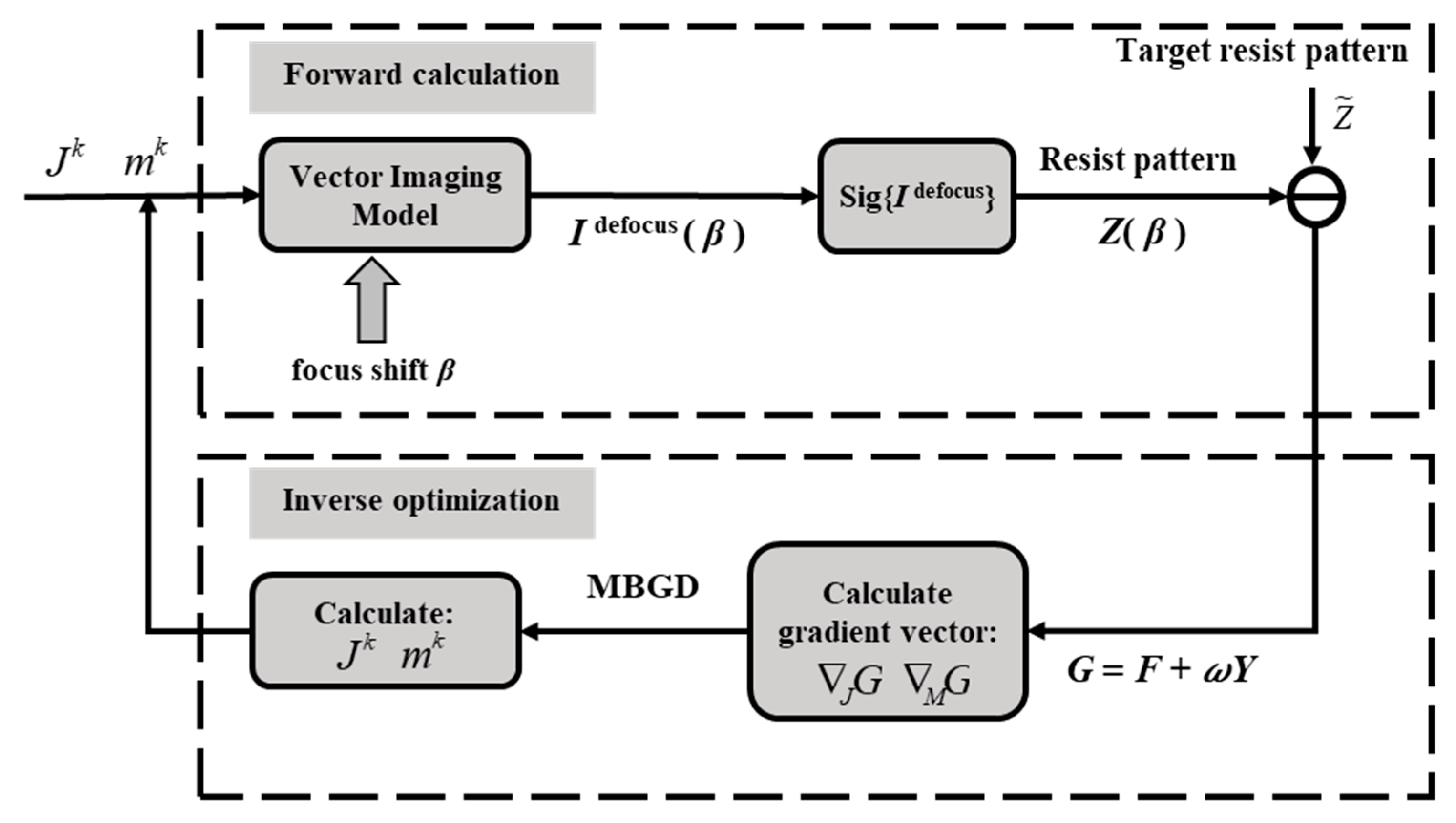
Figure 1 illustrates the DRSMO optimization framework which is composed of the forward calculation to evaluate pattern fidelity and the inverse optimization to update the source and mask parameters. In current lithography processes, source and mask are freeform pixel-based configurations. Therefore, both the source and mask can be represented by matrix form and , respectively. Each source element represent normalized light intensity and each mask element is subject to 0–1 binary distribution. To overcome the complexity of the constrained optimization problem, a parameters transfer was made to convert and to unconstrained sources mask parameters and (see Appendix B and Equation (A9)) in the kth iteration, respectively [8].
As for the forward calculation process, the printed resist pattern was calculated by the given light source and mask parameters through the corresponding physical process. Then, the printed pattern was compared with the target resist pattern to evaluate the pattern fidelity and CD error. Under the Abbe imaging principle, the aerial image that takes into account defocusing can be represented as . For the model-based SMO method, the scalar imaging model is inaccurate in hyper-NA (NA > 1) immersion lithography systems [22]. Thus, we previously studied the vector imaging model for aerial image calculation [16], and it can be formulated as
where is the summation of all the source intensity and is used as a normalization factor. is the electric fields (x-, y-, and z-directions) in the exposure plane which can be expressed as
where nw is the index of refraction, the magnification of R = 4 normally,
is the vector matrix for hyper-NA systems, is the irradiance correction factor, is the ideal pupil filter, is the mask diffraction near field, is the electric field of the source that is represented by a 2 × 1 vector. Operators , , and are represented by matrix entry-by-entry multiplication, forward Fourier transform, and inverse Fourier transform, respectively.
It should be noted that the impact of defocusing on resulting aerial image Def can be described as an aberration of a sort [23]. This causes a distribution of the phase change on the ideal aperture which can be described as
where is the direction cosine in the propagation direction and is the defocus value.
Next, the resist image was adopted to the continuous derivable sig model [24], which can be expressed as
where indicates the steepness of the sigmoid function, and is the threshold.
2.1. DRSMO Inverse Optimization Framework
As for the inverse optimization process in Figure 1, it is a continuous update source and mask parameter to meet the final target resist pattern and overcome the OPE. The inverse optimization process of DRSMO relies on the corresponding cost function establishment. In DRSMO, the multi-objective cost function is composed of the statistics expected in plentiful defocus disturbances, and the total cost function can be divided into two parts: the pattern fidelity part and defocus sensitivity part.
The pattern fidelity part is in light of Jia’s [19] approach, which is defined as the expectation of the Euclidean distance between the target resistance pattern and the resistance pattern in plentiful defocusing disturbances. It can be formulated as
where is a stochastic variable representing defocusing disturbances. It is subject to a certain range of evenly distributed disturbances, namely, . represents the whole training set. It should be noted that the sample range of ±α is selected according to the actual situation, larger α can theoretically lead to wider DOFs, but too large a DOF will be beyond the potential of optimization and , , respectively. is the mathematical expectation.
To the core ideal of DRSMO is introduced the defocus sensitivity penalty function, which aims at minimizing the expected quadratic change ratio of the aerial image to defocusing and can be formulated as
This penalty function directly controls the change rate of the aerial image to the defocus, which improves the consistency of the pattern and CD in different defocus disturbances. Therefore, it is beneficial to optimize a more robust source and mask with a lower defocus sensitivity. Besides, due to the improvement of process robustness for the optimized system, the PW will also enlarge. Appendix A and Equation (A5) define the details about the analytical sensitivity penalty Yi, so that the total cost function consists of the weighted sum of F and Y.
where is the weighting factor of the sensitivity part. Typically, means the optimization only operates at the fidelity part . In Section 3, we will discuss that the optimization results only operate at the fidelity part or simultaneously operates at the fidelity part and sensitivity part.
2.2. DRSMO Optimization Algorithm
In our method, the DRSMO process can be regarded as a machine learning process, training variable as a stochastic disturbance in the cost function to solve this multi-objective optimization problem. Table 1 illustrates the optimization flow of the SGD and MBGD algorithm, respectively. In our previous works [25,26], SGD was adopted to calculate the gradient in a single training sample in each iteration with fast speed. However, due to the wider sample range of defocus disturbances, the SGD algorithm could not guarantee each iteration was conducted in the global optimal direction.
In order to give consideration to both optimization speed and accuracy, mini-batch gradient descent (MBGD) was proposed to traverse a part of the random defocus samples in each iteration, and is the batch number in each iteration [27]. Different from the SGD method, MBGD updates part of the training set, thus leading to a relatively correct search direction, so it is easier to converge to the global optimal solution.
Both the SGD and MBGD algorithm need to calculate the analytic gradient expression of cost function, which can be formulated as
where and are the gradient to the source parameter and mask pattern , respectively. We directed a large amount of study toward the derivation of the analytic gradient formula about sensitive penalty ∇JYi, ∇MYi, and more details can be found in Appendix B, Equations (A11) and (A13). Similarly, the expansion of , can be found in Appendix C, Equations (A19) and (A20).
3. Simulation Results and Discussion
3.1. Simulation Conditions
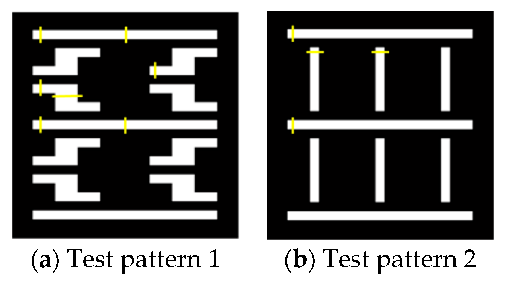
We illustrate the DRSMO method in two test patterns as shown in Figure 2. The critical dimension (CD) of each pattern was 45 nm. Resistance patterns and mask were represented by a 201 × 201 matrix with a resolution of 5.625 nm × 5.625 nm and 22.500 nm × 22.500 nm per pixel, respectively. The imaging system parameters were set to be λ = 193 nm and NA = 1.2. The freeform source was represented by a 21 × 21 matrix which uses TE-polarization illumination. In this paper, the whole training set consisted of 900 random sampling points in the range of (−100 nm, 100 nm), since this sample range was extremely larger than initial DOF, which was without optimization. Taking into account both optimization speed and accuracy, the batch number was set to be three per iteration and 300 iterations totally.
To evaluate the imaging fidelity, pattern error (PAE) refers to the Euclidean distance between the target pattern and the actual pattern in the resist. Generally, the smaller PAE means the higher fidelity of the lithographic imaging. It can be formulated as
where is the binary target resist pattern and is the actual resistance pattern under defocus . Meanwhile, to evaluate the defocusing sensitivity quantitatively, we defined the defocus sensitivity factor as the change ratio of PAE to defocusing
Moreover, to evaluate the process robustness in the actual exposure process, the PW was introduced to describe the restrictive relation between dose variation and focus variation. It was composed of two parameters, DOF and exposure latitude (EL). Exposure latitude is the allowable range of dose variation under a fixed defocus. Similarly, DOF is the largest acceptable defocus range under a fixed dose. Thus, PW consists of all pairs of DOF and EL which satisfy the exposure quality specification. Generally, taking the DOF when corresponding to ELs equal to 5% or 10% as process evaluation standard. Meanwhile, the PW representative calculation positions are marked at yellow lines in Figure 2.
3.2. Optimization Results and Analysis
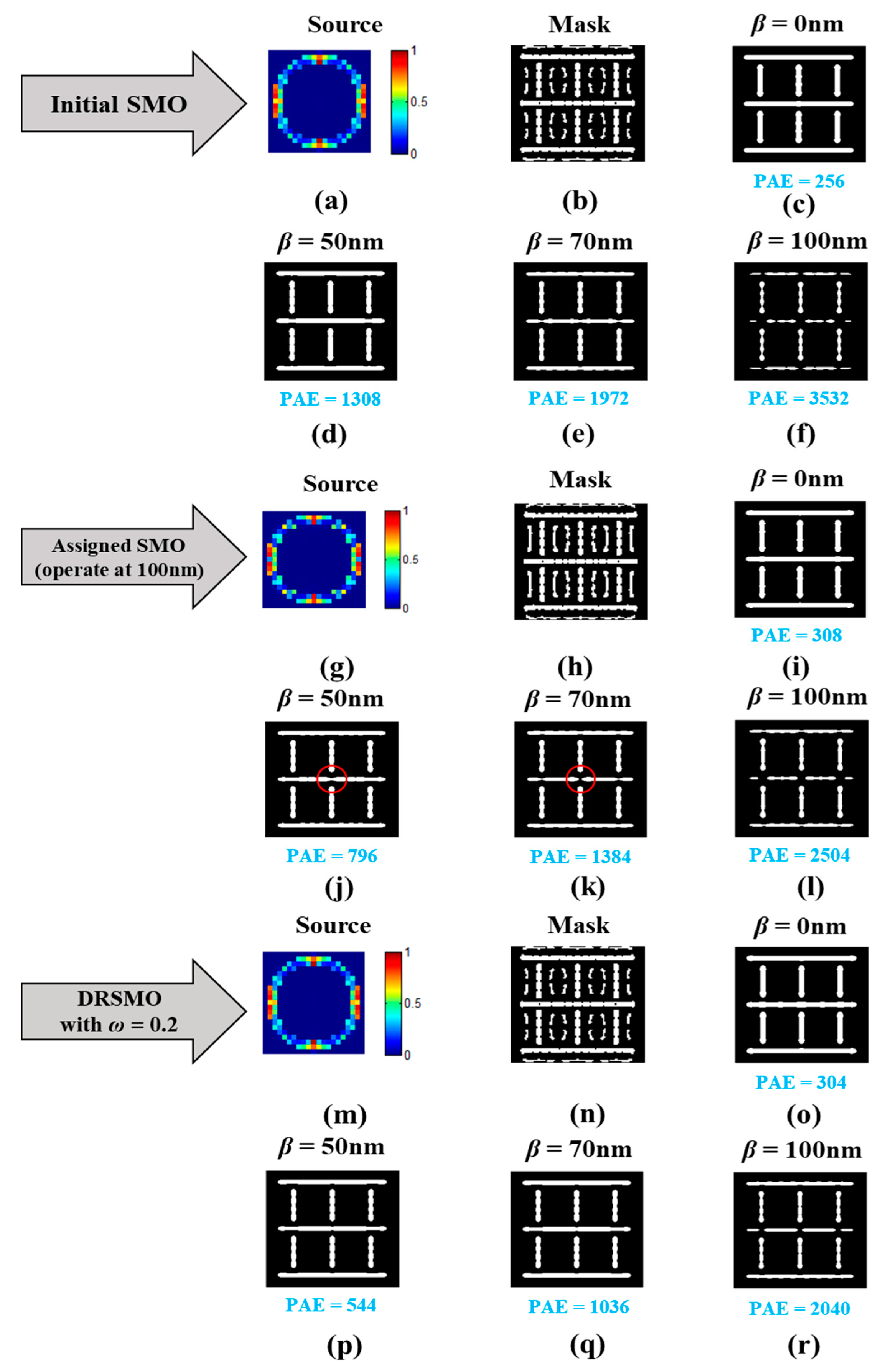
In order to illustrate the negative influence of defocus, Figure 3a–f shows the optimization proceeded by initial SMO which merely operated at the best focus plane [7], and the evaluation of the printed image was under different defocus planes. Figure 3a,b show the optimized source for initial SMO and optimized mask for initial SMO, respectively. Figure 3c shows the printed image at the best focus plane, and Figure 3d–f shows the printed image under 50 nm, 70 nm, and 100 nm defocus, respectively. It clearly shows that the PAE increased extremely with an increase of defocus, proving that the initial SMO could not compensate the defocus distortion because the cost function was not involved in the defocus term. However, the defocusing error inevitably existed in the actual lithography process, thereby it was necessary to gain a better and more robust defocusing via DRSMO.
Similarly, Figure 3g–l illustrates Peng’s [14] SMO method which merely operates at an assigned defocus plane (100 nm defocusing). In this method, the established cost function can be formulated as the weight sum of the nominal term and defocus term
Figure 3g,h show the optimized source and mask, respectively. Figure 3i–l shows the printed image under 0 nm, 50 nm, 70 nm, 100 nm defocus, respectively. Compared to the initial SMO, lower distortion and PAE were acquired in each defocus plane. However, since this method merely operated at an assigned defocusing plane, the global fidelity was not so good. In Figure 3j under 50 nm and Figure 3k under 70 nm defocusing, apparent hot spots existed, shown in the center of the red circles.
Finally, the optimization results of the proposed DRSMO with ω = 0.2 are show in Figure 3m–r. It clearly shows that the distortion and PAE further declined in each defocus plane, so that more robust source and mask were designed through this optimization. Compare to SMO under an assigned defocusing plane, the DRSMO guaranteed better global fidelity in a wide range of defocus.
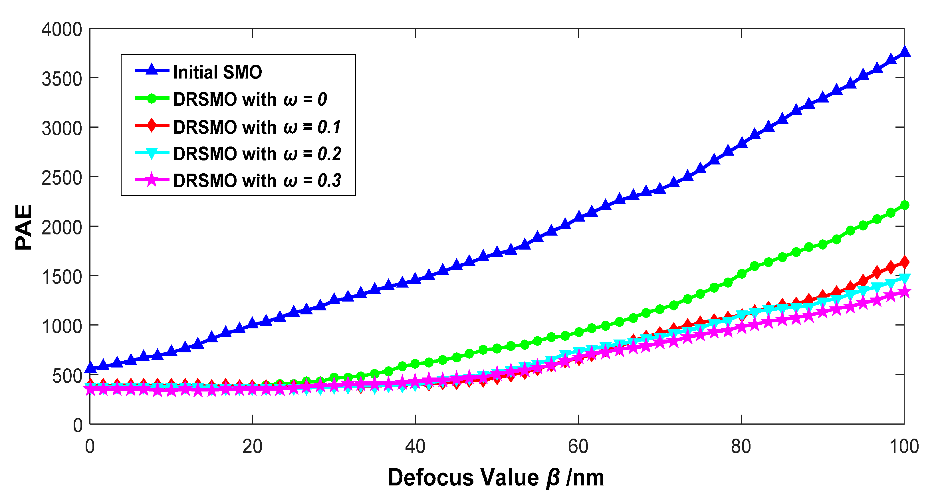
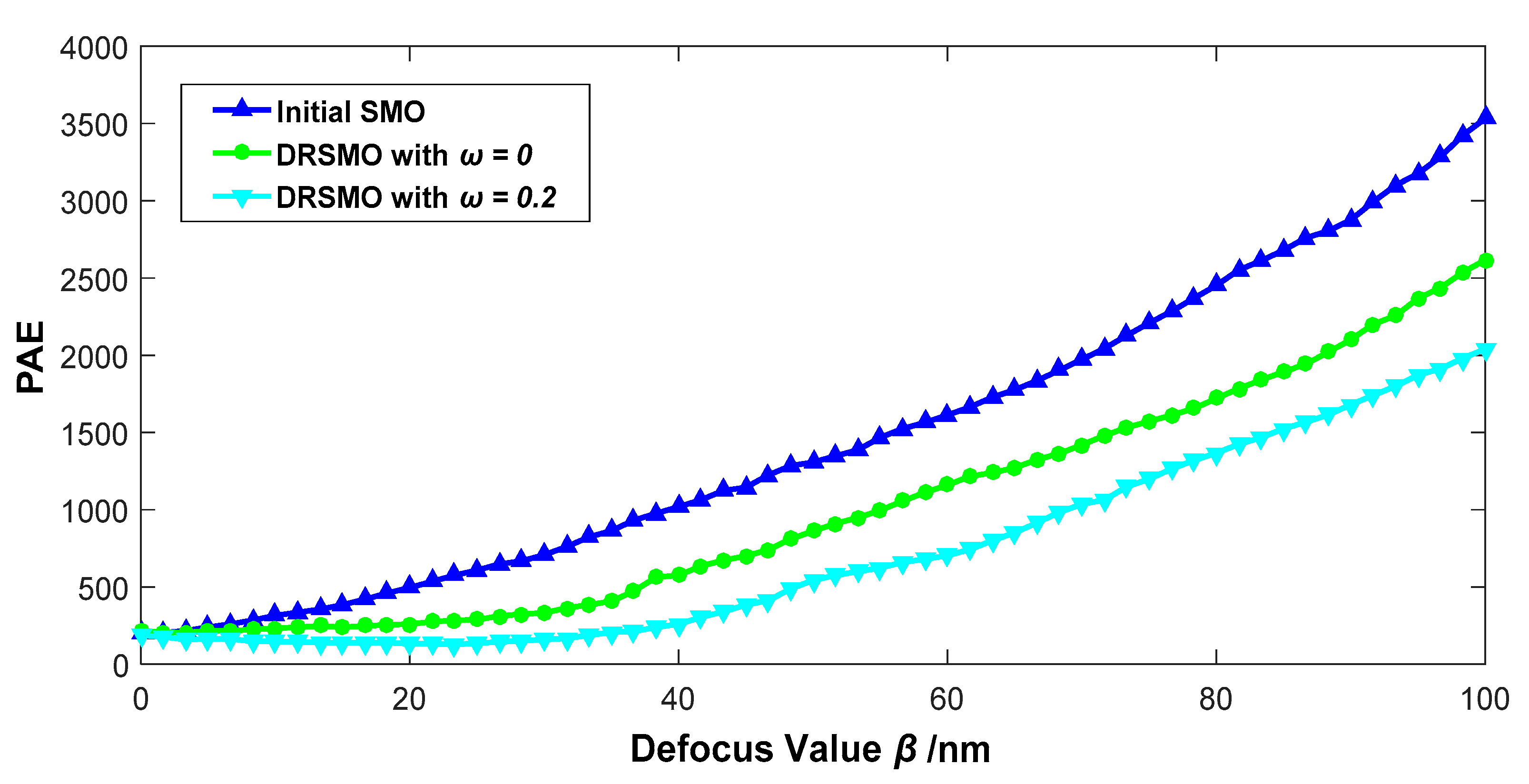
To further prove a robust improvement, Figure 4 depicts the defocus–PAE curves in the evaluation range of 0–100 nm for target 1 optimized systems. It should be noted that each weight factor ω corresponds to a set of optimized source and mask. The slope of each curve reflected the process robustness, and a lower slope meant lower sensitivity for the optimized systems to focus on shifting. It should be noted that the slope of each curve gradual decreased in the order of initial SMO (blue curve), DRSMO with ω = 0 (green curve), DRSMO with ω = 0.1 (red curve), DRSMO with ω = 0.2 (azury curve), and DRSMO with ω = 0.3 (purple curve). We concluded that DRSMO is beneficial to reduce defocusing sensitivity and to gain a more uniform exposure pattern within a long range of defocusing, which means a better system robustness against uncertain and changeable focus shifts in a real lithography process. The core idea of the DRSMO is to introduce the defocusing sensitivity to constrain the uniformity of printed patterns in different defocus variations. Thus, simulations further compare the optimization performance of DRSMO, which merely operate at the fidelity part (ω = 0) and DRSMO driven by the sensitivity penalty (ω ≠ 0). For instance, comparing the DRSMO with ω = 0 (green curve) and DRSMO with ω = 0.1 (red curve) in Figure 4, the slope of the red curve is lower than that of the green curve, which infers that the introduction of the sensitivity penalty can further improve pattern uniformity with a wide range of defocus variations. It was proved that the validity of introduction sensitivity penalty further improves the optimization performance. In brief, to maximize the DRSMO optimization performance, both the fidelity part and the penalty term must be introduced into the optimization framework, and the weight factor ω must be chosen appropriately.
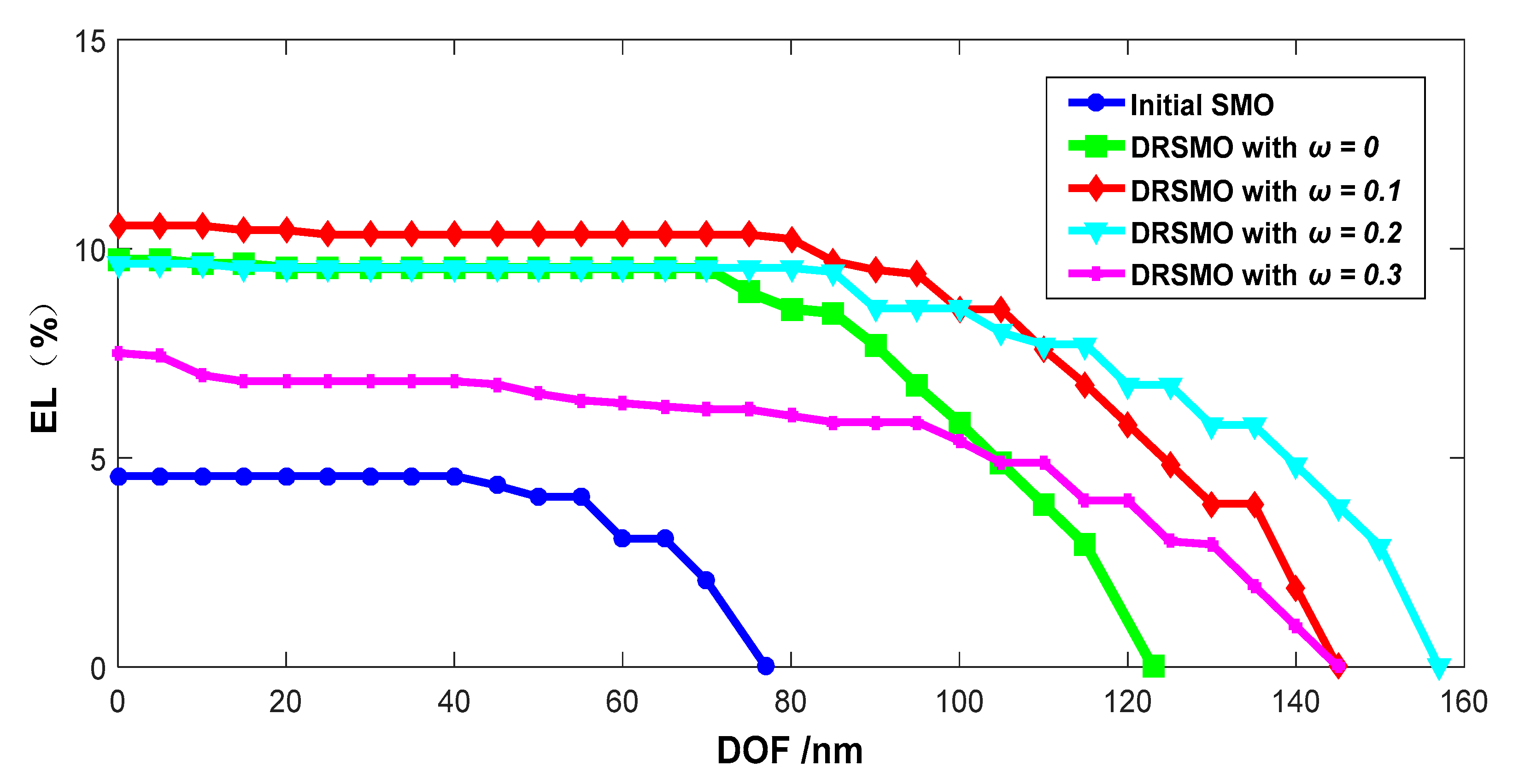
In actual lithography processes, PW is one of the critical evaluation criteria which refers to the exposure error tolerance. Figure 5 shows the PWs for the conventional SMO (blue curve), the DRSMO with the weight factor ω = 0 (green curve), ω = 0.1 (red curve), ω = 0.2 (azury curve), and ω = 0.3 (purple curve). It is illustrated that the PW of the proposed DRSMO was evidently larger than that of the initial SMO. For the initial SMO, the maximal EL was less than 5%, which was far below the actual exposure requirements. By using DRSMO, the EL maximal increased from 4.5% to 10.5%. Similar results were found when comparing the difference of DRSMO without the sensitive penalty and DRSMO with the sensitive penalty. For example, when comparing PW with ω = 0 (green curve) and ω = 0.1 (red curve), a wider PW was found for the red curve than the green curve. It is inferred that the sensitive penalty is helpful for improving system robustness so that it indirectly boosts PW. However, because the cost function does not involve terms which directly relate to EL and DOF, the relationship between weight factor ω and PW is uncertain and unclear. In this way, although DRSMO with ω = 0.3 had the best defocus robustness, the PW was shrunk because the weight factor was too large that it led to overfitting during the training process. This illustrates that a well-chosen weight factor ω is important to simultaneously improve robustness and PW.
Table 2 summarizes the target 1 comparison of optimization results for conventional SMO, DRSMO with ω = 0, ω = 0.1, ω = 0.2, and ω = 0.3, respectively. It should be noted that PAE sensitivity factor Sβ declined significantly with the ω increase. Compare with initial SMO, the largest decrease of in DRSMO with ω = 0.3 is 63.5%. Integrated consider the improvement of both and PW, ω = 0.1 is a relative reasonable weight factor for maximize optimization performance.
Target 2 consisted of a series of vertical and horizontal mixed lines. Figure 6 shows the defocus–PAE curves in the evaluation range of (0 nm, 100 nm) for target 2; optimizations were proceeded by the MBGD algorithm. It should be noted that the slope of the DRSMO with a ω = 0.2 (azury curve) lower than that of DRSMO with a ω = 0 (green curve) and initial SMO (blue curve) proved the effectiveness of the sensitivity penalty.
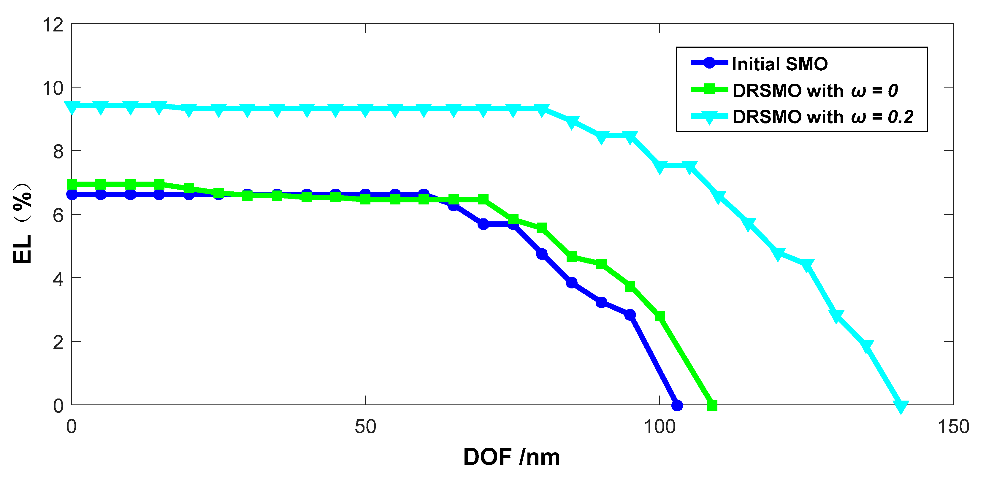
Meanwhile, the improvement of PW for target 2 was still apparent for the DRSMO approach. Figure 7 shows the PWs for the initial SMO (blue curve) and the DRSMO with the weight factors ω = 0 (green curve) and ω = 0.2 (azury curve). It should be noted that the PW had no significant improvement for the DRSMO with ω = 0 compared to the initial SMO, but due to the lower defocus sensitivity, the PW of the DRSMO with ω = 0.2 was enlarged. It was apparent that the introduction of the sensitivity penalty was beneficial for further improvement of the PW. Similarly, Table 3 summarizes the comparison of the target 2 optimization results for the initial SMO and DRSMO with ω = 0 and ω = 0.2, respectively. It shows that the DOF corresponding to EL = 5% maximally increased by 54.5%.
3.3. Comparison of SGD and MBGD Algorithm for DRSMO
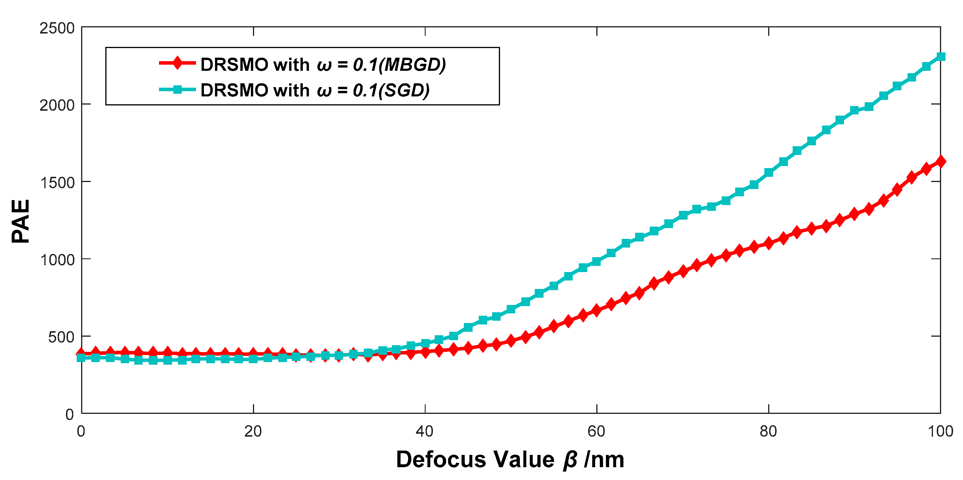
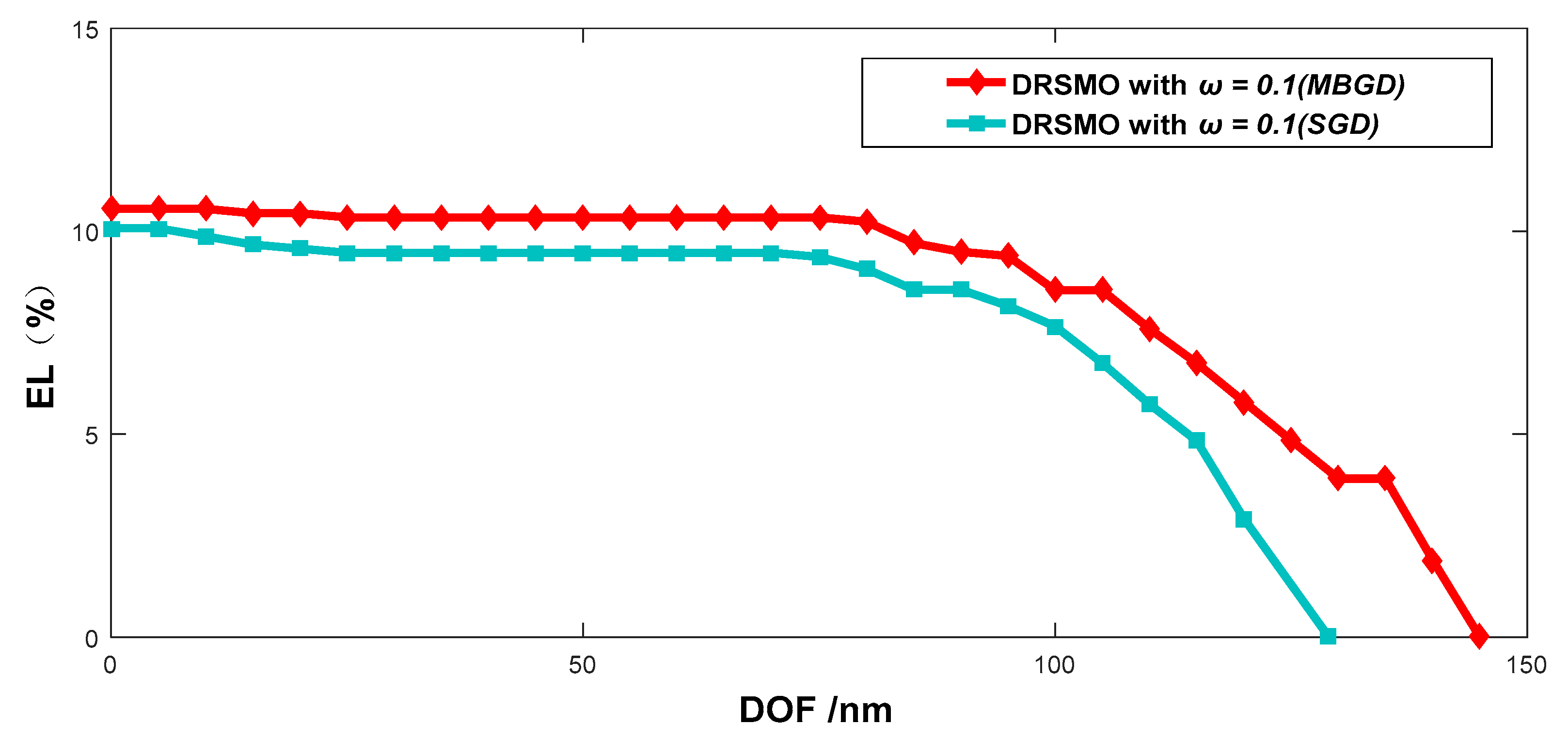
We have previously used the SGD algorithm to solve multi-objective SMO [25,26] and it converged well with fast speed. However, due to the wider sampling range of defocusing in the DRSMO framework, it was hard for the SGD algorithm to search for the global optimal direction if each iteration was only driven by one sample gradient in the training set. To compare the SGD and MBGD optimization performance for the DRSMO in terms of speed and accuracy, we generated the same training set with 900 sample points for both MBGD and SGD optimization processes (for the MBGD algorithm, there were a total of three samples per iteration and 300 iterations. For the SGD algorithm, there was a total of one sample per iteration and 900 iterations). Figure 8 illustrates that the defocus–PAE curves for target 1 optimization in the case of the same weight factor, ω = 0.1, was proceeded by the SGD and MBGD algorithms, respectively. It was demonstrated that the slope of the DRSMO was proceeded by the MBGD (red curve), which was lower than that of the SGD (jasper curve). It indicates the better optimization performance for the MBGD in the same training set. Similarly, Figure 9 shows that the PWs with the same weight factor were proceeded by the SGD and MBGD algorithms, respectively. It was the MBGD algorithm that provided a wider PW due to the lower defocus sensitivity.
Table 4 summarizes the comparison of the optimization performances for target 1 proceeded by the MBGD and SGD, respectively. It clearly shows that the lower Sβ and larger DOF were improved by MBGD optimization. Meanwhile, Table 4 shows the comparison of run times, although SGD had a relatively weak optimization performance but was faster in regard to convergence rates. In addition, all computations were carried out on a server with an Intel core i5 8400 CPU, 2.8GHz, 16.0 GB of RAM.
In conclusion, both the MBGD and SGD were beneficial for improving DOF and PW. However, the massive samples taken from the defocusing disturbances made it hard for the SGD to converge to a global search direction. Therefore, the MBGD algorithm was applied to the DRSMO multi-objective optimization problem most effectively.
4. Conclusions
In conclusion, we proposed the DRSMO to compensate for uncertain defocus and OPE in real lithography processes. The inverse optimization framework was based on a new cost function that constrained the uniformity of an aerial image in different defocus disturbances, and a more robust lithographic source and mask with lower defocus sensitivities were designed. Using this method, the robustness against focus shifting was dramatically improved and the DOF and PW were extremely enlarged as well. It created a larger exposure tolerance in the actual lithography process and it was especially applied to high fidelity exposures in cutting-edge technical nodes.
Author Contributions
Conceptualization, P.W. and Y.L.; methodology, P.W. and T.L.; software, P.W. and T.L.; validation, P.W. and T.L.; formal analysis, N.S. and Y.L.; investigation, P.W. and T.L.; resources, T.L.; data curation, N.S. and Y.S.; writing—original draft preparation, P.W. and Y.L.; writing—review and editing, P.W. and Y.L.; visualization, E.L. and Y.S.; supervision, Y.L.; project administration, Y.L.; funding acquisition, Y.L.
Funding
This research was funded by the General Program of National Natural Science Foundation of China (Grant No.61675026) and the National Science and Technology Major Project (Grant No. 2017ZX02101006-001).
Acknowledgments
We gratefully acknowledge KLA-Tencor Corporation for providing academic use of PROLITH. We thank Mentor Graphics Corporation for providing academic use of Calibre.
Conflicts of Interest
The authors declare no conflict interest.
Appendix A
For brevity, Equation (2), can be simplified as:
where
Similarly, according to our previous work [16], can also be simplified as:
where is the mask layout, is the mask diffraction matrix, and is the transfer function of the project lens.
Then, discretize the sensitivity penalty in each defocus disturbance . Based on the chain rule, according to Equations (6) and (A1), the analytical sensitivity penalty can be expressed as:
where represents the m and nth sampling point in the aerial image matrix , and represents the r and sth sampling point in matrix as well. Details of , and can be formulated as:
and
Appendix B
In order to reduce the bound-constrained source and mask optimization problem, we apply parametric transformation to realize unconstrained optimization such that [16]
Through this transformation, the entry values of can be enlarged in the range of (−∞, ∞). According to Equations (A5) and (A9), the gradient of Yi to the source parameters is
Thus, simplify the matrix of Equation (A10) to form
where is the one-valued vector.
Similarly, according to Equations (A5) and (A9), the gradient of to the mask parameters can be formulated as
Thus, simplify the matrix to form
where o rotates the matrix in the argument by 180°, and * is the conjugate operator, respectively. For brevity in the description, we simplified the above terms , , , , and can be expanded
Appendix C
Discretize the fidelity part in each defocus disturbance. Actually, each gradient of fidelity part has already been derived in our previous work [16], the gradient of to the source parameters is
Thus, simplify the matrix to form
Likewise, the gradient of Fi to the mask parameters
is
where .
References
- Fujisawa, T.; Asano, M.; Sutani, T.; Inoue, S.; Yamada, H.; Sugamoto, J.; Okumura, K.; Hagiwara, T.; Oka, S. Wafer flatness for CD control in photolithography. In Proceedings of the SPIE’s 27th Annual International Symposium on Microlithography, Santa Clara, CA, USA, 3–8 March 2002; Volume 4691. [Google Scholar]
- Mao, Y.; Li, S.; Sun, G.; Wang, J.; Duan, L.; Bu, Y.; Wang, X. The thermal aberration analysis of a lithography projection lens. In Proceedings of the SPIE Advanced Lithography, San Jose, CA, USA, 26 February–2 March 2017; Volume 10147. [Google Scholar]
- Khounsary, A.M.; Chojnowski, D.; Mancini, D.C.; Lai, B.P.; Dejus, R.J. Thermal management of masks for deep x-ray lithography. In Proceedings of the Optical Science, Engineering and Instrumentation ’97, San Diego, CA, USA, 27 July–1 August 1997; Volume 3151. [Google Scholar]
- Azpiroz, J.T.; Rosenbluth, A.E. Impact of Sub-Wavelength Electromagnetic Diffraction in Optical Lithography for Semiconductor Chip Manufacturing; IEEE: New York, NY, USA, 2013. [Google Scholar]
- Rosenbluth, A.E.; Bukofsky, S.; Hibbs, M.; Lai, K.F.; Molless, A.; Singh, R.N.; Wong, A. Optimum mask and source patterns to print a given shape. In Optical Microlithography XIV, Pts 1 and 2; Progler, C.J., Ed.; Spie-Int Soc Optical Engineering: Bellingham, WA, USA, 2001; Volume 4346, pp. 486–502. [Google Scholar]
- Ma, X.; Arce, G.R. Pixel-based OPC optimization based on conjugate gradients. Opt. Express 2011, 19, 2165–2180. [Google Scholar] [CrossRef] [PubMed]
- Ma, X.; Arce, G.R. Pixel-based simultaneous source and mask optimization for resolution enhancement in optical lithography. Opt. Express 2009, 17, 5783–5793. [Google Scholar] [CrossRef] [PubMed]
- Ma, X.; Han, C.Y.; Li, Y.Q.; Dong, L.S.; Arce, G.R. Pixelated source and mask optimization for immersion lithography. J. Opt. Soc. Am. A-Opt. Image Sci. Vis. 2013, 30, 112–123. [Google Scholar] [CrossRef] [PubMed]
- Yu, J.C.; Yu, P.C. Gradient-Based Fast Source Mask Optimization (SMO). In Optical Microlithography XXIV; Dusa, M.V., Ed.; Spie-Int Soc Optical Engineering: Bellingham, WA, USA, 2011; Volume 7973. [Google Scholar]
- Yu, P.; Pan, D.Z.; Mack, C.A. Fast lithography simulation under focus variations for OPC and layout optimizations. In Design and Process Integration for Microelectronic Manufacturing IV; Wong, A.K.K., Singh, V.K., Eds.; Spie-Int Soc Optical Engineering: Bellingham, WA, USA, 2006; Volume 6156. [Google Scholar]
- Yu, P.; Shi, S.X.; Pan, D.Z. True process variation aware optical proximity correction with variational lithography modeling and model calibration. J. Micro-Nanolithogr. MEMS MOEMS 2007, 6, 574–576. [Google Scholar] [CrossRef]
- Guo, X.J.; Li, Y.Q.; Dong, L.S.; Liu, L.H.; Ma, X.; Han, C.Y. Parametric source-mask-numerical aperture co-optimization for immersion lithography. J. Micro-Nanolithogr. MEMS MOEMS 2014, 13, 043013. [Google Scholar] [CrossRef] [Green Version]
- Sheng, N.; Li, E.; Sun, Y.; Li, T.; Li, Y.; Wei, P.; Liu, L. Mitigating the Impact of Mask Absorber Error on Lithographic Performance by Lithography System Holistic Optimization. Appl. Sci. 2019, 9, 1275. [Google Scholar] [CrossRef]
- Peng, Y.; Zhang, J.Y.; Wang, Y.; Yu, Z.P. Gradient-Based Source and Mask Optimization in Optical Lithography. IEEE Trans. Image Process. 2011, 20, 2856–2864. [Google Scholar] [CrossRef] [PubMed]
- Ma, X.; Li, Y.Q.; Guo, X.J.; Dong, L.S. Robust Resolution Enhancement Optimization Methods to Process Variations based on Vector Imaging Model. In Optical Microlithography XXV, Pts 1and 2; Conley, W., Ed.; Spie-Int Soc Optical Engineering: Bellingham, WA, USA, 2012; Volume 8326. [Google Scholar]
- Ma, X.; Li, Y.Q.; Guo, X.J.; Dong, L.S.; Arce, G.R. Vectorial mask optimization methods for robust optical lithography. J. Micro-Nanolithogr. MEMS MOEMS 2012, 11, 043008. [Google Scholar] [CrossRef]
- Jia, N.; Lam, E.Y. Machine learning for inverse lithography: Using stochastic gradient descent for robust photomask synthesis. J. Opt. 2010, 12. [Google Scholar] [CrossRef]
- Jia, N.N.; Lam, E.Y. Pixelated source mask optimization for process robustness in optical lithography. Opt. Express 2011, 19, 19384–19398. [Google Scholar] [CrossRef] [PubMed] [Green Version]
- Jia, N.N.; Wong, A.K.; Lam, E.Y. Robust Mask Design with Defocus Variation Using Inverse Synthesis. In Lithography Asia 2008; Chen, A.C., Lin, B., Yen, A., Eds.; Spie-Int Soc Optical Engineering: Bellingham, WA, USA, 2008; Volume 7140. [Google Scholar]
- Li, S.K.; Wang, X.Z.; Bu, Y. Robust pixel-based source and mask optimization for inverse lithography. Opt. Laser Technol. 2013, 45, 285–293. [Google Scholar] [CrossRef]
- Shen, Y.J.; Jia, N.N.; Wong, N.; Lam, E.Y. Robust level-set-based inverse lithography. Opt. Express 2011, 19, 5511–5521. [Google Scholar] [CrossRef] [PubMed] [Green Version]
- Gallatin, G.M. High-numerical-aperture scalar imaging. Appl. Opt. 2001, 40, 4958–4964. [Google Scholar] [CrossRef] [PubMed]
- Mack, C. Fundamental Principles of Optical Lithography: The Science of Microfabrication; Wiley: Hoboken, NJ, USA, 2007; pp. 265–276. [Google Scholar]
- Ma, X.; Arce, G. Binary mask optimization for inverse lithography with partially coherent illumination. J. Opt. Soc. Am. A-Opt. Image Sci. Vis. 2008, 25, 2960–2970. [Google Scholar] [CrossRef] [PubMed]
- Han, C.Y.; Li, Y.Q.; Ma, X.; Liu, L.H. Robust hybrid source and mask optimization to lithography source blur and flare. Appl. Opt. 2015, 54, 5291–5302. [Google Scholar] [CrossRef] [PubMed]
- Li, T.; Li, Y.Q. Lithographic Source and Mask Optimization with Low Aberration Sensitivity. IEEE Trans. Nanotechnol. 2017, 16, 1099–1105. [Google Scholar] [CrossRef]
- Li, M.; Zhang, T.; Chen, Y.; Smola, A.J. Efficient mini-batch training for stochastic optimization. In Proceedings of the 20th ACM SIGKDD International Conference on Knowledge Discovery and Data Mining—KDD ’14, New York, NY, USA, 24–27 August 2014; pp. 661–670. [Google Scholar]
Figure 1.
Forward calculation and inverse optimization process for defocus robust SMO (DRSMO).

Figure 2.
Two test patterns used in the simulation: (a) Test pattern 1; (b) Test pattern 2. The PW calculation positions are marked at the yellow lines.
Figure 2.
Two test patterns used in the simulation: (a) Test pattern 1; (b) Test pattern 2. The PW calculation positions are marked at the yellow lines.

Figure 3.
Target 2 simulation results of the initial SMO, SMO under assigned focus plane (100 nm defocusing), and DRSMO with ω = 0.2, respectively.
Figure 3.
Target 2 simulation results of the initial SMO, SMO under assigned focus plane (100 nm defocusing), and DRSMO with ω = 0.2, respectively.

Figure 4.
The defocus–pattern error (PAE) curves of target 1 for initial SMO (blue curve), the DRSMO with the weight factor ω = 0 (green curve), ω = 0.1 (red curve), ω = 0.2 (azury curve), and ω = 0.3 (purple curve). Optimizations were proceeded by the MBGD algorithm.
Figure 4.
The defocus–pattern error (PAE) curves of target 1 for initial SMO (blue curve), the DRSMO with the weight factor ω = 0 (green curve), ω = 0.1 (red curve), ω = 0.2 (azury curve), and ω = 0.3 (purple curve). Optimizations were proceeded by the MBGD algorithm.

Figure 5.
Process window (PW) of target 1 for the initial SMO (blue curve), the DRSMO with the weight factor ω = 0 (green curve), ω = 0.1 (red curve), ω = 0.2 (azury curve), and ω = 0.3 (purple curve). Optimizations were proceeded by the MBGD algorithm.
Figure 5.
Process window (PW) of target 1 for the initial SMO (blue curve), the DRSMO with the weight factor ω = 0 (green curve), ω = 0.1 (red curve), ω = 0.2 (azury curve), and ω = 0.3 (purple curve). Optimizations were proceeded by the MBGD algorithm.

Figure 6.
The defocus–PAE curves of target 2 for initial SMO (blue curve), the DRSMO with the weight factor ω = 0 (green curve) and ω = 0.2 (azury curve), respectively. Optimizations were proceeded by the MBGD algorithm.
Figure 6.
The defocus–PAE curves of target 2 for initial SMO (blue curve), the DRSMO with the weight factor ω = 0 (green curve) and ω = 0.2 (azury curve), respectively. Optimizations were proceeded by the MBGD algorithm.

Figure 7.
PWs of target 2 for the initial SMO (blue curve) and the DRSMO with the weight factors ω = 0 (green curve) and ω = 0.2 (azury curve), respectively. Optimizations were proceeded by the MBGD algorithm.
Figure 7.
PWs of target 2 for the initial SMO (blue curve) and the DRSMO with the weight factors ω = 0 (green curve) and ω = 0.2 (azury curve), respectively. Optimizations were proceeded by the MBGD algorithm.

Figure 8.
The defocus–PAE curves of target 1 for the DRSMO with the same weight factor ω = 0.1 which was proceeded by the SGD algorithm (jasper curve) and MBGD algorithms (red curve), respectively.
Figure 8.
The defocus–PAE curves of target 1 for the DRSMO with the same weight factor ω = 0.1 which was proceeded by the SGD algorithm (jasper curve) and MBGD algorithms (red curve), respectively.

Figure 9.
PWs of target 1 for the DRSMO with the same weight factor ω = 0.1 that were proceeded by the SGD algorithm (jasper curve) and MBGD algorithms (red curve), respectively.
Figure 9.
PWs of target 1 for the DRSMO with the same weight factor ω = 0.1 that were proceeded by the SGD algorithm (jasper curve) and MBGD algorithms (red curve), respectively.


Table 1.
Stochastic gradient descent (SGD) and mini-batch gradient descent (MBGD) optimization procedure.
Table 1.
Stochastic gradient descent (SGD) and mini-batch gradient descent (MBGD) optimization procedure.
| SGD procedure |
| 1. Initialization: Assign the starting source parameter , mask parameter , the source step size , the mask step size , the upper limit iteration number 2. Optimization: Simultaneously update the source and mask patterns: While Calculate the generate , , respectively; Update the source and mask parameters end 3. Output: the optimized source and mask parameters. |
| MBGD procedure |
| 1. Initialization: Assign the starting source parameter mask parameter , the source step size , the mask step size , the upper limit iteration number , the batch number 2. Optimization: Simultaneously update the source and mask patterns: While Random generate a set of the defocus values Calculate the corresponding gradient of cost function , respectively; Update the source and mask parameters end 3. Output: the optimized source and mask parameters. |
Table 2.
The target 1 optimized values of Sβ, depth of focus (DOF) (nm) corresponding to exposure latitude (El) equal to 5% and 8% for conventional SMO, and DRSMO with ω = 0, ω = 0.1, ω = 0.2, and ω = 0.3, respectively.
Table 2.
The target 1 optimized values of Sβ, depth of focus (DOF) (nm) corresponding to exposure latitude (El) equal to 5% and 8% for conventional SMO, and DRSMO with ω = 0, ω = 0.1, ω = 0.2, and ω = 0.3, respectively.
| Method | Sβ | DOF (EL = 5%) | DOF (EL = 8%) |
|---|---|---|---|
| Initial SMO | 56.1 | 0 | 0 |
| DRSMO (ω = 0) | 36.6 | 102 | 87 |
| DRSMO (ω = 0.1) | 25.5 | 122 | 107 |
| DRSMO (ω = 0.2) | 23.8 | 138 | 105 |
| DRSMO (ω = 0.3) | 20.5 | 102 | 0 |
Table 3.
The target 2 optimized values of Sβ, DOF (nm) corresponding to ELs equal to 5% and 8% for the conventional SMO, and DRSMO with ω = 0, ω = 0.1, ω = 0.2, and ω = 0.3, respectively.
Table 3.
The target 2 optimized values of Sβ, DOF (nm) corresponding to ELs equal to 5% and 8% for the conventional SMO, and DRSMO with ω = 0, ω = 0.1, ω = 0.2, and ω = 0.3, respectively.
| Method | Sβ | DOF (EL = 5%) | DOF (EL = 8%) |
|---|---|---|---|
| Initial SMO | 54.2 | 77 | 0 |
| DRSMO (ω = 0) | 40.3 | 82 | 0 |
| DRSMO (ω = 0.2) | 32.6 | 119 | 97 |
Table 4.
The values of Sβ, DOF (nm) corresponding to ELs equal to 5% and 8% and run time (seconds) for DRSMO proceeded by the MBGD and SGD, respectively.
Table 4.
The values of Sβ, DOF (nm) corresponding to ELs equal to 5% and 8% and run time (seconds) for DRSMO proceeded by the MBGD and SGD, respectively.
| Algorithm | Sβ | DOF (EL = 5%) | DOF (EL = 8%) | Run Time | |
|---|---|---|---|---|---|
| DRSMO (ω = 0.1) | MBGD | 25.5 | 122 | 107 | 22,072.7 |
| SGD | 34.3 | 111 | 92 | 14,846.5 |
© 2019 by the authors. Licensee MDPI, Basel, Switzerland. This article is an open access article distributed under the terms and conditions of the Creative Commons Attribution (CC BY) license (http://creativecommons.org/licenses/by/4.0/).
Share and Cite
MDPI and ACS Style
Wei, P.; Li, Y.; Li, T.; Sheng, N.; Li, E.; Sun, Y. Multi-Objective Defocus Robust Source and Mask Optimization Using Sensitive Penalty. Appl. Sci. 2019, 9, 2151. https://doi.org/10.3390/app9102151
AMA Style
Wei P, Li Y, Li T, Sheng N, Li E, Sun Y. Multi-Objective Defocus Robust Source and Mask Optimization Using Sensitive Penalty. Applied Sciences. 2019; 9(10):2151. https://doi.org/10.3390/app9102151
Chicago/Turabian StyleWei, Pengzhi, Yanqiu Li, Tie Li, Naiyuan Sheng, Enze Li, and Yiyu Sun. 2019. "Multi-Objective Defocus Robust Source and Mask Optimization Using Sensitive Penalty" Applied Sciences 9, no. 10: 2151. https://doi.org/10.3390/app9102151
Note that from the first issue of 2016, this journal uses article numbers instead of page numbers. See further details here.