Neurofitter: A parameter tuning package for a wide range of electrophysiological neuron models
- 1 Theoretical Neurobiology, University of Antwerp, Belgium
- 2 Computational Neuroscience Unit, Okinawa Institute of Science and Technology, Japan
- 3 Volen Center for Complex System, Brandeis University, USA
The increase in available computational power and the higher quality of experimental recordings have turned the tuning of neuron model parameters into a problem that can be solved by automatic global optimization algorithms. Neurofitter is a software tool that interfaces existing neural simulation software and sophisticated optimization algorithms with a new way to compute the error measure. This error measure represents how well a given parameter set is able to reproduce the experimental data. It is based on the phase-plane trajectory density method, which is insensitive to small phase differences between model and data. Neurofitter enables the effortless combination of many different time-dependent data traces into the error measure, allowing the neuroscientist to focus on what are the seminal properties of the model.
We show results obtained by applying Neurofitter to a simple single compartmental model and a complex multi-compartmental Purkinje cell (PC) model. These examples show that the method is able to solve a variety of tuning problems and demonstrate details of its practical application.
Introduction
One of the big challenges facing a scientist developing a detailed computational model is how to tune model parameters that cannot be directly derived from experimental results. This is especially true for neuroscientists who develop complex models of neurons that consist of many different compartments (Rall, 1964 ) incorporating multiple types of voltage-gated ion channels (London and Häusser 2005 ) that all require separate parameters. This problem can become even more complicated when one wants to model neuronal networks, which can consist of a large number of neurons of different types (De Schutter et al., 2005 ). Because of the sharp increase in computational power that is made available to scientists in the field (Markram, 2006 ) and because of the increasingly detailed knowledge of neuronal mechanisms that underlie neuronal function, these models have become more and more complex, causing an increase in the number of parameters that need to be fitted. In the extreme case there can be different parameters for each compartment or neuron.
In the ideal situation, the values for every parameter of a model are obtained from the same set of experimental data (Rall et al., 1992 ), but unfortunately this is not always possible. First, it can be difficult to obtain some parameters within an acceptable error margin. For example, reliable kinetic data for ion channels that generate small currents are hard to extract. A second problem to be avoided is the “failure of averaging”. Sometimes the parameter space containing the best maximal conductances for voltage-gated channels is very concave, excluding the mean. So the general practice of calculating the mean value from experiments on different cells is not guaranteed to provide good values (De Schutter and Bower, 1994 ; Golowasch et al., 2002 ).
Until recently the traditional approach was to tune neuronal model parameters by hand. This requires a lot of effort and knowledge from the scientist and can be very challenging since the underlying mechanisms are highly non-linear and difficult to grasp. It can also induce some bias as the scientist has a natural tendency to assign in advance different roles to each parameter. However, complicated models have been successfully developed this way (De Schutter and Bower, 1994 ; Traub et al., 1991 ).
Several parameter search methods have been developed over the years to automate the tuning of neuron models. Three different approaches can be distinguished. First, some methods do a brute force scan of the entire parameter space (Bhalla and Bower, 1993 ; Foster et al., 1993 ; Prinz et al., 2003 ). Most methods tune the model by use of Monte Carlo optimization algorithms, including genetic algorithms and simulated annealing (Achard and De Schutter, 2006 ; Baldi et al., 1998 ; Bush et al., 2005 ; Gerken et al., 2006 ; Keren et al., 2005 ; Schneider et al., 2004 ; Vanier and Bower, 1999 ; Weaver and Wearne, 2006 ). Finally, recent approaches use mathematical techniques to infer in a more direct way values for the model parameters (Huys et al., 2006 ).
Because of international initiatives (Bjaalie and Grillner, 2007 ), experimentalists are increasingly sharing their data with modelers, and many modelers make their model simulation codes available in databases like ModelDB (Hines et al., 2004 ). This makes it possible for people from both parts of the field to interact with each other and to generate models that reproduce the available experimental data as closely as possible.
In this paper, we present a command-line software tool for automated parameter searches, called Neurofitter. The innovative part of Neurofitter is the use of the phase-plane trajectory density method (LeMasson and Maex, 2001 ) to measure how faithfully the model can reproduce experimental data. The users provide the experimental data in the form of time-dependent traces, specify the model code written for any neuron simulator environment and select an optimization technique from a library of third-party routines. Subsequently, Neurofitter will run the model with different sets of parameters and try to find an optimal model based on the target data.
Software Description and Methods
General algorithm
Neurofitter is aimed to rapidly find the best possible parameter set of a neuron model to replicate given experimental data. It requires a function that quantifies the goodness of a parameter set. That way, different parameter sets can be ranked and the best of them selected. The core task performed by Neurofitter is therefore the computation of an error function that connects every parameter set of a neuron model with a single value that represents how well these parameters are able to replicate the experimental data.
The user has to provide both the experimental data and a computational neuron model that can be run with different parameter sets. All the settings of Neurofitter are defined in an XML file provided to the software during startup. Figure 1 gives a general overview of the operations performed by Neurofitter, which are listed in more detail in Appendix A, while Figure 2 provides an overview of the underlying software structure and its relation to other software packages.
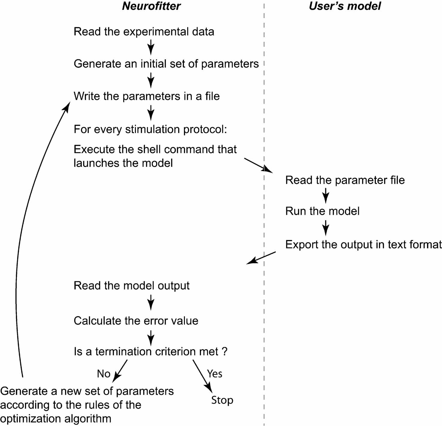
Figure 1. General algorithm. Short description of the core operations of the algorithm. The left panel contains the steps performed by Neurofitter; the right panel the actions the user has to implement in the neuron model code.
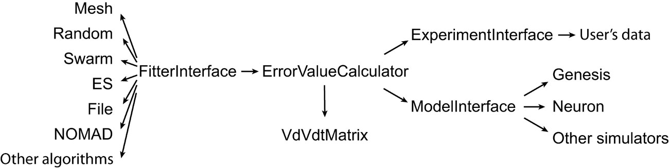
Figure 2. General structure. Schema describing the most important abstract C++ classes implemented in Neurofitter. An arrow represents the relationship “makes use of”.
First, Neurofitter will analyze the experimental data (see Section Experimental Data Format) and store it in an object ExperimentInterface so that it can be compared to model traces.
An object ModelInterface is created that provides an interface with the model. This object creates model output traces contained in DataTrace objects, one for every stimulation protocol, by causing a simulator to run the user-provided model (see Section Adapting the Model Code) with a set of parameters.
Next, the ModelInterface and ExperimentInterface objects are passed to a ErrorValueCalculator that creates VdVdtMatrix objects from the model and experiment Datatraces using the phase-plane trajectory density method (see Section The Error Function). The ErrorValueCalculator calculates an error value for each set of parameters, and will store this information in a file.
Finally, the optimization algorithm (see Section Optimization Algorithms) is run using a FitterInterface object. FitterInterface makes use of ErrorValueCalculator that represents the error function. Neurofitter runs until a termination criterion of the optimization algorithm is reached and returns the best set of parameters found.
Experimental data format
The experimental data has to consist of time-dependent traces that may have been recorded from different sites in the neuron, applying different stimulation protocols or recording methods. The user should be careful when combining data from different experiments or sources (De Schutte rand Steuber, 2000 ) as no model may be able to fit a disjoint set.
The data is submitted as a set of ASCII files (see Figure 3 ), which should all have the same sampling rate. There has to be one file for each separate model run used in the evaluation (corresponding to different experimental protocols) and for every recording method (e.g., a voltage or a calcium concentration recording). For a more detailed explanation of the data format used, refer to Appendix B.
Adapting the model code
Neurofitter is able to interface with different neural simulator packages. We have written specialized interfaces with the GENESIS (Bower and Beeman, 1998 ) and NEURON (Hines and Carnevale, 1997 ) simulators. It is possible to use other software packages to simulate the neuron model, provided the model can be started up from a shell command. The simulator must read the parameters it has to use from a file before model execution and write output to another file.
The user has to adapt a model script slightly to enable it to communicate with Neurofitter. The parameter values that need to be tuned should no longer be defined as constants in the model, but should be read from a file provided by Neurofitter. Every time the optimization algorithm wants to evaluate a point in the parameters space, Neurofitter creates a file at a fixed location (which is specified in the XML settings). This file contains the run parameters (for example amplitude and location of current injection), the model parameters (e.g., the ion channel maximal conductances) and the name and location of the file to which the model should write its output. Next the neuron simulator is executed by a shell command. At this point the model code should read the file that was created by Neurofitter, run the model and write its output to the correct file location in the same format as the experimental data.
The output trace of the model has to have the same (fixed) sampling rate as the experimental data and this rate has to be specified in the XML settings file. If Neurofitter is used with the variable time step methods available in some neuron simulators, care should be taken that output is generated at the fixed sampling rate.
Neurofitter settings
The settings for the software are specified in an XML file (Figure 4 ) that contains sections for each of the different settings, namely FitterParameters, TraceReaderParameters, ModelParameters, ExperimentParameters, ErrorValueCalculatorParameters. At present this XML file must be made or adapted by the user but future versions of Neurofitter will provide a graphical interface to generate the XML file.
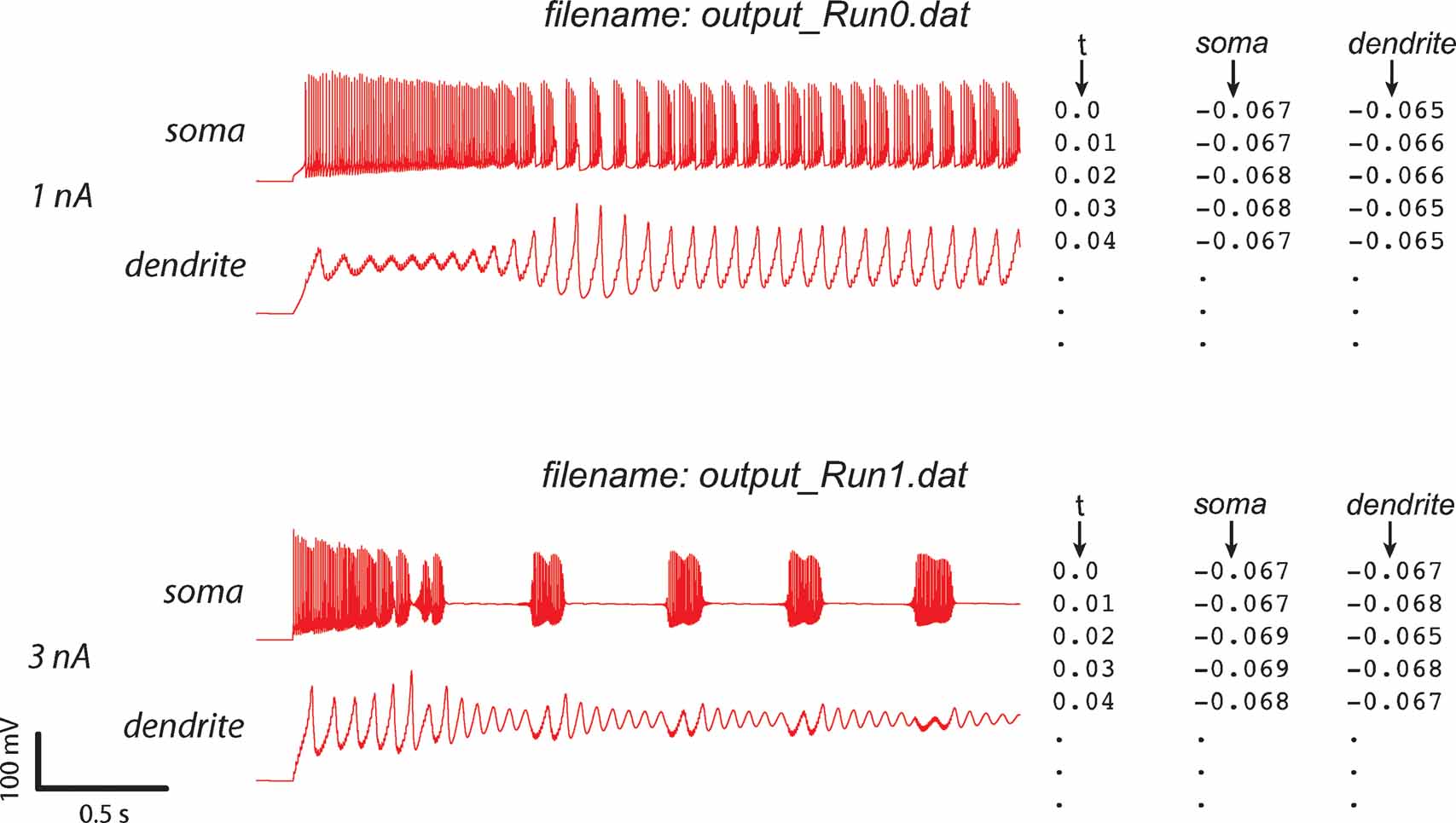
Figure 3. Experimental data format. The format of the ASCII experimental files is shown (right) with the corresponding data traces (left). If the experiment consists of a recording at two sites, with two different consecutive injections (current amplitudes 1 and 3 nA), two files should be created output_Run0.dat and output_Run1.dat, each containing one column with the timestamps and two columns with the recorded data (V) in soma and dendrite. Example was made using the PC model (De Schutter and Bower, 1994 ).
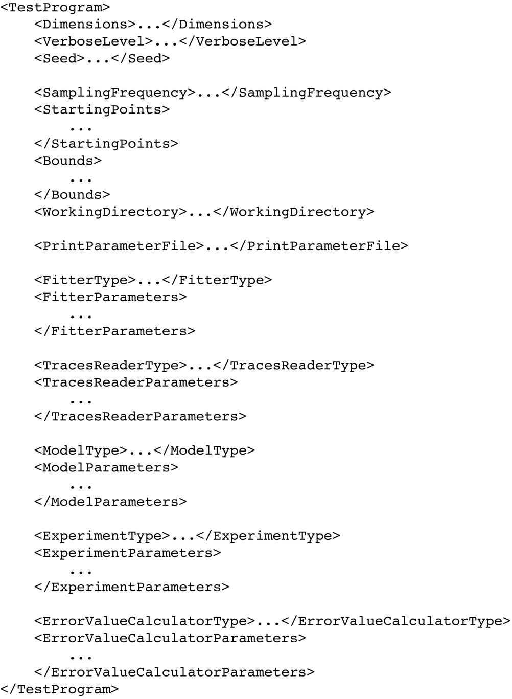
Figure 4. XML structure. The basic structure of the XML settings file. The root tag can be chosen by the user. A more extended example can be found in Appendix B.
FitterParameters contains the settings for the optimization algorithm, depending strongly on which algorithm is used, for example with evolutionary algorithm these are the size of the population, the mutation rate, etc.
ModelParameters contains the settings for the simulation software; these are fields like the location of the model, the simulation software executable, etc.
ExperimentParameters specifies the location of the files that contain the experimental data. One can, however, also use as “experimental” data the output of the model with a pre-specified set of parameters (Achard and De Schutter, 2006 ).
The ErrorValueCalculatorParameters settings control the phase-plane trajectory density method. Here one can change the size and resolution of the 2D histogram. It also specifies the location of the file containing the error values of the sets of model parameters that have already been evaluated.
The last one is the TracesReaderParameters, containing the settings for the module that reads the traces generated by the model and compares it to experimental data, and the weights that have to be given to the different parts of the traces. Here the user can also specify the stimulation protocols, the time ranges of the traces that have to be taken into account and the number of recording sites.
Parallelization
Because running complex neuron models can be computationally very expensive, and, as optimization algorithms always need to evaluate many points in the parameter space, Neurofitter supports running the software on parallel environments like computer clusters. Neurofitter is able to use the message passing interface (MPI) (Nagle, 2005 ) that is commonly in use on cluster computers.
There are different levels of parallelization (Figure 5 ) that can be used by the software. At the first level, one can let every separate node in the parallel environment calculate the entire error value of one set of parameters. This minimizes the network traffic between nodes, since the only values that have to be exchanged between the master node and the slave CPU nodes are sets of parameters and an error value. Another possibility is to split the parallelization at the level of the run parameters, this way one can run different stimulation protocols of the model on different CPU nodes. This only makes sense if one wants to run the model with a large number of different protocols, and if this number is a multiple of the number of processor nodes on the computer system. The next level that can be parallelized is outside Neurofitter's control; one can parallelize the model itself, with the PGENESIS simulator (De Schutter and Beeman, 1998 ) or with NEURON (Migliore et al., 2006 ). Neurofitter allows the user to mix the different levels of parallelization if necessary, but this can be very complicated to set up on some cluster systems as it implies starting MPI jobs from inside other MPI jobs.
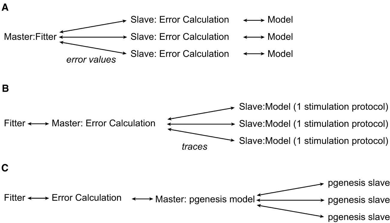
Figure 5. Parallelization. The different levels of possible parallelization. (A) All the parallel running slaves receive a set of model parameters, run the model, calculate the error value using the phase-plane trajectory density method, and return the error value to the master node. (B) The slaves run 1 stimulation protocol using the model and return the voltage traces to the master. (C) The model is internally parallelized in the neuron model simulator.
The error function
Optimization methods aim to find the minimal value of a mathematical∕computational function often called the “objective”, “fitness” or “error” function (Eiben and Smith, 2003 ). This function maps any parameter set to a real number that measures the distance between the solution and the target data. Previous research on optimization methods in the field of neurosciences has mostly used heuristic error functions (Bleeck et al., 2003 ; Bush et al., 2005 ; Davison et al., 2000 ; Druckmann et al., 2007 ; Gerken et al., 2006 ; Huys et al., 2006 ; Keren et al., 2005 ; Prinz et al., 2003 ; Reid et al., 2007 ; Schneider et al., 2004 ; Shen et al., 1999 ; Vanier and Bower, 1999 ; Weaver and Wearne, 2006 ).
We had multiple goals in selecting an error function (not to be confused with the mathematical Gauss error function “erf” (Abramowitz and Stegun, 1972 )). First of all we wanted to be able to combine smoothly experimental data from different sources like intracellular voltage recordings, local field potentials, calcium signal traces, etc., possibly recorded from different locations and during different stimulation protocols. Next, we wanted the method to be insensitive to phase shifts in spike traces (see Section Phase Shifts). Finally, the method had also to be easy to use, fast to calculate and to show little sensitivity to noise in the data. We believe that the phase-plane trajectory density method meets these conditions.
Phase-plane trajectory density method. The phase-plane trajectory density method (Bean, 2007 ; Jenerick, 1963 ; LeMasson and Maex, 2001 ) reduces the sensitivity of the error function to phase shifts between traces by eliminating the time parameter. This is achieved by plotting one time-dependent variable against another time-dependent variable; in practice usually a measure and its derivative in time. To create a phase-plane trajectory density plot from a voltage trace recording V(t), Neurofitter makes a 2D (V, dV∕dt) plot for all the data points in a specified time range (Figures 6 B and 6 D). Although specific time, and therefore phase, is removed, the density plot still constrains several temporal properties of the signal. Periodic signals like regular spiking will result in a loop with a shape dependent both on the action potential shape and on the acceleration of the depolarization during the final phase of the interspike interval. The density of data points in the loop encodes spike frequency. A burst consisting of spikes with different shapes will result in superimposed trajectories of different sizes (Figure 6 D).
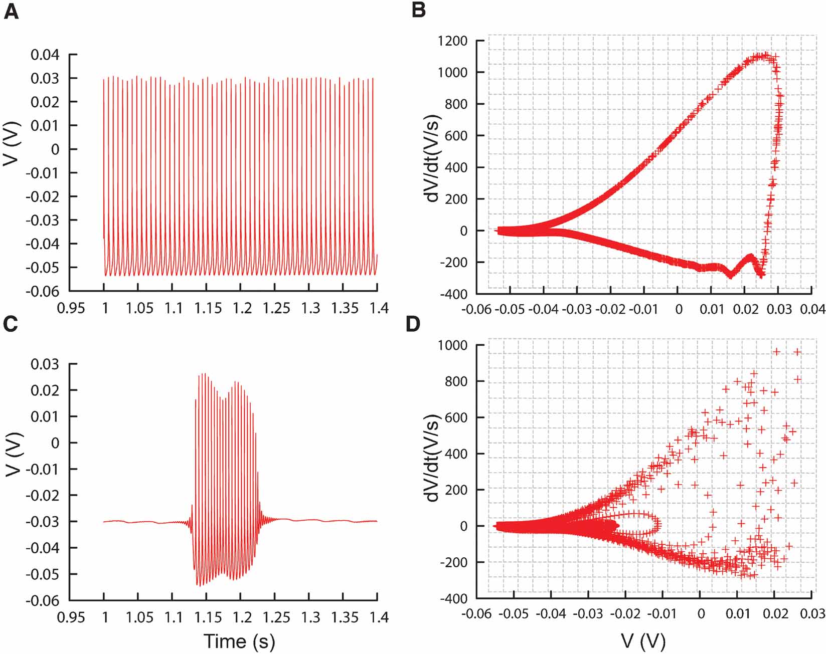
Figure 6. Phase-plane trajectory density plots. (A) Traces recorded from the PC model (De Schutter and Bower, 1994 ) during constant current injection of 0.5 nA, causing the model to tonically fire action potentials. (B) V–dV∕dt plot corresponding to the trace in (A), data sampled every 0.02 ms. Gray lines show the bins of the 2D histogram used by the phase-plane trajectory density method. In every bin the number of plot points is counted, the counts are then combined in Equation (1). (C, D) Similar to A and B, except that the model is injected with a current of 3 nA, causing it to burst. The V–dV∕dt plot shows different trajectories corresponding to different action potential shapes.
Next a two-dimensional histogram is created around the phase-plane plot. When this is done for both an experimental and a model trace, both traces can easily be compared. The error value can be computed as the root-mean-square difference between the histograms:
with dataij and modelij the number of points in bin (i, j), Ndata and Nmodel the total number of data and model points, Nx and Ny the number of bins in the histogram. A perfect match results in a zero error.
In practice, we found the optimization algorithm can have difficulties in finding an optimal value with this error definition (see Section A Bursting Pacemaker Neuron). The voltage in a neuron will remain close to the resting potential most of the time, causing the bin containing this resting value to have a large value, while the other bins representing the shape of the action potential get very small values. In Equation (1) the difference of these values to the model are then squared before taking the sum, causing the error value to become very dependent on the resting potential.
Equation (1) can be replaced by:
which has the opposite effect of the square root of the square's sum, namely that the resting potential effect loses weight. Note, however, that Equation (2) gives a proportionally higher weight to noise than Equation (1). In Neurofitter the user has to select one of these two equations.
Figure 9 compares the error landscapes obtained for a simple model using Equations (1) or (2). In this case, Equation (2) is much easier to search by an optimization algorithm as there are less local minima, so it suffices for the algorithm to follow the gradient of the surface to find a better solution.
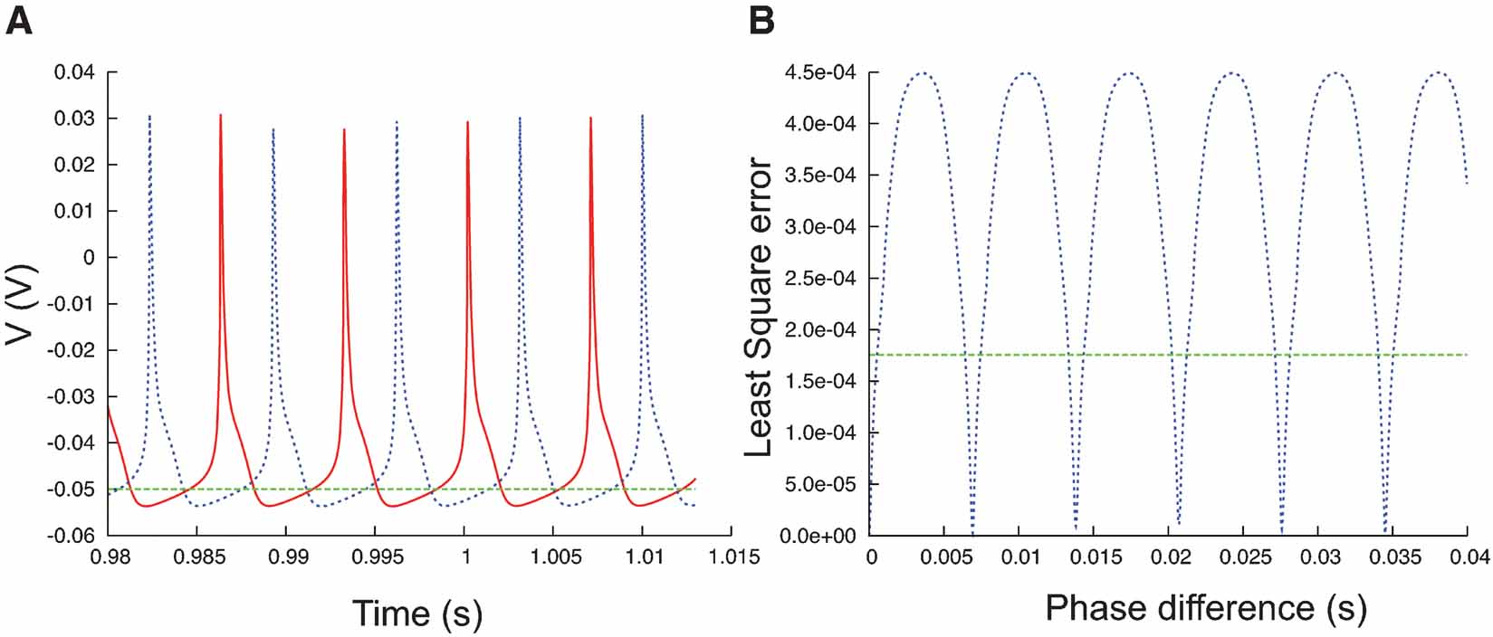
Figure 7. Phase difference between spike trains. (A) Plot of a fragment of two spike trains (red and blue) that show a phase difference. On a phase-plane trajectory density plot these two spike trains would show almost the same shape. (B) The least square errors (blue trace, Equation 3) between the two spike trains in (A) show a maximum when the phase difference is maximal, at that point the values are much higher than the least square errors between the red trace and the flat green trace (A).
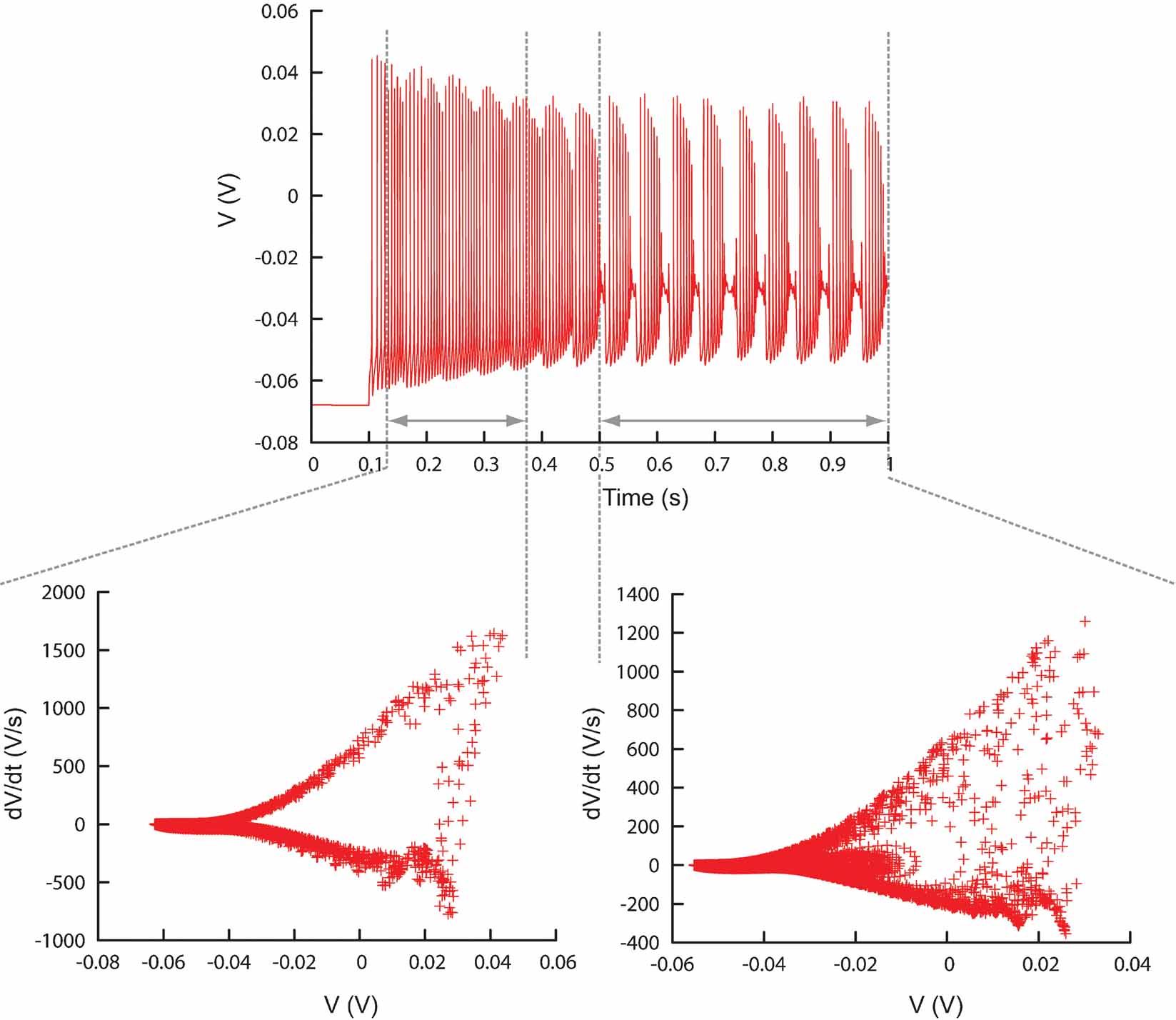
Figure 8. Different time ranges. Plot showing the ability of Neurofitter to calculate the phase-plane trajectory density plot for different time ranges in a trace separately. This enables the user to make a distinction between different firing patterns inside one trace. Example was made using the PC model (De Schutter and Bower, 1994 ).
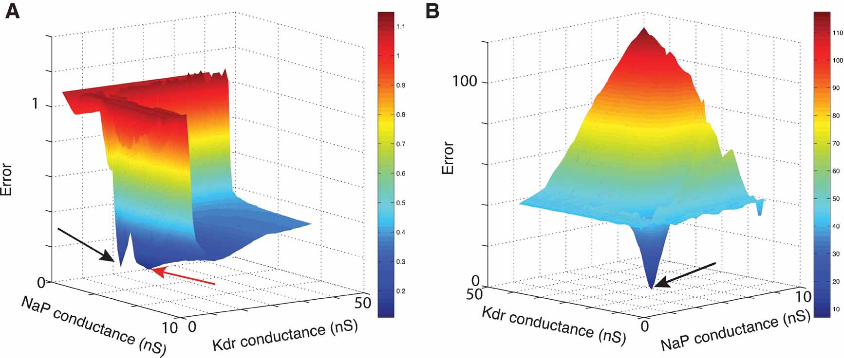
Figure 9. Error landscapes. 3D plots of error landscapes created by Mesh searches in the solution space of the pacemaker neuron model. (A) uses Equation (1) to calculate the error values; (B) uses Equation (2). Remark that the deep blue region in panel A has become dark red in panel B. The view angle of both plots is chosen differently to allow a better view of the 3D landscapes. The black arrows indicate the location of the optimal solution. The red arrow points to the position of a local minimum that created problems for the ES algorithm.
Phase shifts. For neural data it is an advantage if the error function is insensitive to small phase shifts or jitter between the model and data traces. This is very important since the exact timing of spikes is usually much less reproducible in experimental recordings than the spike shapes (Fellous et al., 2001 ; Mainen and Sejnowski, 1995 ; Shadlen and Newsome, 1998 ) and it therefore does, in general, not make sense to try to do a “perfect” fit to a particular trace.
The phase-plane trajectory density method will generate the same V-dV∕dt plot for two traces that show a small phase difference (Figure 7 A). Other techniques (Vanier and Bower, 1999 ) have compared recorded traces by calculating the mean-square error between the recorded data points:
Equation (3), however, is very sensitive to phase shifts in the data. It can even generate the undesired result that phase shifts are punished more than the difference between a spiking and a quiescent trace (Figure 7 B).
One solution would be to shift the spikes in the model trace so that both peaks coincide. This allows for comparison of the shape of the action potentials, since a lot of information about the ion channel conductances is stored in this shape. However this way of comparing traces can become complicated when one deals with traces with more than one spike: which spikes should be compared? What happens when the spiking frequencies are different? How to treat bursts with irregular number of spikes? etc.
Histogram bin size. An important setting of the method that is not automated is the size of the 2D histogram, which is determined by both the maximal∕minimal values for V and dV∕dt and by the resolution. For experimental data, it is trivial to find the extreme values for V since one possesses all the data, but for the data produced by the different model parameter sets this is in general not possible before running the models. Because of the way this matrix is implemented (see Section Implementation Aspects), these values can be chosen to be quite broad without using much extra memory to store the matrix, so one can use, for example, from −300 to 300 mV for voltage traces. If some values produced by the model fall outside these bounds the bins at the borders of the matrix are used to store overflow values. Neurofitter calculates the boundaries for dV∕dt automatically, by using the extreme values of V and the sampling rate.
The choice of the resolution (i.e., bin size) of the matrix is more difficult and is determined by a trade-off rule. If a very small bin size is chosen, the probability of finding two data points in the same bin becomes tiny, which causes two traces with a small difference to have a large error value since all their data points would be in different histogram bins. But one wants also to avoid the opposite effect, namely if the resolution is too low (in the extreme case, just 1 bin), a lot of points will be in the same bin and all traces will have very similar error values. For the problems we studied, we typically used matrix sizes in the range of 100 by 100 to 500 by 500 bins. When Neurofitter is used with a high verbose level setting, the software will print the histograms that are used on the standard output, so that the user can evaluate the size and resolution of the matrix and fine-tune them if necessary. We recommend that users check the histograms generated from the experimental data to make sure that these dimensions are set to useful values.
Combining different recordings and time ranges. Often one single experimental trace will not suffice to fit a model, and the scientist wants to combine different traces from different stimulation protocols, recording sites, etc.
To accomplish this, the error values from the different traces can be combined in a global value E as a weighted sum:
with i ranging over the Nrecordingsites different recording sites, j over the Nprotocols different stimulation protocols, and k over the Ntime ranges relevant time ranges, eijk the error values of the different traces calculated according to Equations (1) or (2) and wijk the weights of the different traces in the global error function E.
Time ranges can be specified since eliminating detailed temporal information from the data traces, as is done in the phase-plane trajectory density function, may sometimes be a disadvantage. For example, if one simulates a neuron that first spikes and then bursts, a model that produces the opposite sequence, burst first and then spike, will give good error values. This problem can be overcome by dividing the traces in different, possibly overlapping, time ranges on which the phase-plane trajectory density method is applied separately (Figure 8 , Figure 13 ).
The different error values generated this way, one for each time range, can then be summed afterwards with possibly different weights (Equation 3). These weights make it possible to assign different levels of importance to each time range. For example, it might be decided that a transitory period at the beginning of trace does not need to be fit exactly and so it can be given a lower weight. The example XML settings file in Appendix B shows how these time ranges can be defined.
Optimization algorithms
By giving an error value to every set of parameters, finding the best set of parameters is reduced to an optimization problem that can be solved by general global optimization algorithms.
Neurofitter interfaces with third-party optimizations libraries and has also several built-in optimization algorithms, ranging from very simple methods to the quite complicated particle swarm optimization. We next give a brief overview of the included algorithms.
Mesh. A multi-dimensional regular mesh is created in the parameter space (Prinz et al., 2003 ). The error function is evaluated at every vertex. No information about the goodness of points previously visited is exploited. The algorithm allows the user to make a preliminary scan of the solution space or to get insights in the shape of simple error landscapes. In the case where the model has just two parameters it is easy to make 3D plots of the error function (Figure 9 ), if there are more parameters users can apply stacking techniques to visualize higher-dimensional spaces (Taylor et al., 2006 ). As the number of points to evaluate increases as a power of the number of free parameters, this algorithm is unfortunately computationally prohibitive when this number approaches 10.
Random. This method is very similar to the Mesh algorithm, except that the points are chosen at random according to a uniform distribution in the parameter space. The advantage is that, when calculating enough points, this method does not create artificial biases in the data caused by the shape of a mesh. And since the order in which the solution space is searched is random, instead of starting at one corner, this method is more suited as a reference to compare the speed of different optimization algorithms.
File. When using the FileFitter the user provides Neurofitter with a file containing specific parameter sets that have to be evaluated. This offers the possibility of exploring some user-defined sets of parameters.
Particle swarm optimization. The particle swarm optimization algorithm (PSO) (Kennedy and Eberhart, 1995) imitates the behavior of flocks of animals that are in search for food or that try to avoid predators. The general concept is that every particle in the swarm searches for a local minimum in the error function, during which it is influenced by the best solution found so far by both the particle itself and by other particles to which it is connected to in the swarm.
Because a large number of variants for particle swarm optimization exist, James Kennedy and Maurice Clerc have proposed a standard PSO algorithm called PSO 2006 (http://www.particleswarm.info
), which is the version implemented in Neurofitter. This algorithm has a very limited amount of internal parameters that have to be set as most of these settings are calculated automatically. For example, the number of particles in the swarm is the closest integer to  with D the number of dimensions (i.e., number of parameters).
Evolution strategies (ES). Another interesting method is ES (Rechenberg, 1973 ; Schwefel, 1975 ) in which a process similar to natural selection is used to find an optimal solution. The method is very similar to genetic algorithms (Holland, 1975 ) but has as advantage that it is specifically designed for problems with real numbers instead of integers. As with genetic algorithms one starts with an initial random population of possible solutions, to which a number of operators are applied, causing subsequent populations to contain better and better individuals. The operators used in general in ES, are mutation, crossover, and selection. The former lets the parameters change with random values from a Gaussian distribution, the second averages parameters of several individuals, and the latter selects the best individuals from every generation to survive into the next.
Non-linear optimization for mixed variables and derivatives (NOMAD). NOMAD (Audet and Orban, 2004 ) is a method that, while it is still a global optimization technique, is more specialized in finding local solutions. It starts with a single point in the search space. Then the algorithm repetitively applies two steps on the search space, namely a global search and a local poll step. During the search step a mesh is created in the solution space and the value of the error function is calculated on randomly chosen crossings all over the mesh. If during this step no better solution than the incumbent solution is found, the poll step is applied. This consists of a search on the mesh in the space around the incumbent solution.
Hybrid. Unfortunately, as predicted by the no-free-lunch theorems (Wolpert and Macready, 1997 ), there exists no optimization algorithm that is perfect, and it is very difficult to find out which is the best method to use for a specific problem. However, one can combine different search algorithms by applying them sequentially (Banga et al., 2003 ). The idea is to first let one algorithm search in the full parameter space until it is unable to substantially improve the solution, and then use its best solution as a start for another algorithm that is faster at finding local solutions. In Neurofitter we have implemented a method that first uses the ES technique, which is then followed by the NOMAD algorithm (Achard and De Schutter, submitted).
Implementation aspects
Neurofitter is written in C++ in such a way that is very readable by users who have some knowledge of C++. Overall, concepts in Neurofitter are used in a very generic way, so that users can easily add pieces of code to Neurofitter. In this way other optimization algorithms, file formats, parallelization methods, etc. can be incorporated into Neurofitter. The settings of all the components that are added can be read from the Neurofitter XML settings file in a straightforward way.
We have minimized the memory used by Neurofitter by implementing the V-dV∕dt histograms in a data structure called a dictionary. Since these histograms are in general very sparse, it is not very memory efficient to store all the values in memory arrays, but only to store the non-zero elements, which can be implemented using a two-dimensional dictionary. As a consequence, users can set the minimal and maximal values of the matrix quite broadly without incurring a memory penalty.
We realize that the field of optimization techniques is a rapidly evolving field and that many new optimization methods are being developed. That is why we made it possible for users to use third-party optimization libraries. Similarly, users are free to use whichever neuron simulator they like. We provided built-in interfaces to the NEURON (Hines and Carnevale, 1997 ) and GENESIS (Bower and Beeman, 1998 ) simulators but other simulators can easily be used.
Since we expect a very diverse set of users, Neurofitter compiles on as many systems as possible. Some of the systems we successfully tested Neurofitter on include Mac OS × 10.4 on PPC∕Intel processors, Windows Cygwin, Linux Slackware∕Suse, etc. Neurofitter uses MPI for it's parallelized version and can be used on most cluster computers, the MPI implementation we tested it on were OpenMPI, LAM∕MPI and MPICH.
Methods used in the examples
The two example models in the discussion section were simulated with GENESIS 2.2.1 software (Bower and Beeman, 1998 ) under Mac OS X 10.4 and SUSE Linux Enterprise Server 10 and run on an Apple cluster computer using IBM PowerPC G5 and Intel Xeon processors. For the compilation of Neurofitter, GENESIS, ES, and NOMAD the Gnu Compiler Collection (gcc) version 4.0.1 was used. Data analysis was performed using Matlab 6.5, Igor Pro 5.04b and Gnuplot 4.2.
Examples of Using Neurofitter
A bursting pacemaker neuron
Rhythm generation is an important function of the nervous system. The primary kernel for respiratory rhythm is hypothesized to be located in the pre-Bötzinger complex in mammals (Smith et al., 1991 ). The rhythm is generated by a population of excitatory neurons that have intrinsic bursting pacemaker-like properties. These properties arise from a balance between the different ion channels present in the cells. We tested the efficiency of Neurofitter in finding the correct balance of the parameters that generate this bursting behavior by letting it fit a simple single-compartmental model of the pre-Bötzinger bursting pacemaker neurons described in (Butera et al., 1999 ). It contains four ionic currents: a fast (NaF) and a persistent (NaP) Na current, a delayed-rectifier potassium (Kdr) current, and a K-dominated passive leakage current:

To allow for a bursting behavior the model incorporates a slow inactivation of the NaP current with a time constant of 10 seconds.
This model was a good test case as it has a small number of ionic channels but an electrophysiological behavior more complex than simple spiking. Two of the four maximal conductances were released, creating an error function that takes two single values as argument and that could easily be visualized in a three-dimensional plot (Figure 9 A). We fitted the maximal conductances of the NaP and Kdr channels, since the balance of strengths of these two channels is important to allow the bursting behavior of the model.
The target traces were these created by the original maximal conductances values used in (Butera et al., 1999
), 2.8 nS for  and 11.2 nS for
  . The parameter boundaries imposed on the optimization algorithms were [0,10] nS for and [0,50] nS for . We used a single phase-plane 2D histogram comprising 3.0–4.8 second of the trace shown in Figure 11
A.
. The parameter boundaries imposed on the optimization algorithms were [0,10] nS for and [0,50] nS for . We used a single phase-plane 2D histogram comprising 3.0–4.8 second of the trace shown in Figure 11
A.
A mesh in the solution space was explored, by using Equation (1) to calculate the difference between two matrices, creating the error plot shown in Figure 9 A.
However, optimization algorithms often failed to find a good solution to this error function. This was because the error function contained a local minimum around the point and  , while the best solution was 2.8 nS for and 11.2 nS for (Figure 10
).
, while the best solution was 2.8 nS for and 11.2 nS for (Figure 10
).
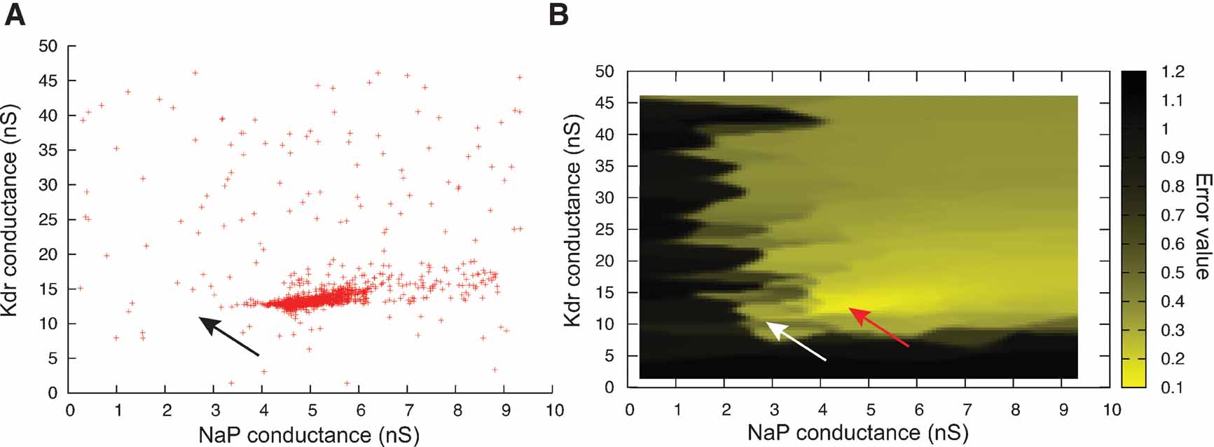
Figure 10. ES search using Equation (1) in the phase-plane trajectory density method. (A) Plot of points in the solution space evaluated by Neurofitter during an Evolutionary Strategies search (6000 evaluations) to tune the pacemaker model using Equation (1) for the phase-plane trajectory density method. Every red point represents 1 evaluation. ES is not able to escape a deep region (B) Interpolated plot of the error values calculated by Neurofitter during the ES search in (A). The global optimal solution with error value 0 is shown by the black and white arrows, but the ES algorithm is not able to escape a local minimum (red arrow) around  and
and  . Remark that plot B does not show a complete representation of the error landscape, but only the shape as seen by ES.
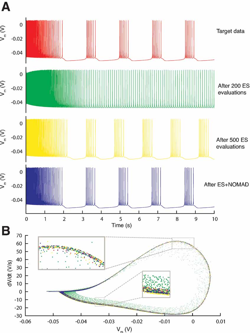
Figure 11. Resulting traces. (A) Somatic membrane voltage traces of the target data (red), the best model found by an ES optimization after 200 (green) and 500 (yellow) evaluations, and by a NOMAD search that started with the best solution found by ES (blue). The respective error values are 0, 6.7, 4.1, and 2.6. (B) Phase-plane trajectory of the traces in A (same color code). The density of the trajectory is not visible, since one location on the plot can contain many overlapping data points.
Further investigation revealed that this was because the error function using Equation (1), emphasized too much the resting potential, and less the shape of the action potentials, as described in Section Phase-Plane Trajectory Density Method.
Using Equation (2) the error landscape became steeper and contained less local optima (Figure 9 B), which made it easier for an optimization algorithm to find a good solution. Running ES and NOMAD sequentially made it possible in this case to find almost the exact value that was used in the original paper by making 1000 model evaluations (Figure 11 ).
To benchmark the optimization algorithms, we made a comparison with a complete random search of the solution space (Figure 12 ), which shows that, indeed, the more advanced optimization algorithms were faster in finding a good solution.
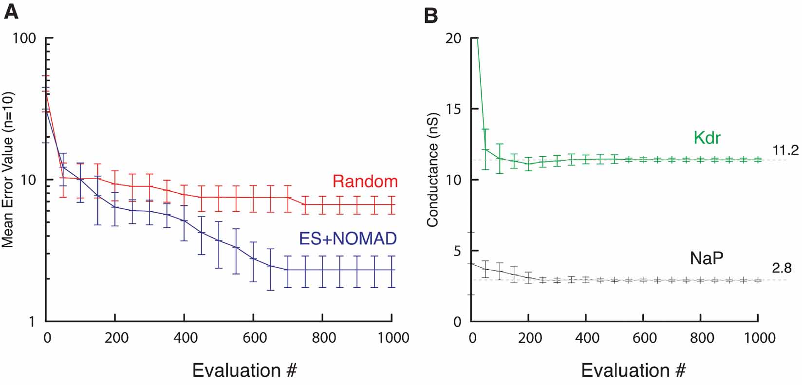
Figure 12. ES∕NOMAD evolution of pacemaker neuron model. (A) Evolution of best error value found by Random (red) and hybrid ES+NOMAD (blue) searches. The data points (mean ± sdv) are averaged over 10 different runs of the algorithms using different random seeds. After 500 error evaluations Neurofitter switched from ES to NOMAD. (B) The evolution of the best maximal NaP and Kdr channel conductances during the same 10 runs as in A for the hybrid ES + NOMAD algorithm. The dashed line shows the maximal conductance of the target data. Not the entire range of the y-axis is shown to allow a better scaling of the plot.
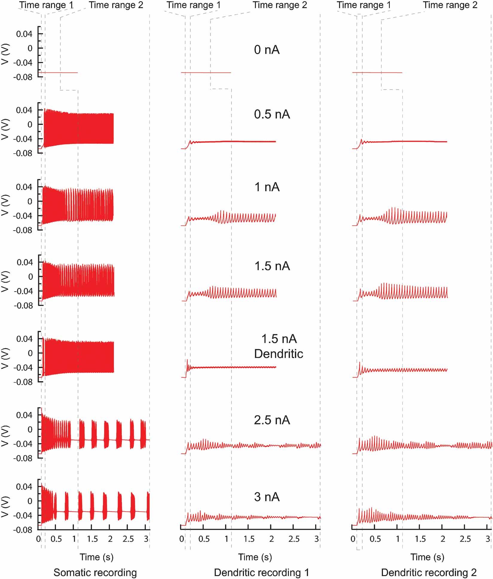
Figure 13. PC model traces. All the traces recorded from the original PC model that were used to find new parameters. Every column represents a different recording site, every row a different current injection (somatic injection unless otherwise mentioned) and the dashed lines show the boundaries of the two different time ranges. In total there are 42 trace fragments for which separate phase-plane trajectory plots are calculated. The traces with no current injection have a slightly different time range. For the other current injection amplitudes the time range ends at the end of the recording.
The XML settings file used for this example can be found in Appendix B.
A complex multi-compartmental neuron
The Purkinje cell (PC) model described in (De Schutter and Bower, 1994 ) is a very complex model consisting of 1600 compartments and 4 zones with different channel densities. The model shows a very broad range of possible activities (tonic firing, bursting, etc). Therefore, it has a large amount of parameters that have to be fit before it can reproduce the available experimental data. This makes it very difficult to hand-tune this model and it is quite appropriate to use automatic optimization techniques. Results of this approach have been described in (Achard and De Schutter, 2006 ). A total of 24 of maximal conductance parameters were released (Table 1 ), and current clamp experiments using different injection amplitudes were simulated. While we tried to use reasonably wide bounds for all conductances in these parameter searches (Table 1 ), preliminary tests showed that the bounds for the two channels controlling somatic spiking (fast sodium and delayed rectifier potassium) had to be quite constrained for the ES to work rapidly in this example.
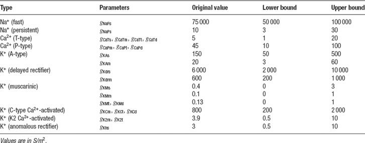
Table 1. The 24 maximal conductance parameters of the PC model that were tuned in Neurofitter.
This study made extensive use of the ability of Neurofitter to split up data traces and to combine different phase-plane plots to generate one error function. To incorporate different behaviors of the PC, currents of different amplitudes were injected in both soma and dendrites (Figure 13 ). Traces were obtained during five somatic current injections of 0.5, 1, 1.5, 2.5, and 3 nA; one dendritic current injection of 1.5 nA; and without any injected current to include the quiescence at rest (De Schutter and Bower, 1994 ). The model was run sequentially for different current amplitudes, creating seven different output files. The duration of recording was different for the each injected current: it was short for the silent or tonically firing traces in order to optimize the computation time and longer for bursting traces in order to have enough points in the error 2D histogram.
Since ion channel parameters were fitted in the soma and the dendrites it was important to have recording sites in both locations (Figure 13 ). These were weighted so that soma and dendrite had equal influence on the error measure. In order to have an experimentally realistic protocol, the dendritic recording sites were only located on smooth dendrites. Every recorded file from the model therefore contained four columns, one column with the timestamps, one column with data recorded from the soma and two from the dendrites.
After the start of a current injection one can expect a transitory regime that stabilizes after some time. To separate these two periods, every trace was evaluated twice using the time range feature of Neurofitter (Figure 13 , Section Combining Different Recordings and Time Ranges). The transitory period was defined as the period from 100 to 200 ms after the start of the experiment and the stable period as from 1 second after the start of current injection until the end of the recording.
The combination of all these recordings created 7 × 3 × 2 parts of traces that were compared separately using the phase-plane trajectory density method with Equation (1) and Nx = Ny = 100.
Combining all the measures with different weights wijk a total error value could be calculated:
with i iterating over the injection amplitudes, j over the recording sites, and k over the time ranges; wijk 1 for somatic recordings and 0.5 for dendritic recordings, except when no current was injected, then they were respectively 0.6 and 0.3.
As optimization algorithm the ES technique was used to fit the parameters, the evolution of the error values during the algorithm is shown in Figure 14 .
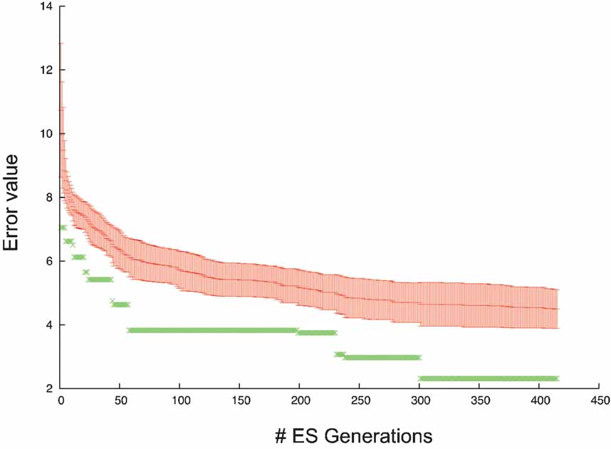
Figure 14. Error evolution PC model. Error evolution during the optimization process of the PC model. Mean error value ± standard deviation in every generation is in red. The error value of the best individual is in green.
Subsequent analysis showed that a hybrid approach (Section Hybrid) substantially improved the error of the solutions found compared to ES alone (Achard and De Schutter, submitted).
Discussion
As the results show, Neurofitter finds model parameter sets that nicely reproduce predefined target voltage traces, with minimal effort from the user. For a very simple model (Butera et al., 1999 ) with only two released parameters, Neurofitter finds one almost perfect solution, but for a more complicated model of the cerebellar PC (De Schutter and Bower, 1994 ) the method has shown that the different sets of parameters can generate data traces that show very similar behavior (Achard and De Schutter, 2006 ). These two examples were chosen because we knew in advance that a good solution exists and, therefore, any problems in fitting would be due to the error measure or optimization method used. Of course Neurofitter also needs to be shown capable of fitting models to real experimental data, but this is more complex to analyze as the quality of the neuron model used will determine the ultimate success. Preliminary efforts in fitting experimental traces (http://icwww.epfl.ch/~gerstner/QuantNeuronMod2007/challenge.html ) have been very encouraging and this is a topic of active research by the authors.
One of the big advantages of Neurofitter lies in its use of the phase-plane trajectory density method. In our experience it is a very efficient method to evaluate time series data traces and it has the desirable property of being insensitive to jitter and phase shifts in the data (Druckmann et al., 2007 ). This error measure is entirely heuristic and it is difficult to predict a priori a reasonable threshold to distinguish good from bad models (Achard and De Schutter, 2006 ). The use of Equation (2), which introduces a very sharp gradient for small errors and a low gradient for large errors, is also unusual but it worked quite well for different fitting problems we have investigated. A limitation of the phase-plane trajectory density method is that it only provides information about size of error if the model and data traces overlap. If there is no such overlap the maximal error will be computed, independent of the distance between the traces in 2D space. However, this is unlikely to occur if the error measure combines several phase-planes (Equation 5), and it will never cause problems if enough parameter sets are randomly generated at early stages of the optimization.
Previously described automated model parameter search methods differ from Neurofitter on two separate aspects: the optimization method used and the implementation of the error function. Some methods (Goldman et al., 2001 ; Prinz et al., 2003 ) use an error function that focuses on quantitative aspects that are important for physiological function and are therefore also insensitive to phase shifts in the data. Typical properties include the firing behavior (silent, spiking, bursting,…), resting potentials, spiking frequencies, spike heights, spike widths, bursting frequencies, number of spikes per burst, etc. These properties are measured from the data and compared to similar measurements from the model to calculate the error. We have previously shown that our method achieves the same accuracy as these approaches (Achard and De Schutter, 2006 , Supplementary data). This approach requires criteria to consistently define spikes, bursts, “regularly spiking”, etc. It necessitates the use of spike detection or even spike sorting methods (Lewicki, 1998 ) to analyze the traces, and, as these methods are at best semi-automated, extra effort from the user will be required. An advantage of these approaches is that the model will not be fitted to data from a single cell but to a statistical distribution reflecting the underlying variability (Marder and Goaillard, 2006 ). It also makes it easier to give more weight to specific characteristics, like spike width (Druckmann et al., 2007 ). But even in intracellular recordings the reliability of automated spike isolation methods is not always guaranteed (Blanche and Swindale, 2006 ; Moon, 1996 ; Paulin, 1992 ). If one wants to reproduce not only the simple spiking activity of a cell or a network, but also its subthreshold behavior, the spikelets of the bursts, the transmission of post-synaptic potentials, etc., it becomes increasingly difficult to automatically quantify these different properties. Moreover, the more complex the analysis required, the more subjective and user-dependent it will become since the criteria that have to be used are not clearly defined. Conversely, the phase-plane trajectory density method used by Neurofitter is very transparent and requires only a few control parameters, allowing the user to focus on the selection of relevant data traces to determine the seminal properties of the model. While we have until now only included data from one cell or neuron in the error measure it is, in principle, possible to combine data from different neurons of a similar type if one wants to generate a “generic” model.
Another advantage of using Neurofitter is that the user can exploit the large knowledgebase that exists in the field of optimization techniques. Very advanced methods have been invented in this field, and by using Neurofitter one can apply many of these techniques to tune neuronal models, including evolutionary strategies (Keijzer et al., 2001 ), particle swarm optimization (Kennedy and Eberhart, 1995 ) and MADS (Audet and Orban, 2004 ). Especially the ES technique has been shown to be able to handle high dimensional problems with a lot of local minima (Achard and De Schutter, 2006 ; Banga et al., 2003 ). Global optimization techniques, that try to find the best global minimum of the error function will perform better than local optimization techniques, since the error space created by the parameter of neuron models is apparently filled with local minima and flat area's (Achard and De Schutter, 2006 ; Goldman et al., 2001 ). So methods that are based on optimization algorithms like the conjugate gradient method (Vanier and Bower, 1999 ) will have difficulties in finding good solutions.
Other parameter search methods (Bhalla and Bower, 1993 ; Goldman et al., 2001 ; Prinz et al., 2003 ) explore the solution space using brute-force methods by evaluating the model on all the points of a uniform higher-dimensional mesh. This is reasonable when the number of parameters that need to be fitted remains low, but since the amount of points that needs to be evaluated increases as a power of the number of dimensions, this becomes computationally very expensive for complex models.
The method proposed by Huys et al. (2006) is an interesting alternative, because it does not apply the traditional stochastic search methods to tune neuron models, but follows a more direct mathematical approach by turning the fitting problem into a non-negative regression problem. However, its main disadvantage is that for large cells it requires voltage recording at many positions in the neuron, which strongly limits the data sets that can be used for this method since at present the only technique available would be voltage-sensitive dye imaging studies.
In this paper, the use of current clamp voltage data is emphasized, but this is in no sense a prerequisite to use Neurofitter. Users can easily use it for other applications. As long as the experimental data consists of one or more time-dependent traces to which the phase-plane matrix method can be applied, Neurofitter can be used. Possible alternatives are traces of calcium concentration signals inside a cell, data from voltage clamp experiments, etc. It has recently been suggested that extracellular recordings of action potentials can provide useful additional constraints to fitting a model (Gold et al., 2006 ) and it is relatively straightforward to incorporate such data into phase-plane trajectory density matrices. It should also be possible to apply Neurofitter to other problems than fitting the maximum conductances of channels. For example, instead of using a fixed morphology, one may want to tune the morphology itself to generate particular electrophysiological properties (Mainen and Sejnowski, 1996 ; Stiefel and Sejnowski, 2007 ). Another possibility is fitting of network parameters, including connection strengths between neurons, network topologies, etc. This will require careful evaluation of the required experimental data, especially if one wants to achieve specified levels of synchronization in the network (Brown et al., 2004 ).
Neurofitter will hopefully stimulate both modelers and experimentalists to share their data to create better models (Ascoli, 2006 ; Kennedy, 2006 ), and will make it easier for neuroscientists to create detailed neuron models based on experimental data. Neurofitter is designed to be an evolving software package. We are continuing to explore ways to enhance it, both by improving the search methods used and by making the program easier to use. As Neurofitter is licensed under GPL license, it can be modified and extended by its users.
Downloading the software
Neurofitter can be freely downloaded from http://neurofitter.sourceforge.net .
Conflict of Interest Statement
The authors declare that the research was conducted in the absence of any commercial or financial relationships that could be construed as a potential conflict of interest.
Acknowledgements
W. V. G. is funded as an FWO research assistant. This work was supported by grants from BOF (UA), FWO Flanders and HFSPO and OIST.
Appendix A: Algorithm
Using Neurofitter involves the following steps:
(1) The user adapts the model so that it can interact with Neurofitter
(2) The user adapts the experimental data to the appropriate format
(3) The user generates an XML file containing the settings of Neurofitter
(4) The user executes the Neurofitter binary
(5) Neurofitter reads the experimental data and generates the experimental phase-plane trajectory density matrices
(6) Neurofitter starts the optimization algorithm
(7) The optimization algorithm returns a first set of model parameters that have to be evaluated
(8) For every “run” parameter (e.g., amplitude of injected current)
8.1 Neurofitter writes a file “param.dat” in the model directory containing the model parameters
8.2 Neurofitter writes the “run” parameter (e.g., current amplitude) in ‘param.dat’
8.3 Neurofitter writes in ‘param.dat’ a string containing the location of where it expects the simulator to write the output data
8.4 Neurofitter runs the external neuron simulator
8.5 The simulator reads the model parameters from ‘param.dat’
8.6 The simulator reads the run parameter from ‘param.dat’
8.7 The simulator reads the requested output file location from ‘param.dat’
8.8 The simulator runs the model
8.9 The simulator writes out the data to the requested location
8.10 Neurofitter reads the output of the simulator
8.11 Neurofitter cuts out the relevant time periods in the data and generates phase-plane trajectory density matrices
8.12 Neurofitter calculates the error value for this run by comparing with the experimental V phase-plane trajectory density matrices
(9) Neurofitter calculates the weighted sum of the error values of all the different runs
(10) Neurofitter writes the error value of the parameters in the Neurofitter output file
(11) Neurofitter gives back the error value of the model parameter set to the optimization algorithm
(12) The optimization algorithm searches for a new parameter set to evaluate
(13) Neurofitter returns to step (8) until a termination criterion is reached
(14) The user reads all the evaluated model parameter sets with their error value from the Neurofitter output file.
Appendix B: File Formats Used By Neurofitter
Data traces file format
The first column of every file contains the time stamps, and in subsequent columns the data recorded from the different recording sites (Figure 3 ). The sampling rate of all the files should be the same.
The data (both the experimental data and the model output) has to be stored using filenames that have as format “output_Run0.dat”, “output_Run1.dat”, etc. The user can choose the text string before the underscore by setting the value of the OutputFilePrefix option in the Neurofitter XML settings file (section below). The format of the text after the underscore is fixed; it should be “Run0.dat”, “Run1.dat”, “Run2.dat”, etc. for the files containing the data that will be compared with stimulation protocols 0, 1, 2, etc.
XML settings file
An example of a Neurofitter settings file. It is similar to the one used for the model in Section A Bursting Pacemaker Neuron, but for demonstration purposes some settings in this file are different. All words between <!- and -> are comments, and are not processed by Neurofitter.
References
Abramowitz, M., and Stegun, I. A. (1972). Handbook of mathematical functions with formulas, graphs, and mathematical tables. (New York, Dover).
Achard, P., and De Schutter, E. (2006). Complex parameter landscape for a complex neuron model. PLoS Comput. Biol. 2, e94.
Audet, C., and Orban, D. (2004). Finding optimal algorithmic parameters using a mesh adaptive direct search. Cahiers du GERAD G-2004-xx.
Baldi, P., Vanier, M. C., and Bower, J. M. (1998). On the use of Bayesian methods for evaluating compartmental neural models. J. Comput. Neurosci. 5, 285–314.
Banga, J. R., Moles, C. G., and Alonso, A. A. (2003). Global optimization of bioprocesses using stochastic and hybrid methods. In Frontiers in Global Optimization (Nonconvex Optimization and Its Applications), C. A. Floudas, and P. M. Pardalos, eds. (Kluwer Academic Publishers).
Bean, B. P. (2007). The action potential in mammalian central neurons. Nat. Rev. Neurosci. 8, 451–465.
Bhalla, U. S., and Bower, J. M. (1993). Exploring parameter space in detailed single neuron models: simulations of the mitral and granule cells of the olfactory bulb. J. Neurophysiol. 69, 1948–1965.
Bjaalie, J. G., and Grillner, S. (2007). Global neuroinformatics: the international neuroinformatics coordinating facility. J. Neurosci. 27, 3613–3615.
Blanche, T. J., and Swindale, N. V. (2006). Nyquist interpolation improves neuron yield in multiunit recordings. J. Neurosci. Methods 155, 81–91.
Bleeck, S., Patterson, R. D., and Winter, I. M. (2003). Using genetic algorithms to find the most effective stimulus for sensory neurons. J. Neurosci. Methods 125, 73–82.
Bower, J. M., and Beeman, D. (1998). The book of GENESIS: Exploring realistic neural models with the GEneral NEural SImulation System, 2nd ed. (New York, Springer-Verlag).
Brown, E. N., Kass, R. E., and Mitra, P. P. (2004). Multiple neural spike train data analysis: state-of-the-art and future challenges. Nat. Neurosci. 7, 456–461.
Bush, K., Knight, J., and Anderson, C. (2005). Optimizing conductance parameters of cortical neural models via electrotonic partitions. Neural Netw. 18, 488–496.
Butera, R. J., Rinzel, J., and Smith, J. C. (1999). Models of respiratory rhythm generation in the pre-Bötzinger complex. I. Bursting pacemaker neurons. J. Neurophysiol. 82, 382–397.
Davison, A. P., Feng, J., and Brown, D. (2000). A reduced compartmental model of the mitral cell for use in network models of the olfactory bulb. Brain Res. Bull. 51, 393–399.
De Schutter, E., and Beeman, D. (1998). Speeding up GENESIS simulations. In The Book of GENESIS Exploring Realistic Neural Models with the GEneral NEural SImulation System. (Berlin, Springer).
De Schutter, E., and Bower, J. M. (1994). An active membrane model of the cerebellar Purkinje cell. I. Simulation of current clamps in slice. J. Neurophysiol. 71, 375–400.
De Schutter, E., and Steuber, V. (2000). Modeling of neurons with active dendrites. In Computational Neuroscience: Realistic Modeling for Experimentalists, E. De Schutter, eds. (Boca Raton, CRC Press).
De Schutter, E., Ekeberg, O., Kotaleski, J. H., Achard, P., and Lansner, A. (2005). Biophysically detailed modelling of microcircuits and beyond. Trends Neurosci. 28, 562–569.
Druckmann, S., Banitt, Y., Gidon, A., Schuermann, F., Markram, H., and Segev, I. (2007). A novel multiple objective optimization framework for constraining conductance-based neuron models by experimental data. Front. Neurosci. 1.
Fellous, J. M., Houweling, A. R., Modi, R. H., Rao, R. P., Tiesinga, P. H., and Sejnowski, T. J. (2001). Frequency dependence of spike timing reliability in cortical pyramidal cells and interneurons. J. Neurophysiol. 85, 1782–1787.
Forrest, S., and Mitchell, M. (1993). What makes a problem hard for a genetic algorithm? Some anomalous results and their explanation. Mach. Learn. 13, 285–319.
Foster, W. R., Ungar, L. H., and Schwaber, J. S. (1993). Significance of conductances in Hodgkin-Huxley models. J. Neurophysiol. 70, 2502–2518.
Gerken, W. C., Purvis, L. K., and Butera, R. J. (2006). Genetic algorithm for optimization and specification of a neuron model. Neurocomputing 69, 1039–1042.
Gold, C., Henze, D. A., Koch, C., Buzsáki, G. (2006). On the origin of the extracellular action potential waveform: A modeling study. J. Neurophysiol. 95, 3113–3128.
Goldman, M. S., Golowasch, J., Marder, E., and Abbott, L. F. (2001). Global structure, robustness, and modulation of neuronal models. J. Neurosci. 21, 5229–5238.
Golowasch, J., Goldman, M. S., Abbott, L. F., and Marder, E. (2002). Failure of averaging in the construction of a conductance-based neuron model. J. Neurophysiol. 87, 1129–1131.
Hines, M. L., and Carnevale, N. T. (1997). The NEURON simulation environment. Neural Comput. 9, 1179–1209.
Hines, M. L., Morse, T., Migliore, M., Carnevale, N. T., and Shepherd, G. M. (2004). ModelDB: A database to support computational neuroscience. J. Comput. Neurosci. 17, 7–11.
Holland, J. H. (1975). Adaptation in natural and artificial systems: an introductory analysis with applications to biology, control, and artificial intelligence (Ann Arbor, University of Michigan Press).
Huys, Q. J., Ahrens, M. B., and Paninski, L. (2006). Efficient estimation of detailed single-neuron models. J. Neurophysiol. 96, 872–890.
Jenerick, H. (1963). Phase plane trajectories of the muscle spike potential. Biophys. J. 3, 363–377.
Keijzer, M., Merelo, J. J., Romero, G., and Schoenauer, M. (2001). Evolving objects: A general purpose evolutionary computation library. In Artificial Evolution: 5th International Conference, Evolution Artificielle, EA 2001, Le Creusot. (France; Berlin, Springer-Verlag).
Kennedy, D. (2006). Where's the beef? missing data in the information age. Neuroinformatics 4, 271–273.
Kennedy, J., and Eberhart, R. C. (1995). Particle swarm optimization. Proceedings of the IEEE International Joint Conference on Neural Networks, 1942-1948.
Keren, N., Peled, N., and Korngreen, A. (2005). Constraining compartmental models using multiple voltage recordings and genetic algorithms. J. Neurophysiol. 94, 3730–3742.
LeMasson, and Maex (2001). Introduction to equation solving and parameter fitting. In Computational Neuroscience: Realistic Modeling for Experimentalists. (London, CRC Press).
Lewicki, M. S. (1998). A review of methods for spike sorting: the detection and classification of neural action potentials. Network 9, R53–R78.
Mainen, Z. F., and Sejnowski, T. J. (1995). Reliability of spike timing in neocortical neurons. Science 268, 1503–1506.
Mainen, Z. F., and Sejnowski, T. J. (1996). Influence of dendritic structure on firing pattern in model neocortical neurons. Nature 382, 363–366.
Marder, E., and Goaillard, J. M. (2006). Variability, compensation and homeostasis in neuron and network function. Nat. Rev. Neurosci. 7, 563–574.
Migliore, M., Cannia, C., Lytton, W. W., Markram, H., and Hines, M. L. (2006). Parallel network simulations with NEURON. J. Comput. Neurosci. 21, 119–129.
Moon, B. R. (1996). Sampling rates, aliasing, and the analysis of electrophysiological signals. Biomedical Engineering Conference, 1996, Proceedings of the 1996 Fifteenth Southern Biomedical Engineering Conference, 1996., Proceedings of the 1996 Fifteenth Southern Sampling rates, aliasing, and the analysis of electrophysiological signals, 401–404.
Nagle, D. (2005). MPI – The Complete Reference, Vol. 1: The MPI Core, 2nd ed., Scientific and Engineering Computation Series by Marc Snir, Steve Otto, Steven Huss-Lederman, David Walker, and Jack Dongarra. Sci. Program. 13, 57–63.
Prinz, A. A., Billimoria, C. P., and Marder, E. (2003). Alternative to hand-tuning conductance-based models: construction and analysis of databases of model neurons. J. Neurophysiol. 90, 3998–4015.
Rall, W. (1964). Theoretical significance of dendritic trees for neuronal input–output relations. In Neural Theory and Modeling, R. F. Reiss, eds. (Stanford, California, Stanford University Press).
Rall, W., Burke, R. E., Holmes, W. R., Jack, J. J., Redman, S. J., and Segev, I. (1992). Matching dendritic neuron models to experimental data. Physiol. Rev. 72, S159–S186.
Rechenberg, I. (1973). Evolutionsstrategie: optimierung technischer systeme nach prinzipien der biologischen evolution. (Stuttgart, Germany, Frommann-Holzboog).
Reid, M. S., Brown, E. A., and De Weerth, S. P. (2007). A parameter-space search algorithm tested on a Hodgkin-Huxley model. Biol. Cybern. 96, 625–634.
Schneider, S., Igel, C., Klaes, C., Dinse, H. R., and Wiemer, J. C. (2004). Evolutionary adaptation of nonlinear dynamical systems in computational neuroscience. Genet. Programming Evolvable Mach. 5, 215–227.
Shadlen, M. N., and Newsome, W. T. (1998). The variable discharge of cortical neurons: implications for connectivity, computation, and information coding. J. Neurosci. 18, 3870–3896.
Shen, G. Y., Chen, W. R., Midtgaard, J., Shepherd, G. M., and Hines, M. L. (1999). Computational analysis of action potential initiation in mitral cell soma and dendrites based on dual patch recordings. J. Neurophysiol. 82, 3006–3020.
Smith, J. C., Ellenberger, H. H., Ballanyi, K., Richter, D. W., and Feldman, J. L. (1991). Pre-Bötzinger complex: a brainstem region that may generate respiratory rhythm in mammals. Science 254, 726–729.
Stiefel, K. M., and Sejnowski, T. J. (2007). Mapping function onto neuronal morphology. J. Neurophysiol. 98, 513–526.
Taylor, A. L., Hickey, T. J., Prinz, A. A., and Marder, E. (2006). Structure and visualization of high-dimensional conductance spaces. J. Neurophysiol. 96, 891–905.
Traub, R. D., Wong, R. K., Miles, R., and Michelson, H. (1991). A model of a CA3 hippocampal pyramidal neuron incorporating voltage-clamp data on intrinsic conductances. J. Neurophysiol. 66, 635–650.
Vanier, M. C., and Bower, J. M. (1999). A comparative survey of automated parameter-search methods for compartmental neural models. J. Comput. Neurosci. 7, 149–171.
Keywords: parameter tuning, neuron, model, simulator, automatic, optimization algorithms, software, electrophysiology
Citation: Werner Van Geit, Pablo Achard and Erik De Schutter (2007). Neurofitter: A parameter tuning package for a wide range of electrophysiological neuron models. Front. neuroinform. 1:1. doi: 10.3389/neuro.11/001.2007
Received: 30 August 2007;
Paper pending published: 10 September 2007;
Accepted: 24 September 2007;
Published online: 2 November 2007
Associate Editor:
Jan G. Bjaalie, International Neuroinformatics Coordination Facility, Stockholm, Sweden; University of Oslo, Oslo, NorwayReview Editors:
Robert C. Cannon, Textensor Limited, Edinburgh, United KingdomMichael Hines, Yale University, New Haven, USA
Copyright: © 2007 Van Geit, Achard, De Schutter. This is an open-access article subject to an exclusive license agreement between the authors and the Frontiers Research Foundation, which permits unrestricted use, distribution, and reproduction in any medium, provided the original authors and source are credited.
*Correspondence: Erik De Schutter, Computational Neuroscience Unit, Okinawa Institute of Science and Technology, 7542 Onna, Onna-son, Kunigami, Okinawa 904-0411, Japan. e-mail: erik@oist.jp