Imbalanced classification applied to asteroid resonant dynamics

1 Introduction

Studying resonant dynamics in the asteroid belt using machine learning (ML) is a relatively new field of research. One of our initial works in this area applied a perceptron neural network to classify resonant arguments of asteroids affected by the exterior M1:2 mean-motion resonance with Mars Carruba et al. (2021a). Genetic algorithms were then used to optimize ML methods to study the population of asteroids interacting with the z₁ and z₂ non-linear secular resonances Carruba et al. (2021b). More recently, perceptron Carruba et al. (2022b) and advanced convolutional neural network models, like the VGG, Inception, and ResNet Carruba et al. (2022a), have been used to study the population of asteroids interacting with the ν₆ secular resonance.

However, one problem with these databases is that, in some cases, we observe a severe imbalance between the number of asteroids identified as resonant, and the remaining, more numerous population. The imbalance can be slight or severe, with the latter happening when the imbalance ratio between the minority and majority classes is 1:100 or more. Imbalanced classification can be challenging for classical ML methods, like those available in the scikit-learn Python package (Pedregosa et al. 2011). Because the class distribution is often unbalanced, most ML algorithms will underperform and will need to be modified to prevent predicting the majority class in all circumstances. Additionally, measures like classification accuracy lose relevance, and new methods for evaluating predictions on unbalanced data, such as the ROC area under curve, become necessary.

Several methods have recently been introduced to work with imbalanced datasets. One can use cost-sensitive approaches, where different weights, based on the class population, are given to False Negative and False Positive classifications, or penalize models that fail to identify objects in the minority class (see Section 2.2 for more details on this). Other approaches involve oversampling the minority class with various strategies, to reduce the class imbalance, or undersampling of the majority class. Combinations of oversampling and undersampling have often proven to be amongst the most effective approaches in dealing with imbalanced datasets (see Section 3). Interested readers can find more information on imbalanced learning in the review by Brownlee (2020), and in Section 2 of the Supplementary Materials.

As is often the case in machine learning, there are many approaches to imbalanced classification, and it is often challenging to know a priori which method is best suited for a given problem. Here, we tested 19 different methods available in the imblearn library developed by Lemaître et al. (2017), on five databases of labeled asteroids interacting with four resonances. Our main goal was to investigate the use of imbalanced classification methods in resonant asteroid dynamics, and to identify what methods one should try first to improve the performance of standard ML models when applied to imbalanced datasets for problems in asteroid dynamics.

As far as we know, this is the first application of imbalanced classification in this area. While some of the techniques studied in this work have been applied in other astronomical areas, like solar flares forecasting (Ribeiro and Gradvohl, 2021), there is simply no precedent application in our field. Here we also aim to provide a basic framework, upon which future, more advanced studies can be based.

We will start our analysis by reviewing the currently available in the literature.

2 Materials and methods

2.1 Available datasets

The methods used to study a population of asteroids interacting with a resonance vary, but a preliminary classification of resonant asteroids is often performed by analyzing plots of the resonant arguments of asteroids interacting with the resonances. The resonant argument of a resonance is a combination of the asteroid and planet angles associated with the given resonance. For example, in the case of the ν₆ secular resonance, the resonant angle would be given by:

with ϖ being the longitude of the pericenter of the asteroid and ϖ₆ that of Saturn. Interested readers can find more information about the definitions of the different resonant arguments in the relevant cited papers for the z₂, z₁ (Carruba et al., 2021a), M1:2 Carruba et al. (2021b), and ν₆ Carruba et al. (2022b) resonances. In general, objects not interacting with any resonance will have a resonant argument that covers the whole possible range of values over time, from 0° to 360°. This class of orbits is defined as “circulation,” and is often labeled as 0 in machine learning. For asteroids interacting with secular resonances, the resonant argument will oscillate, or librate, around an equilibrium point, often, but not exclusively, 180° or 0°. Such orbits are called “librations” and are labeled as 2 or 3, depending on the equilibrium point around which the resonant argument oscillates. Finally, orbits that display alternate phases of circulation and libration during the numerical integration are said to be “switching.” They are labeled as 1 in most used databases. For most resonances, there is only one equilibrium point and one class of librating orbits. For the case of the ν₆ resonance, however, we observe both classes of libration, around 180° (antialigned libration, since the pericenters of the asteroid and Saturn point in opposite directions), and around 0° (aligned libration, since the pericenters are aligned). Aligned libration is much rarer than the antialigned one, for reasons explained in Carruba et al. (2022b). Examples of the various types of orbits for the ν₆ secular resonance are shown in Figure 1.

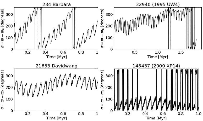
FIGURE 1. Time behavior of the resonant angle ϖ − ϖ₆ for an asteroid in a circulating orbit (top left panel), in a switching orbit (top right panel) in an antialigned orbit (bottom left panel) and in an aligned orbit (bottom right panel). Adapted from the Figure 1 of Carruba et al. (2022b).

Datasets with proper elements and labels for these four resonances are currently available in repositories listed in the cited articles, and at a GitHub repository prepared for this work. Such databases were designed, in most cases, for multi-class problems, with a 0 label for asteroids in circulating orbits, 1 for switching cases, and 2 for the librating cases. Here we will focus our attention on the use of imbalance learning to predict the labels of asteroids in the librating classes, which are the ones that are of most interest for asteroid dynamical studies. For this purpose, we converted the available databases into dual ones, for which 0 identifies orbits that are not in the librating class of interest, and 1 is associated with the relevant librating class.

Table 1 presents the number of asteroids in each class for the various problems, while Figure 2 shows the synthetic proper (a, sin(i)) distribution for the z₂ and aligned ν₆ databases, which are the two extreme cases of imbalance between class 0 and class 1. We chose to plot the data in the (a, sin(i)) plane rather than in the (a, e) domain because proper inclination is more stable on longer timescales than proper eccentricity. Proper inclination is a function of the angular momentum and of its z-component, while the proper eccentricity also depends on the orbital energy. Non-conservative forces can affect the orbital energy, but not the angular momentum. As a consequence, asteroid families are more recognizable in proper (a, sin(i)) domains. Here a denotes the proper semi-major axis of the asteroid orbit, and i represents the proper inclination of the orbital plane. Contrary to osculating orbital elements, proper elements are constants of the motion on timescales of the order of a few million years. Interested readers can refer to Knežević and Milani (2003) for information on obtaining synthetic proper elements. For some of the studied databases, such as the one for the aligned configuration of the ν₆ secular resonance, there is a severe imbalance between the two classes and one could expect to encounter the problems and limitations of conventional machine learning methods, as discussed in Section 1.

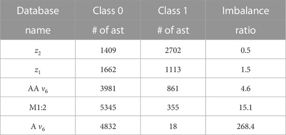
TABLE 1. We report the number of asteroids in class 0, class 1, and the imbalance ratios between class 0 and class 1 for the asteroid databases studied in this work. AA ν₆ stands for the antialigned configuration of this resonance, with oscillations of the resonant argument around the 180° equilibrium point, while A means aligned, with oscillations around the 0° equilibrium point.

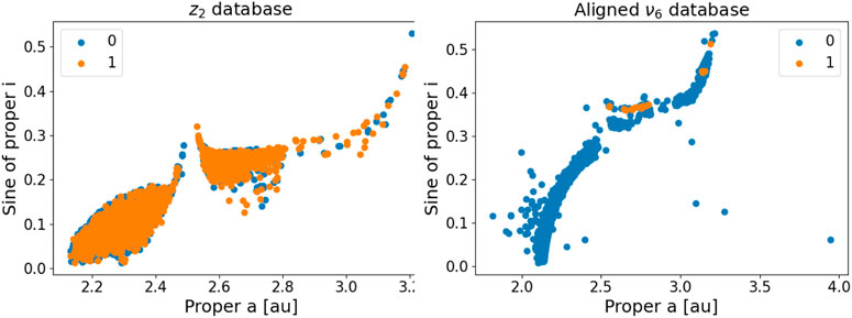
FIGURE 2. An (a, sin(i)) projection of the asteroids in the z₂ and aligned ν₆ databases.

2.2 Base models

After setting up the databases that we are going to study in this work with the procedure discussed in the previous section, we aim to identify the optimal machine learning (ML) method to fit each database. To test the efficiency of each method, we will use the area under curve score (AUC) of the receiver operating characteristic (ROC) curve. The ROC curve is a is a graphical representation of the performance of a binary classification model. It plots the True Positive Rate (TPR) on the y-axis and the False Positive Rate (FPR) on the x-axis. The true positive rate is defined as:

where the true positives are data correctly identified by the model to belong to the desired class, while false negatives are data miss-classified as belonging to the class of interest. Other used names for TPR are sensitivity or recall.

The false positive rate (FPR, hereafter) is defined as:

where false positives are outcomes where the model incorrectly predicts the positive class, and true negatives are data in the negative class correctly identified by the model. The plot displays the percentage of correct predictions for the positive class (y-axis) versus the percentage of errors for the negative class (x-axis). The best possible classifier would have a TPR of 1 and a FPR of 0. By analyzing the true positives and false positives for different threshold levels a curve that runs from the bottom left to the top right and bows toward the top left can be formed. This is known as the ROC curve. A classifier that is unable to distinguish between positive and negative classes will draw a diagonal line from a FPR of 0 to a TPR of 1 (coordinate (0,1)) or forecast all negative classes. Models indicated by points below this line have worse than no skill. The performance of a model can be quantitatively estimated using the ROC area under curve (ROC AUC). This is a score between 0.0 and 1.0, with 1.0 being the value for a perfect classifier. For the ROC AUC score we are using the default cut-off point in probability between the positive and negative classes at 0.5.

As an example of an ROC curve we display in Figure 3 the case of predictions from a no-skill classifier, which is unable to distinguish between positive and negative classes, and a Logistic Regression model Cox (1958), used to predict classes for a binary problem with equal weights for the two classes. Interested readers can find more details on how to produce this example in chapter 7 of Brownlee (2020). The logistic regression model had an ROC AUC of 0.90, while the no-skill model had a score of 0.50.

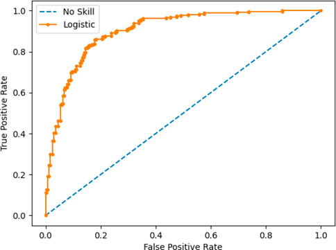
FIGURE 3. ROC Curve of a Logistic Regression Model and a no-skill classifier. Adapted from figure 7.1 of Brownlee (2020), available from Jason Brownlee, Imbalanced Classification with Python, https://machinelearningmastery.com/imbalanced-classification-with-python/, accessed 10 November 2022.

To identify the best-performing model and its optimal set of hyper-parameters, we used genetic algorithms. Genetic algorithms were first developed by Bremermann (1958) and popularized by Holland (1962). They are a search and optimization programming technique based on Darwin’s theory of species evolution, in which the strongest individual is favored, and their reproduction is more likely than that of others, forming a new generation. Using the methods codified by Chen et al. (2004), and following the procedure described by Carruba et al. (2021a) and Lourenço and Carruba (2022), we identified the best machine learning algorithms and the most appropriate combination of hyper-parameters for each considered database. Our results are summarized in Table 2, while in Section 1 of the supplementary materials we report the full set of hyper-parameters for each model. We use the ROC AUC score to assess the validity of each model. Since the methods are stochastic in nature, we applied each model ten times to provide an estimate of the ROC AUC score’s value and of its error, defined as the mean and the standard deviation of the ten outcomes, respectively. Errors were generally very small and of the order of 10^–3.

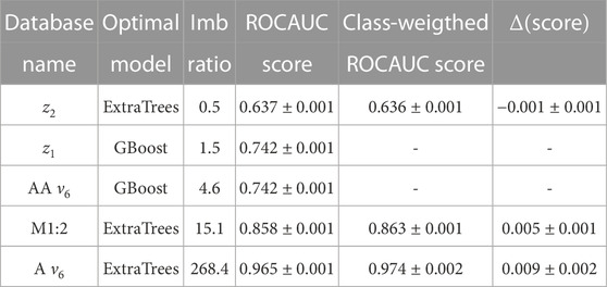
TABLE 2. The optimal machine learning model for the five datasets studied in this work (second column, GBoost stands for GradientBoosting). The third column shows the Imbalance ratio of the database. The fourth column displays the values of the ROC AUC score for the best-performing methods, with their errors. For tree-based methods, we displayed in the fifth column values of the ROC AUC score after the methods were optimized by assigning higher weights to the imbalanced classes.

Models that use the ExtraTrees classifier can be further optimized by assigning proper weights to each class. This method is called a cost-sensitive approach. We briefly mentioned the confusion matrix when we introduced the concept of ROC AUC score. For a binary classification problem, we can distinguish between the actual negatives and positives, and the predicted ones. The confusion matrix has the structure shown below:

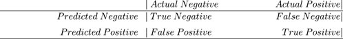
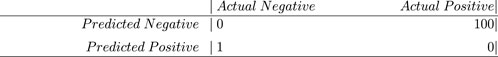
For imbalanced datasets, since there are much fewer members of class 1 than class 0, the cost of predicting a False Negative is much higher than that of predicting a False Positive. Failing to detect a real member of class 1 may produce a sample that is even more imbalanced than the original class. In contrast, predicting a False Positive has a smaller impact. This imbalance can be corrected by assigning different weights to False Negatives and False Positives. For example, in the case of a 1:100 ratio of examples in the minority class, we can define a cost matrix where the cost of a False Positive event is 1, while that of a False Negative is 100 as shown below:

Tree-based algorithms can automatically assign different weights to different classes based on the heuristic approach by selecting the option class_weight = “balanced.” We further optimized the tree-based algorithms for the z₂, M1:2, and aligned ν₆ databases, and our results are displayed in the fifth and sixth columns of Table 2. We define Δ(score) as the difference between the ROC AUC scores of the models with and without class weights. Its error is computed using standard error propagation formulas. We can see that Δ(score) depends on the imbalance ratio. It is negligible for the balanced z₂ dataset, and it is maximum for the more imbalanced aligned ν₆ database.

3 Imbalance correction methods: Results

Methods for correcting class imbalance depend on how they handle the minority and majority classes. Methods that increase the population of the minority class are classified as oversampling. Approaches that decrease the majority class are called undersampling. Finally, both oversampling and undersampling can be used at the same time.

For instance, in the random oversampling method examples from the minority class are randomly duplicated and added to the training dataset, until the minority class has the same number of members as the majority one. This is often referred to as the “minority class” sampling strategy. Random undersampling involves deleting random examples from the majority class to reduce the class imbalance, ideally until both classes have the same number of members. A more commonly used oversampling method is the Synthetic Minority Oversampling Technique, or SMOTE (Chawla et al., 2002). SMOTE works by picking instances in the feature space that are close together, drawing a line connecting the examples, and drawing a new sample at a position along that line.

To be specific, initially a random case from the minority class is picked and then, for that example, k of its nearest neighbors are determined (usually k = 5). A randomly determined neighbor is selected, and a new example is constructed in the feature space at a randomly chosen position between the two instances.

A commonly used undersampling method is Tomek Links, or simply Tomek (Tomek, 1976). The method is a modification of the condensed nearest-neighbor (CNN) approach Hart (1968). CNN is an undersampling strategy that finds a subset of samples that results in no loss in model performance, also known as a minimal consistent set. It is a subset that correctly classifies all of the remaining points in the sample set when used as a stored reference set for the k-nearest neighbors (KNN) rule Ghosh and Bandyopadhyay (2015). This is accomplished by enumerating the samples in the dataset and adding them to the store only if they cannot be accurately categorized by the store’s present contents. Tomek (1976) made two modifications to CNN, one of which is a method that selects pairs of samples, one from each class, that have the minimal Euclidean distance in feature space to each other. In a binary classification problem with classes 0 and 1, this means that a pair would have an example from each class and be closest neighbors throughout the dataset.

Examples of applications of both SMOTE and Tomek to the ν₆ antialigned database are shown in Figure 4. The first method oversamples the minority class so that it has the same number of objects as the majority one, while Tomek undersamples the majority class to reduce the imbalance.

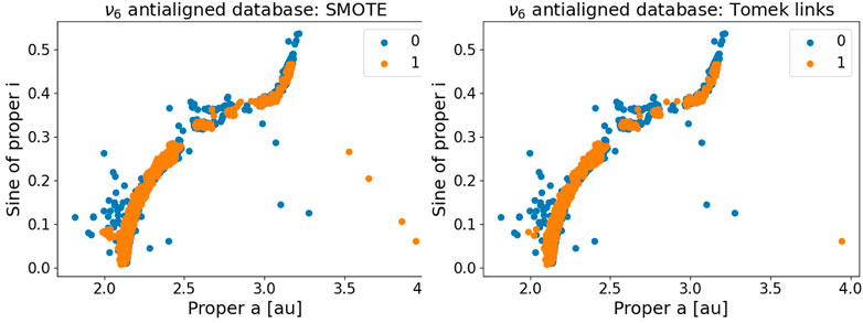
FIGURE 4. Left panel: application of SMOTE to the ν₆ antialigned database: Right panel: application of Tomek links to the same data.

Apart from SMOTE and Tomek, several other methods have been recently introduced and are available in the imblearn library (Lemaître et al. 2017), which we will use in this work. Among the oversampling approaches, we can mention Borderline SMOTE, Borderline SMOTE plus SVM, and ADASYN. Among the undersampling approaches, we also have Near Miss (versions 1, 2, and 3) Edited Nearest Neighbours, One Side Selection, and Neighbourhood Cleaning Rule. Finally, the most effective combinations of oversampling and undersampling are Random and Random, SMOTE plus Random, SMOTE plus Tomek, and SMOTE plus Edited Nearest Neighbours. To avoid making this text too long, we will not provide a detailed explanation of all these methods here. Interested readers can find more details on these methods in Brownlee (2020), and in Section 2 of the Supplementary materials.

Table 3 displays our results for the ν₆ aligned database, which is the most imbalanced among the ones considered in this work. Similar tables for the other datasets are presented in Section 3 of the supplementary materials. As expected, balanced databases, such as the z2 and z1 datasets, do not benefit from imbalance learning methodologies. In general, undersampling algorithms did not do well, with the three variations of the Near Miss methods, which retain instances of the majority class based on how far away the minority class data is from them, performing the worst. The combinations of random oversampling and undersampling, SMOTE oversampling, and SMOTE oversampling plus Tomek undersampling showed the greatest results for the three most unbalanced datasets, the antialigned nu6, M1:2, and aligned nu6. Their performance in terms of Δ(score) versus the Imbalance ratio is displayed in Figure 5. Imbalanced classification algorithms can provide an increase in performance of up to ≃ 1%.

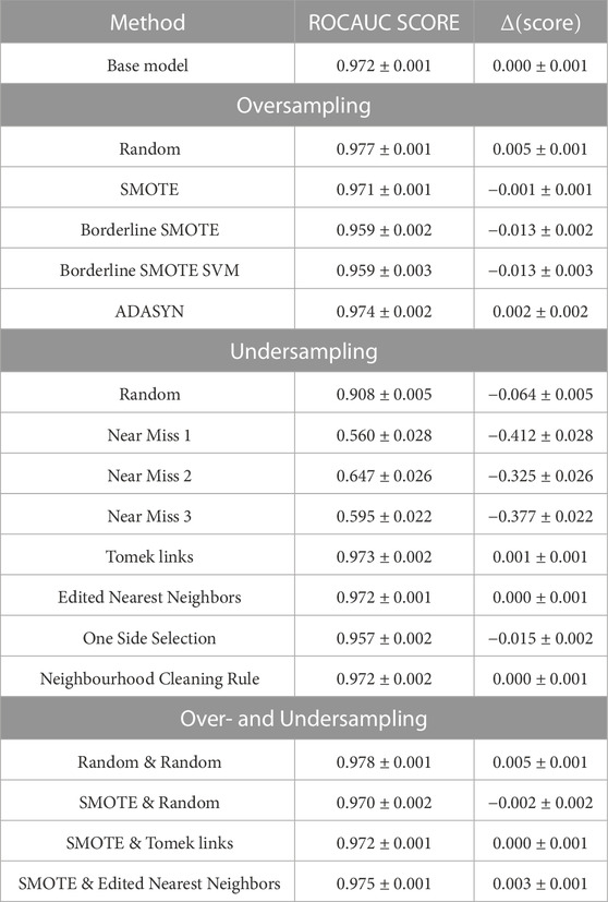
TABLE 3. Results of imbalanced models for the ν₆ aligned dual database (1: 268 imbalance).

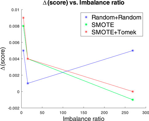
FIGURE 5. Dependence of the Δ(score) versus the Imbalance ratio for the three most successful models: a combination of Random oversampling and undersampling, SMOTE oversampling, and SMOTE oversampling plus Tomek undersampling.

4 Conclusion

In this work, we applied imbalanced classification methods to study five available datasets for asteroids interacting with four different resonances, namely, the z₂, z₁, M1:2, and ν₆. Firstly, we transformed the datasets from multi-labels to dual classes, with a label 1 assigned to asteroids in librating configurations, and a label 0 given to the rest, to allow the application of standard methods of imbalanced classification. Then, we used genetic algorithms to identify which machine learning methods, and what combination of their hyper-parameters, could best fit the data. For tree-based algorithms, a cost-sensitive approach was also used for further optimization. Finally, we tested various methods of oversampling, undersampling, or combinations of both, using the optimal models identified with the genetic algorithms.

Our findings show that cost-sensitive optimization methods should always be considered when feasable, since they either enhance the model’s performance or have no effect. Imbalanced classification methods are recommended for datasets with severe imbalance. Although each database is unique and should be studied independently to determine the most effective imbalance method, the experience gained in this study suggests that testing SMOTE oversampling plus Tomek undersampling, SMOTE oversampling, and Random oversampling and undersampling, in this order, could be a good strategy for dealing with imbalanced datasets for asteroids’ resonant problems. Testing these methods first could save considerable time and efforts for future studies in this area.

Data availability statement

All the original databases used in this work are publically available at links provided in the following references: Carruba et al. (2021b), Carruba et al. (2021a), Carruba et al. (2022b). A new GitHub repository with the codes and modified databases developed for this research is available at this link: https://github.com/valeriocarruba/Imbalanced_Classification_for_Resonant_Dynamics. Any additional data not found in these sources can be obtained from the first author upon reasonable request.

Author contributions

All authors contributed to the study conception and design. Material preparation, and data collection were performed by VC, ML, and SA. The first draft of the manuscript was written by VC and all authors commented on later versions of the manuscript. All authors read and approved the final manuscript. All authors contributed to the article and approved the submitted version.

Funding

We thank the Brazilian National Research Council (CNPq, grants 304168/2021-17 and 153683/2018-0) for supporting VC and BM research. ML is thankful for the support from the São Paulo Science Foundation (FAPESP, grant 2022/14241-9). GC acknowledge support by the Coordination of Superior Level Staff Improvement (CAPES) – Finance Code 001.

Acknowledgments

We are grateful to two reviewers for comments and suggestions that greatly improved the quality of this work. This is a publication from the MASB (Machine learning Applied to Small Bodies, https://valeriocarruba.github.io/Site-MASB/) research group. Questions regarding this paper can also be sent to the group email address: mlasb2021@gmail.com.

Conflict of interest

The authors declare that the research was conducted in the absence of any commercial or financial relationships that could be construed as a potential conflict of interest.

Publisher’s note

All claims expressed in this article are solely those of the authors and do not necessarily represent those of their affiliated organizations, or those of the publisher, the editors and the reviewers. Any product that may be evaluated in this article, or claim that may be made by its manufacturer, is not guaranteed or endorsed by the publisher.

References

Bremermann, H. J. (1958). The evolution of intelligence: The nervous system as a model of its environment. Seattle, Washington: University of Washington.
Brownlee, J. (2020). Imbalanced classification with Python: Choose better metrics, balance skewed classes, and apply cost-sensitive learning. San Juan, Puerto Rico: Machine Learning Mastery.
Carruba, V., Aljbaae, S., Caritá, G., Domingos, R. C., and Martins, B. (2022a). Optimization of artificial neural networks models applied to the identification of images of asteroids’ resonant arguments. Celest. Mech. Dyn. Astronomy 134, 59. doi:10.1007/s10569-022-10110-7
Carruba, V., Aljbaae, S., Domingos, R. C., and Barletta, W. (2021b). Artificial neural network classification of asteroids in the M1:2 mean-motion resonance with Mars. MNRAS 504, 692–700. doi:10.1093/mnras/stab914
Carruba, V., Aljbaae, S., Domingos, R. C., Huaman, M., and Martins, B. (2022b). Identifying the population of stable ν6 resonant asteroids using large data bases. MNRAS 514, 4803–4815. doi:10.1093/mnras/stac1699
Carruba, V., Aljbaae, S., and Domingos, R. C. (2021a). Identification of asteroid groups in the z1 and z2 nonlinear secular resonances through genetic algorithms. Celest. Mech. Dyn. Astronomy 133, 24. doi:10.1007/s10569-021-10021-z
Chawla, N. V., Bowyer, K. W., Hall, L. O., and Kegelmeyer, W. P. (2002). Smote: Synthetic minority over-sampling technique. J. Artif. Intell. Res. 16, 321–357. doi:10.1613/jair.953
Chen, P. W., Wang, J. Y., and Lee, H. (2004). “Model selection of SVMS using GA approach,” in 2004 IEEE International Joint Conference on Neural Networks (IEEE Cat. No.04CH37541), Budapest, Hungary, 25-29 July 2004, 2035–2040.
Cox, D. R. (1958). The regression analysis of binary sequences. J. R. Stat. Soc. Ser. B Methodol. 20, 215–232. doi:10.1111/j.2517-6161.1958.tb00292.x
Ghosh, D., and Bandyopadhyay, S. (2015). “A fuzzy citation-knn algorithm for multiple instance learning,” in 2015 IEEE International Conference on Fuzzy Systems (FUZZ-IEEE), Istanbul, Turkey, 02-05 August 2015. 1–8. doi:10.1109/FUZZ-IEEE.2015.7338024
Hart, P. (1968). The condensed nearest neighbor rule (corresp). IEEE Trans. Inf. Theory 14, 515–516. doi:10.1109/TIT.1968.1054155
Holland, J. H. (1962). Outline for a logical theory of adaptive systems. J. ACM 9, 297–314. doi:10.1145/321127.321128
Knežević, Z., and Milani, A. (2003). Proper element catalogs and asteroid families. Astronomy Astrophysics 403, 1165–1173. doi:10.1051/0004-6361:20030475
Lemaître, G., Nogueira, F., and Aridas, C. K. (2017). Imbalanced-learn: A python toolbox to tackle the curse of imbalanced datasets in machine learning. J. Mach. Learn. Res. 18, 1–5.
Lourenço, M. V. F., and Carruba, V. (2022). Genetic optimization of asteroid families’ membership. Front. Astronomy Space Sci. 9, 988729. doi:10.3389/fspas.2022.988729
Pedregosa, F., Varoquaux, G., Gramfort, A., Michel, V., Thirion, B., Grisel, O., et al. (2011). Scikit-learn: Machine learning in Python. J. Mach. Learn. Res. 12, 2825–2830.
Ribeiro, F., and Gradvohl, A. L. S. (2021). Machine learning techniques applied to solar flares forecasting. Astronomy Comput. 35, 100468. doi:10.1016/j.ascom.2021.100468
Keywords: machine learning, minor planets asteroids: general, artificial intelligence, data structure and algorithms, planetary science
Citation: Carruba V, Aljbaae S, Caritá G, Lourenço MVF, Martins BS and Alves AA (2023) Imbalanced classification applied to asteroid resonant dynamics. Front. Astron. Space Sci. 10:1196223. doi: 10.3389/fspas.2023.1196223
Received: 29 March 2023; Accepted: 26 April 2023;
Published: 11 May 2023.
Edited by:
Josep M. Trigo-Rodríguez, Spanish National Research Council (CSIC), SpainReviewed by:
Juan Rizos, Instituto de Astrofísica de Andalucía, SpainEvgeny Smirnov, Independent researcher, Barcelona, Spain
Copyright © 2023 Carruba, Aljbaae, Caritá, Lourenço, Martins and Alves. This is an open-access article distributed under the terms of the Creative Commons Attribution License (CC BY). The use, distribution or reproduction in other forums is permitted, provided the original author(s) and the copyright owner(s) are credited and that the original publication in this journal is cited, in accordance with accepted academic practice. No use, distribution or reproduction is permitted which does not comply with these terms.
*Correspondence: V. Carruba, valerio.carruba@unesp.br