Revisiting the Ground Magnetic Field Perturbations Challenge: A Machine Learning Perspective

1 Introduction

Horizontal magnetic field variations (dB_H/dt) derived from ground magnetometer recordings have been utilized commonly as a proxy for evaluating the risk that geomagnetically induced currents (GIC) present in different regions (e.g., Viljanen et al., 2001; Pulkkinen et al., 2015; Ngwira et al., 2018). GICs occur in ground-level conductors following an enhancement of the geoelectric field on the ground, usually in association with active geomagnetic conditions (Ngwira et al., 2015; Gannon et al., 2017), and have been known to cause damage to power transformers, corrode pipelines, and interfere with railway signals (Pirjola, 2000; Boteler, 2001; Pulkkinen et al., 2017; Boteler, 2019). As our society continues to become more “technology dependent” and as we enter a new cycle of intense geomagnetic activity during the ascending and maximum phases of solar cycle 25, having the appropriate tools to assess the risk GICs pose to different regions becomes urgently relevant (Oughton et al., 2019; Hapgood et al., 2021).

GIC levels are dependent on the characteristics of the system they affect as well as the environmental conditions, and unfortunately, measured GIC data are rarely available to the scientific community as they are either not monitored or the measurements restricted by power operator and therefore not made public. For this reason, variations of the measured ground magnetic field are commonly used as proxy to estimate the risk of GIC occurrence (Viljanen, 1998; Viljanen et al., 2001; Wintoft, 2005; Dimmock et al., 2020). These variations can be utilized to calculate the geoelectric field in regions where the ground conductivity profile is available (Love et al., 2018; Lucas et al., 2020; Gil et al., 2021).

In the past, many attempts have been made to forecast dB_H/dt with different degrees of success, using first-principles and empirical models (e.g., Tóth et al., 2014; Wintoft et al., 2015). However, comparisons are rarely made between models, in part because most models are not meant to be deployed for operational purposes, but also because models have different general forecasting objectives. The Geospace Environment Modeling (GEM) challenge (Pulkkinen et al., 2013) that ran during the years 2008–2012 tried to provide a direct comparison between models and to choose a model for real-time forecasting. It involved the entire space weather community in order to come up with a standardized method to test models against each other, and from there select a model to be transitioned into operation at NOAA (Pulkkinen et al., 2013).

Recently, machine learning empirical models have become more common thanks in part to the increased availability of data for training and the improvement of open-source machine learning tools (e.g. Keesee et al., 2020). Machine learning models present the advantage that, once trained, execution time is extremely low, and as such, they are able to deploy for real-time forecasting with extremely low computational cost. But while machine-learned models are able to forecast dB_H/dt or even GICs when data is available to different degrees of success, few attempts have been made to evaluate them on the grounds of established benchmarks. It is within that framework that we attempt to evaluate a series of machine learning models with the same metrics used by the GEM Challenge. In Section 2 we describe the GEM challenge in detail as well as the datasets we utilized and the models we developed. Section 3 presents the results of our models in the context of the GEM challenge metrics. In Section 4 we discuss the main challenges and lessons from our model development and comparisons. Finally, Section 5 presents our summary and conclusions.

2 Data and Methodology

The Geospace Environment Modeling (GEM) ground magnetic field perturbations challenge (“the GEM challenge”) consisted of a multi-year community effort that ran roughly between 2008 and 2011 with the objective of testing, comparing, and eventually delivering a model to be used at National Oceanic and Atmospheric Administration (NOAA) Space Weather Prediction Center (SWPC). The final results, description and evaluations of the different models that participated in the challenge are described in depth by Pulkkinen et al. (2013). The purpose of this study is to evaluate our machine learning based models using the same conditions and test on the same benchmarks, only deviating when an exact replication is not possible. The GEM challenge (and therefore the work presented here) consisted of forecasting the 1-min resolution of the horizontal component of ground magnetic field perturbations at several mid- and high-latitude stations. The horizontal component H is defined by

where E represents the east-west component, and N the north-south component in magnetic coordinates. The choice of forecasting the horizontal fluctuations is based on the assumption that it is the most important component for GIC occurrence (Pirjola, 2002). Although the GEM challenge involved a total of 12 different ground magnetometer stations during its different stages, the final evaluation presented in Pulkkinen et al. (2013) was performed only on 6 of them. Because the published scores are only available for those six stations, they will be the focus of this study. Table 1 lists the ground magnetometer stations, their code name and their magnetic latitude and longitude. Note that SNK replaced PBQ after 2007, so those data serve as a single location.

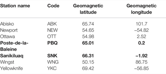
TABLE 1. Ground magnetometer stations used in this study and their location. Stations PBQ and SNK (in bold) are complementary as one replaces the other after the year 2007.

The GEM challenge proposed a unique and interesting evaluation mechanism. The models forecast four known geomagnetic storms during the testing period, and two extra storms were added as “surprise events” during the final evaluation. Table 2 presents the six storms used in the evaluation of the models. Our first deviation from the original challenge is that we are not evaluating our models on unknown storms—we have only calculated the final scores of the six storms after our training of the models was complete, and therefore we did not perform tuning of the models after the evaluation. The model output is the 1-min resolution horizontal component dB_H/dt predicted 1 minute ahead of time. This is counted from the time of arrival of the solar wind to the bow-shock nose, which involves a propagation from the L1 monitors. Once the forecast is done, the 1-min resolution predictions are reduced to obtain the maximum dB_H/dt value every 20 min. Each 20-min window prediction is then evaluated against four different thresholds set up at 18, 42, 66, and 90 nT/min. This approach turns the challenge into a classification problem, and a contingency table can be made for each of the thresholds counting true positives (hits), true negatives (no crossings), false positives (false alarms) and false negatives (misses). From this contingency table the values of probability of detection, probability of false detection, and the Heidke Skill Score are calculated. The definitions can be found in Pulkkinen et al. (2013). To obtain each model performance, the contingency tables are added by grouping the mid-latitude stations together (NEW, OTT, WNG) and the high-latitude stations together (ABK, PBQ/SNK, YKC) for each of the events and each of the thresholds.

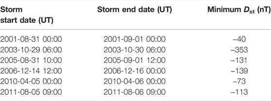
TABLE 2. Storms used for model evaluation.

2.1 Datasets and Pre-processing

For our study we have used the OMNI dataset obtained from the CDAWeb repository (https://cdaweb.gsfc.nasa.gov/pub/data/omni/omni_cdaweb/) at 1-min resolution. The OMNI database provides solar wind measurements obtained mostly from spacecraft located at the L1 Lagrangian point ($\sim 235R_E$ sunward of Earth) and then time-shifted to the magnetosphere’s bow shock nose (King and Papitashvili, 2005). We train our models to forecast 1-min ahead of the current time on the OMNI dataset, however, this is equivalent to a 20–40 min lead time if we were using real-time data, depending on the solar wind speed. The benefits of using the OMNI dataset for training is that it is a well validated dataset that is readily available for anyone to use with minimal work involved, and as such, it increases the reproducibility of the results. For our study, we used data between (and including) January 1995 and December 2019.

The OMNI dataset provides both plasma and magnetic field parameters, as well as some derived physical quantities. It suffers from having significant gaps which amount to around 20% of missing data in the plasma parameters and around 7% of missing data in the magnetic field. Further exploration of the data shows that most of the gaps are relatively small, and therefore we have performed a linear interpolation in the magnetic field parameters for gaps of up to 10 min, and we have performed a linear interpolation with no limit on time of the plasma parameters, to fill any possible gap. The remaining gaps, as determined by the missing magnetic field data, are dropped from the training dataset.

The ground magnetic field perturbations from the six different stations were obtained from the SuperMAG 1-min resolution database (https://supermag.jhuapl.edu/) with baseline removed (Gjerloev, 2012). The data availability is high for all the studied stations, although there are some significant gaps in the SNK/PBQ set around the time of the replacement in 2007–2008. We have decided not to perform any interpolation in the magnetic field components and therefore all missing data points are excluded from the training. For training, we use the N and E components to obtain dB_H/dt (Eq. 1) and also the MLT position of the observatories from the SuperMAG data.

Given the nature of the system we are trying to predict, one of the issues we have encountered is that the magnetic field fluctuations are heavily biased towards 0 nT/min. That is, during quiet times, the fluctuations are relatively low, and they amount for a sizable portion of the available dataset. On the contrary, during active times, the fluctuations can easily go up to the hundreds of nT/min at least for high-latitude stations. To reduce the bias, we have decided to reduce our training samples to only those times in which a geomagnetic storm is occurring. To do this, we have identified all geomagnetic storms in the 1995–2018 period with SYM-H $<-50$ nT and we have selected for training the period between ±12 h around the minimum SYM-H value. Figures 1A,B show a visual representation of the effect of using only storm-time data. As can be appreciated for both the mid-latitude NEW station and the high-latitude YKC station, the restriction to storm-time only reduces the training dataset to $\sim 10\%$ of its original size eliminating mostly small fluctuations. From the histogram, it can also be observed that—especially at high-latitudes—some strong fluctuations do occur outside of the storm-time. Those cases can prove interesting for analysis in the future, but will not be further discussed in the context of this work. It is important to note that the six storms considered for testing have been removed from the storm dataset. A list with the storm dates can be found in the Supplementary Material.

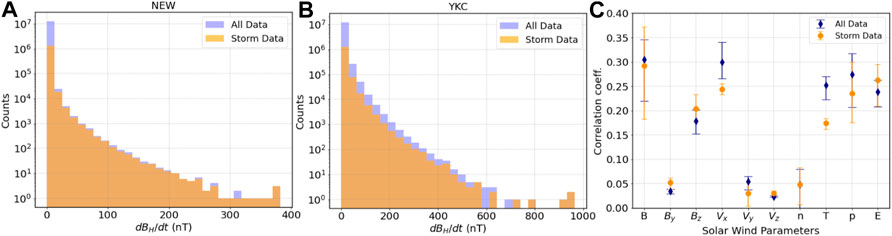
FIGURE 1. Histogram of dB_H/dt for all data between 1995 and 2019 (blue) and storm-only data (orange) for (A) the mid-latitude station NEW and (B) the high-latitude station YKC. (C) Correlation coefficient between different solar wind parameters and dB_H/dt for all data (blue) and storm-only data (orange). The symbol indicates the average of all six stations, and bars represent the range of the individual stations.

To train the models we have decided to use the following solar wind parameters: solar wind speed (Vx, Vy, Vz), interplanetary magnetic field (B_T, B_y, B_z), proton density, solar wind dynamic pressure, reconnection electric field (-VB_z), and proton temperature. Figure 1C shows the absolute value of the maximum correlation coefficient between dB_H/dt and the different solar wind parameters for the previous 60 min (i.e., max correlation of dB_H/dt(t) with param(t), param (t-1), etc). The symbol corresponds to the average correlation over the six stations used in this study, and the bar corresponds to the range of correlations. Here it is important to note that some parameters are most likely contributing significantly more to the training process than others. We have decided to keep them all on the basis that the models can support the amount of input parameters.

2.2 Models

For the evaluation of the GEM Challenge scores we used three different deep learning models: a feed-forward fully connected artificial neural network (ANN), a long short-term memory recurrent neural network (LSTM) and a convolutional neural network (CNN). The election of those particular models offers a continuation to our previous modelling attempts of dB_H/dt using neural networks (ANN + LSTM) (Keesee et al., 2020) as well as to test the capabilities of convolutional neural networks after they have shown promise for time series forecasting in different Space Weather applications (e.g., Collado-Villaverde et al., 2021; Siciliano et al., 2021; Smith et al., 2021). The development and training of the models was done using the TensorFlow-Keras framework for Python (Abadi et al., 2016) as well as the scikit-learn toolkit (Pedregosa et al., 2011). All models used in this study were trained by minimizing the mean square error. This optimization was done in each case using the Adam optimization algorithm. Further description of each model is given in the next sections.

2.2.1 Artificial Neural Network

Fully-connected feed-forward neural networks can capture temporal behavior (similar to a recurrent neural network) if the time history is embedded as a set of new features. In our case, we have built a 50-min time history of the selected solar wind parameters by creating new features (columns) in our dataset corresponding to the time-history of each parameter t − 1, … , t − 50 min. The time history length was determined purely by our maximum computational capabilities. This has resulted for our final model in an input array of 513 features. The network architecture contains four layers of 320–160–80–40 nodes. The activation function is the rectified linear unit (ReLU). To avoid overfitting, a dropout rate of 0.2 was added between the first and the second, and then between the second and third layers. The training ran for 300 epochs with the possibility of early stopping after 25 epochs of no improvement.

A consequence of embedding the time-history as extra features is that an independent array exists for each training point, and therefore we have trained our ANN model using a random 0.7/0.3 split, as opposed to the sequential split of the data that would be needed with a recurrent neural network. We have reasonably determined that the random split does not introduce data leakage to the model in our testing and that it resolves the bias introduced by the effect of different solar phases in the system. In this case, a more complex manual split of the data or a k-folds technique did not offer substantial improvement over the random split, which increased performance by $\sim 20\%$ compared to a sequential split.

2.2.2 Long-Short Term Memory

The Long-Short Term Memory (LSTM) neural network (Hochreiter and Schmidhuber, 1997) was developed as an alternative to solve the gradient vanishing problem of traditional recurrent networks by adding a “long memory.” This “memory” refers to the network’s ability to “remember” the state of previous cell states as well as previous outputs. The LSTM does this by using a series of gates, the first of which is the forget gate. The forget gate uses a sigmoid activation function, which varies between 0 and 1, to decide how much of the output from the previous cell output (t − 1) to feed to the next cell state (t). The input gate follows the forget gate and, as its name implies, determines what new information the cell state will receive. The first part of this gate consists of a tanh function, which uses a linear combination of the previous cell output and new input to the current cell, as well as a weight and bias factor. Another sigmoid function is then used to determine how much of the information from the tanh function will be input to the current cell state. The final gate used in the LSTM cell is the output gate, which uses another sigmoid function to determine how much information should be passed onto the next cell.

In our model, we used 100 cells in our LSTM layer, followed by two hidden dense layers using 1,000 and 100 nodes respectively. Each dense layer used ReLU activation. Dropout layers with weights of 0.2 were placed in between the hidden layers, and in between the final hidden layer and the output layer, to help prevent overfitting. The training ran for 100 epochs with the possibility of early stopping after 25 epochs of no improvement, and processed data with 60 min (determined by computational limitations) of time history embedded using the method described in Section 2.2.1.

2.2.3 Convolutional Neural Network

Convolutional Neural Networks (CNNs) were initially proposed as a method of detecting handwritten digits. They have since proved extraordinarily successful in a variety of image analysis problems (LeCun et al., 2015), and in recent years have shown promise in space weather forecasting (e.g., Collado-Villaverde et al., 2021; Siciliano et al., 2021; Smith et al., 2021). The CNN reads in a matrix all at once, and thus is not explicitly fed the time series information like the LSTM. The dimensions of CNN input array are (N, height, width, channels), where N is the number of sequences available for training, the height corresponds to the time history, and the width, the number of input features. The CNN is capable of analyzing multiple arrays in the same step. The channels dimension corresponds to the number of arrays to be analyzed at the same time, typically three for RGB color images. For this study we just have the CNN analyze one array per time step, so we set the number of channels equal to one. To keep some consistency between the LSTM and the CNN we used the same input parameters, time history, training data, and training/validation splits, so the input array has dimensions of (N, 60, 13, 1).

The CNN layer functions by using a matrix window called a kernel, which is smaller in size than the 2D input array being analyzed by the layer at step t. The kernel performs a matrix multiplication between a weight matrix the size of the kernel and a segment of the input array of the same size. The output is then put through the activation function (here ReLU), and the kernel window repeats the operation after moving to the next segment of the image. The length that it moves is defined by the stride. In this study, a kernel of size (1,2) and stride of one were used, resulting in overlapping kernel windows between parameters, but not between t and t − 1 for the same parameter. Padding, which is the process of adding columns of zeros to the ends of the array image to retain the initial image size, was used. A Pooling layer was used to reduce computational time in the models. The Pooling layer is a method of using a kernel window to move over the output of a CNN layer. Unlike the CNN layer, it does not perform a matrix multiplication using a weight matrix, it only extracts the maximum value in the kernel for the MaxPool, or the average in the kernel for the AveragePool. In this case a MaxPooling layer was used, the maximum value in the kernel window is taken, and the dimensions of the resulting image are reduced. In our case, the output of the CNN layer was of size (60, 13, 1). A 2 × 2 kernel window and a stride of (2,2) were used, and the resulting dimensions of the output array were (30, 6, 1). The flatten layer was used, which stacks the resulting 2D output from the Pooling layer into a 1D array that can be used as input to the Dense layers. Following the MaxPooling layer were two Dense Layers with 1,024 and 128 nodes, respectively, and dropout of 0.2 in between to help prevent overfitting. The model was trained for 100 epochs and early stopping was used after 25 epochs of no improvement.

3 Results

The results presented in this section correspond to those obtained with the “best” version of each model. Our process of optimization involved testing the use of different solar wind parameters, lengths of the solar wind time series, scalers, splits, loss functions, etc. However, a formal hyper-parameter tuning process such as a Grid Search was not performed. Since model optimization is a never-ending task, we expect to continue it in the future.

Each model (for each station) was trained to output 1-min resolution dB_H/dt values. The final evaluation of those models was done on the six different storms listed in Table 2. Figure 2 shows two of the six storms: 14 December 2006 (left) and 5 April 2010 (right). The rest of the storms can be found in the Supplementary Material. Panels (a-d) in Figure 2 show the main parameters of the solar wind for each storm: SYM-H index, solar wind speed (V_x) component, proton density and interplanetary magnetic field (IMF) B_z. Both geomagnetic storms are driven by interplanetary coronal mass ejections, with a sharp increase in solar wind speed associated with the arrival. It is somewhat expected that most chosen storms correspond to coronal mass ejections as the sudden storm commencement has been associated with larger fluctuations on the ground (e.g., Kappenman, 2003; Fiori et al., 2014; Rogers et al., 2020; Smith et al., 2021). Beyond that, both storms are significantly different in strength and in their proton density and IMF profiles. Figures 2E–J panels show the 1-min dB_H/dt measurement from the six different stations considered for this study (black). The three top stations (e-g) correspond to the mid-latitude stations while the bottom three (h-j) are the high-latitude stations. It can be seen that, in general, dB_H/dt spikes tend to scale with the strength of the storm, although peaks can significantly differ in timing and magnitude for stations at similar latitudes depending on their magnetic local time (MLT).

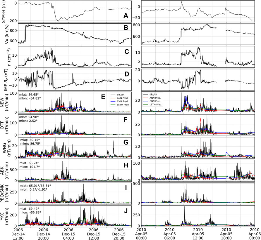
FIGURE 2. Solar wind parameters (A–D) and ground magnetometer dB_H/dt fluctuations as well as our model predictions (E–J) for all selected stations during the 14 December 2006 (left) and the 5 April 2010 (right) geomagnetic storms. Panels show (A) SYM-H index, (B) V_x, (C) proton density, (D) IMF B_z. Panels (E–J) show for each of the labeled stations the 1-min dB_H/dt fluctuations (black), and predictions from the ANN (red), CNN (blue) and LSTM (green) models.

The predictions in the lower panels are shown in red for the ANN, blue for the CNN and green for the LSTM. Those colors will remain associated with the respective models throughout the text. A quick overview of the predictions shown in Figure 2 indicates that the models are able to somewhat follow the trend of the enhanced activity, while missing most of the variability and spikes in dB_H/dt. A consequence of this is that all models severely under-predict the values unless the real measurements are relatively low. All three models do capture some of the spikes, or the overall increase of dB_H/dt during the storm-period. This is somewhat promising and let us speculate that the models can indeed follow the general evolution of the disturbance strength. At the moment, this is only true for certain stations and certain storms and further studies would be required to improve and evaluate the timing accuracy of the predictions.

Figure 3 shows the root mean square error (RMSE; smaller is better) and the coefficient of determination (R²; bigger is better) for each of the stations for the same storms shown in Figure 2. The rest of the storms can be found in the Supplementary Material. By itself, RMSE doesn’t allow us to evaluate the quality of the predictions. As can be clearly seen, different stations present markedly different results, with mid-latitude stations having lower RMSE than high-latitude stations due to the significantly lower magnetic fluctuations measured during geomagnetic storms. We can see in Figure 3 that RMSE values for the different models tend to obtain similar scores at mid-latitudes. At high-latitudes the CNN model performs slightly better than the other two models (by up to 10% depending on the station and the storm). The LSTM tends to perform similarly to the ANN in most of the stations for both storms, although the LSTM performance is slightly better, approaching and even surpassing the CNN performance on a few evaluations. The coefficient of determination (R²) parameter is less dependent on the magnitude of the fluctuations, and the results are relatively similar across all stations, suggesting that the models may have similar performance based on their solar wind inputs. From the figure, LSTM scores slightly better at mid-latitudes, while CNN performs better at high-latitudes. Still, the overall R² values are relatively low (0.1–0.3) and thus is hard to speculate on which model is better just from the pair of metrics shown.

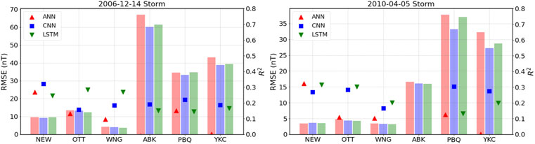
FIGURE 3. Root mean square errors (bars, left axis) and coefficient of determination R² (symbols, right axis) for each model and each station for the 14 December 2006 (left) and the 5 April 2010 (right) geomagnetic storms.

The 1-min resolution forecast proves similarly difficult for our models as it did in the original GEM challenge for the models that were evaluated (Pulkkinen et al., 2013). Therefore, a risk-assessment approach was introduced to evaluate whether the models would predict crossing at different thresholds using the maximum value of the predicted and real data every 20 min. Figure 4 shows the result of that transformation, with black indicating the real values, and colors indicating the prediction of the different models. Thresholds are drawn at 18, 42, 66 and 90 nT/min (dashed lines) and were selected following the requirements imposed on the models during the GEM Challenge (Pulkkinen et al., 2013). In the figure, the constant under-prediction of the models gets magnified by the drawing of the “upper envelope” of the fluctuations. This can be clearly seen in the 14 December 2006 results where the peak values at most stations are a factor of 10 or more higher than the predictions. This figure, however, does not necessarily indicate that the models perform poorly in the risk-assessment approach; as with the threshold evaluation, it is only important whether or not both the model and the original measurement cross a certain value. The relevant question for the metrics is whether both model and measurements are on the same side of the threshold or not. To do this, a contingency table is created for each storm, station, and threshold and the true positives (hits, H), true negatives (no crossing, N), false positives (false alarms, F), false negatives (missed crossing, M) are recorded.

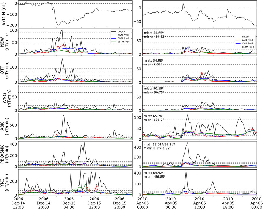
FIGURE 4. Maximum ground magnetic fluctuations every 20 min (black) and maximum predictions every 20 min for ANN (red), CNN (blue) and LSTM (green). Dashed black lines indicate the thresholds of prediction at 18, 42, 66, and 90 nT/min. From top to bottom, SYM-H index and the six magnetometer stations. The 14 December 2006 storm is shown to the left and the 5 April 2010 storm is shown to the right.

Following Pulkkinen et al. (2013) we transform the contingency table into probability of detection POD = H/(H + M), probability of false detection POFD = F/(F + N) and the Heidke Skill Score given by

The Heidke Skill Score weights the proportion of correct predictions obtained by the model against those that would be obtained purely by randomness. A positive score therefore indicates that the model performs better than chance. Figure 5 and Figure 6 show the probability of detection, probability of false detection and Heidke skill scores obtained at each station for the storms discussed in the previous figures. Figure 5 shows the values for the threshold of 18 nT/min. Despite the general under-prediction of the models, the probability of detecting the crossings at high-latitudes (ABK, PBQ, YKC) is $>0.5$ for all models in the 2006 storm and only slightly lower in the 2010 storm. At mid-latitudes the probability of detection is significantly lower for all stations, yet we see again a dominance of the CNN model for these particular cases. The probability of false detection is generally low at all stations and storms, although it is not quantified in this figure if that occurs because of the lack of real crossings over the threshold in that particular storm or not. Still, given the models’ consistent under-prediction problem, it is not reasonable to expect a significant number of false positives to contribute to this score. The Heidke Skill Score shows a larger spread even at the same station for different models, but consistently with the other metrics it seems to indicate a better performance of the models at high latitudes. A particularly interesting result is the extremely poor performance of the models in the station WNG, where none of the three models can get a single correct detection. This seems to be at least in part driven by the very small dB_H/dt values measured at that station for those storms.

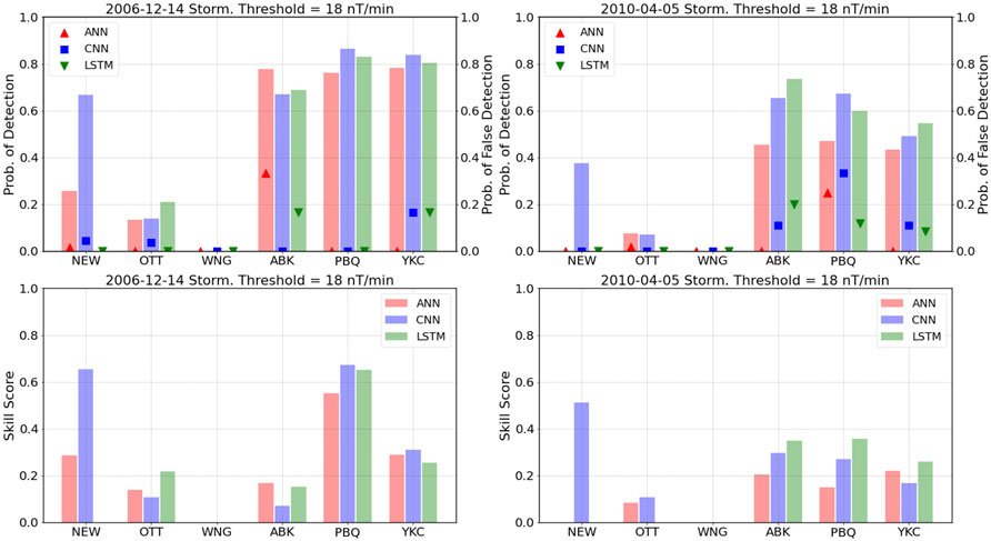
FIGURE 5. Top panels: Probability of detection (bars, left axis), probability of false detection (symbols, right axis). Bottom panels: Heidke skill score, calculated for the 18 nT/min threshold for each model and each station for the 14 December 2006 (left) and the 5 April 2010 (right) geomagnetic storms.

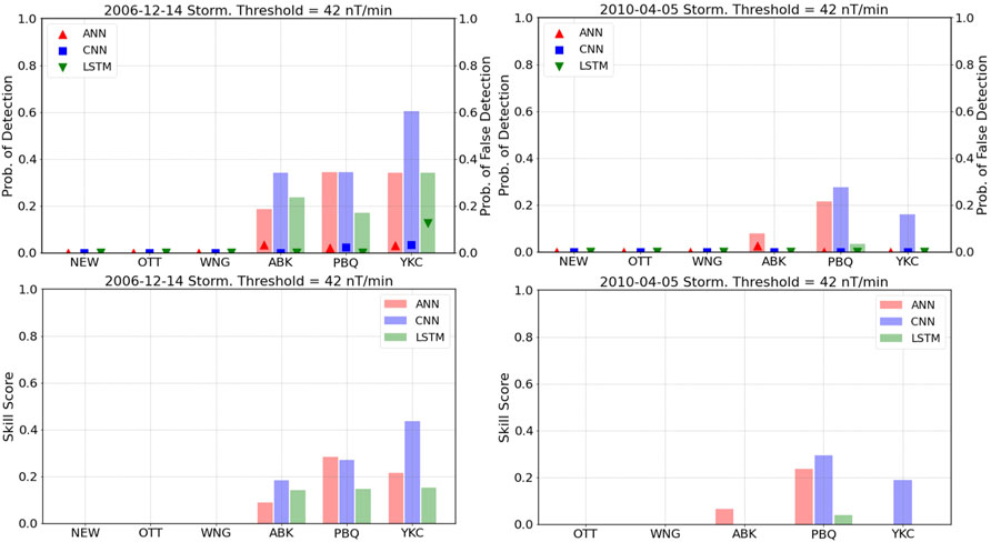
FIGURE 6. Top panels: Probability of detection (bars, left axis), probability of false detection (symbols, right axis). Bottom panels: Heidke skill score, calculated for the 42 nT/min threshold for each model and each station for the 14 December 2006 (left) and the 5 April 2010 (right) geomagnetic storms.

Figure 6, which shows the values for the threshold of 42 nT/min, shows a similar trend as Figure 5. The performance at high latitudes is varied depending on the station and the model, with the CNN model still outperforming the other two, but with results that are (at the very best) moderately good. The lack of a significant number of real crossings of the 42 nT/min threshold at mid-latitude stations makes evaluation of the models very difficult. Though a few crossings do occur, the models miss them. For that same reason we are not showing the individual results for the 66 nT/min and the 90 nT/min thresholds, although they are included in the Supplementary Material for the sake of completeness.

To properly compare with the GEM Challenge, we calculated the Heidke Skill Score by aggregating all the geomagnetic storms for all mid-latitude stations (WNG, NEW, OTT) and doing the same for the high-latitude stations (ABK, YKC, PBQ/SNK). This results in two scores for each threshold, one at high latitudes and one at mid-latitudes. Figure 7 shows the results obtained by each of the models at mid-latitudes (top panel) and high latitudes (bottom panel). From the figure, we can note that the final scores are generally consistent with the individual scores obtained in the previous figures (and with those not shown in the manuscript). It is clear that the model that uses a CNN outperforms the other two consistently at high-latitudes, for the first three thresholds. However, at mid-latitudes it is the LSTM model that performs the best, even holding some predictive power (i.e., HSS positive) at the 90 nT/min threshold. A comparison against the models shown by Pulkkinen et al. (2013) would indicate that the CNN and LSTM models outperform all the GEM challenge models at high latitudes for the lowest two thresholds but do a bit worse than the top performer (Space Weather Modeling Framework-SWMF) for the highest two. At mid-latitudes, however, even the LSTM model is outperformed by most of the GEM Challenge models, indicating that our models do present a different behavior at mid-latitudes and high latitudes, even beyond the differences in the scores which can be attributed to many causes.

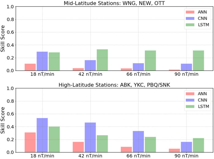
FIGURE 7. Cumulative Heidke Skill Score “GEM score” calculated by adding the contingency tables of all storms and all stations at mid (top) or high (bottom) latitudes for all three models and four thresholds.

4 Discussion

The development of machine-learning models to forecast 1-min ground magnetometer fluctuations (dB_H/dt) and our benchmark against the set of metrics previously used in similar models during the GEM Challenge for ground magnetic perturbations presented several interesting challenges, and therefore we have learned important lessons from the process. In the next sections we discuss a few of the most important points regarding the evaluation of the models and the improvements that need to be made moving forward.

4.1 The 30 October 2003 Storm

Out of the events selected for evaluation, perhaps the most interesting is the storm that occurred on 30 October 2003. This storm is the third largest storm recorded in the high resolution OMNI dataset (1995-present). It is reasonable to expect modelers to test the models on such extreme event. This storm, however, presents a series of challenges for our models, the most important being that there are no high resolution plasma parameters available during most of the storm due to a saturation of the instrument on-board the ACE spacecraft (Skoug, 2004). For our model evaluation of the 2003 storm, we used a procedure similar to that described by Pulkkinen et al. (2013) which involved the use of low-resolution (1-h) ACE data to reconstruct the plasma parameters and 4-s resolution data for the interplanetary magnetic field. The data was then propagated to the bow-shock nose to make it consistent with OMNI data. Figure 8 (left) shows the reconstructed solar wind data re-sampled at 1-min resolution. The only data that could not be reconstructed are solar wind speed V_y and V_z which are shown as straight lines connecting last known values (linear interpolation).

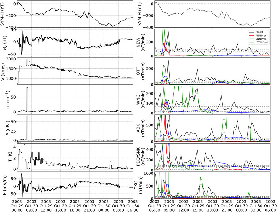
FIGURE 8. Solar wind parameters (left) and 20-min window ground magnetometer data and predictions (right) for the 30 October 2003 geomagnetic storm. From top to bottom (left) SYM-H index, IMF B_z, proton speed, proton density, dynamic pressure, temperature and electric field. From top to bottom (right) SYM-H index, and all six ground magnetometer stations showing 20-min window maximum values of real measurements (black), ANN model (red), LSTM model (green), and CNN model (blue).

Figure 8 (right) shows the prediction of the models for the different stations during the 30 October 2003 storm. Here, one of the main difficulties when training machine-learning models becomes evident: their poor ability to extrapolate to unseen data. It can be seen that the models behave in strange different ways. All three of the models respond to the sudden increase in proton density at the beginning of the evaluated timespan, but the models’ predictions differ significantly afterwards. For example, the ANN predictions go to zero following the initial spike, thus missing most of the strong fluctuations. The CNN model, although troubled to produce a strong prediction, seems to at least be robust enough to follow a pattern of prediction similar to what it would predict in different storms. Finally, the LSTM model predicts huge spikes in at least two stations. Fine-tuning a model to get good predictions on extreme (and unseen) data was not among the goals we set for this work, but it is something that we will consider moving forward.

4.2 Metrics

The Heidke Skill Score (HSS) was the main metric used here for comparison with the GEM challenge. The main reason for its use was that it was also their metric of choice, and as such was the simpler choice. We believe that the use of only one metric to evaluate a model is restrictive, as it provides only a glimpse into the strengths and weaknesses of that model. For example, the HSS (Equation 2) contains a series of products or sums between elements of the contingency table. This requires a variety of table elements to produce a meaningful score. During the process of model evaluation, the most intense storm in the testing suite, the 2003 Halloween storm, had a large percentage of missing data, meaning the model evaluation was only done on a portion of the storm where data was available. This portion of storm data was completely above the lowest (18 nT/min) threshold. The model, recognizing the intensity of the storm, predicted over the threshold for the same time period. This resulted in the H (hits) element of the table being the only one populated, as all of the predictions and real data were over the lowest threshold, ideally a perfect model. However, because only one element of the table was nonzero, we get zeros in both the numerator and denominator of the HSS, producing a NaN value in our evaluation. Similarly, in the evaluation of the 2003 storm, the PBQ station had an almost perfect prediction in terms of being all hits for the 18 nT/min threshold. However, while the proportion of hits was very high, there was one false negative. Because there were only two elements of the table represented, but they are in different terms of the numerator, we get a result of zero for the HSS. A score of zero is supposed to be akin to 50–50 random chance model; however, with a hit-to-false-negative proportion of 13:1 for this particular storm, that is obviously not the case, showing that the HSS does not do justice to the skill of the model. Thus, it is important to consider multiple metrics when validating or comparing models. Liemohn et al. (2021) provides an overview of numerous metrics, and Welling et al. (2018) recommends adding a Frequency Bias metric to those used by Pulkkinen et al. (2013) for assessment of ground magnetic field perturbations.

It is also important to consider that out of the six storms evaluated for the six ground magnetometer stations, the 30 October 2003 storm is the only storm that provides a high number of crossings above the higher three thresholds. This is also discussed in Pulkkinen et al. (2013) because it heavily impacts the overall HSS score of a model depending on whether the model can effectively predict fluctuations that are large enough to cross over those thresholds. In our case, the ANN model that fails to predict the 2003 storm at all, sees its HSS tremendously affected when compared against the other two models, even if they are all similar in performance for the remaining of the geomagnetic storms evaluated.

4.3 Training and Testing

One of the reasons to replicate an existing community effort is that we wanted to benchmark our model results against known baseline models. In doing so, we have made choices that may or may not be the optimal choices for a machine learning model. A good example is the 2003 storm, which would be ideally used for training instead of for testing given its unique nature in the existing dataset (and that we will use when the models move into operational real-time forecast). As mentioned before, it is understandable that modelers may want to test using extreme events, as opposed to machine-learning practices where extreme events can help models perform better. However, in the future, it may be worth exploring new events for testing, such as those already proposed by Welling et al. (2018).

Another important aspect not addressed in detail here is the choice of the target parameter. Following the GEM challenge we focused on the 1-min resolution dB_H/dt values, and then reprocessed those predictions to obtain the maximum value every 20-min, which is what was finally used for the actual evaluation. While a 20 or 30 min window of prediction is probably a reasonable timespan in which to raise warnings when a model is operational, the way the model was proposed, it is not actively creating predictions that far into the future but rather 1-min ahead (plus the time of propagation from L1), which can lead to confusion. In the future, we plan to try different types of forecasts, such as doing a direct prediction of the maximum value of the fluctuations over a determined time window.

5 Summary and Conclusion

We have revisited the ground magnetic field perturbations challenge “GEM Challenge” using deep learning models for our evaluation: a feed forward neural network (ANN), a convolutional neural network (CNN) and a long short-term memory recurrent network (LSTM). We followed the same procedure set by the original challenge, including the forecast of 1-min resolution dB_H/dt values, followed by a conversion to a “maximum of” in 20-min windows. We then evaluated our models by creating a contingency table for thresholds of 18, 42, 66 and 90 nT/min. The metrics created from these contingency tables were probability of detection, probability of false detection and the Heidke Skill Score, which we used to evaluate our models at six ground magnetometer stations, three mid-latitude and three high-latitude, over six different geomagnetic storms. We finally calculated an overall score by aggregating storms at mid-latitude stations and also at high-latitude stations.

Overall, we found that the machine-learning models we developed tend to perform similarly or slightly worse compared against the models presented by Pulkkinen et al. (2013), with scores that would situate them roughly in the middle of all the models they tested. Pulkkinen et al. (2013) does not present exact numbers, so those need to be inferred from their figures. For example, our models perform poorly for the 18 nT/min threshold at mid-latitudes compared to all models discussed there. On the other hand, two of our models (CNN, LSTM) outperform all but the two top models at high-latitude for the same threshold. At the 42 nT/min threshold, our models (LSTM at mid-lat, CNN at high-lat) would outperform all but the top model presented there. There are several reasons for such results, including difficulties in predicting the 30 October 2003 geomagnetic storm, which is a unique and extreme case that causes machine learning training to predict poorly. Out of the three models we tested, the CNN did consistently better than the other two.

The machine-learning models we used here have a few advantages over traditional simulations such as the minimal computational requirements they need for training, and to be run in real-time. Most of our models have been trained in machines of moderate computational power, and more importantly can provide real-time predictions on a desktop computer. This allows for great flexibility in the design of models and quick iteration between different algorithms as they become available. Here we used an LSTM, CNN, and even an ANN model for their capability to capture the time-history of the time series used as an input. We consider that any machine learning model capable of capturing the temporal evolution of the target parameter is worth exploring and could be used in the future. We plan in the future to continue exploring models of this type, with the intention of moving into real-time forecasting.

Data Availability Statement

Publicly available datasets were analyzed in this study. This data can be found here: OMNI Dataset: https://cdaweb.gsfc.nasa.gov/pub/data/omni/SuperMAg Dataset: https://supermag.jhuapl.edu/ACE Dataset: http://www.srl.caltech.edu/ACE/ASC/level2/index.html.

Author Contributions

VP contributed to conception and design of the study, data preparation, model development and analysis, interpretation of results, and writing. AK contributed to design of the study, interpretation of results, data preparation, writing and general guidance. MC and RM contributed to model development, analysis, interpretation, and assisted with writing. JJ contributed to model development and methodology design. CN and HC contributed with design of the study and overall discussion. All authors contributed to manuscript revision and read and approved the submitted version.

Funding

This work is supported by NSF Award 1920965. CN was supported through NASA Grant Award 80NSSC-20K1364 and NSF Grant Award AGS-2117932.

Conflict of Interest

The authors declare that the research was conducted in the absence of any commercial or financial relationships that could be construed as a potential conflict of interest.

Publisher’s Note

All claims expressed in this article are solely those of the authors and do not necessarily represent those of their affiliated organizations, or those of the publisher, the editors and the reviewers. Any product that may be evaluated in this article, or claim that may be made by its manufacturer, is not guaranteed or endorsed by the publisher.

Acknowledgments

We thank all members of the MAGICIAN team at UNH and UAF that participated in the discussions leading to this article. We also thank the OMNIWeb, SuperMAG and ACE teams for providing the data.

Supplementary Material

The Supplementary Material for this article can be found online at: https://www.frontiersin.org/articles/10.3389/fspas.2022.869740/full#supplementary-material

References

Abadi, M., Agarwal, A., Barham, P., Brevdo, E., Chen, Z., Citro, C., et al. (2016). TensorFlow: Large-Scale Machine Learning on Heterogeneous Distributed Systems. arXiv:1603.04467 [cs].
Boteler, D. H. (2019). A 21st Century View of the March 1989 Magnetic Storm. Space Weather 17, 1427–1441. doi:10.1029/2019SW002278
Boteler, D. H. (2001). “Space Weather Effects on Power Systems,” in Geophysical Monograph Series (Washington, D. C.: American Geophysical Union), 347–352. doi:10.1029/GM125p0347
Collado‐Villaverde, A., Muñoz, P., and Cid, C. (2021). Deep Neural Networks with Convolutional and LSTM Layers for SYM‐H and ASY‐H Forecasting. Space Weather 19, e2021SW002748. doi:10.1029/2021SW002748
Dimmock, A. P., Rosenqvist, L., Welling, D. T., Viljanen, A., Honkonen, I., Boynton, R. J., et al. (2020). On the Regional Variability of d B/d t and its Significance to GIC. Space Weather 18, e2020SW002497. doi:10.1029/2020SW002497
Fiori, R. A. D., Boteler, D. H., and Gillies, D. M. (2014). Assessment of GIC Risk Due to Geomagnetic Sudden Commencements and Identification of the Current Systems Responsible. Space Weather 12, 76–91. doi:10.1002/2013SW000967
Gannon, J. L., Birchfield, A. B., Shetye, K. S., and Overbye, T. J. (2017). A Comparison of Peak Electric Fields and GICs in the Pacific Northwest Using 1‐D and 3‐D Conductivity. Space Weather 15, 1535–1547. doi:10.1002/2017SW001677
Gil, A., Berendt-Marchel, M., Modzelewska, R., Moskwa, S., Siluszyk, A., Siluszyk, M., et al. (2021). Evaluating the Relationship between Strong Geomagnetic Storms and Electric Grid Failures in Poland Using the Geoelectric Field as a GIC Proxy. J. Space Weather Space Clim. 11, 30. doi:10.1051/swsc/2021013
Gjerloev, J. W. (2012). The SuperMAG Data Processing Technique. J. Geophys. Res. Space Phys. 117, A09213. doi:10.1029/2012ja017683
Hapgood, M., Angling, M. J., Attrill, G., Bisi, M., Cannon, P. S., Dyer, C., et al. (2021). Development of Space Weather Reasonable Worst‐Case Scenarios for the UK National Risk Assessment. Space Weather 19, e2020SW002593. doi:10.1029/2020SW002593
Hochreiter, S., and Schmidhuber, J. (1997). Long Short-Term Memory. Neural Comput. 9, 1735–1780. doi:10.1162/neco.1997.9.8.1735
Kappenman, J. G. (2003). Storm Sudden Commencement Events and the Associated Geomagnetically Induced Current Risks to Ground-Based Systems at Low-Latitude and Midlatitude Locations. Space Weather 1, 1016. doi:10.1029/2003sw000009
Keesee, A. M., Pinto, V., Coughlan, M., Lennox, C., Mahmud, M. S., and Connor, H. K. (2020). Comparison of Deep Learning Techniques to Model Connections between Solar Wind and Ground Magnetic Perturbations. Front. Astron. Space Sci. 7, 550874. doi:10.3389/fspas.2020.550874
King, J. H., and Papitashvili, N. E. (2005). Solar Wind Spatial Scales in and Comparisons of Hourly Wind and ACE Plasma and Magnetic Field Data. J. Geophys. Res. 110, A02104. doi:10.1029/2004JA010649
LeCun, Y., Bengio, Y., and Hinton, G. (2015). Deep Learning. Nature 521, 436–444. doi:10.1038/nature14539
Liemohn, M. W., Shane, A. D., Azari, A. R., Petersen, A. K., Swiger, B. M., and Mukhopadhyay, A. (2021). RMSE is Not Enough: Guidelines to Robust Data-Model Comparisons for Magnetospheric Physics. J. Atmos. Sol.-Terr. Phys. 218, 105624. doi:10.1016/j.jastp.2021.105624
Love, J. J., Lucas, G. M., Kelbert, A., and Bedrosian, P. A. (2018). Geoelectric Hazard Maps for the Mid-Atlantic United States: 100 Year Extreme Values and the 1989 Magnetic Storm. Geophys. Res. Lett. 45, 5–14. doi:10.1002/2017GL076042
Lucas, G. M., Love, J. J., Kelbert, A., Bedrosian, P. A., and Rigler, E. J. (2020). A 100‐Year Geoelectric Hazard Analysis for the U.S. High‐Voltage Power Grid. Space Weather 18, e2019SW002329. doi:10.1029/2019SW002329
Ngwira, C. M., Pulkkinen, A. A., Bernabeu, E., Eichner, J., Viljanen, A., and Crowley, G. (2015). Characteristics of Extreme Geoelectric Fields and Their Possible Causes: Localized Peak Enhancements. Geophys. Res. Lett. 42, 6916–6921. doi:10.1002/2015GL065061
Ngwira, C. M., Sibeck, D., Silveira, M. V. D., Georgiou, M., Weygand, J. M., Nishimura, Y., et al. (2018). A Study of Intense Local dB/dt Variations during Two Geomagnetic Storms. Space Weather 16, 676–693. doi:10.1029/2018SW001911
Oughton, E. J., Hapgood, M., Richardson, G. S., Beggan, C. D., Thomson, A. W. P., Gibbs, M., et al. (2019). A Risk Assessment Framework for the Socioeconomic Impacts of Electricity Transmission Infrastructure Failure Due to Space Weather: An Application to the United Kingdom. Risk Anal. 39, 1022–1043. doi:10.1111/risa.13229
Pedregosa, F., Varoquaux, G., Gramfort, A., Michel, V., Thirion, B., Grisel, O., et al. (2011). Scikit-Learn: Machine Learning in Python. J. Mach. Learn. Res. 12, 2825–2830.
Pirjola, R. (2000). Geomagnetically Induced Currents during Magnetic Storms. IEEE Trans. Plasma Sci. 28, 1867–1873. doi:10.1109/27.902215
Pirjola, R. (2002). Review on the Calculation of Surface Electric and Magnetic Fields and of Geomagnetically Induced Currents in Ground-Based Technological Systems. Surv. Geophys. 23, 71–90. doi:10.1023/A:1014816009303
Pulkkinen, A., Bernabeu, E., Eichner, J., Viljanen, A., and Ngwira, C. (2015). Regional-Scale High-Latitude Extreme Geoelectric Fields Pertaining to Geomagnetically Induced Currents. Earth Planet Sp. 67, 93. doi:10.1186/s40623-015-0255-6
Pulkkinen, A., Bernabeu, E., Thomson, A., Viljanen, A., Pirjola, R., Boteler, D., et al. (2017). Geomagnetically Induced Currents: Science, Engineering, and Applications Readiness. Space Weather 15, 828–856. doi:10.1002/2016SW001501
Pulkkinen, A., Rastätter, L., Kuznetsova, M., Singer, H., Balch, C., Weimer, D., et al. (2013). Community-Wide Validation of Geospace Model Ground Magnetic Field Perturbation Predictions to Support Model Transition to Operations. Space Weather 11, 369–385. doi:10.1002/swe.20056
Rogers, N. C., Wild, J. A., Eastoe, E. F., Gjerloev, J. W., and Thomson, A. W. P. (2020). A Global Climatological Model of Extreme Geomagnetic Field Fluctuations. J. Space Weather Space Clim. 10, 5. doi:10.1051/swsc/2020008
Siciliano, F., Consolini, G., Tozzi, R., Gentili, M., Giannattasio, F., and De Michelis, P. (2021). Forecasting SYM‐H Index: A Comparison between Long Short‐Term Memory and Convolutional Neural Networks. Space Weather 19, e2020SW002589. doi:10.1029/2020SW002589
Skoug, R. M. (2004). Extremely High Speed Solar Wind: 29-30 October 2003. J. Geophys. Res. 109, A09102. doi:10.1029/2004JA010494
Smith, A. W., Forsyth, C., Rae, I. J., Garton, T. M., Bloch, T., Jackman, C. M., et al. (2021). Forecasting the Probability of Large Rates of Change of the Geomagnetic Field in the UK: Timescales, Horizons, and Thresholds. Space Weather 19, e2021SW002788. doi:10.1029/2021SW002788
Tóth, G., Meng, X., Gombosi, T. I., and Rastätter, L. (2014). Predicting the Time Derivative of Local Magnetic Perturbations. J. Geophys. Res. Space Phys. 119, 310–321. doi:10.1002/2013JA019456
Viljanen, A., Nevanlinna, H., Pajunpää, K., and Pulkkinen, A. (2001). Time Derivative of the Horizontal Geomagnetic Field as an Activity Indicator. Ann. Geophys. 19, 1107–1118. doi:10.5194/angeo-19-1107-2001
Viljanen, A. (1998). Relation of Geomagnetically Induced Currents and Local Geomagnetic Variations. IEEE Trans. Power Deliv. 13, 1285–1290. doi:10.1109/61.714497
Welling, D. T., Ngwira, C. M., Opgenoorth, H., Haiducek, J. D., Savani, N. P., Morley, S. K., et al. (2018). Recommendations for Next‐Generation Ground Magnetic Perturbation Validation. Space Weather 16, 1912–1920. doi:10.1029/2018SW002064
Wintoft, P. (2005). Study of the Solar Wind Coupling to the Time Difference Horizontal Geomagnetic Field. Ann. Geophys. 23, 1949–1957. doi:10.5194/angeo-23-1949-2005
Keywords: geomagnetically induced currents, deep learning, ground magnetic disturbance, space weather, neural network
Citation: Pinto VA, Keesee AM, Coughlan M, Mukundan R, Johnson JW, Ngwira CM and Connor HK (2022) Revisiting the Ground Magnetic Field Perturbations Challenge: A Machine Learning Perspective. Front. Astron. Space Sci. 9:869740. doi: 10.3389/fspas.2022.869740
Received: 04 February 2022; Accepted: 04 May 2022;
Published: 25 May 2022.
Edited by:
Peter Wintoft, Swedish Institute of Space Physics, SwedenReviewed by:
Simon Wing, Johns Hopkins University, United StatesStefano Markidis, KTH Royal Institute of Technology, Sweden
Copyright © 2022 Pinto, Keesee, Coughlan, Mukundan, Johnson, Ngwira and Connor. This is an open-access article distributed under the terms of the Creative Commons Attribution License (CC BY). The use, distribution or reproduction in other forums is permitted, provided the original author(s) and the copyright owner(s) are credited and that the original publication in this journal is cited, in accordance with accepted academic practice. No use, distribution or reproduction is permitted which does not comply with these terms.
*Correspondence: Victor A. Pinto, victor.pinto@gmail.com