Orbit Design for LUMIO: The Lunar Meteoroid Impacts Observer
 Ana M. Cipriano
 Diogene A. Dei Tos
 Francesco Topputo
- 1Astrodynamics and Space Missions, Delft University of Technology, Delft, Netherlands
- 2Department of Aerospace Science and Technology, Politecnico di Milano, Milan, Italy
The Lunar Meteoroid Impacts Observer, or LUMIO, is a space mission concept awarded winner of ESA's SysNova Competition “Lunar CubeSats for Exploration,” and as such it is now under consideration for future implementation by the Agency. The space segment foresees a 12U CubeSat, placed at Earth–Moon L2, equipped with an optical instrument, the LUMIO-Cam, which is able to spot the flashes produced by impacts of meteoroids with the lunar surface. In this paper, the work undertaken to design the baseline orbit of LUMIO is documented. The methodology is thoroughly described, both in qualitative and quantitative terms, in support to the mission analysis trade-off activities. The baseline solution is presented with evidence to support the orbit design.
1. Introduction
1.1. Scientific Relevance
Near-Earth Objects (NEOs) are asteroids or comets with a perihelion of < 1.3 astronomical units (AU), whose orbits encounter the Earth neighborhood. In the Minor Planet Center database1, the vast majority of NEOs are classified as Near-Earth Asteroids (NEAs), while only a small fraction are classified as Near-Earth Comets (NECs). Both types of minor bodies (NEAs and NECs) are remnant debris of the solar system formation and contain clues that can contribute to the understanding of the composition of planets. The relatively easier accessibility of NEOs, when compared to deep-space asteroids, represents a valuable opportunity to improve the understanding of the solar system at an affordable cost.
Impacts due to Near-Earth Objects could cause a devastating humanitarian crisis and potentially the extinction of the human race. While the probability of such an event is low, the outcome is so catastrophic that it is imperative to invest resources to mitigate them. The largest impact event recorded in history is attributed to a NEO impact, is know as the Tunguska event and occurred in 1908. According to Brown et al. (2013), an event like this could occur every 100 years. The second largest airburst event recorded occurred in 2013 in the Russian city of Chelyabinsk, causing damages over a 120 km radius and at least 374 injured (Popova et al., 2013). Telescopic surveys detect NEOs whose size ranges from slightly larger than 1 km down to tens of meters (Koschny and McAuliffe, 2009), but there are few direct methods for monitoring the sub-meter meteoroid population. Serendipitous monitoring of atmospheric explosions due to airbursts of large meteoroids are also being undertaken.
Meteoroids are small Sun-orbiting fragments of asteroids and comets, whose sizes range from micrometers to meters and masses from 10−15 to 104 kg (Ceplecha et al., 1998). Their formation is a consequence of asteroids colliding with each other or with other bodies, comets releasing dust particles when close to the Sun, and minor bodies shattering into individual fragments. Meteoroids are hardly detectable even with dedicated surveys. However, they may be observed indirectly when an impact occurs with a planetary or moon solid surface. An impact represents in fact a unique opportunity to understand and update the models describing the spatial distribution of NEOs in the solar system, which is critical for a number of reasons. The development of reliable models for the small meteoroid impact flux is required for the sustainable design of space assets: if the models fail to predict the correct flux of meteoroids that may potentially impact a spacecraft, the result could be either an over-conservative or an ineffective shielding, affecting the overall mission performance. The study of micrometeoroids, whose size ranges from 10 μm to 2 mm (Rubin and Grossman, 2010), is also of interest for space weather phenomena: the development of reliable models in the micrometeoroid size range can help deepening the understanding of the change of airless bodies optical properties. Finally, vast amounts of meteoroids and micrometeoroids continuously enter the Earth–Moon system and consequently become a potential threat which has caused, in particular, a substantial change in the lunar surface and its properties (Oberst et al., 2012). As such, the ability to accurately and timely predicting these impacts by relying on accurate meteoroid models becomes a fundamental asset.
1.2. Lunar Meteoroid Impacts
Estimations of the larger-than-1-kg meteoroid flux at the Moon varies across the literature. The model in Brown et al. (2002) estimates 1290 impacts per year, while the one in Ortiz et al. (2006) estimates approximately 4000 impacts per year (Gudkova et al., 2011). More recent studies suggest that the meteoroid impact flux at the Moon is approximately 6 × 10⁻¹⁰/m2/year, for meteoroids larger than 30 g (Suggs et al., 2014). Assuming a lunar collecting area equal to its surface area, 3.8 × 10¹³ m2, this gives a larger-than-30-grams meteoroid flux of approximately 23, 000 impacts per year. Part of the discrepancies across literature is due to the current lack of knowledge regarding meteoroid impact physics, such as the luminous efficiency of an impactor (see section 2.2.2), and a non-uniformity on how lunar meteoroid impacts data is processed (Ortiz et al., 2015; Suggs et al., 2017). As such, more experimental data on lunar meteoroid impacts is still required.
There are also speculations on the possible asymmetries of the spatial distribution of impacts across the lunar surface (Oberst et al., 2012; Suggs et al., 2014). In Oberst et al. (2012), it is theorized that the Moon nearside has approximately 0.1% more impacts than the lunar farside, due to the Earth gravity field; the equatorial flux is 10–20% larger than that at polar regions, due to the higher number of large meteoroids in low orbital inclinations; and the lunar leading side (apex) encounters between 37 and 80% more impactors than the lunar trailing side (antapex), due the Moon synchronous rotation. Full-disk observations of the Moon are necessary to definitively confirm or rule out these characteristics.
Monitoring the Moon surface for meteoroid impacts allows covering a significantly larger area than the traditional methods that monitor portions of the Earth atmosphere (Ortiz et al., 2006). In a lunar meteoroid impact, the kinetic energy of the impactor is partitioned into (1) the generation of a seismic wave, (2) the excavation of a crater, (3) the ejection of particles, and (4) the emission of radiation. Any of these phenomena can be observed to detect lunar meteoroid impacts. The main characteristics of each observation method are summarized in the form of a graphical trade-off in Table 1. The detection of lunar impact flashes is the most advantageous method since it yields an independent detection of meteoroid impacts, provides the most complete information about the impactor, and allows for the monitoring of a large Moon surface area. Remote observation of light flashes is thus baselined for the detection of lunar meteoroid impacts.
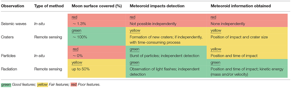
Table 1. Trade-off analysis of methods for the lunar meteoroid impacts observation.
1.3. Lunar Meteoroid Impact Flashes
Light flashes at the Moon are typically observed by detecting a local spike of the luminous energy in the visible spectrum when pointing a telescope at the lunar nightside. The background noise is mainly composed by the Earthshine (Earth reflected light on the Moon surface) in the visible spectrum, and by thermal emissions of the Moon surface in the infrared spectrum (Bouley et al., 2012). Measurements with high signal-to-noise ratios can be obtained through observations of the lunar nightside (Bellot Rubio et al., 2000). The detected luminous energy spike is quantified using the apparent magnitude of the light flash.
Lunar impact flashes detected from Earth-based observations have apparent magnitude between +5 and +10.5 (Oberst et al., 2012), which correspond to very faint signals. Also, Earth-based observations of lunar impact flashes are restricted to periods when the lunar nearside illumination is 10–50% (Ortiz et al., 2006; Suggs et al., 2008). The upper limit restriction is due to the dayside of the Moon glaring the telescope field of view (FOV). The lower limit restriction of 10% corresponds to the New Moon phase. During this phase, the observations should be made when the Moon presents itself at low elevations in the sky (morning or evening), but the observation periods are too short to be useful (Suggs et al., 2008; Oberst et al., 2012).
The first unambiguous lunar meteoroid impact flashes were detected during 1999's Leonid meteoroid showers and were reported in Ortiz et al. (2000). The first redundant detection of sporadic impacts was only reported 6 years later in Ortiz et al. (2006). These events gave origin to several monitoring programs. In 2006, a lunar meteoroid impact flashes observation programme was initiated at NASA Marshall Space Flight Center (Suggs et al., 2008). This facility is able to monitor 4.5 × 10⁶ km2 of the lunar surface, approximately 10 nights per month, subject to weather conditions. Approximately half of the impact flashes observations occur between the Last Quarter and New Moon (0.5–0.1 illumination fraction) and the other half between New Moon and First Quarter (0.1–0.5 illumination fraction). The former monitoring period occurs in the morning (waning phase) and the latter occurs in the evening (waxing phase), covering the nearside part of the eastern and western lunar hemisphere, respectively. 126 high-quality flashes were reported in Suggs et al. (2014), for 266.88 h of monitoring, over a 5 years period. The magnitude range detected is between +10.42 and +5.07, which is estimated to correspond to an impactor kinetic energy range between 6.7 × 10⁻⁷ and 9.2 × 10⁻⁴ kton TNT, taking into account the correction factor of 4 suggested in Ortiz et al. (2015). The corresponding impact velocities range from 24 km/s to 70 km/s.
The most recent monitoring program, NELIOTA, was initiated on February 2017 in Greece under ESA fundings. As of November 2017, 16 validated impacts have been detected over 35 h of observations. NELIOTA aims to detect flashes as faint as +12 apparent visual magnitude (Bonanos et al., 2015) and is the first allowing the determination of the impact flash blackbody temperature by observing both in the visible and infrared spectrum. Monitoring the Moon for impact flashes inherently imposes several restrictions that can be avoided if the same investigation were conducted with space-based assets, such as LUMIO.
1.4. The LUMIO Mission
Observing lunar impacts with space-based assets yields a number of benefits over ground-based ones:
• No atmosphere. Ground-based observations are biased by the atmosphere that reduces the light flash intensity depending upon present conditions, which change in time. This requires frequent recalibration of the telescope. Inherent benefits of the absence of atmosphere in space-based observations are 2-fold: (1) there is no need of recalibrating the instrument, and (2) fainter flashes can be detected.
• No weather. Ground-based observations require good weather conditions, the lack of which may significantly reduce the observation time within the available window. There is no such constraint in space-based observations.
• No day/night. Ground-based observations may only be performed during Earth night, significantly reducing the observation period within the available window. There is no such limitation when space-based observations are performed.
• Full disk. Ground-based observations are performed in the first and third quarter, when nearside illumination is 10–50%. Full-disk observations during New Moon are not possible because of low elevation of the Moon and daylight. Space-based observations of the lunar farside can capture the whole lunar full-disk at once, thus considerably increasing the monitored area.
• All longitudes. Ground-based observations happening during the first and third quarter prevent resolving the meteoroid flux across the central meridian. There is no such restriction in space-based, full-disk observations.
Moreover, observing the lunar farside with space-based assets yields further benefits, i.e.,
• No Earthshine. By definition, there is no Earthshine when observing the lunar farside. This potentially yields a lower background noise, thus enabling the detection of fainter signals, not resolvable from ground.
• Complementarity. Space-based observations of the lunar farside complement ground-based ones
- In space. The two opposite faces of the Moon are monitored when the Moon is in different locations along its orbit;
- In time. Space-based observations are performed in periods when ground-based ones are not possible, and vice-versa.
High-quality scientific products can be achieved with space-based observations of the lunar farside. These may complement those achievable with ground-based ones to perform a comprehensive survey of the meteoroid flux in the Earth–Moon system. All of the above considerations drove the formulation of the LUMIO mission statement:
LUMIO is a CubeSat mission orbiting in the Earth–Moon region that shall observe, quantify, and characterize meteoroid impacts on the lunar farside by detecting their impact flashes, complementing Earth-based observations of the lunar nearside, to provide global information on the lunar meteoroid environment and contribute to Lunar Situational Awareness.
LUMIO mission is conceived to address the following issues.
• Science Question. What are the spatial and temporal characteristics of meteoroids impacting the lunar surface?
• Science Goal. Advance the understanding of how meteoroids evolve in the cislunar space by observing the flashes produced by their impacts with the lunar surface.
• Science Objective. Characterize the flux of meteoroids impacting the lunar surface.
The mission utilizes a 12U form-factor CubeSat which carries the LUMIO-Cam, an optical instrument capable of detecting light flashes in the visible spectrum to continuously monitor and process the data. The mission implements a novel orbit design and latest CubeSat technologies to serve as a pioneer in demonstrating how CubeSats can become a viable tool for deep space science and exploration.
The selection of the operative orbit is detailed throughout the rest of the paper, which is organized as follows. In section 2 the methodology is given, including the criteria defined and the models developed to support the trade-off. In section 3, the trade-off process is detailed by following a hierarchical structure ranging from qualitative to quantitative arguments. Potential operative orbits are presented in section 3.3.4, and final remarks are drawn in section 4.
2. Methodology
The methodology used for LUMIO orbit design relies on the following approach (refer to Figure 1):
1. Evaluation criteria are defined, based on requirements and mission objectives.
2. The relevant orbit types for lunar remote sensing are identified.
3. A preliminary trade-off scans orbit families, accounting for their main characteristics and eliminating clearly non-feasible options. The orbit families encompass two-body Keplerian orbits and several three-body libration point orbits (LPOs). Candidate orbits are the output of the preliminary trade-off.
4. A coverage analysis is performed for the candidate orbits. The physics of the impact is modeled together with the space environment, the local orbital geometry, and the payload characteristics. The model is then validated against a known dataset. Ad-hoc simulations engage the scientific goal of maximizing the number of observable impacts with the need to have lunar full-disk visibility for autonomous optical navigation (Topputo et al., 2017). Non-feasible candidate orbits, according to these criteria, are eliminated and the remaining feasible orbits move on to the next orbital trade-off level.
5. A detailed trade-off quantifies and compares station-keeping and transfer costs for each feasible orbit. Evaluation criteria related to Δv budget are first determined by optimizing the transfer trajectory and station-keeping costs and later applied to select LUMIO operative orbit.
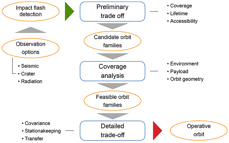
Figure 1. Trade-off scheme for the selection of LUMIO operative orbit.
2.1. Evaluation Criteria for LUMIO Orbits
The evaluation criteria are divided into acceptance criteria and selection criteria. The former are defined based on the science and mission requirements (Topputo et al., 2017). The latter are defined based on orbital performance parameters and allow the selection of optimal orbits, from a set of candidate orbits that meet the acceptance criteria. The acceptance criteria are defined as follows:
EC.A.01 The operational orbit shall allow the detection of meteoroids in the equivalent kinetic energy range at Earth of 10−6 to 10−1 kton TNT.
EC.A.02 The operational orbit shall allow the detection of at least 240 meteoroid impacts during the mission lifetime.
EC.A.03 The operational orbit shall allow the detection of at least 2 meteoroid impacts in the equivalent kinetic energy range at Earth of 10−4 to 10−1 kton TNT.
EC.A.04 The operational orbit shall allow the detection of at least 100 meteoroid impacts in the equivalent kinetic energy range at Earth of 10−6 to 10−4 kton TNT.
EC.A.05 The operational orbit shall allow monitoring of the lunar farside at night.
EC.A.06 The operational orbit shall support a minimum mission lifetime of 1 year, with a maximum total Δv budget of 200 m/s.
EC.A.07 The operational orbit shall be accessible from the departure orbit, with a maximum total Δv budget of 200 m/s.
Evaluation criterion EC.A.01 defines a kinetic energy range to be observed, which is mainly a function of orbit altitude (see section 2.2.2). On the other hand, evaluation criteria EC.A.02–04 are mainly a function of cumulative observation time in the mentioned kinetic energy ranges. In EC.A.02, the approximate number of meteoroid impact flashes used by Suggs et al. (2014) to estimate the lunar impact flux in this range has been considered reasonable for an acceptance criteria. Evaluation criteria EC.A.05 is directly related to the mission requirement of detecting impact flashes on the lunar farside and the need to monitor it at night follows from the fact that impact flashes can only be detected under very low illumination conditions. Finally, in EC.A.06 and EC.A.07, a total Δv budget of 200 m/s is considered based on the constraint on the maximum mass of 24 kg for LUMIO. The allocated Δv budget is deemed reasonable for a CubeSat, in order to support a minimum mission lifetime of 1 year and deployment from a Lunar Orbiter, which would release LUMIO in a given injection orbit around the Moon (see section 3.3).
The selection criteria defined are the following:
EC.S.01 The total number of meteoroids detected during the mission lifetime shall be maximized.
EC.S.02 The total Δv budget shall be minimized.
EC.S.03 The duration spent in observing the lunar full-disk shall be maximized.
The selection criteria are defined in view of mission objectives. As such, in order to determine a good orbit to improve current Earth-based lunar impact flashes observation, the selection criteria are defined in view of the performance of the orbit. EC.S.01 is chosen because one of the main goals of lunar impact flashes monitoring is to improve the current solar system meteoroid models, and a larger number of observations can contribute toward this goal. Moreover, selecting the orbit with the minimum Δv budget can also contribute toward the same goal. This is because the station-keeping Δv could be increased, allowing for a larger mission lifetime and, so, the possibility of detecting more meteoroid impact flashes. Finally, in order to perform reliable optical navigation using the lunar full-disk, EC.S.03 is defined to ensure navigation images can be acquired whenever necessary (Franzese et al., 2018). Furthermore, EC.S.03 also allows for a more uniform coverage of the lunar farside, which can contribute to the understanding of lunar meteoroid impact flux asymmetries.
2.2. Models
2.2.1. Orbital Geometry in Near-Lunar Space
Three different classes of orbits are considered: Keplerian; perturbed Keplerian, and libration point orbits. Only orbits that allow a periodic or repetitive motion with respect to the Moon surface are considered as lunar remote sensing orbits. Orbits whose range to the lunar surface exceeds one third of the Earth–Moon distance (≈ 100, 000 km) are excluded from the analysis. The considered Keplerian orbits are low lunar orbits (LLO) and elliptical lunar orbits (ELO). LLO have a constant low altitude, h, with respect to the Moon surface and a short period (roughly 2 h for the h = 100 km case). For h>100 km, Earth gravitational field affects the satellite motion in such a way that the orbit can no longer be considered as only under the influence of the lunar gravity field (Abad et al., 2009; Carvalho et al., 2010). ELO typically have low perilune altitude and relatively large apolune altitude. Therefore, the spacecraft-to-Moon distance varies significantly in one orbital revolution, along with the coverage periods of certain lunar regions.
The considered perturbed Keplerian orbits are frozen orbits (FO) and Sun-synchronous orbits (SSO). FO are orbits whose orbital elements are stationary, due to reduced or null secular and long-period perturbations. They usually exist only for certain combinations of a (semi-major axis), e (eccentricity), i (inclination), and ω (argument of perilune). The latter is typically fixed at 90 or 270 degrees, meaning that the periapsis of the orbit remains directly above the north or south pole of the central body in case of polar orbits. Hence, the satellite altitude remains constant over each latitude, making coverage patterns repetitive. Two different types of lunar frozen orbits are considered. The first takes only into account perturbations by the zonal terms of the lunar nonspherical gravity field, i.e., Jn-terms, and has low altitudes, i.e., h ≤ 100 km. The second takes also into account perturbations of the Earth gravity field, and has higher altitudes (h>100 km). On the other hand, SSO are orbits whose line of nodes rotates to freeze the orbital plane orientation relative to the Sun, i.e., the orbital plane rotates at ≈0.9856 deg/day as the Earth–Moon system revolves about the Sun. Table 2 summarizes the main characteristics of Keplerian and perturbed Keplerian orbits.
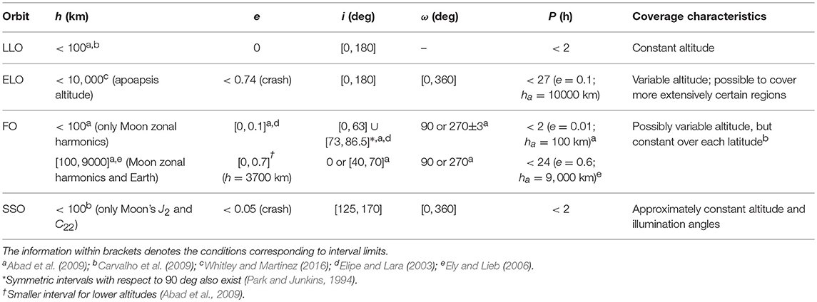
Table 2. Characteristics of Keplerian and perturbed Keplerian lunar remote sensing orbits.
When compared with selenocentric Keplerian orbits, libration point orbits are typically more easily accessible from Earth, have more favorable thermal environments, few or no lunar eclipses, and infrequent Earth shadowing/occultation (Pergola and Alessi, 2012; Whitley and Martinez, 2016). However, they are mostly associated to large instability indicators. The definition of stability index S used in the present work is that of Folta et al. (2015):
where ν denotes the (reciprocal) pair of eigenvalues associated with the stable/unstable subspace of the orbit. With this definition, S>1 indicates instability of the orbit, and S ≤ 1 indicates stability. A large stability index is usually associated with large station-keeping costs, but lower transfer costs (Grebow, 2006). Five types of three-body periodic orbits have been considered for orbital design: Lyapunov orbits (LYO), halo orbits (HO), Lyapunov vertical orbits (VO), distant retrograde orbits (DRO), and low prograde orbits (LoPO). Table 3 summarizes the main characteristics of the LPO, also presented in Figure 2.
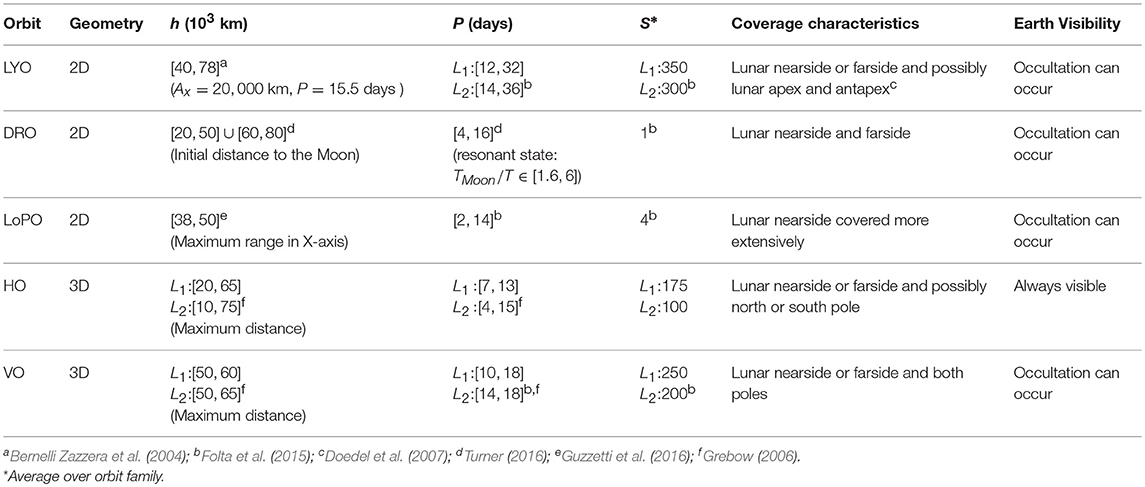
Table 3. Characteristics of libration point lunar remote sensing orbits.
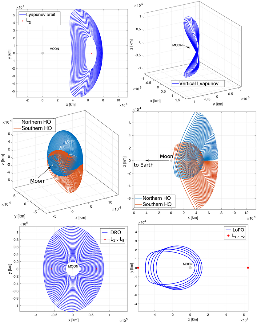
Figure 2. Libration point orbit families, represented in the Moon-centered CRTBP reference frame.
LYO circulate L1, 2 in the circular restricted three-body problem (CRTBP) xy plane and are typically characterized by the amplitude along the x axis (Ax). Their orbital periods in the Earth–Moon system range from approximately 15–30 days and their stability index is relatively high (S~300). HO circulate L1, 2 with a three-dimensional motion. The frequency of their out-of-plane motion matches the in-plane motion and only exist for a specific set of Ay (Farquhar and Kamel, 1973). Halo orbits at the Earth–Moon L1, 2 become almost rectilinear when close to the Moon (Breakwell and Brown, 1979), generating the family of near-rectilinear halo orbits (NRHO), whose stability index is smaller than that of the nominal halos. NRHO are not considered in this work. VO circulate L1, 2 in eight-shaped trajectories, crossing the x axis twice in one orbital period (Folta et al., 2015). Their orbital periods in the Earth–Moon system range from approximately 10–20 days and their stability index is in between that of halo and Lyapunov orbits (S~200). Given their shape, these orbits can be used to monitor both lunar poles in one orbital revolution. DRO circulate the smaller primary (e.g., the Moon) in a retrograde motion (Hénon, 1970). These orbits have no apparent size limit, so they can even encompass both L1 and L2 (Ming and Shijie, 2009). LoPO circulate also the smaller primary, but in a prograde motion (Hénon, 1970). Their orbital periods range from approximately 2–14 days and their stability index vary significantly with size. LoPO may be used to cover more extensively the nearside of the Moon.
2.2.2. Environment Model
In support to the coverage analysis, a meteoroid environment model is needed capable of 1) estimating the kinetic energy of the impactor from the light flash intensity detectable by the payload and of 2) representing the lunar impact time and space flux with accuracy. This model is then used to predict the number of meteoroid impacts that can be observed from a given orbit. Two different methods are used to estimate the detectable kinetic energy. These are referred to as the luminous efficiency method and the blackbody method. The first assumes a directly proportional relation between light emitted in the visible spectrum and the impactor kinetic energy. The second assumes that the impact flash emits radiation as a blackbody and the emitting surface scales with the size of the impact crater.
The luminous efficiency method used consists of the following steps.
1. Estimation of received energy flux (J/m2) in the visible spectrum (Raab, 2002),
where simpact is a number in the range of signals detectable by one pixel of the camera, in e−/pixel (see section 2.2.3 for more details), and are the mean quantum efficiency and mean photon energy over the sensor observation spectrum, respectively, Alens is the area of the optic lens, and τ is a constant that accounts for lens transmissivity, transparency, and the light spreading across multiple pixels.
2. Estimation of the total emitted energy in the visible spectrum (Bellot Rubio et al., 2000),
where d is the distance between the payload sensor and the impact flash and radiation is assumed to be emitted into 2π steradians, as done in Suggs et al. (2014).
3. Estimation of the meteoroid kinetic energy (Bellot Rubio et al., 2000),
where η is the luminous efficiency in the visible spectrum.
The luminous efficiency is assumed to be in the range η∈[5, 50] × 10−4 (Bouley et al., 2012) and its nominal value is assumed to be η = 20 × 10−4 (Ortiz et al., 2015).
The blackbody method used consists of the following steps.
1. Estimation of the flux of electrons (e−/m2) generated in the sensor (Raab, 2002),
2. Estimation of the total flux of photons emitted in the visible spectrum, converted to an electron flux (Bouley et al., 2012),
with
where Δt is the assumed duration of the impact, λ∈[λ1, λ2] is the observed wavelength, and TF is the assumed (constant) blackbody temperature of the flash. L(λ, TF) is Plank's law in W/m2/nm and Eγ(λ) is the energy of a photon (γ).
3. Estimation of the emitting surface area, i.e., the effective area of the impact flash (Bouley et al., 2012):
4. Estimation of the impact's crater diameter,
where ncrater is the ratio between the diameter of the impact flash and respective crater (Bouley et al., 2012). Assuming that the impact is only detected by one pixel, D should be smaller than the ground sampling distance (GSD).
5. Estimation of the meteoroid kinetic energy, from Gault's crater law (Bouley et al., 2012; Madiedo et al., 2015),
where ρp and ρt are the projectile and target densities, g is the gravitational acceleration at the Moon, and θi is the impact angle with respect to the horizontal.
The nominal parameters assume Δt = 10 ms, which is the lower bound of the impact flashes detected on Earth (Bouley et al., 2012), TF = 2, 700 K, which is within the interval mentioned in Suggs et al. (2017), ncrater = 1, which is the minimum ratio assumed in Bouley et al. (2012), ρp = 2000 kg/m3; ρt = 3000 kg/m3 and θi = 45 deg (Bouley et al., 2012). It should be noted that Δt, TM, and ncrater are assumed as constants and not a function of the impactor kinetic energy, as no relation is known yet.
In both methods, for (perturbed) Keplerian orbits the distance between the impact flash and payload is assumed equal to the satellite altitude, i.e., the impact is assumed to occur at nadir. However, such assumption significantly affects the libration point orbits results. The number of impacts detectable closer to the edge of the payload FOV area is found to be approximately 90% lower than the number of impacts detectable at nadir. As such, the impacts are conservatively assumed to occur at the midpoint between nadir and the edge of the FOV-area.
The meteoroid impact flux model used in this work is that of Brown et al. (2002):
where fE is the cumulative number of meteoroid impacts with Earth, per year, for kinetic energies equal or >KEE. However, the meteoroid impact flux at the Moon is smaller than the meteoroid impact flux at Earth given by Equation 11, due to (1) the smaller surface area and (2) the weaker gravity field. As such, in order to scale down the flux at Earth to a meteoroid flux at the Moon, the Moon–Earth surface area ratio and a gravitational correction term for the Earth are taken into account. The gravitational correction term for the Moon is considered negligible (Bouley et al., 2012). The implemented gravitational correction considers both a larger effective target area of Earth and a larger impactor velocity relative to the Earth when compared to true physical values. The gravitational correction factors applied are (Suggs et al., 2014)
where Aeff is the effective cross sectional area of the target body, Aphy is the physical cross sectional area of the target body, vesc is the escape velocity at the target body, and v is the impactor velocity, relative to the target body, before gravitational correction. Assuming vesc = 11 km/s (Suggs et al., 2014) and v = 17 km/s (Bouley et al., 2012), the gravitational correction factors are farea = fKE = 1.42. The cumulative yearly meteoroid impact flux at the Moon is then:
where KEM is the impactor kinetic energy at the Moon and RM and RE are the radii of the Moon and Earth, respectively. For a given instrument FOV, the estimated impact rate detectable (impacts/year), as a function of time, is computed:
where FOVeff(t) is the observable nonilluminated Moon surface area, and KEmin(t), KEmax(t) are the minimum and maximum kinetic energy detectable, estimated using Equations (4–10). Equation 14 also includes a factor of 50% reduction of meteoroid impacts detectable to take into account possible occultations by lunar mountains (Koschny and McAuliffe, 2009). It should be noted that, using Brown's flux in this fashion, it is inherently assumed that the impact flux of meteoroids is uniform across the lunar surface and is evenly distributed throughout the year.
This meteoroid environment model is validated with data from the NELIOTA program: a telescope with 1.2 m diameter, capable of performing observations in the R-band (λ∈[520, 796] nm). Since 16 impacts in 35 h observation time had been detected by November 2017, it is assumed that the program typically detects 0.46 impacts per hour. The visual magnitudes ranged from +11 to +6. Assuming that these values correspond to the limiting capacity of the detector, it is possible to estimate the minimum and maximum signal received at the detector. Then, it is possible to apply both kinetic energy estimation methods and predict the total number of impacts detectable from Earth (d = 384, 401 km). For that purpose, the FOV-area of the telescope has been assumed as 1/3 of the entire (dark) Moon disk. Using the luminous efficiency method, a rate of between 0.35 and 0.12 impacts per hour is determined, assuming Δt∈[10, 33] ms. Using the blackbody method, a rate of 0.13 impacts per hour is estimated. As such, the results obtained with both methods used in this work are the same order of magnitude as the detected in the NELIOTA program.
2.2.3. Payload Model
In order to determine if the signal of an impact flash is detectable by LUMIO's CCD sensor, the concept of signal-to-noise ratio (SNR) is used. Given the signal of the impact (simpact) and the Poisson noise associated with all signals (σ), the SNR is defined as:
where simpact is measured in electrons generated in the CCD, per pixel (e−/pixel), and σ is measured in electrons root-mean-square (rms). The Poisson noise of a signal is defined as and the total Poisson noise is given by
The CCD sensor also has the possibility of amplifying the incoming signals by a gain factor G, at the expense of an excess-noise factor (ENF). When computing the SNR, all signals generated in the detector before the multiplication register must be multiplied by G and the corresponding noises by ENF, as follows:
where , for the first four noise sources considered, which correspond to the incoming signals. In Equation (17), the noise sources that are taken into account are:
• σimpact, the noise associated with the impact flash signal itself.
• σM, the Moon surface background noise, estimated at
whereeRM is the flux of photons received, due to the Moon background light emission, converted to an electron flux Bouley et al. (2012),
and h is the satellite's altitude, TM≈150 K is the assumed (constant) blackbody temperature of the Moon, texp is the exposure time of the sensor and SMoon is the emitting surface of the Moon, which is assumed equal to the Moon surface area observed by one pixel at nadir.
• σC, the cosmic background noise, estimated as follows (Raab, 2002),
wherepRC is the flux of photons received at the sensor,
and it is assumed that the cosmic background noise corresponds to visual magnitude mV = +18, so, 2748 γ/s/m2 per square arc second are received by the sensor (Raab, 2002). AIFOV is the sensor instantaneous FOV in square arc seconds.
• σDC, the CCD internal noise, known as Dark-Current, estimated as follows:
where DC is the number of electrons generated in the sensor per second and per pixel, at a certain temperature.
• σRON, the CCD Read-Out Noise, given in Table 4.
• σOCN, the CCD Off-Chip Noise, estimated as
where offn denotes the off-chip noise, OAR denotes the Output Amplifier Responsivity of the detector and Npixels denotes the total number of pixels of the sensor.
• σQN, the A/D converter's noise, known as Quantisation Noise, estimated as
where capG is the multiplication register capacity (detector with gain) and Nbits is the A/D converter number of bits.
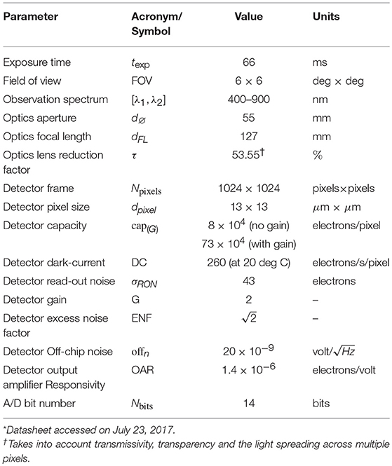
Table 4. LUMIO-Cam parameters, including those of the chosen detector (Teledyne e2V CCD201-20*).
Assuming that the impact flash can be detected for SNR≥SNRmin, the determination of the minimum signal detectable was made by solving Equation (17) for simpact = smin, as
with
On the other hand, the maximum impact flash signal detectable is given by the capacity of the detector (cap), given in Table 4. Given the payload characteristics presented in Table 4 and considering that a signal is detectable for SNRmin = 5, the range of signals detectable by the CCD is given by s = [smin, smax] = [292, 80000] e−/pixel. These values apply for all altitudes, as σM(d) is found to be negligible with respect to other noise sources, and are then used to estimate the minimum and maximum kinetic energy detectable by the payload, using the methods presented in section 2.2.2.
3. LUMIO Operative Orbit Trade-Off
3.1. Preliminary Analysis
The main characteristics of the candidate orbit types presented in section 2 are assessed and compared in order to eliminate non-feasible options by means of criteria EC.A.05-07 and EC.S.01-02 (see section 2.1). Results are presented in Tables 5, 6 for the (perturtbed) Keplerian and three-body orbits, respectively. The first column of the tables indicate the orbit family. The remaining five columns indicate the compatibility of the orbit family with criteria EC.A.05-07 and EC.S.01-02.
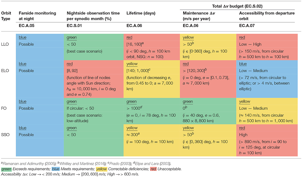
Table 5. Trade-off of (perturbed) Keplerian orbits.
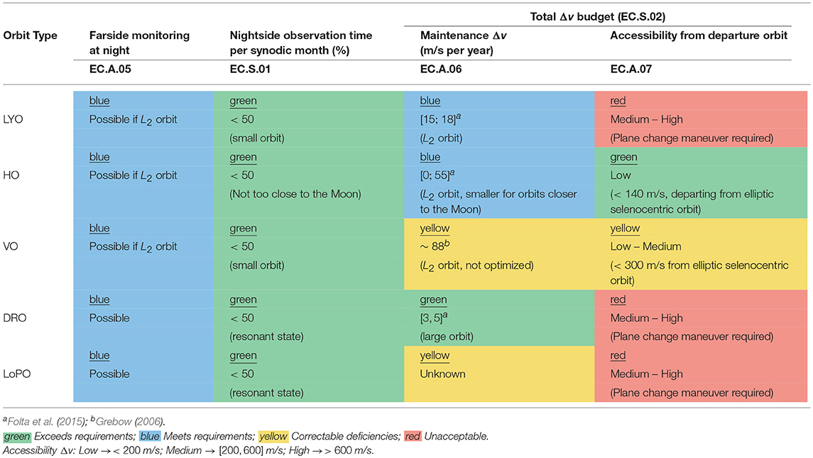
Table 6. Trade-off of CRTBP orbits.
All orbital families presented in section 2, with the exception of L1-circulating LYO, halos, and VO, have orbits which allow the monitoring of the lunar farside at night (EC.A.05), at least once per synodic month.
Selection criteria EC.S.01 requires the maximization of the total number of impacts detected, for which detailed modeling is required. However, it is possible to directly relate this criterion with the total lunar nightside observation time, per synodic month. This is easier to estimate than the total number of meteoroid detections. Recurring to orbital dynamics, it is thus used to assess preliminary performance with respect to EC.S.01. L2-circulating orbits (i.e., LYO, halos, and vertical orbits) observe mostly the lunar farside and opposite lunar phases than an observer on Earth. As such, assuming that < 50% illumination is required for impact flashes detection, these orbits can only observe 50% of the time the lunar nightside, per synodic month. Selenocentric orbits can observe both the lunar nearside and farside. However, for a resonant DRO, the sequence of lunar phases observed by the spacecraft can be very similar to those of L2 orbits. It is conservatevely estimated a lunar nightside observation time of approximately 50%, per synodic month. An analogous reasoning is made for the remaining selenocentric orbits.
The orbital lifetime (EC.A.06) is dominated by the satellite duration before crashing on the Moon or escaping without means of recovery. It is only defined for (perturbed) Keplerian orbits. Since a mission lifetime larger than 1 year is required, this characteristic can be useful in assessing if that requirement is met. Nonetheless, if the natural lifetime of an orbit is smaller than 1 year, it is its maintenance Δv that determines the compliance with EC.A.06. LLO typically have an orbital lifetime smaller than 200 days, the exception being inclinations for which the orbit is frozen (Ramanan and Adimurthy, 2005). SSO orbital lifetime is rouglhy 300 days. On the other hand, the lifetime of ELO varies from 140 days, for e = 0.45, to 1, 000 days, for e = 0.01 (Prado, 2003). A lifetime larger than 1 year is only possible for a low-eccentricity orbit of e < 0.15. Lastly, FO have been estimated to last more than 3 years (Elipe and Lara, 2003).
However, it is mainly the maintenance Δv that dictates compliance with EC.A.06, the exception being frozen orbits that have orbital lifetimes larger than 1 year and, theoretically, do not need intervention (Whitley and Martinez, 2016). There are some ELO and SSO with low eccentricities which also have longer-than-1-year orbital lifetimes, but their coverage characteristics quickly degenerate with time. For highly elliptic ELO, the station-keeping Δv can be larger than 300 m/s, while for SSO and LLO (h = 100 km) it may overcome 50 m/s per year (Whitley and Martinez, 2016). For low-eccentricity orbits, an estimation is done at 120 m/s per year. The maintenance Δv budget for most of the CRTBP orbits has been taken from (Folta et al., 2015). These were computed with a long-term strategy of 12 orbital revolutions as nominal guidance, including random errors in position, velocity and impulsive correction maneuvers, for an average of 500 trials. VO require 88 m/s station-keeping (S/K) Δv per year (Grebow, 2006). No information regarding LoPO maintenance is available.
The accessibility from the departure orbit (EC.A.07) is measured in terms of the Δv spent for the transfer to the operational orbit. For Keplerian orbits, the optimal transfer Δv can easily be estimated resorting the orbital dynamics knowledge of the two-body dynamics. For three-body orbits, the optimal transfer Δv needs to be computed numerically, e.g., using optimization methods. As such, in this preliminary trade-off, only optimal transfers between Keplerian orbits are computed. For three-body orbits, representative values found in literature are assumed.
The amount of propellant spent in reaching the operational orbit and maintaining it are two quantities that should be assessed together, given that there is only a limit for their sum: the total Δv budget (EC.S.02). This should be < 200 m/s to comply with EC.A.06-07 and should be the smallest possible to comply with EC.S.02.
As a result of the preliminary trade-off analysis, summarized in Tables 5, 6, we consider (1) Circular frozen orbits with h∈[100, 1, 000] km and i∈[50, 90] degrees (which is chosen to reduce plane change cost); (2) L2-circulating halo orbits; and (3) L2-circulating vertical orbits. The trade-off is conducted assuming that the Lunar Orbiter would deploy LUMIO either in a 500 km-altitude circular parking orbit or a 200 by 15, 000 km lunar parking orbit. The inclination of this orbit is assumed to be between 50 and 90 degrees.
These orbits have been modeled in order to perform the following coverage analysis. Preliminary lunar frozen orbits have been found by numerically minimizing the amplitude of the osculating eccentricity, taking into account third body perturbations from Earth and the lunar non-spherical gravity model GL0660B (Konopliv et al., 2013), up to degree and order 7. The initial conditions for Halo and Vertical orbits have been found in the CRTBP, using a time-varying targeting scheme. All orbits have been propagated for one synodic month.
3.2. Coverage Analysis
The evaluation criteria related to lunar meteoroid impacts are applied, and a meteoroid impact flashes coverage analysis is performed. The coverage analysis is characterized by the interaction between three modules:
1. FOV-area module. The surface area that an instrument can observe (FOV-area), at one instant or extended period of time, defines the coverage of the central body. The FOV-area of LUMIO is computed considering the instrument working principles, the LUMIO-Cam characteristics, and the actual curvature of the central body. The payload FOV and the S/C position are the two main inputs of this module. Furthermore, is is assumed that the S/C points toward nadir.
2. Lunar nightside monitoring module. The effective FOV-area is defined as the fraction of the FOV-area that it is not illuminated by the Sun. Since lunar impact flashes can only be detected on the lunar nightside, this module allows the determination of the lunar portion in which meteoroids flashes may be actually detected. The main input is the Sun–Moon–spacecraft angle (β), which determines the illumination conditions of the FOV-area, such that
where fdark(t) = β(t)/180 is the percentile dark lunar portion, with β∈[0, 180] deg. In Equation (27), the effective FOV-area is zero when fdark < 0.5, thus no observations can be performed in this range.
3. Meteoroid environment module. Given the range of signals detectable by the payload at each instant and an altitude profile, this module can independently determine the range of kinetic energies detectable by LUMIO (see section 2), for each candidate orbit. Given also the effective FOV-area, the total number of meteoroids detected in the kinetic energy range [KEmin, KEmax], over the mission lifetime, is determined through (1) Estimation of the impact flux (indicator of impacts per year) visible in the satellite effective FOV-area, as function of time (Equation 14); (2) Estimation of the average impact flux visible in the satellite effective FOV-area, during one synodic month by means of an integral function; and (3) Estimation of the total number of meteoroids detected over the mission lifetime (1 year).
3.2.1. Coverage Trade-Off
Figures 3A,B show the minimum and maximum kinetic energy detectable by the LUMIO-Cam from a frozen orbit, for the luminous efficiency and blackbody methods. Only the inclinations which allow the maximum number of detections, per semi-major axis, are presented for brevity, but the results shown are representative of all inclinations. With both methods, KEmin and KEmax increase with altitude, but they considerably disagree in the kinetic energy ranges detectable for frozen orbits. The luminous efficiency method estimates that KE kton TNT and KE kton TNT, while the blackbody method estimates that KE kton TNT and KE kton TNT.
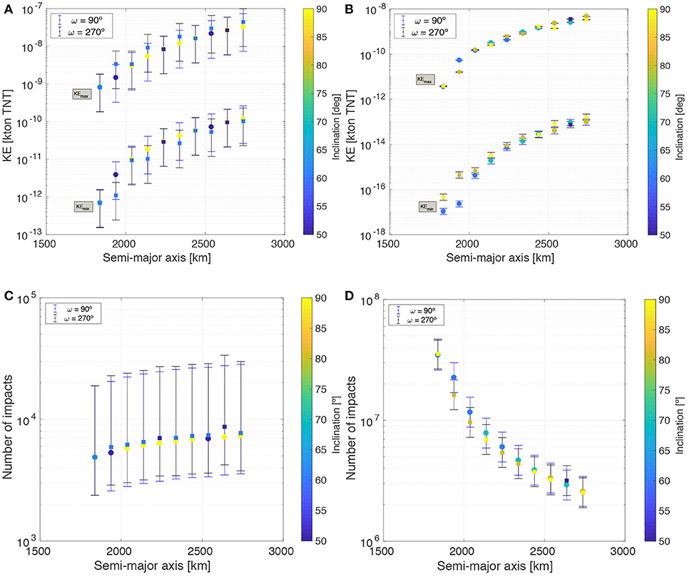
Figure 3. Estimation of detectable kinetic energy range and meteoroid impacts for frozen orbits. (A) Luminous efficiency method. (B) Blackbody method. (C) Detected meteoroids (LE). (D) Detected meteoroids (BB).
Figures 3C,D show the corresponding total number of meteoroid detections during the mission lifetime, where the luminous efficiency method predicts more meteoroid detections for increasing altitude, while the blackbody method predicts the opposite trend. This is because, using the luminous efficiency method the number of impacts detectable is actually proportional to h0.2 and with the blackbody method the number of impacts detectable is proportional to h−1.1, given that, for low altitudes, the FOV-area is proportional to h2 (see section 2.2.2). Furthermore, due to the disagreement in the estimation of KEmin, the luminous efficiency method predicts the detection of much less meteoroids than the blackbody method. The former estimates between 4 and 9 thousands meteoroid detections during the mission lifetime for a frozen orbit, while the later estimates roughly between 2 × 10⁶ and 2 × 10⁸ meteoroids during the same period. Given the LUMIO-Cam optical properties, the estimation made by the luminous efficiency method is more in alignment with the one presented in Oberst et al. (2011). On the other hand, the blackbody method overestimates the number of impacts detectable from a frozen orbit by at least two orders of magnitude.
Figures 4A,B show the minimum and maximum kinetic energy detectable by the LUMIO-Cam for the candidate three-body orbits and for the two kinetic energy estimation methods applied. The black lines represent the kinetic energy requirements as per EC.A.03-04. Being these energies defined at Earth, they are scaled trough the Earth gravitational correction factor (section 2.2.2) to obtain 7 × 10⁻⁷ and 7 × 10⁻² kton TNT at the Moon. The methods disagree with respect to the estimated kinetic energy range, especially regarding KEmax. The blackbody method predicts a wider kinetic energy range, with smaller KEmin and larger KEmax.
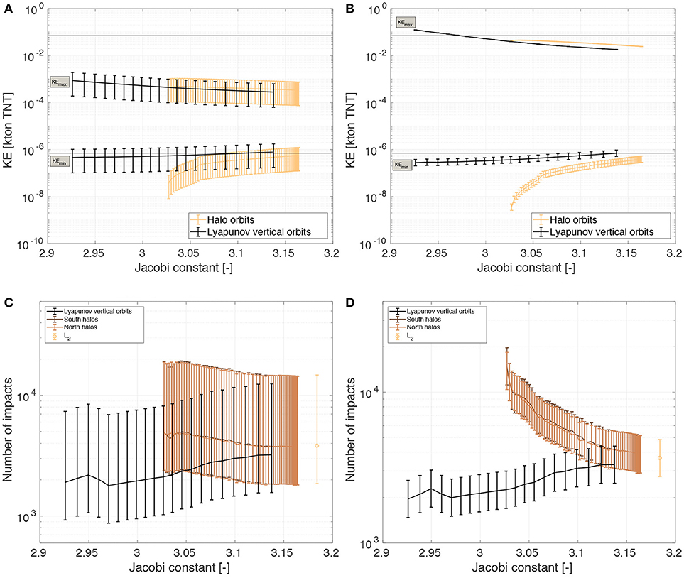
Figure 4. Estimation of detectable kinetic energy range and meteoroid impacts for the considered three-body orbits over the mission lifetime. Black lines represent the kinetic energy limits as set in the requirements (corrected for the Moon). (A) Luminous efficiency method. (B) Blackbody method. (C) Detectable meteoroids (LE). (D) Detectable meteoroids (BB).
The difference between the two methods, for three-body orbits, when it comes to the number of meteoroid detections, is not as prominent as for frozen orbits. Figures 4C,D show the corresponding total number of meteoroid detections during the mission lifetime. As can be seen in this figure, for halos and vertical orbits, the number of impacts estimated by both methods is in the same order of magnitude (between 103 and 104). This is because, for higher altitudes, the methods are in agreement with respect to KEmin, parameter which drives the number of meteoroid detections. The total number of detections estimated for a satellite permanently at the Earth–Moon L2 is also presented, for comparison. The results at L2 represent a limit case for L2-circulating candidate orbits.
The error bars shown here for the luminous efficiency method are associated with the luminous efficiency uncertainty, while the errors bars shown for the blackbody method are a 1σ error related to the magnitude measured by the CCD sensor (Raab, 2002). The blackbody method results show smaller error bars than the luminous efficiency results, but it inherently has more assumptions than the luminous efficiency method and the possible errors associated with those assumptions are not represented in the results shown here.
The results presented here do not account for scattered light from the Moon dayside, consequent detector blooming, and impact flash detection redundancy. In fact, scattered light and blooming may potentially hinder the detection of impact flashes and influence the minimum detected kinetic energy estimation the most, as opposed to the maximum detected kinetic energy. Impact flash detection redundancy can be dealt with in two ways: (1) by slightly defocussing the LUMIO-Cam, in order to avoid false positives; or (2) by adding a second detector to the camera. In both cases, the minimum kinetic energy estimation is also affected. However, to compensate for the loss of signal, the camera sensitivity can be increased with gains G>2. These issues affect neither the assessment of orbit types made in this work nor the validity of the coverage trade-off that follows. These issues will be taken into account in future mission design phases.
The coverage trade-off accounts for evaluation criteria EC.A.01-04. Table 7 displays the orbit trade-off for the results of both luminous efficiency method and blackbody methods, as the two sets of results obtained lead to identical conclusions on orbits feasibility. Both methods exclude frozen orbits (1 out of 4 acceptance criteria related to meteoroid impacts met), while both halo and vertical orbits meet all acceptance criteria. The halo family has the additional advantage of allowing a constant visibility of the spacecraft from Earth and a quasi-resonance 2:1 with the synodic period.
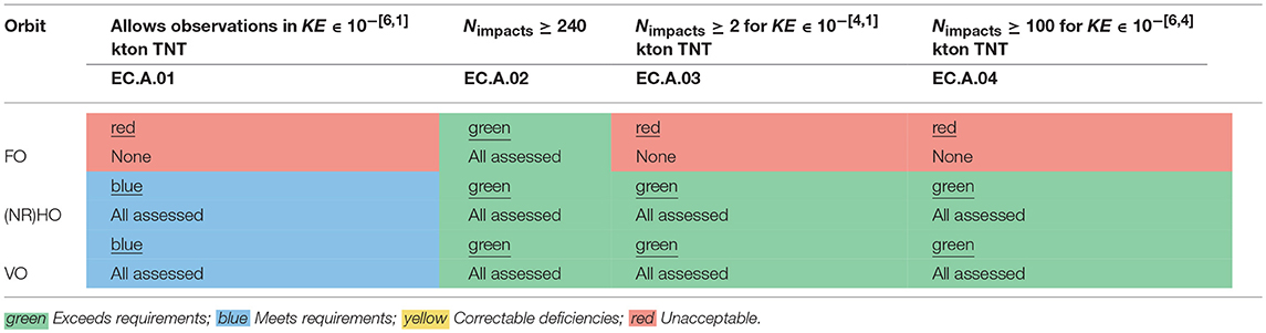
Table 7. First orbit trade-off, given the results of both luminous efficiency method and blackbody method.
3.3. Detailed Analysis
It has been shown that remotely detecting flashes is the only technically and economically viable option for a CubeSat to monitor meteoroid impacts on the lunar surface. When considering the conclusions of the preliminary trade-off (section 3.1), the coverage trade-off (section 3.2), the mission type flight heritage, and solar eclipse occurrences, the Earth–Moon L2 halo family is baselined for LUMIO mission. The vertical Lyapunov orbit family is selected as back-up plan and it is not detailed in this paper.
The LUMIO mission is divided in 4 well defined phases (refer to Figure 5),
1. Parking:
(a) Starts when the lunar orbiter deploys LUMIO on the prescribed selenocentric elliptic parking orbit (orbital elements of the parking orbit are shown in Table 8);
(b) Ends when LUMIO performs the Stable Manifold Injection Maneuver (SMIM);
(c) Lasts 14 days.
2. Transfer:
(a) Starts when LUMIO completes the SMIM;
(b) Ends when LUMIO performs the Halo Injection Maneuver (HIM);
(c) Lasts 14 days.
3. Operative:
(a) Starts when LUMIO completes the HIM;
(b) The primary mission modes during the operative phase are Science Mode and Navigation and Engineering Mode (or Nav&Eng), that alternate between every other orbit;
(c) Ends after 1 year of operations.
4. End of Life (EoL):
(a) Starts with de-commission of all (sub)systems;
(b) Ends when the EoL maneuver is correctly performed for safe disposal of the spacecraft.
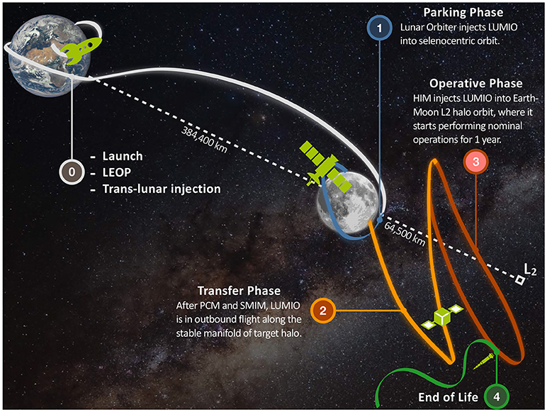
Figure 5. Outline of LUMIO mission phases.

Table 8. Main parameters for the transfer phase.
3.3.1. Earth–Moon L2 Halos in High-Fidelity Model
A set of quasi-periodic halo orbits (sometimes referred here as quasi-halos or quasi-halo orbits) about Earth–Moon L2 are found by employing the methodology described in Dei Tos and Topputo (2017a). Fourteen quasi-halo orbits are computed in the high-fidelity roto-pulsating restricted n-body problem (RPRnBP) and saved as SPICE2 kernels (see Dei Tos and Topputo, 2017a for more details on frames and models). The initial feeds to compute the quasi-halo samples are Earth–Moon three-body halos at 14 different Jacobi constants, ranging from Cj = 3.04 to Cj = 3.1613263. The latter value corresponds to the one assumed for the very first iteration of the activities. All orbits are computed starting from 2020 August 30 00:00:00.000 TDB. Although quasi-halos, shown in Figure 6, are computed for a fixed initial epoch, the persistence of libration point orbits in the solar system ephemeris model allows wide freedom in the refinement algorithm also for mission starting at different epochs (Dei Tos and Topputo, 2017b).
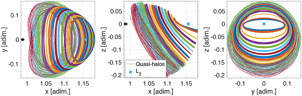
Figure 6. Projection of Earth–Moon L2 quasi-halos in the roto-pulsating frame. (adim. stands for nondimensional variable).
Quasi-halo orbits of Figure 6 are all possible LUMIO operative orbits. As the orbit becomes more energetic (or as its CRTBP Jacobi constant decreases), the quasi-halo exhibits a wider range of motion both in terms of a) Moon range and of b) geometrical flight envelope about the corresponding CRTBP trajectory. The latter trend is disadvantageous when a hard pointing constraint must be respected (e.g., Moon full disk on optical instrument). On the other hand, the lunar distance places a constraint on the minimum FOV for the optical instrument on board LUMIO to be able to resolve the Moon full disk at any location along the quasi-halo, compatibly with evaluation criteria EC.S.03. Bar charts in Figure 7 show the ranges from the lunar surface to the quasi-halo samples. For given values of the camera FOV, simple trigonometric calculations provide the minimum distance above which the Moon disk is entirely seen by the instrument. The wider the FOV, the closer LUMIO can get to the Moon still being able to see its full disk. The horizontal dashed lines in Figure 7 indicate this distance for different values of FOV in degrees.
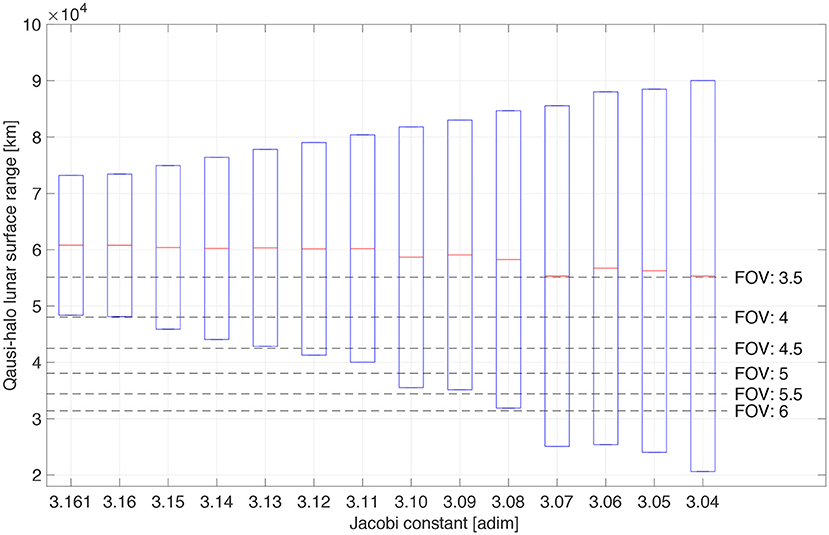
Figure 7. Bars for quasi-halos ranges from lunar surface.
3.3.2. Orbital Transfer
The transfer phase of LUMIO is done entirely in the CRTBP. Free transport mechanisms are leveraged to reach a target halo. Specifically, intersection in the configuration space is sought between the halo stable manifolds and the selenocentric injection orbit in which LUMIO is deployed by the lunar orbiter. Since the sought intersection occurs only in configuration space, a maneuver is necessary for orbital continuity. This maneuver places the spacecraft on the stable manifold of the target halo and is thus called stable manifold injection maneuver (SMIM), ΔvSMIM. The transfer phase starts when the SMIM is executed, and ends after the halo injection maneuver (HIM), ΔvHIM, inserts the S/C into the target halo orbit. The aim of the transfer design analysis is to find the parameters of the injection orbit and the stable manifold that lead to a minimum ΔvSMIM at the intersection. The optimization problem is stated and solved with a NLP method.
It is convenient to briefly recall the methodology used to numerically compute the invariant manifolds in the CRTBP. This approach relies on finding a linear approximation of the manifold in the neighborhood of an orbit. An algorithm is implemented that scans the stable manifold space by varying the time along the originating halo, tpo, and the time along the stable manifold, tsm. Once tpo and tsm are specified, the stable manifold is completely determined (Topputo, 2016). tpo uniquely specifies a state along the halo, x(tpo). At x(tpo), the invariant manifolds are locally spanned by the stable and unstable eigenvectors of M(tpo), the monodromy matrix associated to x(tpo). The initial conditions used to compute the stable manifold are xs0 = x(tpo)±εvs, where vs is the stable eigenvector of M(tpo) and ε is a small displacement perturbing in the stable direction, whereas the ± discriminates which of the two branches of the manifold has to be generated. As for ε, it should be small enough to preserve the local validity of the linear approximation, but also large enough to prevent from long integration times needed to compute the manifold. In this work, ε = 10−6 has been used, consistently with the arguments in Gómez et al. (1993). tsm is the duration xs is flown in backward time. The stable manifold state yields:
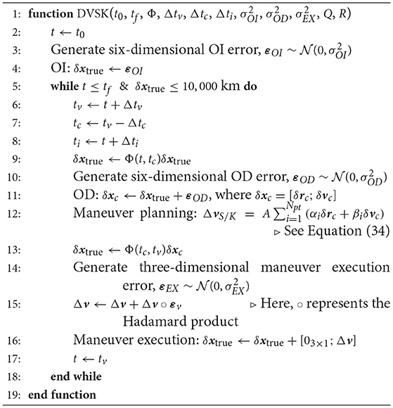
where φ is the flow of the CRTBP from xs0 to −tsm. An outline of the transfer design logic is shown in Algorithm 1. The problem of transfer design with an optimal impulsive maneuver can be formally stated as a constrained minimization:
where
where rt is the position along the injection orbit, and rs is the position along the stable manifold according to Equation (28). The minimization is solved with an active-set algorithm. Algorithm 1 is applied to all halos in the Jacobi energy range detailed above. Note that if the inclination of the injection orbit is found to be outside of the admissible range ([50, 90] deg), a plane chance maneuver (PCM) is added. The transfer parameters to quasi-halo generated by Cj = 3.09 are shown in Table 8. As expected, the SMIM occurs at the periselene of the injection orbit (θ≈0).
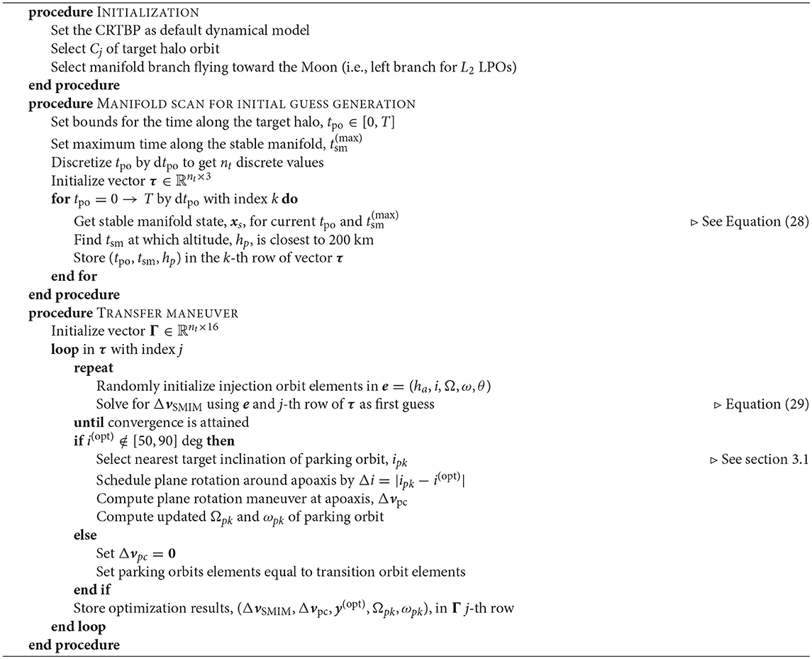
Algorithm 1. Transfer design.
3.3.3. Station-Keeping
In many cases, it is not strictly necessary for the spacecraft to move precisely along the nominal trajectory to accomplish mission objectives. Indeed, once the nominal orbit is determined, it is desired to maintain the spacecraft within some region (e.g., torus- or box-shaped) about the reference path. Non-modeled perturbations and errors will cause the spacecraft to drift from the nominal path, and the unstable nature of the libration point orbits will further amplify the deviation. Assuming discrete and impulsive corrections, the station-keeping problem consists in finding the required corrective maneuvers in terms of magnitude, direction, and timing of each Δv. In optimal station-keeping problems, the total Δv budget is minimized.
In light of the limited Δv capability, fuel consumption for station-keeping (S/K) around the operative orbits will be a critical factor for mission sustainability. Taking advantage of the generated orbits as reference trajectories, a computationally efficient Monte-Carlo routine is devised for estimation of the cost of each S/K maneuver. An effort is directed toward the development of a station-keeping strategy that can be used to maintain CubeSats near such nominal LPOs.
The S/K cost is estimated by employing the target points method (TPM) first introduced in Dwivedi (1975), then adapted to the problem of LPOs by Howell and Pernicka (1993), and finally used for JAXA's EQUULEUS mission analysis (Oguri et al., 2017). A massive Monte-Carlo simulation is performed with 10, 000 samples, considering the impact of the injection, tracking, and maneuver execution processes on the nominal orbit determined in the presence of solar radiation pressure and gravity of the main solar system celestial bodies (i.e., Sun, 8 planets, the Moon, and Pluto). To precisely simulate a realistic trajectory,
1. The initial conditions of the quasi-halos are altered to account for orbit insertion error.
2. Tracking windows are considered in which orbit determination (OD) campaigns modify the actual knowledge of the spacecraft state by means of optical measurements and non-linear filtering. Because of various uncertainties in the OD process, the spacecraft position and velocity are never exactly known. To simulate tracking errors, the six S/C states are altered at the end of each OD campaign.
3. At various times along the trajectory, the S/K strategy will determine that a maneuver is required, and its magnitude and direction will be computed. To model the inaccuracy of maneuvers actual implementation, each ΔvS/K component is randomly altered.
The orbit injection, εOI, orbit determination, εOD, and the maneuver execution, εEX, errors are all modeled and generated with zero-mean Gaussian distributions, i.e., , , , where , , are the covariances of the orbit insertion, orbit determination, and maneuver execution uncertainties, respectively.
The station-keeping maneuvers are conducted at specific selected epochs during the mission. That is, maneuver timings are parameters of the S/K strategy, rather than variables. Referring to Figure 8, every OD campaign is always terminated Δtc time units before the maneuver execution. Δtc is termed cut-off duration and it is necessary to compute, schedule, and prepare the maneuver. The S/K maneuver planning is assumed to use Npt downstream points, i.e., the target points, as reference states to compute the maneuver magnitude and direction. In Figure 8, there are two target points, Npt = 2, and one S/K maneuver per halo orbit. The algorithm for the detailed station-keeping cost analysis is shown in Algorithm 2.
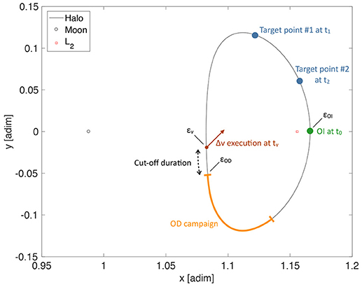
Figure 8. Overview of S/K simulation process and target points method.
Algorithm 2. Cost estimation for of station-keeping along a reference quasi-halo.
The TPM provides optimal ΔvS/K computed as solution of a LQR problem that minimizes a weighted sum of the maneuvers cost and the position deviation from a reference trajectory at Npt downstream control points. The cost function reads
where ΔvS/K is the station-keeping maneuver, Q the cost weight matrix, di the predicted position deviation from the reference trajectory at the i-th target point, and Ri the weighing matrix of the deviation at the i-th target point. The position deviation is predicted by means of the state transition matrix of the reference trajectory, Φ:
In Equation (33), Φrr and Φrv are 3-by-3 matrices that map deviation of position and velocity, respectively, to a position deviation at a subsequent epoch, tc is the cut-off epoch, tv is the maneuver execution epoch, and ti the epoch of the i-th target point. The solution of the minimization problem yields the analytic expression for the optimal station-keeping maneuver:
Table 9 reports the standard deviations of orbit insertion, navigation, and maneuver execution errors for the S/K analysis. The values of Table 9 are in well accordane with existing applications (Folta et al., 2014). More important, simulations have shown the standard deviations of Table 9 can be achieved with the autonomous optical navigation algorithm on-board LUMIO (Franzese et al., 2018). All parameters for the correct functioning of Algorithm 2 have been fine-tuned with extensive simulation campaigns. The parameters fine-tuned values of the S/K algorithm are shown in Table 10. The cut-off duration of 12 h is at the same time sufficiently short to prevent the spacecraft state knowledge from growing excessively, and long enough to schedule maneuver execution operations on-board LUMIO. The target points are located at 35 and 42 days after orbit insertion and any subsequent S/K maneuvers. This ensures approximately 1 month of operations in case of maneuver execution failure. Finally, having the eigenspectrum of Q a larger magnitude than that Ri means the optimization weighs the deviation with respect to reference position more than the ΔvS/K cost.
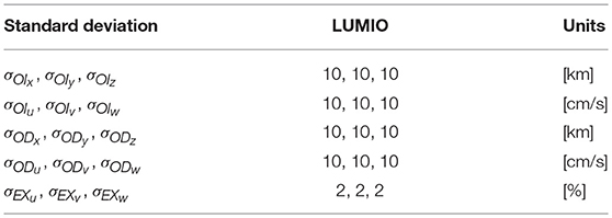
Table 9. Standard deviations.
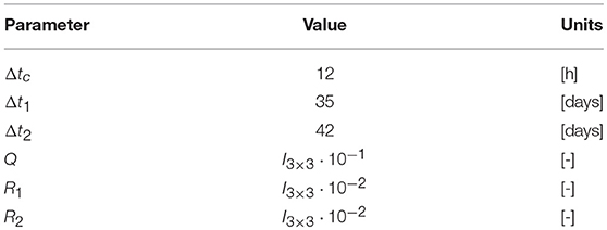
Table 10. Standard deviations.
Figure 9 shows the strategy employed for station-keeping maneuvers timing. For clarity, just 70 days of operations are shown and the quasi-halo orbital period is assumed to be fixed and equal to 14 days. The first quasi-halo orbit is entirely dedicated to recover any orbit insertion (OI) errors by means of two maneuvers, 1 and 7 days after OI, respectively. In the orbits after that, nominal operations occur, i.e., there is a series of Nav&Eng and Science orbits. Three S/K maneuvers are placed within the Nav&Eng orbit: the first at the entry point, the second in the middle (i.e., 7 days after the entry), and the third at the end of the Nav&Eng orbit. This maneuvers frequency configuration allows for pristine Science orbit operations, albeit it increases the cost when compared to a more spread and regular distribution of S/K maneuvers.
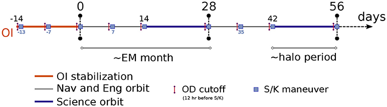
Figure 9. Strategy for station-keeping maneuvers timing.
Station-keeping cost is computed for 1 year of life cycle for each of the quasi-halos considered. To obtain reliable station-keeping cost estimation results, a massive Monte-Carlo simulation of 10, 000 cases is performed with respect to each reference orbit generated. Each Monte-Carlo run employs Algorithm 2 to compute S/K cost for a realization of εOI, εOD, and εEX. Table 11 displays the 1-year S/K cost with 1σ, 2σ, and 3σ confidence. The Monte-Carlo data is fitted by means of an Inverse Gaussian distribution. As expected, the S/K cost increases for smaller (i.e., higher Jacobi constant) quasi-halos. This trend reflects the stability (eigenspectrum of monodromy matrix) properties of halo orbits. That is, a larger halo is generally less unstable and thus cheaper to maintain.
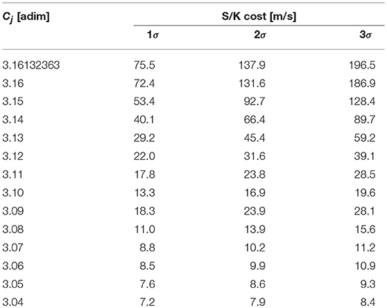
Table 11. Confidence for the 1-year station-keeping cost.
Preliminary observations have been made on alternative station-keeping strategies: an i) Orbit continuation approach and the ii) Floquet unstable modes cancellation method (FM). Although the FM appears as the least expensive in terms of station-keeping total budget (Folta et al., 2014), the TPM is able to give a wider latitude on the selection of the S/K maneuver epoch and phasing, favoring LUMIO orbital geometry and ConOps. Indeed, the FM tends to place S/K maneuvers when the halo unstable component exceeds a defined threshold, regardless of the Phase LUMIO is flying. A further analysis on how to adapt the Floquet modes approach to the LUMIO case may still reduce the station-keeping costs presented in this work. In addition, the ΔvS/K calculation may be overly constrained since the LQR strategy requires the use of target locations and fine-tuning of weight matrices. A different optimization may also reduce the S/K costs presented here.
3.3.4. Detailed Trade-Off
Figure 10 shows the total transfer cost for different halos. The cost includes S/K, SMIM, and plane change maneuvers. It is conjectured the reason why the transfer cost has a clearcut minimum area is 2- fold. (1) For high energy levels (i.e., low Jacobi constant), the stable manifold configuration space does not get close enough to the Moon to permit intersection with the selenocentric transition orbit. At the other end of the spectrum, (2) for high Jacobi constant values, the stable manifolds cross the lunar region sufficiently close to provide patching opportunities with a selenocentric transition orbit, but the speed mismatch is comparatively large. i.e., the outbound stable manifold is much faster than the S/C at periselene.
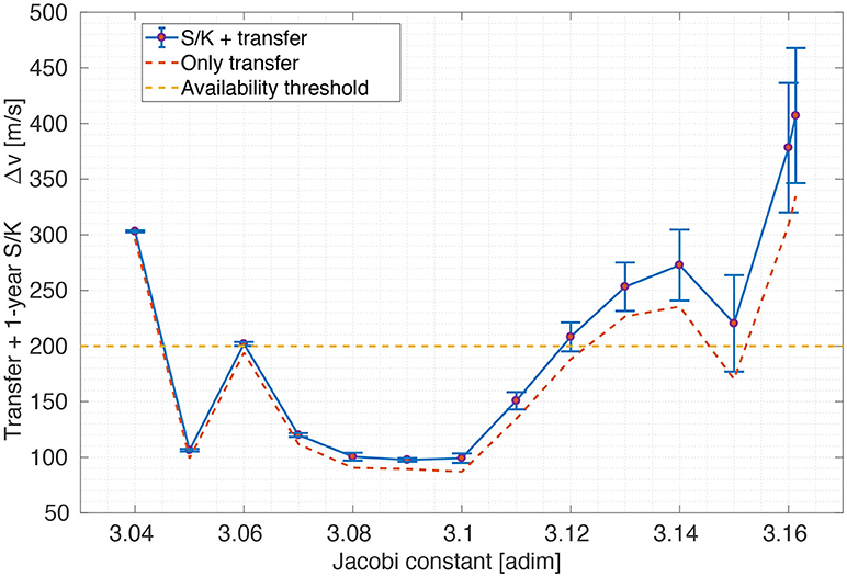
Figure 10. Total transfer cost for different halos.
Quasi-halo generated from Cj = 3.09 is the designated LUMIO operative orbit. The selection of LUMIO operative orbit is based on results of Figure 10. Indeed, the quasi-halo is located at the center of a minimum plateau for total transfer cost which provide both a) Optimality of maneuvers cost, and b) Robustness against errors in the actual energy level of the injected stable manifold.
The selected operative orbit for the LUMIO mission is the most suitable only according to the specified evaluation and acceptance criteria. The selection may change if additional criteria and requirements are investigated in a further step of the mission.
Mission Δv budgets for each maneuver and phase are reported in Table 12 with both deterministic and confidence values. The total 1σ-cost is 154.4 m/s, which is also in line with a 12U CubeSat volume and mass budgets and with acceptance criteria EC.A.06–07. Note that ESA “Margin philosophy for science assessment studies” (Ref. SRE-PA/2011.097/, item MAT-DV-14) states that stochastic maneuvers shall be calculated based on the 3σ confidence interval with no additional margins (SRE-PA and D-TEC staff, 2012). The choice to consider a 1σ confidence interval on stochastic maneuvers for LUMIO is motivated by the inherently higher risk of a low-cost mission. Nonetheless, the overall stochastic Δv computed based on a 95.32% confidence level of a combination of all stochastic maneuvers is smaller than linear sum by 19%. With this approach, the 3σ Δv budget sums up to 191.3 m/s (195.5 m/s with margins on SMIM, HIM, and disposal maneuver), which is still within the bounds for mission feasibility, according to EC.A.06-07.
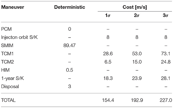
Table 12. Mission Δv budgets for LUMIO operative orbit.
4. Conclusion
The primary science goal of LUMIO mission is to observe meteoroid impact flashes on the lunar farside in order to study the characteristics of meteoroids and to improve the meteoroid models of the solar system. This might lead to a further study of the sources of these meteoroids, such as asteroids in the near-Earth environment and comets. The LUMIO mission complements ground-based observations with remote space-based observations, so improving the lunar situational awareness.
A number of potential orbit families have been considered as candidate operative orbits for LUMIO, namely Keplerian, perturbed-Keplerian, and three-body orbits. An orthodox trade-off logic has been followed with hierarchical structure. An initial pruning has been made based on the way qualitative indicators delivered against acceptance and selection criteria. A second-level trade-off has been performed by coupling the developed models for the environment, impact flash, payload, and astrodynamics. The capability of the payload to resolve the impact flash in each of the candidate orbits as well as to satisfy the mission requirements has been assessed. As a result, L2 halo orbits have been selected. Within the third-level trade-off, a fully quantitative analysis has been conducted by considering the accessibility and station-keeping costs with a high-fidelity concept of operations. Eventually, the LUMIO operative orbit has been baselined.
Author Contributions
All authors listed have made a substantial, direct and intellectual contribution to the work, and approved it for publication.
Funding
The work described in this paper has been funded by the European Space Agency through Contract No. 4000120225/17/NL/GLC/as.
Conflict of Interest Statement
The authors declare that the research was conducted in the absence of any commercial or financial relationships that could be construed as a potential conflict of interest.
Acknowledgments
The work described in this paper is a spin-off of a bigger project, namely the LUMIO Phase 0 design. For this reason the authors are grateful to the rest of LUMIO Team: M. Massari, J. Biggs, S. Ceccherini, K. Mani, V. Franzese, A. Cervone, P. Sundaramoorthy, S. Mestry, S. Speretta, A. Ivanov, D. Labate, A. Jochemsen, Q. Leroy, R. Furfaro, K. Jacquinot, as well as to the Technical Officers at ESA: Roger Walker and Johan Vennekens. The authors are also grateful to Detlef Koschny and Chrysa Avdellidou from ESA NEO Segment for their valuable inputs.
Footnotes
1. ^ https://www.minorplanetcenter.net/. Last retrieved on May 2018.
2. ^ SPICE is NASA's Observation Geometry and Information System for Space Science Missions (Acton Jr, 1996; Acton Jr et al., 2018). The toolkit is freely available through the NASA NAIF website http://naif.jpl.nasa.gov/naif/. Last downloaded on February 7, 2018.
References
Abad, A., Elipe, A., and Tresaco, E. (2009). Analytical model to find frozen orbits for a lunar orbiter. J. Guid. Control Dyn. 32, 888–898. doi: 10.2514/1.38350
Acton Jr, C. (1996). Ancillary data services of nasa's navigation and ancillary information facility. Planet. Space Sci. 44, 65–70. doi: 10.1016/0032-0633(95)00107-7
Acton Jr, C., Bachman, N., Semenov, B., and Wright, E. (2018). A look towards the future in the handling of space science mission geometry. Planet. Space Sci. 150, 9–12. doi: 10.1016/j.pss.2017.02.013
Bellot Rubio, L. R., Ortiz, J. L., and Sada, P. V. (2000). Luminous efficiency in hypervelocity impacts from the 1999 lunar leonids. Astrophys. J. Lett. 542, L65–L68. doi: 10.1086/312914
Bernelli Zazzera, F., F. Topputo, F., and Massari, M. (2004). Assessment of Mission Design Including Utilization of Libration Points and Weak Stability Boundaries. Technical report, Ariadna Study, ESA Contract No. 18147/04/NL/MV.
Bonanos, A., Xilouris, M., Boumis, P., Bellas-Velidis, I., Maroussis, A., Dapergolas, A., et al. (2015). NELIOTA: ESA's new NEO lunar impact monitoring project with the 1.2 m telescope at the National Observatory of Athens. Proc. Int. Astron. Union 10, 327–329. doi: 10.1017/S1743921315006973
Bouley, S., Baratoux, D., Vaubaillon, J., Mocquet, A., Le Feuvre, M., Colas, F., et al. (2012). Power and duration of impact flashes on the moon: implication for the cause of radiation. Icarus 218, 115–124. doi: 10.1016/j.icarus.2011.11.028
Breakwell, J., and Brown, J. (1979). The halo family of 3-dimensional periodic orbits in the earth–moon restricted 3-body problem. Celestial Mech. 20, 389–404. doi: 10.1007/BF01230405
Brown, P. G., Assink, J. D., Astiz, L., Blaauw, R., Boslough, M. B., Borovička, J., et al. (2013). A 500-kiloton airburst over Chelyabinsk and an enhanced hazard from small impactors. Nature 503, 238–241. doi: 10.1038/nature12741
Brown, P. G., Spalding, R. E., ReVelle, D. O., Tagliaferri, E., and Worden, S. P. (2002). The flux of small near-Earth objects colliding with the Earth. Nature 420, 294–296. doi: 10.1038/nature01238
Carvalho, J. P. D. S., De Moraes, R. V., and Prado, A. F. B. A. (2009). Nonsphericity of the moon and near sun-synchronous polar lunar orbits. Math. Probl. Eng. 2009:740460. doi: 10.1155/2009/740460
Carvalho, J. P. D. S., Vilhena de Moraes, R. V., and Prado, A. F. B. A. (2010). Some orbital characteristics of lunar artificial satellites. Celestial Mech. Dyn. Astron. 108, 371–388. doi: 10.1007/s10569-010-9310-6
Ceplecha, Z., Borovička, J., Elford, W. G., ReVelle, D. O., Hawkes, R. L., Porubčan, V., et al. (1998). Meteor Phenomena and Bodies. Space Sci. Rev. 84, 327–471. doi: 10.1023/A:1005069928850
Dei Tos, D. A., and Topputo, F. (2017a). On the advantages of exploiting the hierarchical structure of astrodynamical models. Acta Astronaut. 136, 236–247. doi: 10.1016/j.actaastro.2017.02.025
Dei Tos, D. A., and Topputo, F. (2017b). Trajectory refinement of three-body orbits in the real solar system model. Adv. Space Res. 59, 2117–2132. doi: 10.1016/j.asr.2017.01.039
Doedel, E., Romanov, V., Paffenroth, R., Keller, H., Dichmann, D., Galán-Vioque, J., et al. (2007). Elemental periodic orbits associated with the libration points in the circular restricted 3-body problem. Int. J. Bifurcat. Chaos 17, 2625–2677. doi: 10.1142/S0218127407018671
Dwivedi, N. P. (1975). Deterministic optimal maneuver strategy for multi-target missions. J. Optimization Theory Appl. 17, 133–153. doi: 10.1007/BF00933919
Elipe, A., and Lara, M. (2003). Frozen orbits about the moon. J. Guid. Control Dyn. 26, 238–243. doi: 10.2514/2.5064
Ely, T., and Lieb, E. (2006). Constellations of elliptical inclined lunar orbits providing polar and global coverage. J. Astronaut. Sci. 54, 53–67. doi: 10.1007/BF03256476
Farquhar, R. and Kamel, A. (1973). Quasi-periodic orbits about the translunar libration point. Celestial Mech. 7, 458–473. doi: 10.1007/BF01227511
Folta, D. C., Bosanac, N., Guzzetti, D., and Howell, K. C. (2015). An earth–moon system trajectory design reference catalog. Acta Astronaut. 110, 341–353. doi: 10.1016/j.actaastro.2014.07.037
Folta, D. C., Pavlak, T. A., Haapala, A. F., Howell, K. C., and Woodard, M. A. (2014). Earth–moon libration point orbit stationkeeping: Theory, modeling, and operations. Acta Astronaut. 94, 421–433. doi: 10.1016/j.actaastro.2013.01.022
Franzese, V., Di Lizia, P., and Topputo, F. (2018). “Autonomous optical navigation for lumio mission,” in 2018 Space Flight Mechanics Meeting, AIAA SciTech Forum (Kissimmee, FL: American Institute of Aeronautics and Astronautics), 1–11. doi: 10.2514/6.2018-1977
Gómez, G., Jorba, A., Masdemont, J., and Simó, C. (1993). Study of the transfer from the earth to a halo orbit around the equilibrium point l1. Celestial Mech. Dyn. Astron. 56, 541–562. doi: 10.1007/BF00696185
Grebow, D. (2006). Generating Periodic Orbits in the Circular Restricted Three-Body Problem with Applications to Lunar South Pole Coverage. Master of Science in Aeronautics and Astronautics Thesis, Purdue University.
Gudkova, T. V., Lognonné, P. H., and Gagnepain-Beyneix, J. (2011). Large impacts detected by the Apollo seismometers: impactor mass and source cutoff frequency estimations. Icarus, 211, 1049–1065. doi: 10.1016/j.icarus.2010.10.028
Guzzetti, D., Bosanac, N., Haapala, A. F., Howell, K. C., and Folta, D. C. (2016). Rapid trajectory design in the earth–moon ephemeris system via an interactive catalog of periodic and quasi-periodic orbits. Acta Astronaut. 126, 439–455. doi: 10.1016/j.actaastro.2016.06.029
Howell, K. C., and Pernicka, H. J. (1993). Stationkeeping method for libration point trajectories. J. Guid. Control Dyn. 16, 151–151. doi: 10.2514/3.11440
Konopliv, A. S., Park, R. S., Yuan, D. N., Asmar, S. W., Watkins, M. M., Williams, J. G., et al. (2013). The JPL lunar gravity field to spherical harmonic degree 660 from the GRAIL Primary Mission. J. Geophys. Res. Planets 118, 1415–1434. doi: 10.1002/jgre.20097
Koschny, D., and McAuliffe, J. (2009). Estimating the number of impact flashes visible on the Moon from an orbiting camera. Meteorit. Planet. Sci. 44, 1871–1875. doi: 10.1111/j.1945-5100.2009.tb01996.x
Madiedo, J. M., Ortiz, J. L., Organero, F., Ana-Hernández, L., Fonsenca, F., Morales, N., et al. (2015). Analysis of Moon impact flashes detected during the 2012 and 2013 Perseids. Astron. Astrophys. 577:A118. doi: 10.1051/0004-6361/201525656
Ming, X., and Shijie, X. (2009). Exploration of distant retrograde orbits around moon. Acta Astronaut. 65, 853–860. doi: 10.1016/j.actaastro.2009.03.026
Oberst, J., Christou, A., Suggs, R. M., Moser, D. E., Daubar, I. J., McEwen, A. S., et al. (2012). The present-day flux of large meteoroids on the lunar surface–a synthesis of models and observational techniques. Planet. Space Sci. 74, 179–193. doi: 10.1016/j.pss.2012.10.005
Oberst, J., Flohrer, J., Elgner, S., Maue, T., Margonis, A., Schrdter, R., et al. (2011). The smart panoramic optical sensor head (sposh)a camera for observations of transient luminous events on planetary night sides. Planet. Space Sci. 59, 1–9. doi: 10.1016/j.pss.2010.09.016
Oguri, K., Kakihara, K., Campagnola, S., Ozaki, N., Ohima, K., Yamaguchi, T., et al. (2017). “Equuleus mission analysys: design of the science orbit phase,” in 26th International Symposium on Space Flight Dynamics (Ehime), 1–7.
Ortiz, J. L., Aceituno, F. J., Quesada, J. A., Aceituno, J., Fernández, M., Santos-Sanz, P., et al. (2006). Detection of sporadic impact flashes on the Moon: Implications for the luminous efficiency of hypervelocity impacts and derived terrestrial impact rates. Icarus 184, 319–326. doi: 10.1016/j.icarus.2006.05.002
Ortiz, J. L., Madiedo, J. M., Morales, N., Santos-Sanz, P., and Aceituno, F. J. (2015). Lunar impact flashes from geminids: analysis of luminous efficiencies and the flux of large meteoroids on earth. Mon. Not. R. Astron. Soc. 454, 344–352. doi: 10.1093/mnras/stv1921
Ortiz, J. L., Sada, P. V., Bellot Rubio, L. R., Aceituno, F. J., Aceituno, J., Gutierrez, P. J., et al. (2000). Optical detection of meteoroidal impacts on the Moon. Nature 405, 921. doi: 10.1038/35016015
Park, S. Y., and Junkins, J. L. (1994). “Orbital mission analysis for a lunar mapping satellite,” in AAS/AIAA Astrodynamics Specialist Conference (Scottsdale, AZ), 93–98. doi: 10.2514/6.1994-3717
Pergola, P., and Alessi, E. M. (2012). Libration point orbit characterization in the earth–moon system. Mon. Not. R. Astron. Soc. 426, 1212–1222. doi: 10.1111/j.1365-2966.2012.21585.x
Popova, O. P., Jenniskens, P., Emel'yanenko, V., Kartashova, A., Biryukov, E., Khaibrakhmanov, S., et al. (2013). Chelyabinsk airburst, damage assessment, meteorite recovery, and characterization. Science 342, 1069–1073. doi: 10.1126/science.1242642
Prado, A. F. B. A. (2003). Third-body perturbation in orbits around natural satellites. J. Guid. Control Dyn. 26, 33–40. doi: 10.2514/2.5042
Raab, H. (2002). “Detecting and measuring faint point sources with a CCD,” in Proceedings of Meeting on Asteroids and Comets in Europe (MACE) (Visnjam), 1–12.
Ramanan, R., and Adimurthy, V. (2005). An analysis of near-circular lunar mapping orbits. J. Earth Syst. Sci. 114, 619–626. doi: 10.1007/BF02715946
Rubin, A. E., and Grossman, J. N. (2010). Meteorite and meteoroid: new comprehensive definitions. Meteorit. Planet. Sci. 45, 114–122. doi: 10.1111/j.1945-5100.2009.01009.x
SRE-PA and D-TEC staff (2012). Margin Philosophy for Science Assessment Studies. Technical Report, ESA, Document Reference SRE-PA/2011.097, Issue 1, Revision 3.
Suggs, R. M., Cooke, W. J., Suggs, R. J., Swift, W. R., and Hollon, N. (2008). The NASA lunar impact monitoring program. Earth Moon Planets 102, 293–298. doi: 10.1007/s11038-007-9184-0
Suggs, R. M., Ehlert, S. R., and Moser, D. E. (2017). A comparison of radiometric calibration techniques for lunar impact flashes. Planet. Space Sci. 143, 225–229. doi: 10.1016/j.pss.2017.04.016
Suggs, R. M., Moser, D. E., Cooke, W. J., and Suggs, R. J. (2014). The flux of kilogram-sized meteoroids from lunar impact monitoring. Icarus 238(Suppl. C), 23–36. doi: 10.1016/j.icarus.2014.04.032
Topputo, F. (2016). Fast numerical approximation of invariant manifolds in the circular restricted three-body problem. Commun. Nonlin. Sci. Numerical Simul. 32(Suppl. C), 89–98. doi: 10.1016/j.cnsns.2015.08.004
Topputo, F., Massari, M., Biggs, J. D., Dei Tos, D. A., Ceccherini, S., Mani, K., et al. (2017). Lunar Cubesats for Exploration. Lumio: Lunar Meteoroid Impacts Observer. Technical Report, ESA Contract No. 4000120225/17/NL/GLC/as.
Turner, G. (2016). Results of long-duration simulation of distant retrograde orbits. Aerospace 3, 37. doi: 10.3390/aerospace3040037
Keywords: LUMIO, orbit design, lagrange point, lunar meteoroid, impact flash
Citation: Cipriano AM, Dei Tos DA and Topputo F (2018) Orbit Design for LUMIO: The Lunar Meteoroid Impacts Observer. Front. Astron. Space Sci. 5:29. doi: 10.3389/fspas.2018.00029
Received: 13 April 2018; Accepted: 10 August 2018;
Published: 19 September 2018.
Edited by:
Elisa Maria Alessi, Consiglio Nazionale Delle Ricerche (CNR), ItalyReviewed by:
Jose Luis Ortiz, Consejo Superior de Investigaciones Científicas (CSIC), SpainDavid Charles Folta, Goddard Space Flight Center, United States
Copyright © 2018 Cipriano, Dei Tos and Topputo. This is an open-access article distributed under the terms of the Creative Commons Attribution License (CC BY). The use, distribution or reproduction in other forums is permitted, provided the original author(s) and the copyright owner(s) are credited and that the original publication in this journal is cited, in accordance with accepted academic practice. No use, distribution or reproduction is permitted which does not comply with these terms.
*Correspondence: Francesco Topputo, francesco.topputo@polimi.it