 Yunyun Jiang
 Andrew B. Lawson2
 Li Zhu
- 1Department of Epidemiology and Biostatistics, George Washington University, Washington, DC, United States
- 2Department of Public Health Sciences, Medical University of South Carolina, Charleston, SC, United States
- 3Surveillance Research Program, Division of Cancer Control and Population Sciences, Statistical Research and Applications Branch, National Cancer Institute, National Institutes of Health, Bethesda, MD, United States
Spatial correlation raises challenges in estimating confidence intervals for region specific event rates and rate ratios between geographic units that are nested. Methods have been proposed to incorporate spatial correlation by assuming various distributions for the structure of autocorrelation patterns. However, the derivation of these statistics based on approximation may have to condition on the distributional assumption underlying the data generating process, which may not hold for certain situations. This paper explores the feasibility of utilizing a Bayesian convolution model (BCM), which includes an uncorrelated heterogeneity (UH) and a conditional autoregression (CAR) component to accommodate both uncorrelated and correlated spatial heterogeneity, to estimate the 95% confidence intervals for age-adjusted rate ratios among geographic regions with existing spatial correlations. A simulation study is conducted and a BCM method is applied to two cancer incidence datasets to calculate age-adjusted rate/ratio for the counties in the State of Kentucky relative to the entire state. In comparison to three existing methods, without and with spatial correlation, the Bayesian convolution model-based estimation provides moderate shrinkage effect for the point estimates based on the neighbor structure across regions and produces a wider interval due to the inclusion of uncertainty in the spatial autocorrelation parameters. The overall spatial pattern of region incidence rate from BCM approach appears to be like the direct estimates and other methods for both datasets, even though “smoothing” occurs in some local regions. The Bayesian Convolution Model allows flexibility in the specification of risk components and can improve the accuracy of interval estimates of age-adjusted rate ratios among geographical regions as it considers spatial correlation.
Introduction
The ratio of age-adjusted rates is a common measure in public health for comparing rates between certain population groups or geographic units. The rate ratio comparing rates in a set of geographic units with an area considered to be “standard” is especially of interest to public health policy stake-holders on program planning and resource allocation. The key aspect of RR estimation between geographic units is the accommodation of spatial correlation, and the overlap of each region with the overall study region. There is a necessity to consider both sources of correlation into the interval estimation for rates. Failing to account for spatial correlation leads to an underestimated variability in the point estimate with lower statistical power. Thus far, the approximation method based on well-known statistical distributions (Gamma and F interval) (1, 2) has been proposed to address the correlation between sub-region and overall regions. Further, Zhu et al. (3) developed a method to incorporate the spatial autocorrelation across regions into the confidence interval (CI) by assuming the structure of specific autocorrelation patterns which follows an exponential distribution.
The Bayesian convolution model (BCM), which includes a linear combination of an uncorrelated random effect and a random effect correlated spatial heterogeneity, was first proposed by Besag et al. (4) as a disease mapping technique to model the within/between region variability of the event rate. The variability can be decomposed into both correlated and uncorrelated random effects for spatial heterogeneity. As compared to other methods, the advantage of BCM is that inferences are made only through observed data without over-specifying the asymptotic distributions. In addition, for BCM model, the spatial correlation structure is determined by the first order spatial effect rather than the actual distance between regions, and that provides a smoothing effect for the relative risk estimates in individual areas toward the local average. (5) BCM has been found to yield the best recovery of true risk under a variety of true risk scenarios (6).
The first papers that tackled CI for age-adjusted rates (AAR) and rate ratios (RR) were published by Fay and colleagues (7, 8) based on the assumption that AARs follow a gamma distribution. Tiwari et al. (1) expanded the algorithm to calculate the RR of a sub-region and its parent region excluding the sub-region itself. This algorithm does not consider overlap between the two regions that the rate ratio is calculated for (i.e., a sub-region and a parent region including the sub-region). It is labeled the “Direct” method in the rest of this paper.
To take into account the overlap between a sub-region and its parent region, Tiwari and colleagues (2) developed an extension to the earlier method that performed well in intensive simulation studies. The approach derived 95% confidence intervals for RR of Ri and RΩ based on F-approximations as well as normal approximations. Through intensive simulations, they found that F-intervals are often more conservative for rare cancer sites; for moderate and common cancers, both intervals perform similarly. This approach is labeled “Overlap” in the rest of this paper to indicate that overlap between a sub-region (e.g., county in a state) and its parent region (state) is considered.
More recently, Zhu et al. (3) developed an algorithm that considered both overlap between a sub-region and its parent region, as well as the spatial autocorrelation between all regions in the study area. The approach considered a variance-covariance structure of RR that include three parts—variance of the sub-region rates, variance of the parent region rate, and the covariance which contains both overlap of the sub-region and its parent, and spatial autocorrelation between the sub-regions. A parametric form of spatial semivariogram was assumed and estimated, and then the variance-covariance matrix of RR was calculated. The delta method was applied to transform the variance-covariance matrix back to the original scale of RR. This method is labeled “Spatial” in the rest of paper due to the inclusion of spatial autocorrelation between regions. It was pointed out that the “Spatial” method provided substantial improvements over the Direct and Overlap methods by allowing for spatial autocorrelation. When spatial autocorrelation is not strong, the “Spatial” method performs equally as well as the Overlap method.
In this paper we propose a BCM approach and make comparison among the four existing methods. The objective of the study is to 1) explore the usefulness of Bayesian hierarchical convolution model in the cancer registry data with spatial correlations; and 2) compare the interval estimation based on BCM with other approximation methods for the age adjusted rate or RR. The proposed method is labeled as BCM method in the figures and tables presented in this paper.
Methods
For I geographic units and J age groups in the study area, let's assume that the data available are Dij, the number of deaths (or new cases), and nij, the count of the population size from region i and age group j, then the age-specific rate, Rij, often expressed as number of cases per 100,000 people at risk, is calculated as . A direct age-adjustment is
where wj is the proportion of population size for age group j in the standard population and . Hence, the AAR is the weighted average of age-specific rates, weighted by the standard population. Let Ω denote the total region of interest, e.g., a whole state where data come from. Then the overall rate for Ω is computed by age adjustment after summing the number of deaths (numerator) and population (denominator) over all the geographic regions, i.e.,
For the rest of this paper, we use Ri, RΩ, and Di, DΩ to denote the random variables for the sub-regional and overall area AAR and count, respectively. The corresponding lower-case letters denote the observed rates or counts, or realizations of the random variables, respectively. It is assumed that the age-specific counts Dij are independent Poisson random variables with parameters λij, the relative risk of events in area i and age stratum j as compared to the expected reference rate, and, Dij ~ Poisson(nij[λij]).
Direct Method
The “Direct” method refers to the algorithm developed by Tiwari et al. (1). The CIs of RR between Ri and R(−i) were developed to approximate the rate ratio of Ri to RΩ, where R(−i) refers to the AAR of the whole area after deleting region i. Since Ri and R(−i) are linear combinations of independent Poisson random variables Dij, the mean ui, u(−i), and the variance , of Ri and R(−i) are also linear combinations of λij. Applying the delta method, both the mean and the variance of the rate ratio are estimable as the linear combinations of the observed age-specific rates rij:
The details of this method can be found at Appendix A of Tiwari et al. (1).
Overlap Method
The Overlap method is based on the proportional age-distribution assumption (2), i.e., the ratio of the population in a sub-region to that of the parent region is approximately the same across all age-groups. This proportion, denoted as pi, accounts for the overlap in the sub-region's population and that of the parent region. The parent region AAR RΩ is approximately a linear combination of the AAR of Ri and R(−i), i.e., RΩ ≈ piRi+p(−i)R(−i). Hence
where p(−i) = 1 − pi. Hence, CIs of (derived in the “Direct” method) will lead to those for the rate ratio . The details of this method can be found in Tiwari et al. (2).
Spatial Method
The “Spatial” method expands the “Overlap” method to include not only the overlap pi, but also the spatial autocorrelation between regions i and i′, which is estimated with an exponential semivariogram function. According to the First Law of Geography by Tobler (9), that “everything is related to everything else, but near things are more related than distant things,” it is assumed that the correlation between values measured in two locations decreases with distance. A Kriging technique (10) is applied to the generalized linear models (11, 12) to estimate the covariance between the rates in two locations. To find the variance of rate ratio Ri/RΩ. the logarithm of the rate ratio is considered and
In the equation above, the variance of the logarithm of the AARs can be estimated using the delta method and the variance of the AARs, and the covariance term is estimated using the assumed exponential semivariogram function. The resulting variance of rate ratio Ri/RΩ can be decomposed into four components, which represent the variance of the sub-region AAR Ri, the variance of the parent region AAR RΩ, the correlation of Ri and RΩ due to population overlap, and the autocorrelation between Riand (AAR in another region i′).
Bayesian Convolution Model (BCM)
Under the same assumption that Dij ~ Poisson(nijλij) and that the counts are conditionally independent given λij, where λij represents the relative risk of events in area i and age stratum j as compared to the expected reference rates. We can estimate λij as:
where the terms consist of an intercept α0, uncorrelated (vi) and correlated (ui) heterogeneity, respectively. The convolution is the spatial random effect defined as ξi = υi + ui, where υi and ui are used to capture spatially correlated and unstructured extra variation in the model (13). α0 represents the baseline log relative risk of disease across study region and age strata. Generally, the uncorrelated and correlated heterogeneity effects are specific for area i and age j, but in this study, we assume that the heterogeneity effects do not change among age groups and only vary with geographic areas. Additional terms can be included in the definition of the model for the risks as needed. We denote this model as BCM (14), chapter 7. If the model only contains the uncorrelated heterogeneity effect, it is referred to be UH model. Details of the prior specification and posterior inference for BCM model are shown below.
Prior Specification
We need to specify prior and hyper-prior for the model parameters. The prior distribution of intercept α0 has a normal distribution with mean of 0 and variance of (or precision ), the standard deviation follows a uniform distribution:
The uncorrelated heterogeneity (v) has a zero-mean Gaussian prior distribution.
The intrinsic conditional autoregression's (autoregressive) improper difference prior distribution (CAR) is assumed for the structured correlated effect u (8), and it also follows a singular normal distribution:
ūδi and are the conditional moments of the intrinsic Gaussian formulation mean and variance, respectively. is the average over the neighborhood of the ith region, is the precision of the estimation for correlated heterogeneity effect, which is simply the inverse of the already defined variance hyper-parameter. nδi is the number of regions in the neighborhood of i th region.
The hyper-priors for the standard deviation of the intercept is assumed to be uniformly distributed σα0 ~ uniform(0, 100). The hyper-priors for variance parameters for uncorrelated () and correlated spatial random effects () are assumed to be inverse gamma distribution IG(k, θ), which has the similar idea to assume a gamma hyper prior for the precision parameters τu and τν, k and θ are the shape and scale parameters. In our program we assume k = 2 and θ = 0.5.
The posterior distribution based on Poisson likelihood is formulated as
Posterior Sampling
The posterior distribution is sampled using Markov Chain Monte Carlo (MCMC) algorithm-Gibbs sampler for u and Metropolis-Hastings sampler for the other parameters α0 and v.
Prediction of Age Adjusted Rate (Ratios) and Associated 95% Confidence Interval
To obtain the age adjusted measures and , these measures can be calculated from the raw data, based on the methods described by Zhu et al. (3) and Tiwari et al (2). These statistics are referred as raw statistics. The age-adjusted rate for the overall study area is , where and . The weights are usually pre-defined (or can be calculated separately). The age-adjusted rate in the ith region is . The age specific expected rate is . The age adjusted expected rate is .
Prediction of Age Adjusted Rate (Ratios) and Associated 95% Confidence Interval
The AARs Ri and RΩ can be calculated from the raw data, using formulas (1) and (2). These statistics are referred as raw statistics.
BCM is fitted using MCMC and yields posterior sampled values for the parameters including intercept (α0), uncorrelated (vi) and correlated (ui) spatial heterogeneity effect. From that sample we can obtain both posterior mean estimates of λij and the credible intervals for λij. Once we fit a model to the original data, the predicted counts are generated under the fitted model from a predictive distribution where is a value from the sampler, then there would be a set of s generated for each of the g sampler values. The AARs are computed based on these s. For each , the predicted count for the g-th value of the sampler, the AARs for specific area and the overall area are computed the same way as in formulas (1) and (2). This provides a sample of predicted AARs and RR, from which it is possible to estimate credible intervals.
Simulations
Simulation studies are conducted to compare the performance across the four methods—“Direct,” “Overlap,” “Spatial,” and the BCM methods. The simulated datasets are generated based on three simulation scenarios presented in Table 1: (1) Convolution model which includes an intercept term, uncorrelated random noise, and correlated spatial heterogeneity. Intercept and the precision parameter for the random noise are fixed. Precision for the spatial heterogeneity random effect varies between small, medium, and large values. This model is referred as T1. (2) Spatial trend model which includes an intercept and linear trend on both latitude and longitude, as well as a random noise effect with a fixed precision parameter (referred as T2). (3) Uncorrelated random effects on county and age in which the precision on age effect is fixed and the precision on the county random effect ranges between large and small values (T3). Values of the parameters are specified so that the relative risk θij approximately falls in range (0.3, 3.0). For each of the 6 scenarios, 1,000 datasets are simulated with the total count D assumed to be 3,000 and 13,000 to mimic rare and common diseases, respectively. Population is set to be the population of the State of Kentucky, the true data example to be introduced in the next section. The “true” rate ratio is defined as the average of the 1,000 simulated datasets. Simulation scenarios for all model settings are assembled based on parameters listed in Table 1.
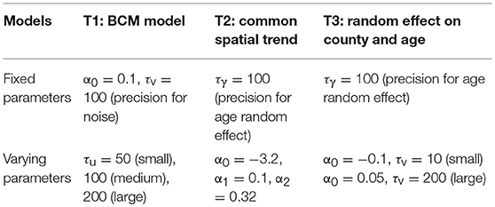
Table 1. Simulation scenarios and parameters.
The first 100 of the 1,000 simulated datasets are used to evaluate the performance of the four methods. The evaluation criteria include: (1) mean length of 95% interval estimate (CI); (2) coverage probability, measured by the proportion of overlap between 95% intervals from the simulated datasets and the model fitted 95% intervals; and (3) measure of variability, which is the standard deviation of CI length. Only the first 100 simulated datasets are used due to the lengthy computation time in BCM model. It took 4 weeks to run BCM using the 100 datasets for each of the six simulation scenarios and common (Count = 13,000) or rare (Count = 3,000) diseases.
The results of the simulation study are presented in Table 2 (Count = 13,000) and 3 (Count = 3,000). The four methods are compared based on the length of the interval estimates, the coverage probability, and the standard deviation of the intervals. A narrower interval indicates more liberal estimation. Coverage probability is supposed to be close to 95%. Standard deviation of the intervals indicates variation of the interval estimates. Since the data are simulated according to the Kentucky population, the 120 counties in Kentucky are categorized according to the size of the county population. The 40 large counties have an average population of 191 k, the 40 medium counties have an average population of 48 k, and the 40 small counties have an average population of 24 k. Within each simulation scenario, large counties tend to have more liberal interval estimates, with coverage probability closer to 95%, and variation of interval length tend to be small. There is an obvious improvement in the interval estimates from the Direct method to the Overlap method to the Spatial method, especially when the precision of spatial random effect is large compared to medium or small values. Compared to other methods, BCM model has the largest average CI length and variability of the CI length across all simulation scenarios (Tables 2, 3). When the data were simulated under the spatial convolution model with a very precise correlated spatial effect (i.e., large tau), the BCM approach yields the largest coverage probability among all methods. For all simulation scenarios, the length of CI decreases as population size increases. The performance of each method becomes worse as the precision of the parameters decreases.
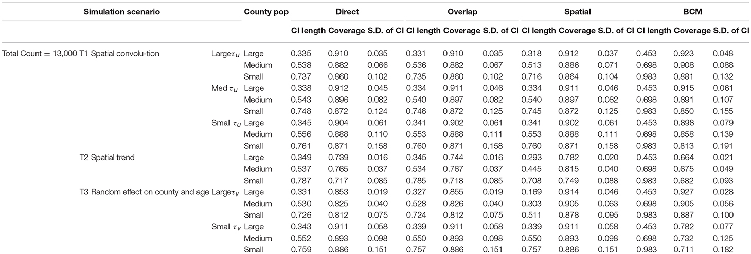
Table 2. Comparison of four methods under 6 data simulation scenarios for total count at 13,000.
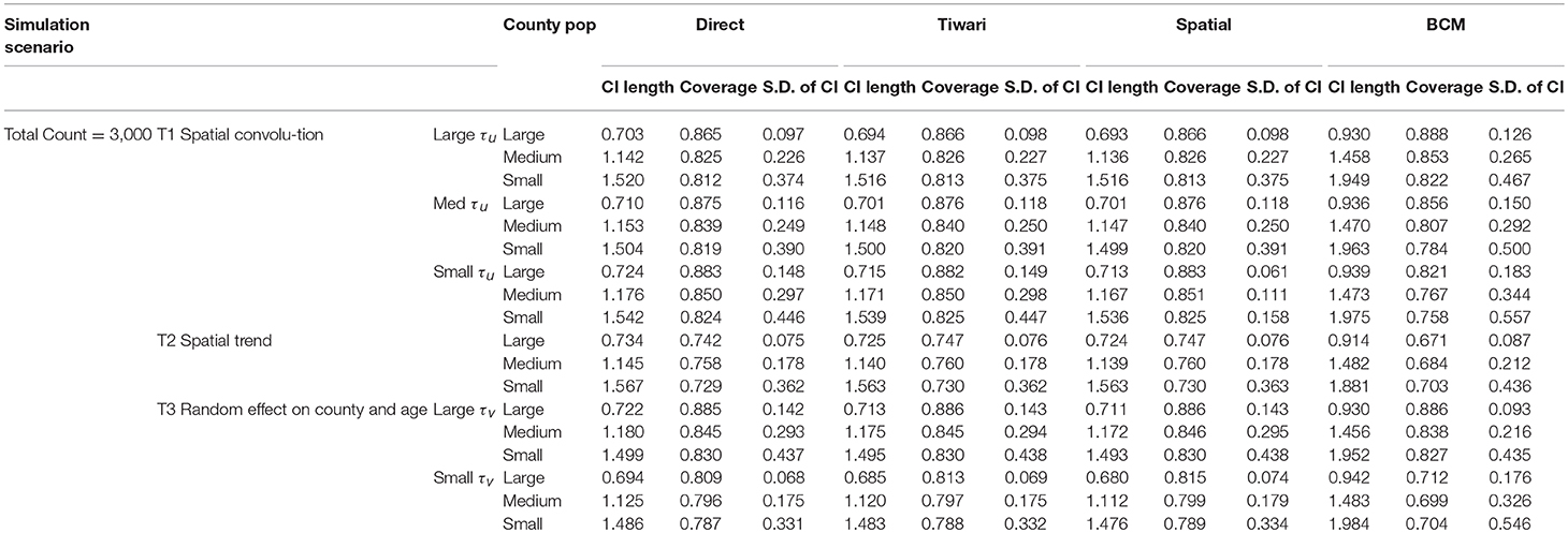
Table 3. Comparison of four methods under 6 data simulation scenarios for total count at 3,000.
Application Examples
Comparison of the four methods was made using cancer incidence data from the National Cancer Institute's Surveillance, Epidemiology and End Results (SEER) Program. SEER collects data on cancer cases from various locations and sources throughout the United States. This program currently collects and publishes cancer incidence and survival data from state and metropolitan level population-based cancer registries covering ~30% of the US population. The data is released through statistical software SEER*Stat (15) for the analysis of SEER and other cancer-related databases, such as mortality and county attributes. SEER*Stat calculates the non-adjusted and age-adjusted rates (AARs) of cancer incidence or mortality, as well as the rate ratio and the 95% CIs of the RR between selected geographic areas using the Direct method.
Using dataset released in the SEER*Stat software (16), we analyze the Kentucky male lung cancer and oral cancer (both genders) incidence data (Data has been provided in the Supplementary Material section) to obtain model-based age adjusted rate and county-to-state RR with associated credible intervals. The state of Kentucky has the highest cancer rates for both incidence and mortality. Cigarette smoking and tobacco chewing prevalence are high, especially in the southeast area of the state which is part of the Central Appalachia region (17). Tobacco use causes many types of cancer, including cancer of lung, mouth, esophagus, throat, bladder, and pancreas (18). We calculate the age-adjusted incidence rates of lung cancer (male only) and oral cancer (both genders) for the 5-year period between 2006 and 2010. These two cancer sites are selected to represent a more common and a rare cancer, respectively. The lung cancer state rate is 126.94 per 100,000 and the rates vary considerably among the 120 counties, from 57.01 to 207.21 (Figure 1, Direct), resulting in the county-to-state RR between 0.45 and 1.63 (Figure 2, Direct). There is also a spatial pattern, with higher rates in the southeast mountain area, and lower rates in the north and central areas. The oral cancer state rate is 13.12 and the county rates vary between 3.96 and 30.80 (Figure 3, Direct). The county to state RR range between 0.30 and 2.35 (Figure 4, Direct).
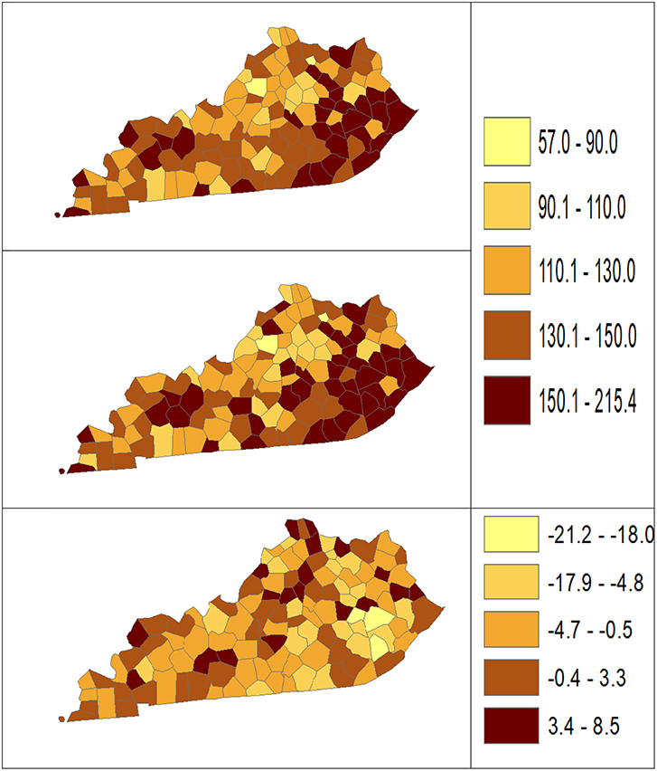
Figure 1. Age-adjusted rate estimated from statistical methods (Direct top vs. BCM middle) and their difference (bottom) using 2006–2010 lung cancer incidence data in Kentucky counties.
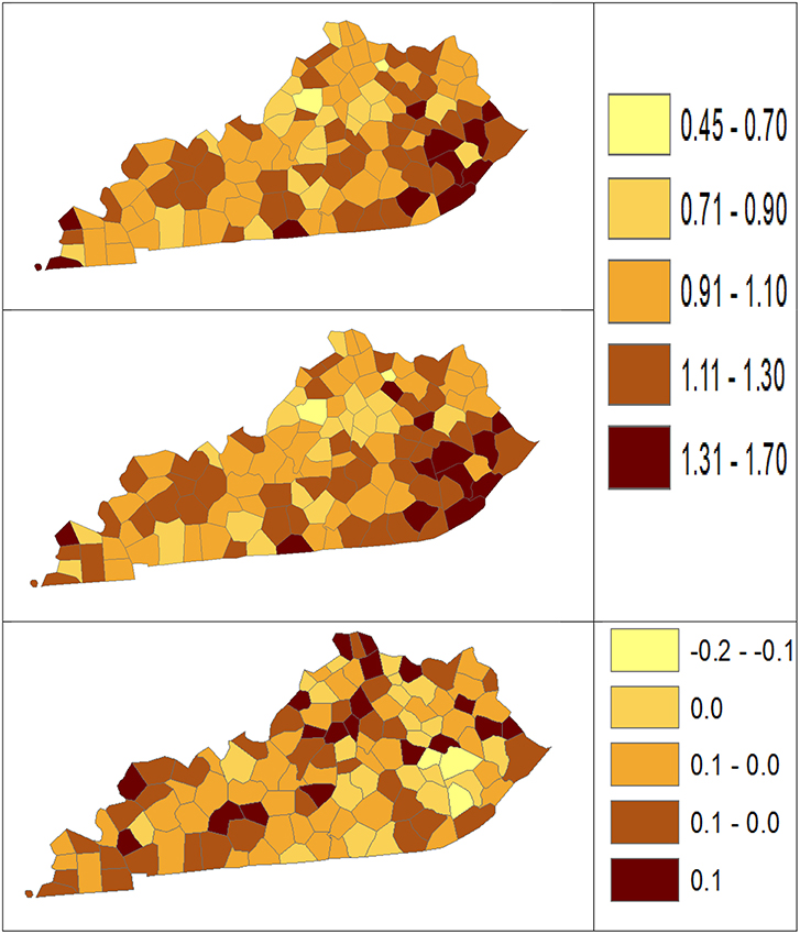
Figure 2. Rate ratio estimated from statistical methods (Direct top vs. BCM middle) and their difference (bottom) using 2006–2010 lung cancer incidence dataset.
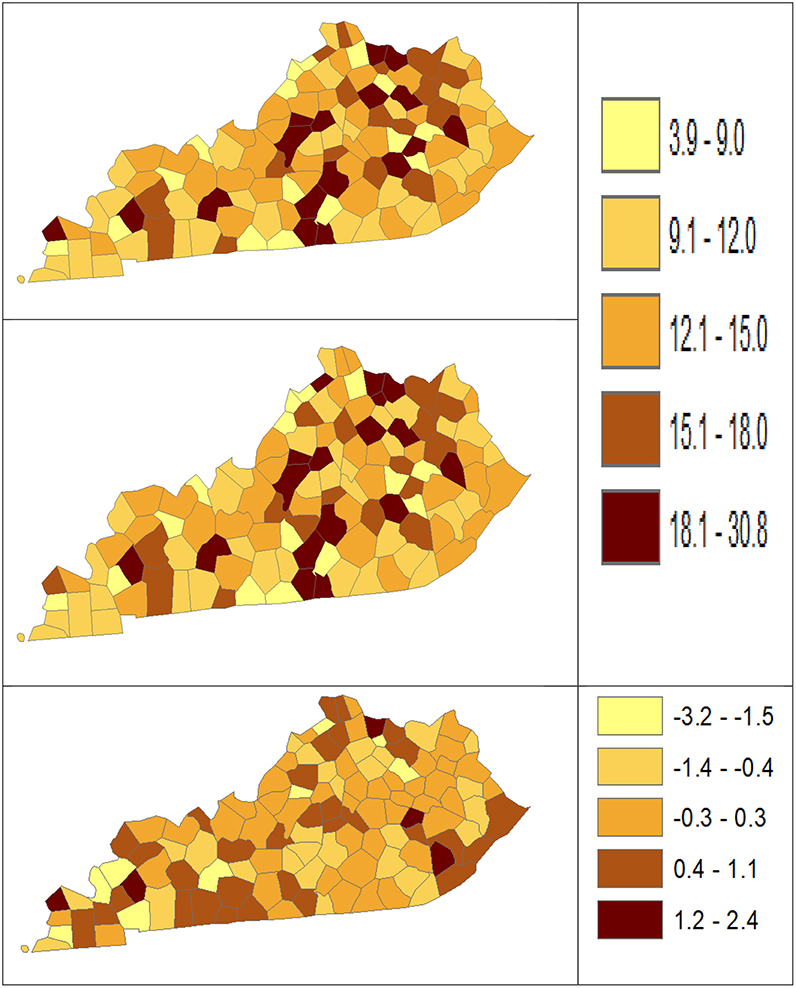
Figure 3. Age-Adjusted Rate estimated from statistical methods (Direct top vs. BCM middle) and their difference (bottom) using 2006–2010 oral cancer incidence dataset.
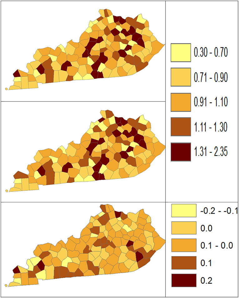
Figure 4. Rate Ratio estimated from statistical methods (Direct top vs. BCM middle) and their difference (bottom) using 2006–2010 oral cancer incidence dataset.
The population nij and number of cases Dij in each region and age strata are read in the matrix of I (region) rows and J columns for each age specific count, with each region associated with a unique index (FIPS code). For each region and age stratum, the expected number of cases eij is computed using reference rates for the disease incidence: . To fit the joint model to obtain posterior mean and distribution of the relative risk λij, observed count and expected count with adjacency matrix are entered into the MCMC algorithm. The adjacencies for the CAR prior distribution are computed from the county or state maps using R functions in library maps, maptools, and library spdep. The program used for conditional autoregression model analysis is self-written MCMC algorithm function based on BCM using the R language (19).
Results
Table 4 shows the point and interval estimates of AARs and RR using all four methods, for the top, middle, and lowest 5 RR of lung cancer incidence data in Kentucky counties. The interval estimates showed shrinkage from the Direct to the Overlap and to the Spatial method. By contrast, the BCM method yields different point estimates but a wider interval length as BCM incorporates the uncertainty from spatial random effect, so the interval estimate for BCM is wider. Overall, BCM provides a smoothing effect by considering the neighborhood information for the point estimates of relative risk estimates, especially for the regions with small counts. The point estimates of the AAR from BCM model algorithm are close to those from the Direct estimate (Table 4): the difference in overall rate is 0.02 and mean difference in the AAR of all regions is 1.21. The mean rate ratio difference between two methods is also minimal (0.01). However, the interval length of BCM algorithm is greater than that is calculated from the “Direct” method, for both rate and RR.
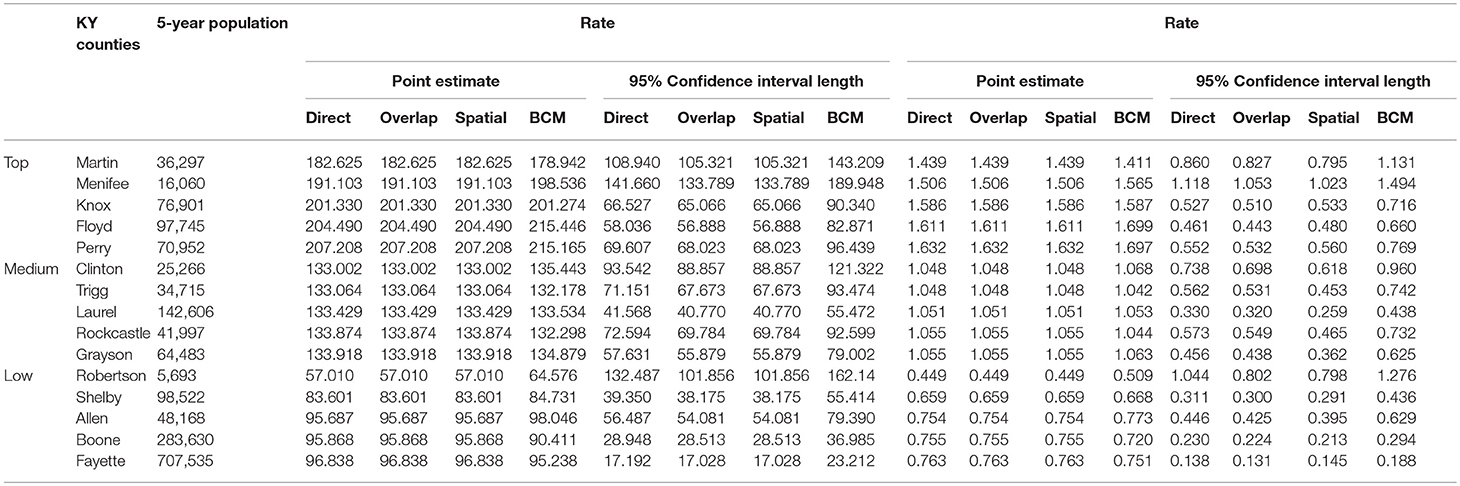
Table 4. Age-adjusted rate and rate ratio in top, middle, and bottom five counties based on 2006–2010 lung cancer incidence rate in Kentucky.
The Bayesian disease-mapping analyses for lung cancer data are presented in Figures 1, 2, which displayed the point estimate of the age-adjusted mortality rate, the rate ratio, and the difference between the direct and BCM methods (BCM minus direct) for each area based on 2006–2010 lung cancer incidence dataset. BCM provides a “smoothing” effect for the point estimates. Specifically, in eastern Kentucky, estimated region-specific AARs are higher (shaded in a darker color) based on both the direct and BCM methods. In the difference maps, the eastern Kentucky is shown in a lighter shade, meaning BCM produces lower estimates toward an overall smoothing average. By contrast, there are more areas with lower rate estimates (shaded in lighter color) in the western regions after controlling for spatial correlations. However, overall, BCM maintains “appearance” of the direct estimation while producing “smoothing” effect for the regions with extreme (high or low) rates by considering the neighborhood information.
Table 5 shows the point and interval estimates of AARs and RR using all four methods, for the top, middle, and lowest 5 RR of oral cancer incidence data in Kentucky counties. Similar to the lung cancer example, the oral cancer overall rate and region-specific AAR (and the rate ratios) yielded from BCM model are similar to the direct estimates. Fewer extreme rates are shown in the map (Figures 3, 4) produced from BCM model as compared to the map from direct estimates. The difference between the BCM and the direct estimates (bottom maps in both Figures 3, 4) shows an opposite distribution pattern, indicating the smoothing effect of the BCM method. In terms of variation, BCM method provides a wider interval than the Direct estimates for both rate and rate ratio estimates (Table 5).
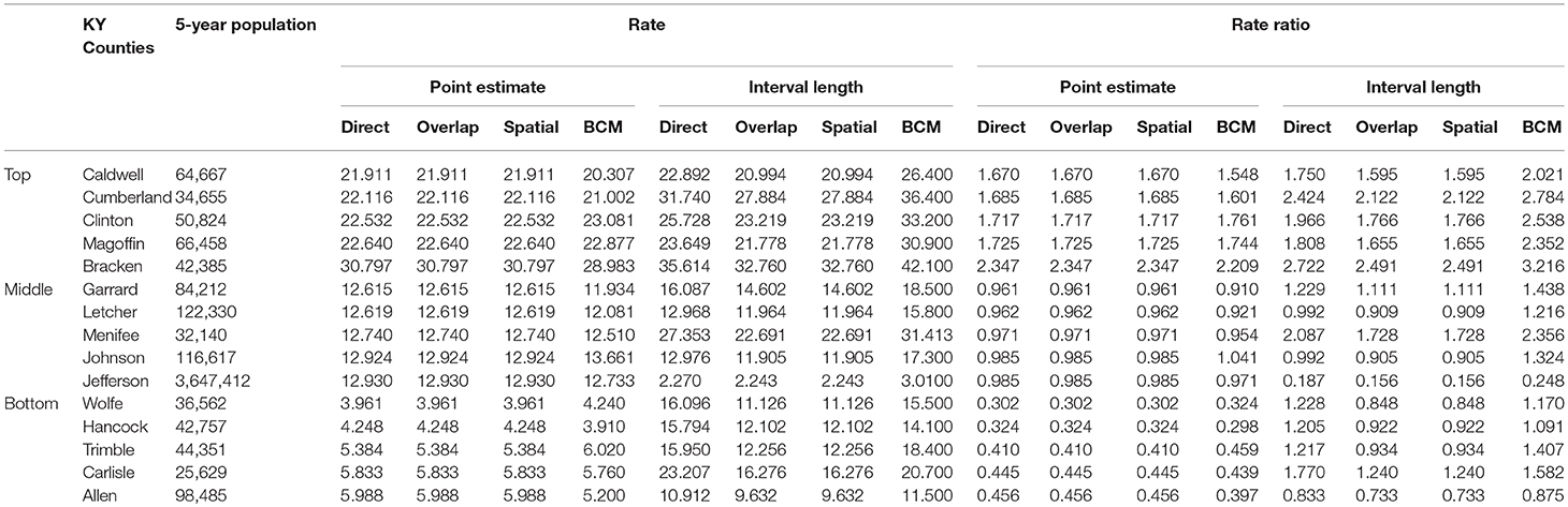
Table 5. Age-adjusted rate and rate ratio in top, middle, and bottom five counties based on 2006–2010 oral cancer incidence rate in Kentucky.
To further compare the direct method and BCM model, we plot the interval length of RR between direct method and BCM model for both lung and oral cancer datasets (Figure 5). In both datasets, there is a remarkably high correlation between direct and BCM estimation. For lung cancer dataset with larger number of events, there is 30% difference in the length of RR intervals between Direct and BCM model, and on average BCM yields wider intervals as compared to the direct estimation. For oral cancer dataset, the difference in length of RR interval is < 10% between direct and BCM estimation. To make a valid comparison between the Direct and the BCM estimates on the common scale, we first standardized the interval length for RR from each method into z-scores by subtracting the mean and dividing by the standard deviation. Secondly, we applied the regression technique based on iterated re-weighted least squares (IRLS) with reweighted observations according to their absolute residuals. After standardization, there is almost a perfect correlation (99%) between two methods, the distributions of the interval length of the rate ratio are very close for both datasets (Figure 6). In other words, the county with the widest CI from the Direct method also has the widest CI from BCM estimation.
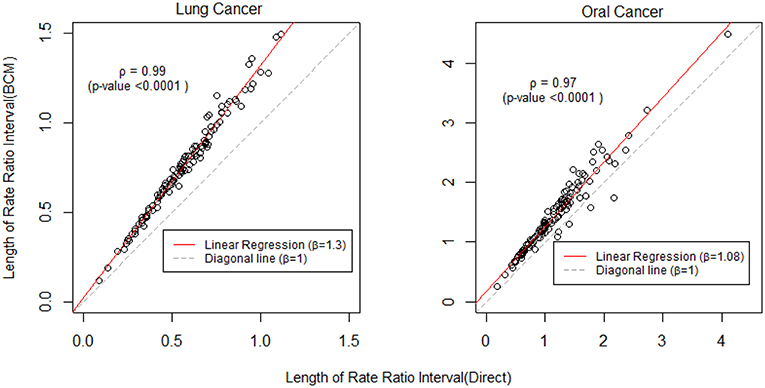
Figure 5. The comparison of rate ratio interval length between Direct method and BCM model (Before standardization). β is the slope for regression and ρ is the bivariate correlation.
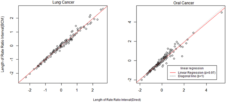
Figure 6. The comparison of rate ratio interval length between Direct method and BCM model (After standardization). β is the slope for regression.
We compare the interval length estimates across four different methods (Figure 7). The interval length for the rate ratio shrinks from the Direct method, to the Overlap method and to Spatial method in both oral and lung cancer analyses. BCM method produces the widest CI for rate ratio in both oral and lung cancer datasets. The median rate ratio tends to be greater with BCM model as compared to the other methods.
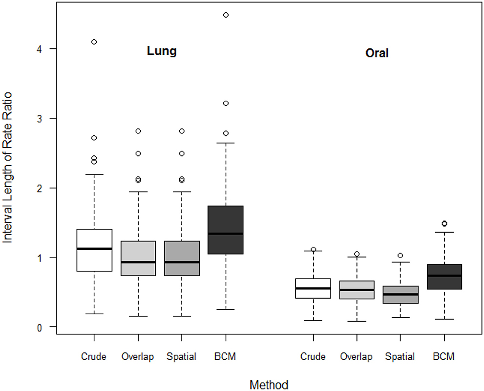
Figure 7. Boxplot of lengths of 95% CI for Rate Ratio by cancer site (oral or lung cancer) and method.
Discussion
In this study, the BCM method is implemented to analyze the Kentucky male lung cancer and oral cancer (both genders) incidence data acquired from the NCI SEER program, with the goal of obtaining the model-based age adjusted rate and county-to-state RR with associated credible intervals by properly taking into consideration the spatial correlation patterns. BCM allows for incorporating both uncorrelated and correlated spatial heterogeneity according to an existing neighborhood structure. Among the different methods, the Overlap and Spatial methods yield the same point estimates of rate or RR, only the interval estimates show shrinkage from the Direct method, to the Overlap and the to the Spatial method. By comparison, the proposed BCM method produces the similar point estimates for rate and RR, but since this method incorporates the uncertainty from the spatial random effect, this leads to a much wider 95% CI for the RR.
Both the Spatial method and BCM consider the spatial correlation for estimating a CI for RR. For both datasets, BCM produces a much wider 95% CI for the RR, which is predominantly larger for lung cancer (higher count of events) as compared to oral cancer (small count of events) data, while the Spatial method has a shrinkage effect for the interval estimates in lung cancer data but not for oral cancer data. Unfortunately, there is little literature on the difference in interval width for comparing BCM methods to non-spatial methods. The exception is Best et al. (20) where they cite CV (coefficient of variation) for different methods but do not assess the addition of a spatial effect. One obvious reason is that two approaches have different assumptions about the form of spatial structures—the spatial method hypothesizes a parametric exponential distribution for spatial correlation structure, and the convolution model estimates spatial correlation by assuming a conditional autoregressive (CAR) prior distribution. In addition, the 95% credible interval estimated from BCM is formed by Monte Carlo draws from the posterior distribution, which tends to include a random noise component in the interval estimation, and could potentially lead to a greater CI as compared to the numerical approximation as is defined in the spatial methods. As a side interest, we also compared the length of 95% CI in RR produced from UH model and BCM model. The boxplot (Figure A1) shows the UH and BCM model widths of 95% CIs for the relative risk for Kentucky counties: the overall width is greater for BCM model.
The main advantage of using BCM is to allow flexible modeling of spatial correlation in a natural way by including uncorrelated (UH) and correlated (CH) spatial heterogeneity. Secondly, the posterior sampling based on Monte Carlo simulation tends to be more accurate than the numerical approximation, and the distributions of all the parameter estimates and model information can be obtained. Further, simulation studies have shown that BCM outperforms other methods (non-parametric smoothing methods, marginal mixture models, and full Bayes models etc.) in the analysis of small area disease incidence data with respect to overall recovery of true risk (6).
As a limitation, the data example used in this study is specifically on cancer surveillance. A larger sample could be used to illustrate the application of the methodology in a broader area in public health. More practical applications will be needed to further evaluate the performance of Bayesian convolution model and demonstrate its effectiveness. Alternatively, approximate Bayesian Inference for Latent Gaussian Models can be also obtained using Integrated Nested Laplace Approximations (INLA) (6) which can yield improved computational efficiency.
Bayesian approaches to statistical problems have gained popularity in various fields, such as epidemiology, medical and public health. Most government sources hold publicly accessible aggregated health data due to confidentiality requirements. The resulting count data, usually available at county or postal/census region level, can yield important insights into the general spatial variation of disease in terms of incidence or prevalence. However, the novel application of spatial methodology is less well-recognized in this area and it is expected to improve the efficiency of analysis of clustering effect. Bayesian convolution model (BCM) is the fundamental strategy that can incorporate the uncorrelated and correlated spatial heterogeneity effect, the extension of this model can further take into account the unobserved confounding variables that have a spatial expression over the course of the study or conduct the longitudinal type analysis. A potential future direction in this research is to check the predictive validity through simulation study or bootstrap cross-validation, so that the method can be promoted for broader planning applications. Another future research focus of this work include the inclusion of clinical and registry-level analysis, as well as population level analyses resulting from cancer registry data, the data on health service utilization, and clinical trials.
Author Contributions
YJ developed the R program, provided analysis on the data example and results, and drafted the manuscript. AL advised the design and development of the method. LZ and EF provided guidance in developing the new method and summarized the existing methods. LZ also developed the simulation study. All authors reviewed and revised the manuscript and approved the final version.
Funding
This work was partly supported by the National Institutes of Health contract HHSN261201500388P.
Conflict of Interest Statement
The authors declare that the research was conducted in the absence of any commercial or financial relationships that could be construed as a potential conflict of interest.
Acknowledgments
This work was partly supported by the Statistical Methodology and Applications Branch of the National Cancer Institute through a contract HHSN261201500388P (contract number).
Supplementary Material
The Supplementary Material for this article can be found online at: https://www.frontiersin.org/articles/10.3389/fpubh.2019.00144/full#supplementary-material
References
1. Tiwari RC, Clegg LX, Zou Z. Efficient interval estimation for age-adjusted cancer rates. Stat Methods Med Res. (2006) 15:547–69. doi: 10.1177/0962280206070621
2. Tiwari RC, Li Y, Zou Z. Interval estimation for ratios of correlated age-adjusted rates. J Data Sci. (2010) 8:471–82. doi: 10.6339/JDS.2010.08(3).610
3. Zhu L, Pickle LW, Pearson JB. Confidence intervals for rate ratios between geographic units. Int J Health Geograph. (2016) 15:1–13. doi: 10.1186/s12942-016-0073-5
4. Besag J, York J, Mollie A. Bayesian image restoration, with two applications in spatial statistics. Ann Inst Stat Math. (1991) 43:1–20. doi: 10.1007/BF00116466
5. Earnest A, Morgan G, Mengersen K, Ryan L, Summerhayes R, Beard J. Evaluating the effect of neighbourhood weight matrices on smoothing properties of Conditional Autoregressive (CAR) models. Int J Health Geogr. (2007) 6:54. doi: 10.1186/1476-072X-6-54
6. Lawson AB, Biggeri AB, Boehning D, Lesaffre E, Viel JF, Clark A, et al. Disease mapping models: an empirical evaluation. disease mapping collaborative group. Stat Med. (2000) 19:2217–41. doi: 10.1002/1097-0258(20000915/30)19:17/18<2217::AID-SIM565>3.0.CO;2-E
7. Fay MP. Approximate confidence intervals for rate ratios from directly standardized rates with sparse data. Comm Stat Theory Methods. (1999) 29:2141–60. doi: 10.1080/03610929908832411
8. Fay MP, Feuer EJ. Confidence intervals for directly standardized rates: a method based on the gamma distribution. Stat Med. (1997) 16:791–801. doi: 10.1002/(SICI)1097-0258(19970415)16:7<791::AID-SIM500>3.3.CO;2-R
9. Tobler W. A computer movie simulating urban growth in the Detroit region. Economic Geography. (1970) 46:234–40. doi: 10.2307/143141
10. Matheron G Principles of geostatistics. Economic Geol. (1963) 58:1246–66. doi: 10.2113/gsecongeo.58.8.1246
12. Gotway CA, Stroup WW. A generalized linear model approach to spatial data analysis and prediction. J Agric Biol Environ Stat. (1997) 2:157–78. doi: 10.2307/1400401
13. Rotejanaprasert C, Lawson AB. A bayesian quantile modeling for spatiotemporal relative risk: an application to adverse risk detection of respiratory diseases in South Carolina, USA. Int J Environ Res Public Health. (2018) 15:E2042. doi: 10.3390/ijerph15092042
14. Lawson A, Banerjee S, Haining RP. Handbook of Spatial Epidemiology. Boca Raton, FL: Chapman and Hall/CRC (2016).
15. National Cancer Institute. SEER*Stat Software. (2018). Available online at: http://seer.cancer.gov/seerstat/
16. Surveillance Epidemiolgy and End Results (SEER) Program NCI SEER*Stat Database: Incidence–SEER 18 Regs Research Data + Hurricane Katrina Impacted Louisiana Cases, Nov 2013 Sub (2000–2011)<Katrina/Rita Population Adjustment>-Linked To County Attributes–Total U.S., 1969–2012 Counties. S.R.P. National Cancer Institute, Surveillance Systems Branch (2014).
17. Christian WJ, Huang B, Rinehart J, Hopenhayn C. Exploring geographic variation in lung cancer incidence in Kentucky using a spatial scan statistic: elevated risk in the appalachian coal-mining region. Public Health Rep. (2011) 126:789–96. doi: 10.1177/003335491112600604
18. International Agency for Research on Cancer. Smokeless Tobacco and Some Tobacco-Specific N-Nitrosamines, in IARC Monographs on the Evaluation of Carcinogenic Risks to Humans. Loyn: International Agency for Research on Cancer. (2007).
19. R Development Core Team. The R Project for Statistical Computing. (2016). Available online at: https://www.r-project.org/ (cited August 29, 2016)
20. Best N, Richardson S, Thomson A. A comparison of bayesian spatial models for disease mapping. Stat Methods Med Res. (2005) 14:35–59. doi: 10.1191/0962280205sm388oa
Appendix
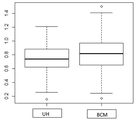
Figure A1. Boxplot of rate ratio CI width for comparing UH and BCM model using oral cancer incidence dataset.
Keywords: spatial correlation, rate ratio, Bayesian statistics, BCM model, CAR prior
Citation: Jiang Y, Lawson AB, Zhu L and Feuer EJ (2019) Interval Estimation for Age-Adjusted Rate Ratios Using Bayesian Convolution Model. Front. Public Health 7:144. doi: 10.3389/fpubh.2019.00144
Received: 16 November 2018; Accepted: 20 May 2019;
Published: 05 June 2019.
Edited by:
Jimmy Thomas Efird, University of Newcastle, AustraliaReviewed by:
Serdar Dindar, University of Birmingham, United KingdomJuan Pablo Carbajal, Swiss Federal Institute of Aquatic Science and Technology, Switzerland
Copyright © 2019 Jiang, Lawson, Zhu and Feuer. This is an open-access article distributed under the terms of the Creative Commons Attribution License (CC BY). The use, distribution or reproduction in other forums is permitted, provided the original author(s) and the copyright owner(s) are credited and that the original publication in this journal is cited, in accordance with accepted academic practice. No use, distribution or reproduction is permitted which does not comply with these terms.
*Correspondence: Li Zhu, li.zhu@nih.gov