Effective precursors for self-organization of complex systems into a critical state based on dynamic series data

1 Introduction

It was established more than 35 years ago that self-organization leads not only to the emergence of order in a nonlinear complex system and the separation of order parameters from the set of degrees of freedom, but also brings the system to a critical state (e.g., see the paper [1]). In such a state, catastrophic avalanches of any scale are possible, limited only by the size of the system. What is fundamentally important in such a phenomenon is that there is no need to tune the control parameter to a critical value, which is necessary for phase transitions. For example, the well-known paramagnetic-ferromagnetic phase transition of the second kind requires fine-tuning of temperature as a control parameter to a critical value. On the contrary, self-organized criticality (SOC) spontaneously arises as a result of many local interactions between the elements of the system. In the context of statistical physics of phase transitions, a system located in a small neighborhood of a critical point is unstable with respect to small perturbations capable of causing avalanches of any size in the system. Such a point separates disordered (the phase with a zero order parameter) and ordered (the phase with a non-zero order parameter) phases (see Figure 1C). It has been relatively recently established (e.g., see papers [2, 3]) that complex systems are not only capable of self-organization at a critical point, but also capable of self-organization into a state characterized by two stable configurations. Self-organized bistability (SOB) demonstrates the coexistence of two stable configurations in the hysteresis loop ($L_1{L}_2{L}_3{L}_4$) corresponding to zero order parameter and non-zero order parameter (see Figure 1A). Let us consider the transitions between the ordered and disordered phases occurring in the loop $L_1{L}_2{L}_3{L}_4$. If the system is in the state $L_1$, If the system is in the state $L_1$, the system remains in the unordered phase until the point $L_2$ when the control parameter is increased. Then the system jumps to the $L_3$ point. Such a transition corresponds to a sharp increase in the ordering of the system. When control parameter decreases, the system moves to point $L_4$ with decreasing orderliness of the system. Further decrease of the control parameter sharply moves the system to point $L_1$, corresponding to the unordered state of the system. The SOB is associated with a phase transition of the first kind, such as the liquid-vapor transition at a jump-like change of the order parameter (see the paper [2]). Recently, numerous evidence of self-organization of real-world systems of various origins into a critical state have been obtained. SOC is characteristic of financial markets (e.g., see papers [4–6]), social interaction networks (e.g., see papers [7–9]), epidemiological complex networks (e.g., see papers [8, 10]) and many other systems of very different origin (e.g., see papers [8, 11]). SOB is characteristic of the brain (e.g., see the paper [12]). In the following, the SOC state will be understood as the state of the system staying in the critical point; the SOB state will be understood as the state of the system staying in the region of the hysteresis loop.

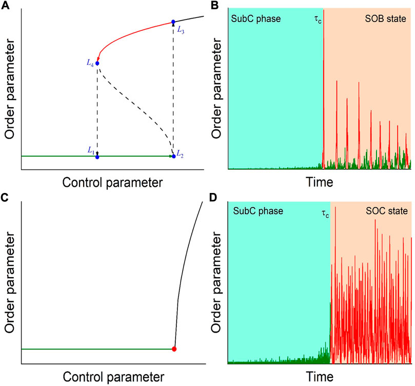
FIGURE 1. Mean-field phase diagrams showing self-organization into bistable (A) and critical (C) states, and time series for the order parameter corresponding to self-organization into bistable (B) and critical (D) states. The hysteresis loop is shown by arrows. The symbol ${\mathrm{\tau }}_{\mathrm{c}}$ indicates the critical time that separates the subcritical phase and the critical state.

The basic model of self-organization of systems into a critical state is the sand pile model (e.g., see the paper [13]), which is formulated as a two-dimensional cellular automaton. Such a model describes a variety of processes in complex systems that self-organize into a critical state and reflects typical properties and features of real-world systems of various origins, such as stock exchanges and online social networks (see section “Conclusion”). The simplest sand automaton is a square grid whose nodes contain an integer number of grains of sand. New grains of sand fall on randomly selected nodes. If the number of grains of sand in each node is at most three, the automaton is in a stable state. As soon as a fourth grain of sand falls into one of the nodes, a collapse occurs. The grains of sand from this node are redistributed to neighboring nodes, which can cause collapses in them. Collapses will avalanche until the automaton returns to a steady state again (see Figures 1B, D). Despite the fact that such an automaton is a model system with local rules, i.e., the nodes of the automaton are only capable of interacting with their nearest neighbor nodes, it exhibits complex behavior. In other words, complexity is born from simple elements as a result of self-organization. It is in this context that we consider sand cellular automata as complex model systems. This is the classical model of self-organized criticality proposed by P. Buck, C. Tang, and C. Wiesenfeld in 1987 (see the paper [1]), which demonstrates the transition of an automaton from a subcritical (disordered) phase to a critical state.

One of the problems in the development of early warning systems, which has not been finally solved, is finding effective precursors of the system transition to a critical state, known as the early warning signals (e.g., see papers [14–20]). First of all, it is the search for precursors based on the analysis of the observed sequence of values of a macroscopic variable, usually an order parameter, generated by the system in real time. One of the results of research directly or indirectly related to the analysis of real-time dynamical series is the measures, by the characteristic change of which one can judge about the approach of the system to the critical transition point. Further in this paper we will call such measures the early warning measures (EWM). First of all, these are the EWMs, the change of which is explained by the increase of the relaxation time of the system near the critical point. This is known as the phenomena of critical slowing down (e.g., see the paper [21]). EWMs have also been proposed that are not directly related to this phenomenon, but their characteristic change near the critical point can be considered as the early warning signals for the critical transition (e.g., see the paper [15]). The number of EWMs and systems for which EWMs give good results in predicting critical points is regularly growing.

Despite the available variety of precursors of self-organized critical transitions based on EWMs, not all precursors can be considered as effective. Even the best-studied precursors based on variance and autocorrelation at lag-1 are not effective for all systems. Moreover, the effectiveness of the precursor depends on the origin of the real-world system and/or on local and global features of the observed sequence of values of the macroscopic variable. In the context of early warning systems, we relate the effectiveness of the precursor to the sufficiency of time from the moment of its occurrence to the transition of the system to a critical state for decision making, as well as to the absence of false positive and/or false negative results of early detection.

To date, we are not aware of any work that presents a study of the above-defined efficiency of precursors of self-organized critical transitions. To close this gap, we have investigated the efficiency of various EWMs of dynamical series of the number of unstable nodes of sand cellular automata. To ensure the representativeness of the results obtained, we investigated the effectiveness of not only the most studied EWMs, such as some sample moments, autocorrelation, and the power-law exponent of the spectral density, but also little or no studied EWMs, such as measures related to wavelet transform, and phase space reconstruction from the time series data. In addition, representativeness was ensured by the diversity of topological structure of graphs, local rules, and types of pumping of cellular automata. The choice of sand cellular automata from the existing model systems with SOC and SOB is due to the fact that for them the iteration corresponding to the output of the automaton to the critical state is precisely known, so it is possible to precisely determine the prediction time as one of the criteria for the effectiveness of the measure. Finally, in the context of systems theory, such automata are isomorphic to real-world systems, for which there is a need to perform a real-time study of the critical state exit from the moment they start pumping.

The paper is structured as follows: first, a short introduction to the sandpile cellular automata, including the local rules, graph topologies and external pumping used in this study, and the rationale for choosing such automata as test models to study precursors in real systems are described. Next, a formal definition of an effective precursor to an effective EWM in the context of early warning systems is presented. Also the investigated EWMs and methods of their computation are described. All this is presented in section “Data set and methods”. Finally, the results of computing EWMs depending on the rules, topology and pumping of automata are presented and discussed, as well as the possibilities and limitations of using such measures to detect effective precursors of critical transitions (see section “Results and discussion”). In addition, the possibilities and limitations of using effective precursors for early detection of critical transitions in complex systems are described, as well as possible practical applications of the results obtained (see section “Conclusion”).

2 Methods

As mentioned in section “Introduction”, we investigate the effectiveness of EWMs to self-organize sand cellular automata into a critical state based on the behavior of discrete dynamical series for unstable automata nodes. These are the dynamical series $\left\{{\xi }_t|t\in \left[0,n\right],n\in \mathbb{N}\right\}$, where ${\xi }_t$ is the number of unstable nodes of the automaton in t-th iteration. In the presented study, we use the most common window measure m, which is computed in a window of fixed width $w_0\in N$. By sliding such a window along a series ${\xi }_t$ with the computation of m for each window shifted by one iteration step, starting from window $\left[{\xi }_0,{\xi }_{w_0}\right]$, we obtain a dynamic series of measures $\left\{{\mathcal{m}}_t|t\in \left[0,n-{\mathcal{w}}_0\right]\right\}$. The characteristic behavior of the series $m_t$, or zero-mean dynamic series of increments $\left\{∆{\mathcal{m}}_t=\left({\mathcal{m}}_{t+1}-{\mathcal{m}}_t\right)/{\mu }_t|t\in \left[0,n-{\mathcal{w}}_0\right]\right\}$, as $t$ approaches the moment of the critical transition ${\tau }_c$ is a harbinger of the self-organization of the automaton into the critical state. The mean ${\mu }_t$ is calculated for the values of the series ${\xi }_t$ in each window.

2.1 Sandpile cellular automaton as a generator of dynamic series data

Consider a sand cellular automaton on a planar graph $\mathrm{\Gamma }$ with nodes $\left(i,j\right)$ in the plane for which $i,j\in Z$. The most studied automata on square grid graphs (SGG) are of little use as models of real world systems. This is primarily due to the fact that the propagation of sand grains from an unstable node $\left(i_u,j_u\right)$ as a result of its collapse is only possible to its four nearest neighbor nodes $\left(i_u\pm 1,j_u\pm 1\right)$. For this reason, we also investigated the critical behavior of automata on the Erdos-Renyi graph (ERG) and the Chung-Lu graph (CLG). Thus, ERG has been successfully applied in modeling the dynamics of opinions in financial markets (e.g., see the paper [6]), CLG in modeling information dissemination in online social networks (e.g., see the paper [22]). An ERG is a random graph on $n$ nodes $\left(i,j\right)\in Z$, in which an edge $\left(k,m\right)$ between two nodes $\left(i_k,j_k\right)$ and $\left(i_m,j_m\right)$ appears independently of all other pairs of nodes with equal probability $p$. The degree distribution of the nodes of the graph is binomial with parameters $n-1$ and $p$. In CLG, each vertex is assigned a weight, and each pair of nodes is associated with a probability proportional to the product of their weights. In the resulting graph, each vertex has an expected degree equal to its weight. Growing a CLG consists of several steps. Let $V=\left\{v_k=\left(i_k,j_k\right)|k\in \left[1,n\right],n\in \mathbb{N}\right\}$ and the degree of each node $d_k,t\in \left[1,n\right]$. In the first step, we create a set $L$, consisting of $d_k$ copies of $v_k$ node for each $k=\overline{1,n}$. In the second step, we define random pairwise combinations on the set $L$. For nodes $v_i,v_j\in V$, the number of edges in CLG connecting them is equal to the number of vapor-combinations between their copies in $L$. The degree distribution of the nodes of the graph is a two-parameter degree distribution: $P\left\{\mathrm{deg}v=k\right\}=e^{\alpha }/k^{\beta }$, where $\alpha$ is the intercept for the power law distribution, $\beta >0$ is the slope for the power law distribution.

First, let us consider the processes occurring in the automaton on SGG, as well as its self-organization in the SOC state. Let initially nodes $\left(i,j\right)$ of the graph $\mathrm{\Gamma }$ are assigned numbers $z_{ij}\in Z^{+}\cup \left\{0\right\}$. In the context of sandpile cellular automata, number $z_{ij}$ corresponds to the number of sand grains in node $\left(i,j\right)$. An automaton is in a stable state if the inequality $z_{ij}<z_c$. Then, for automata on SGG we take the stability threshold $z_c=4$. The critical state of the automaton is reached as a result of an iterative sequence of disturbance and relaxation processes. The disturbance consists in that at the beginning of each new iteration the automaton is pumped up by assigning non-negative integers $z_{ij}$ to the nodes according to a certain pattern. The relaxation process starts, if for some node $\left(i_u,j_u\right)$ the inequality $z_{i_u{j}_u}\ge 4$ is fulfilled, then such a node transfers some number of grains of sand to neighboring nodes according to local rules of the model and the automaton passes to an unstable state. Such transfer of grains of sand can violate the stability of neighboring nodes, which can lead to an avalanche of node rollovers. The avalanche-like dynamics of the automaton continues until it returns to the stable state ($z_{ij}<4$ for all $\left(i,j\right)$). After that, the relaxation of the automaton is completed and a new pumping starts in the next iteration.

For all the automata studied, we used local rules of isotropic (non-directional) models. These are the Bak-Tang- Wiesenfeld (BTW) [1], Manna (MA) [23], and Feder-Feder (FF) [24] models. In the deterministic BTW and FF models, sand grains from unstable node $\left(i_u,j_u\right)$ are transferred to SGG equally to each of the four nearest four nodes of the square lattice, i.e., $z_{i_u\pm 1,j_u\pm 1}\to z_{i_u\pm 1,j_u\pm 1}+1$ (see Figures 2A, C). If we consider the collapses and redistribution of grains of sand presented in Figures 2A, C as processes occurring at some $k$-th iteration of the critical dynamics of the automaton, then such iteration can be considered as completed before complete relaxation. The number of unstable nodes of the automaton at the $k$-th iteration is ${\xi }_k=2$. In the stochastic MA model on SGG the nearest neighboring nodes with node $\left(i_u,j_u\right)$ get ${\delta }_k$ grains of sand, i.e., $z_{i_u\pm 1,j_u\pm 1}\to z_{i_u\pm 1,j_u\pm 1}+{\delta }_{i_u\pm 1,j_u\pm 1}$. Here ${\delta }_{i_u\pm 1,j_u\pm 1}\ge 0$ is a random number of grains of sand for which the equality ${\delta }_{i_u+1,j_u+1}+{\delta }_{i_u+1,j_u-1}+{\delta }_{i_u-1,j_u+1}+{\delta }_{i_u-1,j_u-1}=4$ (see Figure 2B). In the conservative BTW and MA models, when $\left(i_u,j_u\right)$ collapses, the number of grains of sand in it decreases by $z_c=4$, that is, $z_{i_u{j}_u}\to z_{i_u{j}_u}-4$ (see Figures 2A, C). For the dissipative FF model the number of grains of sand in $\left(i_u,j_u\right)$ goes to zero, i.e., $z_{i_u{j}_u}\to 0$ (see Figure 2C).

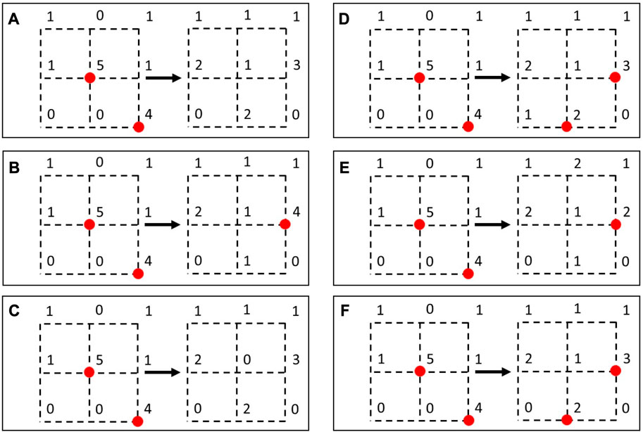
FIGURE 2. Collapse of the unstable vertice (shown in red) in the self-organized critical Bak-Tang-Wiesenfeld model (A), self-organized critical Manna model (B), self-organized critical Feder-Feder model (C), self-organized bistable Bak-Tang-Wiesenfeld model (D), self-organized bistable Manna model (E), and self-organized bistable Feder-Feder model (F).

The above described critical dynamics of the automaton on SGG corresponds to its exit to the SOC state. To exit the automaton to the SOB state, it is sufficient to set the stability threshold equal to $z_b$ ($z_b<4$) for nodes that received sand grains as a result of shattering of more than one neighboring node. We used $z_b=2$. In such an automaton, collapses of nodes $\left(i_u,j_u\right)$ occur when $z_{i_u{j}_u}\ge 4$, and when more than one sand grain from neighboring nodes is transferred to other nodes $\left(i,j\right)$. The collapses under the local rules of BTW, MA and FF models are shown in Figures 2D–F.

The difference between the local rules of automata on random graphs and the considered rules of automata on SGG is only in the choice of threshold values $z_c$. The value of $z_c$ is taken equal to the degree of node $\left(i_u,j_u\right)$. This is the value of a random variable from the binomial distribution of node degrees for the automaton on ERG, and the value of a random variable from the degree distribution of node degrees for the automaton on CLG.

In addition to the local rules of automata and graphs on which the collapse of unstable nodes and redistribution of sand grains between nodes occur, it is necessary to describe the rules of sand grains throwing in at each iteration, i.e., the pumping of the automaton. We performed automata pumping to its randomly selected nodes with the number of sand grains thrown in from discrete uniform distribution (DUD) with $a=0$ and $b=2$, exponential distribution (EXD) with $\lambda =1$, and Pareto distribution (PAD) with $\alpha =2$ and $x_m=0.475$.

2.2 Effectiveness of early warning measure

Let us introduce the notion of an effective EWM. Let, $\left\{∆{\mathcal{m}}_t|t\in \left[0,n-{\mathcal{w}}_0\right]\right\}$ be the zero-mean dynamic series of EWM increments for the dynamic series of the number of unstable nodes of the automaton $\left\{{\xi }_t|t\in \left[0,n\right]\right\}$, computed in a sliding window of width $w_0$; ${\tau }_c$ is the time when the system enters the critical state.

In addition, we introduce the following notations.

${\sigma }_0$ is the standard deviation of the series $∆m_t$ in the initial window $\left[{\xi }_0,{\xi }_{w_0}\right]$.

$-k_0{\sigma }_0$ and $k_0{\sigma }_0$ are the lower and upper control bounds for the series $∆m_t$. If the values of the series $∆m_t$ in the initial window have a normal distribution with zero mean, then $k_0=3$ (see $3\sigma$ rule). In the general case the distribution is not normal. Therefore, we chose for each measure such a value of $k_0\in R^{+}\cup \left\{0\right\}$, that would ensure that 99.9% of the values of the $∆m_t$ series in the initial window belong to the interval $\left(-k_0{\sigma }_0,k_0{\sigma }_0\right)$ (see Figure 3B).

$-2k_0{\sigma }_0$ and $2k_0{\sigma }_0$ are the lower and upper pre-warning bounds for the series $∆m_t$. The belonging of $∆m_t$ to the interval $\left(k_0{\sigma }_0,2k_0{\sigma }_0\right)$ and/or to the interval $\left(-2k_0{\sigma }_0,-k_0{\sigma }_0\right)$ is a pre-precursor of possible approach of the system to ${\tau }_c$. The precursor can be either false or true (see Figure 3B). False/true is determined by the further behavior of the $∆m_t$ series beyond the pre-warning boundaries.

$-3k_0{\sigma }_0$ and $3k_0{\sigma }_0$ are the lower and upper warning bounds for the series $∆m_t$, the introduction of which allows us to distinguish between false and true pre-warnings. If the sequence $\left\{∆m_k,∆m_{k+1},\dots ,∆m_{k+m}\right\}\in \left(0\right.,\left.k_0{\sigma }_0\right]\cup \left(k_0{\sigma }_0\right.,\left.2k_0{\sigma }_0\right]\cup \left(2k_0{\sigma }_0\right.,\left.3k_0{\sigma }_0\right]\cup \dots \cup \left(\left(n-1\right)k_0{\sigma }_0\right.,\left.n{k}_0{\sigma }_0\right]$, then the pre-precursor of the critical transition of the system is true. In such a case, $\left(k+m\right)$-th iteration corresponds to early warning time $\left({\tau }_{ew}\right)$ for the critical transition of the system at time ${\tau }_c$ (see Figures 3A, B). Otherwise, the pre-precursor is false. Figure 3B shows two false the pre-precursors from the interval $\left(k_0{\sigma }_0,2k_0{\sigma }_0\right)$ and one false the pre-precursor from the interval $\left(-2k_0{\sigma }_0,-k_0{\sigma }_0\right)$. The true warning discussed above corresponds to the increasing sequence $\left\{m_k,m_{k+1},\dots ,m_{k+m}\right\}$. By similar reasoning we can introduce the notion of a true warning for a decreasing sequence.

$\mathrm{{\rm M}}=\left\{{∆m}_t^{\left(1\right)},{∆m}_t^{\left(2\right)},\dots ,{∆m}_t^{\left(p\right)}\right\}$ is a set of series $∆m_t$. Each of such series demonstrates the behavior of some measure that characterizes a certain property of the series ${\xi }_t$ (see next Subsection).

$\mathrm{{\rm T}}=\left\{{\tau }_{ew}^{\left(1\right)},{\tau }_{ew}^{\left(2\right)},\dots ,{\tau }_{ew}^{\left(p\right)}\right\}$ there are multiple early warning times in the early warning measures of set $\mathrm{{\rm M}}$.

$\mathrm{{\rm N}}=\left\{{\nu }_f^{\left(1\right)},{\nu }_f^{\left(2\right)},\dots ,{\nu }_f^{\left(p\right)}\right\}$ there are multiple numbers of false pre-warnings in early warning measures from set $\mathrm{{\rm M}}$.

FIGURE 3. Early warning measure time series (A) and corresponding zero-mean time series (B). The symbols ${\mathrm{\tau }}_{\mathrm{c}}$ and ${\mathrm{\tau }}_{\text{EW}}$ indicate the critical time and the early warning time, respectively. The $\left(-{\mathrm{k}}_0{\mathrm{\sigma }}_0,+{\mathrm{k}}_0{\mathrm{\sigma }}_0\right)$ and $\left(-2{\mathrm{k}}_0{\mathrm{\sigma }}_0,+2{\mathrm{k}}_0{\mathrm{\sigma }}_0\right)$ intervals correspond to the control interval and the pre-warning interval, respectively.

Definition 1. The $m$-th early warning measure is called an effective early warning time if the following condition hold:

Definition 2. The $k$-th early warning measure is called effective in terms of the number of early warning signals if the following condition hold:

Definition 3. The early warning measure is called effective (or strictly effective) if it is effective both in terms of early warning time and the number of true early warning signals.

2.3 Calculation methods for early warning measure

This subsection summarizes the window EWMs and their computation methods used in the presented study. Each $k$-th measure ($m_k$) was computed in a $k$-th moving window of width $w_0$, $m_k$ was computed for a segment $\left\{{\xi }_k,{\xi }_{k+1},\dots ,{\xi }_{k+w_0}\right\}$ of the dynamic series $\left\{{\xi }_t|t\in \left[0,n\right],n\in \mathbb{N}\right\}$ of the number of unstable nodes of the sand cell automaton belonging to this window.

Variance, kurtosis, skewness, autocorrelation at lag-1 and power-law scaling exponent ($\beta$) of the power spectral density (PSD) are window EWMs, the features of changes in which as the system approaches ${\tau }_c$ are interpreted by its critical slowing down (e.g., see the paper [15]). Thus, a precursor of the critical transition of the system is a sharp increase in the values of the variance and autocorrelation series, as well as a sharp increase followed by a sharp decrease in the values of the kurtosis and skewness series.

The precursor of the critical transition of the system is also an increase in the values of the series of exponents as the system approaches ${\tau }_c$, which corresponds to an increase in the spectral power at low frequencies. The exponent $\beta$ is a statistical estimate of the power-law tangent for the PSD, $S\left(f\right)=f^{-\beta }$, n a double logarithmic scale. We used Welch’s PSD estimate (e.g., see the paper [25]) as an estimate of the distribution of $S$ over frequency $f$ for a series $\left\{{\xi }_t|t=\overline{k,k+{\mathcal{w}}_0},k\in \mathbb{N}\right\}$:

where $w$ is the Hamming window function, $f$ is the frequency. The series $\left\{{\xi }_t\right\}$ is split into maximally long overlapping segments with 50% overlap. The PSDs for each of the segments are then calculated and the PSDs are further averaged to obtain Welch’s PSD estimate. By applying Welch’s method, the variance of the PSD estimate can be reduced.

Note that the exponent $\beta$ also describes the fractality of the series $\left\{{\xi }_t|t\in \left[k,k+{\mathcal{w}}_0\right],k\in \mathbb{N}\right\}$, which is associated with the presence of a highly indented shape of the graph of the function $\xi \left(t\right)$, as well as with the presence of repeatability of statistical characteristics when the time scale ($s$) changes. In this case, the following relation is valid for $\xi \left(t\right)$:

where H is the Hurst exponent, which characterizes the irregularity of the function $\xi \left(t\right)$ in the neighborhood of the point $t_0$. The smaller the value $H$, the more singular, or less smooth, the function is. The exponents $H$ and $\beta$ are related by the following equality (e.g., see the paper [26]):

which is used for the spectral estimate of $H$. The exponent $H$ is an EWM whose increase in the neighborhood of ${\tau }_c$ is also associated with the critical slowing down of the system.

Estimation of the global irregularity of the series $\left\{{\xi }_t|t\in \left[0,n\right],n\in \mathbb{N}\right\}$ also yields the global Holder exponent, $h$, which we used as another EWM. To compute this exponent, we used the wavelet transform modulus maxima (WTMM) method, whose algorithm implementation starts with a continuous wavelet transform of the function $\xi \left(t\right)$, which is approximated by a sum of the following form (e.g., see the paper [27]):

where $\psi$ is the soliton-like function (mother wavelet), $t_0\in N$ is the shift parameter, $s$ is the scale parameter, which is inversely proportional to the Fourier transform frequency. When analyzing non-stationary series, due to the property of wavelet locality, the wavelet transform has a significant advantage over the Fourier transform, which gives only global information about the frequencies (scales) of the analyzed signal. The second step of the algorithm consists in estimating the scaling characteristics of the dynamic series on the basis of the obtained data. For this purpose, the structural function ($Z$), proportional to the scaling exponent ${\tau }_q$ is used:

where $q\in R$ is the moment, $L\left(s\right)$ is the set of all lines $l$ of local maxima of wavelet coefficient modules $W\left(s,t_0\right)$, existing on the scale $s$. Dependence (7) allows us to obtain an estimate of ${\tau }_q$, which has the form of a linear dependence for fractal series and a nonlinear dependence for multifractal series. The estimate of the exponent h is the tangent of the angle of slope of the tangent to the graph of the function $\tau \left(q\right)$ at the point $q=0$.

In addition to the above EWMs, we investigated the effectiveness of measures based on the reconstruction of the phase space of a sand cellular automaton as a self-organizing dynamical system generating a dynamical series of the number of its unstable nodes. In the context of nonlinear science, the properties of complex self-organizing systems are considered in the phase space of states. According to the Takens theorem, which defines the requirements for the phase space reconstruction, attractor, of self-organizing dynamical systems, the behavior of a cellular automaton can be described by the dynamical realization of one of the system parameters using time delays (e.g., see the paper [28]). In the presented study, this is the instability parameter of the automaton represented by the dynamical series $\left\{{\xi }_t|t\in \left[k,k+{\mathcal{w}}_0\right],k\in \mathbb{N}\right\}$.

The coordinates of the $p$-th point $M$-dimensional phase space of states reconstructed by the time delay method are the following sequence:

where $\tau \in N$ is the delay time, $M$ is the dimensionality of the embedding. The real attractor of the dynamical system and the reconstructed attractor, $\mathcal{X}=\left\{x_p|p\in \left[0,m-1\right]\right\}$, are topologically equivalent if $M$ and $\tau$ are chosen correctly. In particular, such attractors have the same fractal dimension and the largest Lyapunov exponents. We calculated the delay $\tau$ using the average mutual information algorithm (see the paper [29]): it was chosen to be equal to the time of the first local minimum in the mutual information for the ${\xi }_p$ and ${\xi }_{p+\tau }$.

The dimension $M$, which was used as EWM, was calculated using the false nearest neighbor algorithm (see the paper [30]). Let $x_i^{\left(M\right)}$ and $x_j^{\left(M\right)}$ be two nearest neighbors in the attractor reconstruction of dimension $M$, $x_i^{\left(M+1\right)}$ and $x_j^{\left(M+1\right)}$ are their corresponding reconstructions of dimension $M+1$. If $R_{ij}=\left|x_i^{\left(M+1\right)}-x_j^{\left(M+1\right)}\right|/\left|x_i^{\left(M\right)}-x_j^{\left(M\right)}\right|>R_0$, then point $j$ is considered as a false nearest neighbor. If the fraction of points for which $R_{ij}<R_0$, is zero or small enough, then the dimensionality M reaches the optimal value needed to describe the dynamics of the system. The dimensionality of M is the smallest integer dimension of the space containing the whole attractor. It corresponds to the number of independent variables uniquely determining the steady-state motion of the dynamical system.

The measure of the chaotic complexity of the series $\left\{{\xi }_t|t\in \left[k,k+{\mathcal{w}}_0\right],k\in \mathbb{N}\right\}$, which we used as EWM, is the correlation dimension $D_c$. This dimension is a quantitative characteristic of the attractor that contains information about the degree of complexity of the behavior of a dynamical system (e.g., see the paper [28]). To estimate $D_c$ the correlation sum was calculated:

where $\epsilon$ is the given distance between a pair of points in $M$-dimensional phase space, $\mathbf{1}\left(\bullet \right)$ is the Heaviside function. The values of $C\left(\epsilon \right)$ were calculated for different values of $\epsilon$. The estimate for $D_c$ is the tangent of the slope of the linear segment of the dependence of $\ln C\left(\epsilon \right)$ from $\ln \epsilon$.

The measure of regularity of a dynamical series $\left\{{\xi }_t|t\in \left[k,k+{\mathcal{w}}_0\right],k\in \mathbb{N}\right\}$, as an EWM is the approximate entropy, AppEn (e.g., see the paper [28]). Such entropy shows the probability of new modes occurring as the dimensionality of $M$ increases. The larger AppEn is, the larger are the uncertainties in the dynamical series. To calculate AppEn, we used the following formula:

where correlation sum $C_i\left(\epsilon \right)$ was calculated with formula (9).

The measure of the chaotic dynamics of a sand cellular automaton, which we used as an EWM, is the largest Lyapunov exponent $\lambda$. A feature of the chaotic dynamics of automata is the high sensitivity of their dynamics to small changes in initial conditions. One measure of the stability of the series $\left\{{\xi }_t|t\in \left[k,k+{\mathcal{w}}_0\right],k\in \mathbb{N}\right\}$ to small changes in initial conditions is the exponent $\lambda$. If $\lambda >0$, the series can be considered unstable and the automaton generating it chaotic. We computed $\lambda$ from the reconstructed attractor, $\mathcal{X}=\left\{x_p|p\in \left[0,m-1\right]\right\}$ (see Eq. 8), using Rosenstein’s algorithm (see the paper [31]). The algorithm is based on the ergodic Oseledts theorem, according to which, the exponential divergence of two randomly chosen points on the attractor with unit probability is characterized by the exponent $\lambda$. The first step of the algorithm consists in finding the nearest neighbor for each point $x_i$ of the attractor $\mathcal{X}$:

where $〈p〉$ is the mean period of the power spectral density. The second step of the algorithm is to calculate the value of:

where $d_j\left(i\right)$ is the distance for $j$-th pair of points after $i$ discrete steps. The estimate of the largest Lyapunov exponent is the tangent of the slope of the line $y\left(i\right)$.

3 Results and their discussion

In this section we present and discuss the results of computing EWMs for the self-organization of sand cellular automata into a critical state. We first consider the behavior of the computed EWMs as the automata approach ${\tau }_c$, which is both directly related to their critical slowing down and unrelated to this phenomenon. The importance of this consideration is due to the fact that automata, given a proper choice of local rules, topological structure of graphs and pumping conditions, are adequate models of real world systems of very different origins. Therefore, it is acceptable to use the dynamical series generated by such automata as series for testing various EWMs before using them for early detection of critical transitions in the corresponding real-world systems. We then consider the efficiency of the computed EWMs defined in the previous section. All EWMs are computed at $w_0=1000$, which is the minimum acceptable value to obtain correct estimates of the measures.

3.1 Behavior of early warning measures

As a result of computing EWMs, we find that the non-linear trend behavior of a series of EWMs, $\left\{{\mathcal{m}}_t|t\in \left[0,n-{\mathcal{w}}_0\right]\right\}$, as the automaton approaches ${\tau }_c$ does not depend on the choice of local rules, the topological structure of the graph and its pumping conditions. There are only quantitative differences that are important in classifying EWMs according to their efficiency. Therefore, without losing the generality of the discussion, we will limit ourselves to describing the series of measures we obtained for a randomly chosen BTW-SOB-ERG-DUD automaton.

Figure 4 shows the series for EWMs whose behavior has a rigorous theoretical justification in the context of critical slowing down. The series $\left\{{\xi }_t|t\in \left[0,n\right]\right\}$, for which the series of EWMs were computed, is presented in Figure 1B. The critical slowing down of the automaton is accompanied by an increase in its relaxation time, which leads to an increase in the number of its unstable nodes and, consequently, to an increase in the dispersion, a sharp increase in the skewness and kurtosis of the distribution of values of the series $\left\{{\xi }_t|t\in \left[0,n\right]\right\}$ as the right boundary of the sliding window approaches ${\tau }_c$ (see Figures 4A–C). The rationale for this behavior is presented in the context of the critical slowing down. The justification of such behavior is presented in the papers [14, 15]. Critical slowing down is also accompanied by an increase in “memory”, which is reflected in the increase in autocorrelation at lag-1. Moreover, when approaching ${\tau }_c$ autocorrelation takes a value close to 1 for SOC automaton and a value equal to 1 for SOB automaton (see Figure 4D). This suggests that the stochastic dynamics of unstable nodes in the previous, $\left(t-1\right)$-th, iteration strongly affects the number of unstable nodes in the current, $t$-th, iteration. This autocorrelation behavior is theoretically justified (see the papers [14, 15]) and is a precursor to a critical transition. Also, the critical slowing down of automata is accompanied by an increase in the power-law scaling exponent, $\beta$, of the power spectral density (see Eq. 3), which is presented in Figure 4E. But, the well-known “redness” effect, $\beta =2$, which is a precursor of the critical transition (see the paper [32]), is observed only at $t>{\tau }_c$. Hence, the measure $\beta$ is not an EWM for critical transitions in automata.

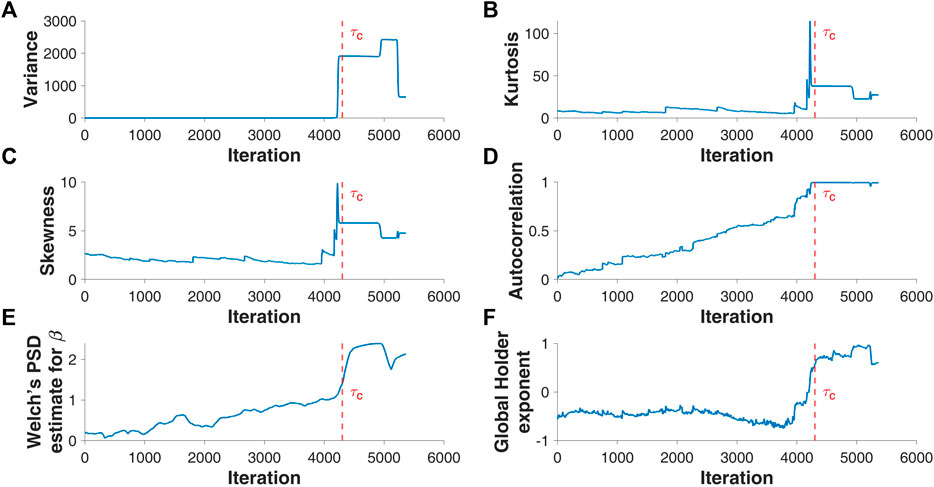
FIGURE 4. Dynamic series of variance (A), kurtosis (B), skewness (C), autocorrelation at lag-1 (D), Welch’s power spectral density estimation for power law exponent (E), and global Holder exponent (F) for the sandpile cellular automaton on the Erdos-Renyi graph with Bak-Tang-Wiesenfeld rule and pumping according to the law of discrete uniform distribution. The symbol ${\mathrm{\tau }}_{\mathrm{c}}$ indicates the critical time.

Let us now turn to the behavior of EWMs, which, perhaps with the exception of the largest Lyapunov exponent (see the paper [33]), has not yet been theoretically justified in the context of critical slowing down. We begin by discussing the results obtained for the global Holder exponent, $h$ (see Figure 4F). As the right boundary of the sliding window approaches ${\tau }_c$ we observe a decrease in $h$ followed by a sharp increase. The anticorrelated ($h<-0.5$) stochastic dynamics of the number of unstable nodes, $\left\{{\xi }_t|t\in \left[0,n-{\mathcal{w}}_0\right]\right\}$, is replaced by correlated dynamics ($h>-0.5$) at $t=4136$. When $h<-0.5$, it is most likely that large values of $\xi$ are followed by small values, and vice versa. At the dynamic mode change ($h>-0.5$) large values of $\xi$ At the dynamic mode change ($h>-0.5$), large values are followed by large values, and small values are followed by small values. The mode change at the point $t=4136$ is a precursor to the critical transition. Note that the similarity of behavior $\beta$ and $h$ is theoretically strictly justified for fractional Brownian motion, for which $\beta =2h+1$ (see the paper [26]). In spite of this, calculating $h$, in addition to the type of correlations in the dynamics of the series, we obtain an indirect estimate of the exponent $\beta$ In spite of this, calculating h, in addition to the type of correlations in the dynamics of the series, we obtain an indirect estimate of the exponent by the WTMM method.

Consider the EWMs of the reconstructed phase space $x$ [see Sequence (8)] of the dynamical series $\left\{{\xi }_t|t\in \left[k,k+{\mathcal{w}}_0\right],k\in \mathbb{N}\right\}$. Figure 5 shows the behavior of these EWMs as the automaton approaches ${\tau }_c$. At iteration $t^{\prime }=4151$, there is a sharp increase in the dimensionality of the reconstructed attractor, $M$, and a correspondingly sharp increase in the minimum number of phase variables that the dynamical system generating the dynamical series must include (see Figure 5A). Only starting from iteration $t^{\prime }$ the dynamical system generating the dynamical series exhibits complex behavior, since for complex systems $M\ge 3$ (see the paper [28]). In this case, $M$ varies from 2 to 5 for all automata we studied. Changing the topological structure of the graph and the pumping of the automaton affect only the numerical values of $t^{\prime }$. The correlation dimension of the reconstructed attractor, $D_c$, increases sharply at $t^{\prime }$, taking fractional values greater than zero at $t>t^{\prime }$ (see Figure 5B). This behavior indicates the complexity of the structure of the reconstructed attractor and an increase in the degree of chaotic complexity of the dynamical series. At $t>t^{\prime }$ the geometry of the reconstructed attractor is fractal. The approximation entropy, AppEn, increases at $t<t^{\prime }$ with a sharp decline at iteration $t=t^{\prime }$ and an increase at $t>t^{\prime }$ (see Figure 5C). Hence, in iteration $t=t^{\prime }$ there is a sharp decline in the uncertainty (irregularity and unpredictability) of the behavior of the discrete dynamic series $\left\{{\xi }_t|t\in \left[0,n-{\mathcal{w}}_0\right]\right\}$, i.e., the number of repeating patterns in such a series increases sharply. Thus, a sharp change in the behavior of measures M, $D_c$ and AppEn at $t=t^{\prime }$ is a precursor of critical transitions in automata. The behavior of the largest Lyapunov exponent, $\lambda$, due to the strong noisiness of the corresponding dynamical series is apparently not a reliable precursor of a critical transition in automata (see Figure 5D). But, in spite of the noise, it is still possible to assert that the automaton may be approaching ${\tau }_c$ by the change of value $\lambda$ from zero, at $t=2202$, to a positive value, at $t>2202$. In the latter case, the dynamics of the automaton is sensitive to small changes in the initial conditions. A reliable conclusion about the appearance of a strange attractor in the dynamics of unstable nodes of the automaton is possible only starting from iteration $t=t^{\prime }$, since $D_c$ takes fractional values and $\lambda >0$.

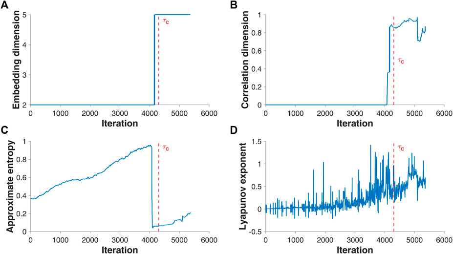
FIGURE 5. Dynamic series of embedding dimension (A), correlation dimension (B), approximate entropy (C), and Lyapunov exponent (D) for the sandpile cellular automaton on the Erdos-Renyi graph with Bak-Tang-Wiesenfeld rule and pumping according to the law of discrete uniform distribution. The symbol ${\mathrm{\tau }}_{\mathrm{c}}$ indicates the critical time.

3.2 Effectiveness of early warning measures

In the context of the definition of EWM efficiency proposed in the previous section, the efficiency of EWM for critical transitions in sandpile cellular automata depends on the magnitude of the difference between critical iteration and early warning iteration, $∆\tau ={\tau }_c-{\tau }_{ew}$, and on the number of true early warning signals, $\nu$. Thus, ${EWM}_1$ is more efficient than ${EWM}_2$ if ${∆\tau }_1>{∆\tau }_2$ and ${\nu }_1<{\nu }_2$. Figure 6 shows the magnitudes of $∆\tau$ and $\nu$ for automata. To identify an automaton, we use the abbreviations introduced in the previous section. For example, BTW-SOB-CLG-PAD stands for a sand cell automaton with Bak-Tang-Wiesenfeld rule on the Chung-Lu random graph and pumping from the Pareto distribution, which is capable of entering the SOB state.

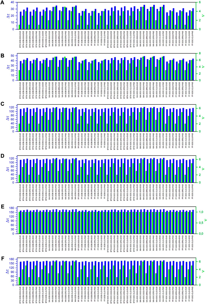
FIGURE 6. Parallel plots demonstrating the effectiveness of variance (A), kurtosis/skewness (B), autocorrelation at lag-1 (C), local Holder exponent (D), embedding/correlation dimension (E), and approximate entropy (F) as early warning measures for critical transitions in the sandpile cellular automata. The lines on the plots correspond to the difference between the early warning time and the critical time ($∆\mathrm{\tau }$), and the number of false early warnings ($\mathrm{\nu }$).

We consider the effects of the critical transition type (SOB/SOC), local rules (BTW/FF/MA), pumping distribution (DUD/EXD/PAD) and topological graph structure (SGG/ERG/CLG) on the EWM efficiency. It is found that the influence features described below are satisfied for all studied EWMs, as demonstrated by Figure 6. For two automata with the same rules, pumping and graph structures, the EWM for the SOC automaton is more efficient than the corresponding EWM for the SOB automaton, since ${∆\tau }_{SOB}<{∆\tau }_{SOC}$ and ${\nu }_{SOB}={\nu }_{SOC}$. Increasing the degree of internal (defined by local rules) and external (defined by the mean and variance of the pumping distributions) stochasticity leads to higher efficiency in terms of early warning time. Indeed, for two automata with the same critical transition types, pumping and graph structures, $∆\tau$ measures are in the relationship ${∆\tau }_{BTW}<{∆\tau }_{MA}$. Also, the inequalities ${∆\tau }_{DUD}<{∆\tau }_{EXD}<{∆\tau }_{PAD}$ for EWMs automata with different pumping distributions are satisfied for other identical features of automata functioning. Even so, increasing the degree of stochasticity of internal and external pumping leads to a decrease in the EWMs in terms of the number of true early warning signals, since ${\nu }_{BTW}<{\nu }_{MA}$ and ${\nu }_{DUD}<{\nu }_{EXD}<{\nu }_{PAD}$. Finally, changing the topological structure of the automaton graph does not affect the efficiency of EWMs under other identical features of its functioning.

To conclude this section, let us consider which of the studied EWMs are the most efficient independent of the type of critical transition, rules, pumping and automata graph structure. The measures determined by the features of the reconstructed phase space structure, such as embedding dimension, correlation dimension and approximation entropy, are effective by early warning time. Apparently, this is due to the fact that the phase space structure is most sensitive to the approximation of a number of unstable nodes of the automaton to ${\tau }_c$. Also these measures, along with dispersion, autocorrelation at lag-1 and $h$ are effective on the number of true early warning signals, with, in contrast, dispersion being the least effective EWM on early warning time. The power-law scaling exponent, $\beta$, and the largest Lyapunov exponent, $\lambda$, are not EWMs at all, so their $∆\tau$ and $\nu$ we have not presented them in Figure 6. The behavior of the measure $\lambda$ is characterized by a large number of false signals, i.e., a large number of $\nu$. This is apparently due to the insufficient width of the sliding window to adequately estimate this measure using Rosenstein’s algorithm. The numerical values taken by the measure $\beta$ in the left neighborhood of the point ${\tau }_c$, do not correspond to the values characteristic of the redness effect ($\beta =2$) at the critical slowing down of the automaton. This discrepancy is due to the inadequacy of Welch’s PSD estimate for $\beta$, since the behavior of the associated with $\beta$ measure $h$, computed by the WTMM method predicts the critical slowing down of the automaton in the left neighborhood of the point ${\tau }_c$. But, recall, that the measure $h$ is not efficient in terms of early warning time.

Thus, only the behavior of EWMs based on estimates of embedding dimension, correlation dimension and approximation entropy, in the left neighborhood of the point ${\tau }_c$ is an effective precursor to the critical transition of sand cellular automata. Only these measures have the largest $∆\tau$ and the smallest $\nu$ of all the measures studied.

4 Conclusion

Embedding dimension, correlation dimension and approximation entropy as effective EWMs can be used in real-time early-warning systems of critical transitions in real systems if its structure is analogous to that of a sand cellular automaton, i.e., the systems are isomorphic. In the context of systems theory [34], the analogy of systems structures is determined by the analogy of functioning of elements and connections between elements of systems. For example, such real systems are a segment of the online social network Twitter and a segment of the stock exchange generating dynamic series in real time. By the term “segment” we denote a set of network users connected by discussion of some topic or some event. For a stock exchange, it is a set of traders involved in buying/selling some security.

Figure 7 demonstrates the formation of chains of retweets in a segment, starting from the pumping of tweets into the network segment (tweet is shown by a red lightning bolt in Figure 7A) to the complete relaxation of the segment (see Figure 7D). The presented process corresponds to some iteration of the automaton’s self-organization process. The nodes of the graph correspond to the users of the segment, the edges of the graph determine the existence of interactions between these users. If two nodes (segment users) are connected by an edge, then one of the segment users is a subscriber of the other, and, accordingly, retweet transmission/acceptance along the edge is possible. Local retweet propagation is shown by the red dashed arrow. Each network user can be either in an active state (red nodes of the graph in Figure 7 corresponding to unstable nodes), in which it is ready to send retweets to its subscribers, or in a passive state (green nodes of the graph in Figure 7 corresponding to stable nodes), in which it is not ready to send retweets for some reason. Sending retweets to subscribers corresponds to the crumbling of an unstable node of the automaton. If some user of a segment that is in the passive state receives a tweet, that causes it to move to the active state (see Figure 7A). This event (pumping) triggers a chain of retweets in the segment, initiated by this user. This user then sends retweets to its followers, and let us assume that as a result of this retweet propagation, they move to the active state (see Figure 7B). The process of moving from passive to active state, and vice versa, continues (see Figure 7C) until the segment consisting of only passive users is completely relaxed (see Figure 7D). The next iteration also starts by pumping tweets from some users in the segment and leads to chains of retweets in the segment. Starting at some iteration (${\tau }_c$), the segment self-organizes into a critical state characterized by an avalanche-like spread of retweets. The number of unstable nodes of the automaton, $\left\{{\xi }_t\right\}$ ($t$ is the number of iterations) is analogous to the number of users of the segment that initiate retweet chains in it. If we consider the stock market, comprising bonds and derivatives, as a group of interconnected subsets, each with the potential to self-organize into a bistable or critical state, they can be modeled similarly to sand piles using the logic of the spread of information in the market through avalanches. In this instance, traders serve as nodes and their transactions denote edges in the graph. First, a trader initiates a significant deal with other market participants. As others become aware of this information, they make their independent decisions. If the information is impactful, traders are inclined to make deals that would increase the amount of available information in the market. This mechanism will persist in the bistable state, if the number of deals decreases as the systems begin to relax, or in the critical state, if this segment of the market becomes much more popular among traders on a regular basis.

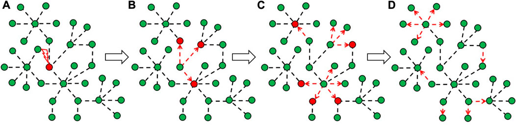
FIGURE 7. One of the possible schemes for spreading retweets on Twitter segment.

The proposed definition of effective EWMs can be used to find new effective EWMs, such as multifractal measures (e.g., see the paper [6]) and measures based on recurrences (e.g., see the paper [35]), which exhibit sharp changes when approaching ${\tau }_c$. For this reason, our approach did not allow us to assign the largest Lyapunov exponent, which is characterized by a sign change in the neighborhood of ${\tau }_c$, to the set of efficient EWMs. Perhaps another reason for the inefficiency of the largest Lyapunov exponent is that the window width (the amount of sampled data) is insufficient to obtain an adequate estimate of the exponent. In real systems the window width can be increased, for example, as a result of transition from daily data to minute data on the number of purchase/sale transactions of a security. When selecting the initial window, it is fundamentally important that it does not include ${\tau }_c$. Otherwise, a critical transition in a real system will start before the process of its early detection has been initiated.

The used rules, topological structures of graphs, and pumping of sand cellular automata allowed us to study the efficiency of EWMs for bifurcation-induced tipping. But, this type of tipping is not limited to the study of the effectiveness of the measures, because by a suitable choice of local rules and pumping it is possible to observe noise-induced and rate-induced tipping in sand cell automata (e.g., see the paper [36]).

Data availability statement

The raw data supporting the conclusion of this article will be made available by the authors, without undue reservation.

Author contributions

AD: Conceptualization, Formal Analysis, Investigation, Methodology, Validation, Writing–original draft, Writing–review and editing. AL: Conceptualization, Formal Analysis, Software, Supervision, Validation, Visualization, Writing–original draft, Writing–review and editing. VK: Conceptualization, Data curation, Formal Analysis, Funding acquisition, Project administration, Resources, Visualization, Writing–review and editing. VD: Conceptualization, Data curation, Funding acquisition, Investigation, Project administration, Supervision, Validation, Visualization, Writing–original draft.

Funding

The author(s) declare financial support was received for the research, authorship, and/or publication of this article. The work is an output of a research project implemented as part of the Basic Research Program at the National Research University Higher School of Economics (HSE University).

Conflict of interest

The authors declare that the research was conducted in the absence of any commercial or financial relationships that could be construed as a potential conflict of interest.

The reviewer VP declared a shared affiliation with the authors to the handling editor at the time of review.

Publisher’s note

All claims expressed in this article are solely those of the authors and do not necessarily represent those of their affiliated organizations, or those of the publisher, the editors and the reviewers. Any product that may be evaluated in this article, or claim that may be made by its manufacturer, is not guaranteed or endorsed by the publisher.

References

1. Bak P, Tang C, Wiesenfeld K. Self-organized criticality: An explanation of the 1/f noise. Phys Rev Lett (1987) 59:381–4. doi:10.1103/PhysRevLett.59.381
2. di Santo S, Burioni R, Vezzani A, Muñoz MA. Self-organized bistability associated with first-order phase transitions. Phys Rev Lett (2016) 116:240601. doi:10.1103/PhysRevLett.116.240601
3. Buendia V, di Santo S, Bonachela JA, Muñoz MA. Feedback mechanisms for self-organization to the edge of a phase transition. Front Phys (2020) 8:1–17. doi:10.3389/fphy.2020.00333
4. Tebaldi C. Self-organized criticality in economic fluctuations: The age of maturity. Front Phys (2021) 8:616408. doi:10.3389/fphy.2020.616408
5. Stanley H, Amaral LAN, Buldyrev SV, Gopikrishnan P, Plerou V, Salinger MA. Self-organized complexity in economics and finance. PNAS (2002) 99:2561–5. doi:10.1073/pnas.022582899
6. Dmitriev A, Lebedev A, Kornilov V, Dmitriev V. Multifractal early warning signals about sudden changes in the stock exchange states. Complexity (2022) 2022:1–10. doi:10.1155/2022/8177307
7. Tadic D, Mitrović Dankulov M, Melnik R. Evolving cycles and self-organised criticality in social dynamics. Chaos, Solitons and Fractals (2023) 171:113459. doi:10.1016/j.chaos.2023.113459
8. Tadic B, Melnik R. Self-organised critical dynamics as a key to fundamental features of complexity in physical, biological, and social networks. Dynamics (2021) 1:181–97. doi:10.3390/dynamics1020011
9. Zhukov D. How the theory of self-organized criticality explains punctuated equilibrium in social systems. Methodological Innov (2022) 15:163–77. doi:10.1177/20597991221100427
10. Odagaki T. Self-organized wavy infection curve of COVID-19. Sci Rep (2012) 11:1936. doi:10.1038/s41598-021-81521-z
11. Pruessner G, Chapman SC, Crosby NB, Jensen HJ. 25 Years of self-organized criticality: Concepts and controversies. Space Sci Rev (2016) 198:3–44. doi:10.1007/s11214-015-0155-x
12. Plenz D, Ribeiro TL, Miller SR, Kells PA, Vakili A, Capek EL. Self-organized criticality in the brain. Front Phys (2021) 9:1–23. doi:10.3389/fphy.2021.639389
13. Jarai A. The sandpile cellular automaton. In: PY Louis, and F Nardi, editors. Probabilistic cellular automata. Emergence, complexity and computation (2018). 27. doi:10.1007/978-3-319-65558-1_6
14. Scheffer M, Bascompte J, Brock WA, Brovkin V, Carpenter SR, Dakos V, et al. Early-warning signals for critical transitions. Nature (2009) 461:53–9. doi:10.1038/nature08227
15. George S, Kachhara S, Ambika G. Early warning signals for critical transitions in complex systems. Physica Scripta (2023) 98:072002. doi:10.1088/1402-4896/acde20
16. Clarke J, Huntingford C, Ritchie PDL, Cox PM. Seeking more robust early warning signals for climate tipping points: The ratio of spectra method (ROSA). Environ Res Lett (2023) 18:035006. doi:10.1088/1748-9326/acbc8d
17. Proverbio D, Kemp F, Magni S, Gonçalves J. Performance of early warning signals for disease re-emergence: A case study on COVID-19 data. Plos Comput Biol (2022) 18:e1009958. doi:10.1371/journal.pcbi.1009958
18. Huang Y, Saleur H, Sammis C, Sornette D. Precursors, aftershocks, criticality and self-organized criticality. Europhysics Lett (1998) 41:43–8. doi:10.1209/epl/i1998-00113-x
19. Zhao L, Li W, Yang C, Han J, Su Z, Zou Y. Multifractality and network analysis of phase transition. PLoS ONE (2017) 12:e0170467. doi:10.1371/journal.pone.0170467
20. Lade S, Gross T. Early warning signals for critical transitions: A generalized modeling approach. Plos Comput Biol (2012) 8:e1002360. doi:10.1371/journal.pcbi.1002360
21. Tang Y, Zhu X, He C, Hu J, Fan J. Critical slowing down theory provides early warning signals for sandstone failure. Front Earth Sci (2022) 10:1–14. doi:10.3389/feart.2022.934498
22. Shaposnikov K. Random graph models and their application to twitter network analysis. In: Proceedings of the Fourth Workshop on Computer Modelling in Decision Making; 14-15 November 2019; Saratov, Russia (2019). p. 2589–4900.
23. Manna S. Two-state model of self-organized criticality. J Phys A (1991) 24:L363–9. doi:10.1088/0305-4470/24/7/009
24. Feder Y, Feder J. Self-organized criticality in a stick-slip process. Phys Rev Lett (1991) 66:2669–72. doi:10.1103/PhysRevLett.66.2669
25. Stoica P, Randolph M. Randolph M. Spectral analysis of signals. Upper Saddle River. NJ: Prentice Hall (2005).
26. Li M. Fractal time series - a tutorial review. Math Probl Eng (2010) 2010:1–26. doi:10.1155/2010/157264
27. Mallat S, Hwang W. Singularity detection and processing with wavelets. IEEE Trans Inform Theor (1992) 38:617–43. doi:10.1109/18.119727
29. Hegger R, Kantz H. Improved false nearest neighbor method to detect determinism in time series data. Phys Rev E (1999) 60:4970–3. doi:10.1103/PhysRevE.60.4970
30. Wallot S, Mønster D. Calculation of average mutual information (AMI) and false-nearest neighbors (FNN) for the estimation of embedding parameters of multidimensional time series in Matlab. Front Psychol (2018) 9:1–10. doi:10.3389/fpsyg.2018.01679
31. Rosenstein M, Collins JJ, De Luca CJ. A practical method for calculating largest Lyapunov exponents from small data sets. Physica D (1993) 65:117–34. doi:10.1016/0167-2789(93)90009-P
32. Tan J. Critical slowing down associated with regime shifts in the US housing market. Eur Phys J B (2014) 87:38. doi:10.1140/epjb/e2014-41038-1
33. Das M, Green JR. Critical fluctuations and slowing down of chaos. Nat Commun (2019) 10:2155. doi:10.1038/s41467-019-10040-3
34. Skyttner L. General systems theory: Problems, perspectives, practice. Singapore: World Scientific (2006).
35. Hasselman F. Early warning signals in phase space: Geometric resilience loss indicators from multiplex cumulative recurrence networks. Front Physiol (2022) 13:859127–18. doi:10.3389/fphys.2022.859127
Keywords: early warning signals, critical transition, self-organized criticality, self-organized bistability, sandpile cellular automata, wavelet transform, phase space reconstruction, early warning systems
Citation: Dmitriev A, Lebedev A, Kornilov V and Dmitriev V (2023) Effective precursors for self-organization of complex systems into a critical state based on dynamic series data. Front. Phys. 11:1274685. doi: 10.3389/fphy.2023.1274685
Received: 08 August 2023; Accepted: 06 September 2023;
Published: 22 September 2023.
Edited by:
Ming Li, Zhejiang University, ChinaReviewed by:
Ming Tang, East China Normal University, ChinaChanggui Gu, University of Shanghai for Science and Technology, China
Viktor Popov, National Research University Higher School of Economics, Russia
Copyright © 2023 Dmitriev, Lebedev, Kornilov and Dmitriev. This is an open-access article distributed under the terms of the Creative Commons Attribution License (CC BY). The use, distribution or reproduction in other forums is permitted, provided the original author(s) and the copyright owner(s) are credited and that the original publication in this journal is cited, in accordance with accepted academic practice. No use, distribution or reproduction is permitted which does not comply with these terms.
*Correspondence: Andrey Dmitriev, a.dmitriev@hse.ru