Metapopulation Network Models for Understanding, Predicting, and Managing the Coronavirus Disease COVID-19

1. Introduction

Predicting the spread of COVID-19 is critical to public health decision making, including decisions to relax mitigation measures in different communities. Data on the number of individuals testing positive for the novel coronavirus in every county of the USA is updated continuously and used to inform mathematical models for predicting how the pandemic will evolve. A COVID-19 forecasting algorithm based on newly daily infections was recently proposed [1]. The novelty of the virus and the current lack of testing capacity for the general population add to the challenges of the task, and can explain the wide variability seen in model predictions.

The use of mathematical models to study the dynamics of infectious diseases has a long history. Classical population models [2] have been used extensively to study the spread of epidemics for nearly a century. The models commonly assume that the populations in the various compartments are homogenous, in the sense that all individuals behave similarly, and well-mixed, i.e., transmission affects all individuals in a compartment at once [3–5]. These models can be useful to understand the overall dynamics of an epidemic and provide fairly realistic predictions for a homogeneous population, but may not have enough resolution when the population consists of communities with different socio-urban characteristics or demographics. The need for models that account for the diverse modes of social interaction within each community has been acknowledged for a long time, and the mobility pattern among communities is particularly crucial when trying to forecast the effects of different measures to contain and control the transmission. The concept of metapopulation, intended as a group of spatially separated populations that have some kind of interaction, was initially introduced in a study of insect pests [6] and later used in conjunction with networks to introduce a spatial dimension in modeling transmission of disease. The network aspect comes from the transfer of individuals among the nodes, and the level of communication between any pair of nodes is determined by the mobility network [7]. Information about the mobility network can be gleaned from census data, cell phone data, or from domestic or international air travel schedules, as relevant for the spatial scale of the model.

In Wang and Li [8], the authors advocate network metapopulation models for describing the spread of SARS and the outbreaks of A(H1N1) influenza, and A(N7H7), known as avian flu. The common feature of these three epidemics was the speed at which their incidence spread over a wide geographic range: in 2003, before being contained, SARS-CoV spread from Hong Kong to over 30 countries on 4 continents, and in 2009 A(H1N1) spread in 3–4 months to 214 countries and overseas territories or communities. By comparison, SARS-CoV-2 has spread to nearly every country in the world in less than 6 months, following a pattern similar to that of a wild fire. Human recurrent commuting data in metapopulation network models have been used to study changes in contagion processes [9–11]. For a comparison of large scale computational approaches to epidemic modeling, in particular agent-based approach vs. structured metapopulation models, see Ajelli et al. [12]. Changes in human mobility pattern are often enforced at the outbreak of an epidemic to keep it localized to the original hotspot, however the effectiveness of travel bans for containing a pandemic has been questioned [13–16]. To contain the COVID-19 pandemic, measures to control human mobility have varied from the ban of most international flights from affected areas, to the near full suppression of traffic between communities in regions with high prevalence of infections. In addition, changes in mobility have occurred in reaction to the spread of epidemics [17–19]. As reported in Poletti et al. [20], the changing perception of risk did indeed affect the 2009 H1N1 pandemic dynamics.

A commonly observed pattern of COVID-19 spread is that once the virus enters densely populated communities with no mitigation measures in place, the disease is likely to flare up rapidly, infecting a large number of individuals in a short amount of time, with the risk of overwhelming the local health system, as has been the case in the region around Milan, Italy and in New York City. Not surprisingly, the first COVID-19 infection in many countries has been recorded in cities that, being major economic hubs or tourist centers, with significant contacts with previously infected areas. Contact between communities is responsible for the spread of COVID-19, and patterns of contact need to be taken into consideration when predicting where the next hot spots are likely to emerge.

It has been established that the SARS-CoV-2 is transmitted through respiratory droplets and that symptoms go from non-existent to life-threatening. The range of clinical presentation has also been wide and includes constitutional, respiratory, gastrointestinal, dermatologic, and musculoskeletal signs and symptoms. Unlike the case for SARS, where virus transmission appears to have occurred primarily after the emergence of symptoms, there is evidence that viral shedding of SARS-CoV-2 occurs, and may even peak, during the few days just prior to symptom onset [21]. The potential for pre- or oligosymptomatic transmission was supported early in the pandemic by the report of cases with mild symptoms [22], and significant spread of the infection by asymptomatic cases became a concern from the start of the outbreak. The recommendations to maintain at least 6 feet of social distance from other individuals and to wear face masks in public places are addressing the concerns about asymptomatic infections, as are state-level bans on large gatherings. As of May 22, 2020, the Center for Disease Control and Prevention (CDC) in its Modeling COVID-19 Planning Scenarios stated that, based on the available data, asymptomatic cases constitute approximately 35% of all infections, and that the absence of symptoms does not reduce infectiousness. These values are higher than earlier estimates [23] of 14% of total cases, assumed to be nearly half as infectious as reported symptomatic ones.

Classical mathematical models for the spread of epidemics subdivide the population into cohorts of susceptible (S), infected (I), and Recovered (R) individuals, (classical SIR models of [2]), with the possible addition of a fourth Exposed (E) cohort, accounting for the incubation time before infection onset (SEIR models). Both SIR and SEIR models assume that the underlying population and the subpopulations within each compartment are well-mixed, a necessary condition for the mean field description to be accurate. In the case of COVID-19, the lack of immunity of the population due to the novelty of the virus and the ease of transmission through respiratory droplets make its spread very sensitive to the type and frequency of contacts among individuals in the community. Such contacts may depend strongly on population density; therefore, to reduce violation of the mean field assumption, communities with differing population densities should be modeled separately.

In addition to different contact rates, traffic between communities also plays an important role in the spread of the pandemic, as individuals arriving from an area with a large number of infections act as potential vectors for the virus previously uninfected communities. Although homogenized SIR and SEIR models are not suited to account for these important aspects of the spread of COVID-19, they can form the fundamental units of a metapopulation model of interconnected communities, with separate sets of parameters accounting for community-specific settings. In addition to providing a more realistic explanation of the geographic pattern of spread, metapopulation models can also be used to test which changes in commuting patterns are more likely to keep the pandemic under control.

Finally, it is important that COVID-19 models acknowledge the time dependency of model parameters, as the pathogen may mutate and the number and type of contacts change in response both to mitigation measures imposed and to population's awareness of risks, and ongoing adherence to public health guidance. The time course of key parameters can provide valuable insight into the spread patterns and aggressiveness of the disease, as well as into the effectiveness of various mitigation measures.

In this time when different states in the USA are debating whether relaxing mitigation strategies and travel restrictions are likely to create new hot spots in areas little affected by the pandemic, a predictive model that can be adapted to different regions can have an immediate applicability. In response to these needs, the aim of this study is to adopt a new network model of COVID-19 spread to understand the dynamics of the pandemic in a network of 18 counties in the region of Northeast Ohio around Cleveland, and a network of 19 counties in Southeast Michigan around Detroit. The computational model within each county, referred to as SE(A)IR, includes an asymptomatic, infected, and infectious cohort to account for the transmission by asymptomatic individuals, and it addresses all of the points discussed above: The model parameters may be variable in time, and up to date Bayesian computational tools are used to inform the model on a daily basis regarding the progression of the epidemic, providing also an estimate of the uncertainties of the estimates. The metapopulation model uses census data to track population density and the movement of individuals between communities [24]. Importantly, the model gives an estimate of the size of the asymptomatic cohort based on the observed new infection count. Finally, to avoid introducing intractable or uninterpretable parameters that could limit usability and interpretability, the basic model is as simple as possible without overlooking some fundamental characteristics of COVID-19. The output comprises interpretable quantities that can be immediately communicated to public health and health system decision makers, and allow a comparison with existing model predictions. The computational framework can be shown to reproduce within reasonable uncertainty the observed timeline of spread between the communities included in this study; and the predictive skills over relatively short time windows, up to a few weeks, can be demonstrated. The network model predictions suggest that while human mobility is the pathway for the spreading of the virus, reducing traffic between the communities by itself is not an effective way to contain the epidemic. Furthermore, the simulations show that local social distancing triggered by case prevalence is essentially as efficient mitigation measure as a state-wide blanket social distancing strategy.

2. Materials and Methods

2.1. Predictive Models of COVID-19

In the absence of data from previous outbreaks, mathematical and statistical models, e.g., CHIME: COVID-19 Hospital Impact Model for Epidemics, and the IHME models by C. Murray and collaborators, are the main tools to predict how the COVID-19 outbreak will progress, including estimates of how many patients will need to be hospitalized, the expected number of admissions to ICU and the type of resources that the health systems should have ready. In the current active epidemic outbreak, computational methods capable of dynamic model updating as data are gathered are of key importance.

2.2. A SE(A)IR Model of COVID-19 Spread

In epidemiology, classical compartment models such as SIR and SEIR [2] have been used successfully to model epidemics for nearly a century. In the case of COVID-19, there is evidence of exposed individuals shedding the virus already a few days before developing any symptoms. In fact, according to some recent laboratory tests, the amount of virus released is largest right before the onset of the symptoms, and over the next few days it starts to decay [21, 25]. Moreover, the presence of antibodies in individuals who did not report any symptoms of COVID-19, points toward a presence of a potentially large number of asymptomatic infectious individuals, who spread the virus without being detected [26, 27], in particular when testing is reserved for individual with clear symptoms. Furthermore, if the I cohort in the SEIR model comprises symptomatic infected and infectious individuals who have tested positive for COVID-19, it is reasonable to assume that most of them will be in some form of isolation, hence with limited contribution to the spreading of the infection.

To account for the possibility that the asymptomatic/oligosymptomatic infectious pool is mostly responsible for the spread of the infection, we introduce a cohort A of infected, infectious, and asymptomatic individuals in the SEIR model, and assume that this cohort is principally responsible for new infections. At the time of writing this article, the available data comprise almost exclusively the number of reported symptomatic daily new infections, which does not allow inference on the size of the asymptomatic cohort. To avoid introducing ill-defined assumptions about the prevalence of symptoms, we combine the E and the A compartments into a single asymptomatic compartment E(A). As demonstrated in Calvetti et al. [28], this allows us to directly estimate the E(A) cohort size from available data. While losing some of the time resolution of the model, this approximation gains indirect observability that is essential in tracking the virus spread. To underline this interpretative difference, and the embedding of the asymptomatic A cohort in E, we refer to the model as SE(A)IR model. Figure 1 shows a schematic compartment diagram and the governing equations, illustrating the modification to the standard SEIR model to account for asymptomatic infectious individuals.

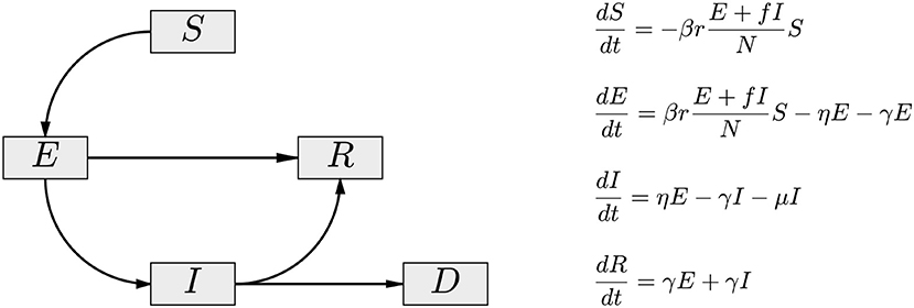
Figure 1. The compartment diagram of the SE(A)IR model. Compared to the standard SEIR model, the flux E → R has been added, and the non-linear interaction term is modified by the replacement I → E + fI. Here, 0 < f < 1 accounts for the fact that diagnosed symptomatic individuals are in partial isolation, contributing less to the infection than the asymptomatic individuals (A) embedded in the exposed cohort E of the model. In the presented calculations, the value f = 0.1 is used.

When used for interpretation of real data, the classical compartment models usually suffer from two limitations: (i) The model parameters are constant in time, while the population interaction is a dynamic process, and (ii) the models operate under the hypothesis that the population is well-mixed, while in reality the data are an aggregate of underlying sub-populations with a complex interaction structure. Below is the description of our contribution and findings, with an emphasis on two particular cases, population models of Northeastern Ohio and Southeastern Michigan in the period from early March 2020 to early May 2020.

2.3. Bayesian Estimation of the SE(A)IR Parameters

The governing equations of the SE(A)IR model (see Figure 1) depend on a number of parameters reflecting the characteristics of the epidemic: more precisely, β>0 is the infectivity rate, or probability of contagion, r the number of contacts per day of infectious and susceptible cohorts, η = 1/T_inc the incubation rate in days, the reciprocal to the expected time of incubation of the disease, γ = 1/T_rec the expected recovery rate, T_rec being the expected number of recovery days, and μ the mortality rate. The latter three parameters (incubation, recovery, and mortality rates) are strongly pathogen dependent and to some extent sensitive to factors like demographics and co-morbidities, but for modeling purposes, they can be considered independent of time. Arguably, the most important parameter is the product βr, controlling the rate at which susceptible individuals are infected. While the value of β depends mostly on the infectivity power of the virus, the factor r, accounting for the frequency of contacts between infectious and susceptible individuals, may change significantly with population-level behavior, whether voluntary or enforced. In fact, the effectiveness of the measures can be directly monitored by estimating this quantity, and in particular, the time dependency of it.

In the methodology that we propose, for each subpopulation of individual counties, the product rβ is assumed to be time dependent, and is estimated using a Bayesian filtering technique known as particle filtering (PF), discussed by Liu and West [29] and Arnold et al. [30–32]. In PF, thousands of realizations (particles) of the model, each consisting of its own set of parameter values and cohort sizes, simulate the day-by-day propagation of the epidemic. Each day, the predictions of the particles for the next day are computed and compared to the new data, and particles whose predictions are in better agreement with the data are retained and replicated, while particles which explain the data less well are discarded. After this “survival of the fittest” step, the replicated particles are proliferated through a randomization, guaranteeing a rich variability of the particle cloud to account for the variations in the next time step. Since the effects of changing mitigation strategies are reflected in the value of rβ, this quantity is updated daily, thus providing a time series for each particle. As pointed out, unlike in standard epidemiologic model, we do not assume that the quantity is constant. In our current model, the parameter rβ is estimated by particle filtering while the values of η and γ are kept fixed. A systematic study of the sensitivity of the results to the values of η and γ, reported in Calvetti et al. [28] indicate that in general, while changes in the incubation and recovery time can be seen in the estimate of the reproduction number R₀, the predicted number of new infections and the ratio of asymptomatic to symptomatic cases remains essentially unaltered as the parameters vary within a range. The PF model, informed with the daily new number of confirmed cases, estimates an approximate 0.5 ratio of asymptomatic to symptomatic infectious cases over a wide range of different communities, which is in full agreement with the CDC suggestion on May 26, 2020 [33] that approximately 35% of the infectious individual do not develop symptoms. However, according to the model, most infections are due to the asymptomatic cohort. The estimation of the model parameters from daily counts rather than from the cumulative number of infections has been shown to reduce the bias as well as to lead to better forecasts and uncertainty quantification [34].

The data used for estimating the parameters and the cohort sizes comprise the daily count of confirmed new, presumed symptomatic, infections I, while no direct data of the cohort size of asymptomatic and exposed E(A) is available. Therefore, estimating the time evolution of the state vector (S, E(A), I, R) together with the parameter rβ provides direct information about the number of asymptomatic individuals. One of the key parameters of interest to us is the ratio ρ = E(A)/I. It turns out that this ratio tends toward a time dependent equilibrium value, ρ → ρ^*, as the infection progresses, allowing us to define in a very natural way an equivalent of the basic reproduction number R₀ of the SE(A)IR model. In the classical SIR model, the basic reproduction number is defined as a dimensionless quantity R₀ = (rβ)/(γ + μ), and a wealth of literature exists for generalization and estimation of R₀ for more complex models, see, [35–40], as well as some critical views on its usefulness, as in Li et al. [41]. For the current model,

and the equilibrium value ρ^* can be estimated in a straightforward manner if an estimate for the product βr is available, see Figure 5 for further clarification of the symbols. The novel R₀, which depends on rβ and therefore on time, has a similar role in the model as it has in the SIR model, that is, the infections spreads only if R₀ > 1, thus giving a useful summary for policy makers of the success of the mitigation efforts. Conversely, the above formula provides a means of estimating ρ^* and thereby the size of the asymptomatic cohort if R₀ has been estimated from the data, e.g., by fitting an exponential to the cumulative data of infected individuals.

One of the advantages of the particle filtering approach over data fitting approaches is that it allows us to assess the model uncertainties. At each time step, thousands of realizations of every quantity of interest are computed, and of those realizations, one can generate histograms, posterior intervals of different degrees of belief, expectations, and median values. In particular, the time traces of the quantities are not summarized in a single curve but are presented as posterior envelopes, or credible envelopes of given level of belief. Moreover, the particles can be propagated in the future to provide predictive envelopes of future data.

2.4. Metapopulation Network Models of COVID-19 Spread

The travel of individuals carrying the virus between communities is the main engine for spreading pandemics, both at the local and global level. The pattern followed by the spread of COVID-19, similar to that of the 1918 influenza, indicates that at first, the flair-up occurs typically in larger cities with a high population density, then moving to smaller, more rural communities when the number of new infected in the cities has already decreased. The predictions of mathematical models for the COVID-19 spread in a network of diverse connected communities can be used to understand where the next hot spots are likely to occur, and to design mitigation measures to keep the epidemic from overwhelming the healthcare system.

As pointed out in the literature [8], well-mixed compartment models have a limited capability for explaining the dynamics of the epidemics in large heterogenous populations, as they ignore the local dynamics depending on population density, segregation of diverse groups, and geographic separation of communities. In line with the county by county reporting of infections, metapopulation network models (MNM) are an appropriate tool to address the population inhomogeneity. To model the effect of daily commuter traffic on COVID-19 spread, an MNM can be designed as a directed graph where the counties constitute the nodes and the weights of the directed edges are proportional to the number of commuters between pairs of counties. Although the epidemic within each county can be described locally with a SE(A)IR model, the model cohorts need to be adjusted to reflect the movement of individuals between counties, thus affecting the infection dynamics.

The interaction between the subpopulations can be built in the interaction term of the SE(A)IR model, see Figure 2 for an explanation. Infections in a given node arise through contacts between susceptible residents of the node with infectious individuals in target nodes of the commuting traffic, the domiciliary node included, plus the infections that happen in the home community, e.g., during weekends and evenings. These two infection mechanisms are included in the model with weights proportional to the average time spent in work/leisure outside the home community and the time spent at home. Each community has its own characteristic number r_j of daily contacts, the number being presumably higher in densely populated urban centers than in sparsely populated rural communities with fewer interaction opportunities. The value of r_j will decrease in response to the adoption and adherence to mitigation measures that discourage group gatherings.

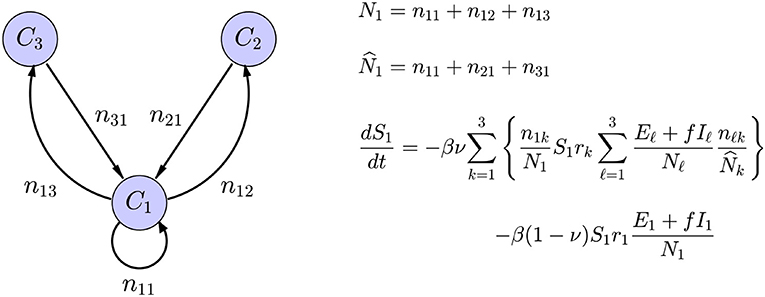
Figure 2. Schematic representation of a network model with three nodes, with only the in-links and out-links of C₁ included. The symbol n_jk indicates the number of residents of node C_j commuting to node C_k, the home community being an option, and N_k is the size of the population residing in node C_k, while ${\hat{N}}_k$ is the size of the population working in the community C_k. The average number of daily contacts in community C_k is r_k, ν is the fraction of time spent in the destination of commute, and 1 − ν is the fraction of time spent in the home community. Only the expression for the rate of change of S₁ is shown: The first term corresponds to infections through contacts of the susceptible portion S₁ of the residents in C₁ that have occurred in the commuting destinations and the second to infections in the home community.

2.5. Two Network Models: Northeast Ohio and Southeast Michigan

The methodology was tested with the daily updated infection data corresponding to 18 counties in Northeast Ohio, listed in Table S1, and with 19 counties in Southeast Michigan, see Table S2. The comparison of the two regions is of particular interest, as they both represent a population with similar cultural background and to some extent similar demographics and mixtures of dense urban areas, suburban commuter communities and rural areas. However, the mitigation measures were introduced slightly differently, and at a different stage of the epidemic.

Commuter data was procured from the Census Bureau's American Community Survey (ACS) of 2015. In the ACS, commuter data for the residents of each county was compiled that quantified the number of residents leaving the county for work in another county. The focus of this study was on the 18 county region that comprises Northeast Ohio and the 19 county region the comprises Southeast Michigan, therefore the commuting data was used for commuter traffic within these regions only. This is integrated into our model by computing n_jk from the data from the ACS of the number of people commuting from county j to county k. Commuting data for counties outside of the region of interest is not used in this model, but the region of interests were chosen to envelop the urban centers of Northeast Ohio, (e.g., Cleveland, Akron, Canton, and Youngstown) and Southeast Michigan (e.g., Detroit, Flint, Ann Arbor, and Lansing).

3. Results

Before reporting the results with the metapopulation network model, we present some of the preliminary results obtained with particle filter method for each individual county. This information captures the characteristics of the transmission within a community prior to accounting for the contribution from the mobility. A discussion of the computational details can be found in the manuscript [28].

3.1. Parameter Estimation in Individual Communities

To get a preliminary estimate of the transmission rate in each individual county, we used the particle filter with the daily new infections data from all of the 18 + 19 counties, and generated credibility envelopes for: The infection rate parameter βr, the ratio of the asymptomatic and infected cohort sizes ρ = E/I, the R₀ derived from the estimated parameter βr. Figures 3, 4 shows the outcomes for select counties.

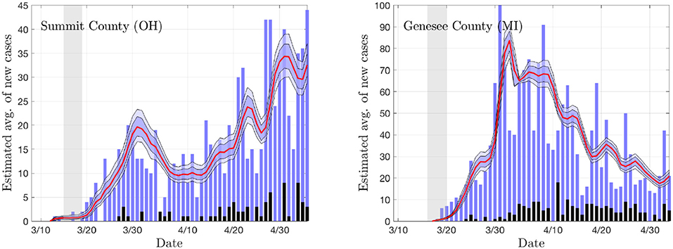
Figure 3. The daily new infection data from two counties, Summit County in Ohio (Akron) and Genesee County in Michigan (Flint). The blue envelopes represent the 50% (dark) and 75% (light) posterior model uncertainty of the expected value of new infections, and the red curve represents the median. The dark gray columns are the number of deceased (not used in the estimation). The vertical gray shading indicates the period in which the state-wide mitigation measures were adopted (Ohio: 3/15/20–3/19/20, Michigan: 3/16/20–3/23/20). The number of particles is 5 000. In the model, the new infection count is assumed to be Poisson distributed around the expected value.

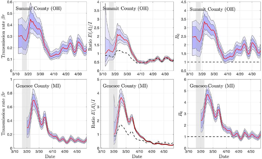
Figure 4. Sample outputs of the PF algorithm. The top row shows results based on daily new confirmed positive cases in Summit County (OH), and the second row in Genesee County (MI). In each plot, the envelopes represent the 50% (dark) and 75% (light) posterior belief. From left to right: The estimate of the rate of transmission βr, the ratio of number of asymptomatic and symptomatic individuals, and the estimated basic reproduction number R₀. In the middle column, the dashed curve represents the equilibrium value of the ratio, and in the right column, the horizontal dashed line indicates the critical value R₀ = 1. The gray vertical shading indicates the dates when the respective state started the social distancing measures. Observe that the drop in R₀ and rβ appear with a lag of about a week.

In the sample calculations, the recovery and incubation times were kept constants. The incubation and recovery times represent average approximations, the novelty of the virus leaving reliable values open to discussion [21]. Based on literature [42–44], we use T_inc = 7 days for the incubation period. For the recovery time, we use T_rec = 21 days. An analysis of how changing T_rec and T_inc affects the estimated parameter values and estimated relative sizes of the symptomatic and asymptomatic cohorts can be found in Calvetti et al. [28]. The key important parameter, the transmission rate βr, seems not to be overly sensitive to changes in the parameters, and we found that, combined with the network model, decreasing T_rec from 21 to 14 days had minimal effects on the predicted spread of the infection. Figure 5 sheds some light on how the R₀ changes if different values were used. Here, the R₀ value is plotted against the transmission rate with different combinations of the two time constants.

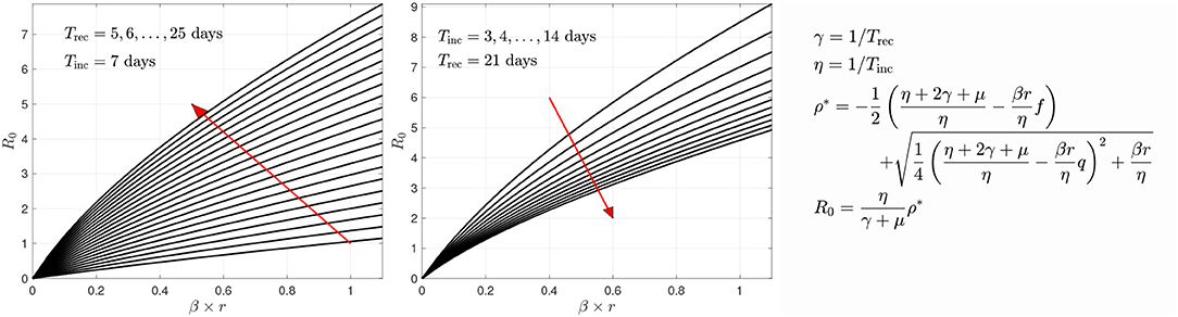
Figure 5. The variation of R₀ as a function of the transmission rate βr with respect to recovery time (left) and incubation time (right). The red arrows indicate the direction of growth of the time constants T_rec or T_inc, respectively. The derivation of the formula for R₀ is given in Calvetti et al. [28]. In the form given here, it is implicitly assumed that the infection is in its outbreak phase, and no herd immunity is present.

Figure 6 illustrates of the prediction skill of the PF method. In the figure, the last 10 days' data are left out from the PF update and the state/parameter estimation is stopped early. Consequently, the state and parameter values for each particle are propagated forward for 10 days without data-based updating, and the predicted average of new cases for each particle is calculated. These average values are used as means for a Poisson process, and random realizations of predicted new cases for each particle are computed. Finally, the predicted data are used to calculate the predictive envelopes of a given level of belief. In general, the true data may not fall in the predicted intervals, but in general, the algorithm anticipates the trend rather well. Observe that the predictions are not based on curve fitting, as the dynamics are determined by the full state vector containing components (susceptible and asymptomatic cohorts) that are not directly observed.

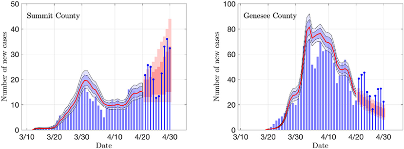
Figure 6. Examples of the prediction skill of the PF method. The PF updating is stopped 10 days before the last data, and the particles are propagated using the last update of the states as initial values, and corresponding estimates for the parameter βr. The predicted infections are drawn from Poisson distribution, and the 50 and 75% predictive intervals for the data are computed. The true data are shown as stem plots. Observe that the predicted trend corresponds well to the estimated R₀ shown in Figure 4.

3.2. Visualization of the Predictions of the Network Model

One of the central questions in the network model is how to trace the spreading of the infection between the nodes. To see if the network model is realistic, we estimate the delay of the onset of infection in the nodes after the infection is started in one of them. To validate the results with real data, the infection is initiated in the node with the first confirmed case: In Ohio, the first infection was reported on 3/9/2020 in Cuyahoga County (Cleveland) and in Michigan on 3/10/2020 in Wayne County (Detroit).

3.2.1. Reference Case

Using the estimated transmission rates for the two regions of interest, we are able to delineate differences in contact frequency r between urban and rural counties. Contact frequencies for each county were chosen to be in line with the peak estimated transmission rate, which presumably corresponds to the contact frequency before state issued stay-at-home orders were fully in place. The simulation was then initiated with one infected individual in Cuyahoga County and Wayne County, respectively, and run for 20 weeks.

Plotting the percentage of infected individuals relative to the population over a map of the counties of interest in Southeast Michigan and Northeast Ohio in Figure 7, we are able to observe the dynamics of the spread of COVID-19 infections over the two regions. For Southeast Michigan, we note the initial rise in infections in Wayne County, as well as the two neighboring, densely populated communities of Oakland County and Macomb County, which form the greater Detroit metropolitan area. As the infection spreads in the Detroit metropolitan area, surrounding counties begin to see a rise in infection. However, this spread does not correlate with physical proximity but rather with commuter traffic, as seen with Lapeer County, a sparsely populated county physically bordering Macomb County and Oakland County, however, with no interstate connection to either. Lapeer County experiences a spike in cases nearly 10 weeks after the initial infection in Wayne County. As the infection takes hold in each county, the number of the infected peaks before slowly decreasing, with differences in the relative peak values due to the differing populations of each county.

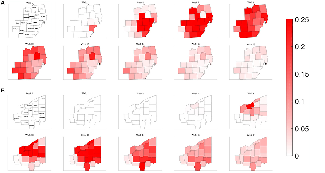
Figure 7. Map of the counties in the region of interest of (A) Southeast Michigan and (B) Northeast Ohio, where the color on the county corresponds to the fraction of the population that is infected for the reference case of section 3.2.1.

Observing the result of the Northeast Ohio simulations in Figure 8, we find that the spread of infection takes longer to fully realize in Cuyahoga County. This is in part due to the lower estimated transmission rates for the set of Ohio counties, reflecting a lower frequency of contacts. Once the infection has taken hold in Cuyahoga County, the infection then spreads to neighboring counties and grows in the urban population centers of Mahoning, Stark, and Summit counties, as well as Lake and Lorain counties, which contain suburban bedroom communities that have highways that connect to Cuyahoga. Similarly to what was observed for Southeast Michigan, we note that the number of the infected peaks quickly before subsiding at slower rate.

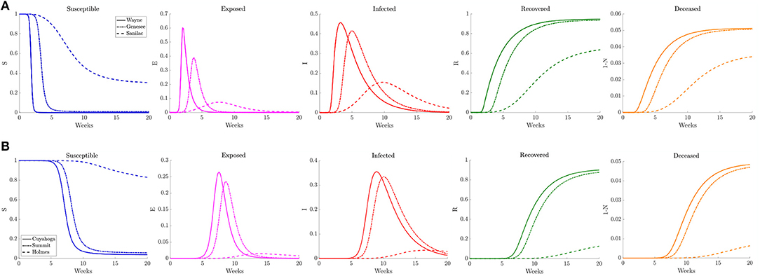
Figure 8. Plots of the relative (left to right) susceptible, exposed, infected, recovered, and deceased populations for the reduced traffic study (section 3.2.1) for (A) Wayne, Genesee, and Sanilac counties in Southeast Michigan and (B) Cuyahoga, Summit, and Holmes counties in Northeast Ohio. Note the relative scale for the y-axis.

In Figure 8 we plot the relative number of susceptible, exposed (asymptomatic), infected, deceased, and recovered population for three counties of differing population densities for both Southeast Michigan and Northeast Ohio. In Michigan the focus is on Wayne County (high density, population of 1, 257, 584), Genesee County (medium density, population of 405, 813), and Sanilac County (low density, population of 41, 170). We observe the initial sharp spike from Wayne County, followed by a spike in Genesee County. Sanilac County experiences its spike as the number of infected decreases in both Wayne and Genesee Counties. Note that the relative peak in infections is higher in Wayne County and Genesee County than Sanilac County. This highlights the role of population density and contact frequency in the propagation of the epidemic.

In Ohio, we chose to examine Cuyahoga County (high density, population of 1, 235, 072), Summit County (medium density, population of 541, 013), and Holmes County (low density, population of 43, 960), which correspond roughly to the same profile as Wayne, Genesee, and Sanilac Counties, respectively. We observe that the relative peaks in infected population are staggered, with Cuyahoga County experiencing the first spike in infections, followed soon after by Summit County, and eventually by Holmes County. We also note that the height of the peak for relative number of infections is fairly similar for both Cuyahoga and Summit Counties. That is in part due to the relatively similar contact frequency within the two counties, whereas Wayne County has a much higher contact frequency than Genesee County. Holmes County, which has lower contact rate and population, experiences a much milder peak many weeks after the peaks in the other two counties.

3.2.2. Reduced Traffic

In order the examine the role of commuting on the spread of the disease, we run a simulation reducing the number of commuters from other counties to 1% of the original amount, while keeping the contact frequency unchanged inside each county. This would be akin to nearly shutting down each county but allowing people to continue to move about in their county. Plotting the relative population of infected on the counties of each region in Figure 9, we find a similar picture to the reference case for both Southeast Michigan and Northeast Ohio, with the virus spreading initially at the source of the infection before spreading to surrounding counties. However, the speed at which the infection spreads to surrounding counties is diminished.

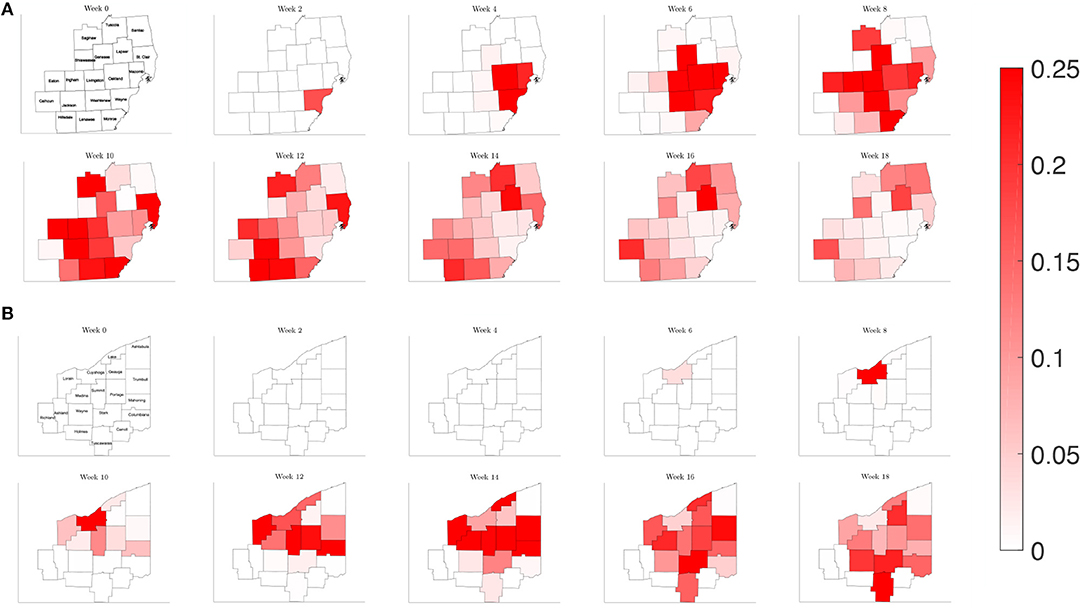
Figure 9. Map of the counties in the region of interest of (A) Southeast Michigan and (B) Northeast Ohio, where the color on the county corresponds to the fraction of the population that is infected for the reduced traffic study of section 3.2.2.

Examining the curves in Figure 10 of the different SE(A)IR compartments for the same previous three counties for each region, we find the point in time when peak infections occur for counties that are not the source of the infection to be delayed with respect to the reference case. Note that in the reference case, the nature of the network caused a 1 to 2 week delay in peak infection for Genesee and Summit Counties with respect to Wayne and Cuyahoga Counties, while in this reduced traffic scenario, the delay was more prolonged with 3 to 4 weeks difference. The overall peak of each of the curve remained similar in profile to what was observed in the reference case. This study shows that while the reduction in commuter traffic may delay the rise of infection, it does not attenuate the severity of the disease.

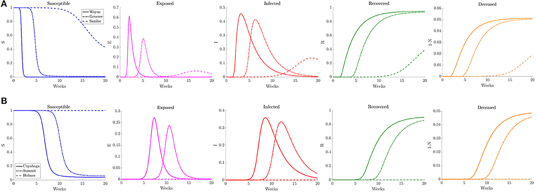
Figure 10. Plots of the relative (left to right) susceptible, exposed, infected, recovered, and deceased populations for the reduced traffic study (section 3.2.2) for (A) Wayne, Genesee, and Sanilac Counties in Southeast Michigan and (B) Cuyahoga, Summit, and Holmes Counties in Northeast Ohio. Note the relative scale for the y-axis.

3.2.3. Varying Contact Frequency

When estimating the transmission rate in the individual counties using the reported cases, we noted an initial increase before settling to a lower value. This decrease shortly follows the promulgation of stay-at-home orders in both Michigan and Ohio. To account for this, we present a simulation where the frequency of contacts is varied such that it initially has the higher value of the reference case before shifting to a lower contact frequency after 2 weeks. In Figure 11, we observe that the virus initially spreads to the three counties that constitute the core of the Detroit metropolitan region before the lower contact frequency regime begins. After the introduction of the lower contact frequency regime, the infection does not spread to other surrounding counties and is contained to the three core counties, as seen in Figure 12. In Ohio, the lower contact frequency regime occurs before the virus is able to gain a foothold in Cuyahoga County. In Figure 12, we notice a small growth in the number of infected, but not enough to result in an appreciable number of infected individuals in the Northeast Ohio region. These simulations illustrate the pivotal role of contact frequency in determining the trajectory of the disease.

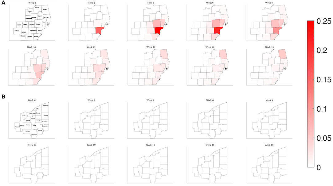
Figure 11. Map of the counties in the region of interest of (A) Southeast Michigan and (B) Northeast Ohio, where the color on the county corresponds to the fraction of the population that is infected for the varying contact frequency study of section 3.2.3.

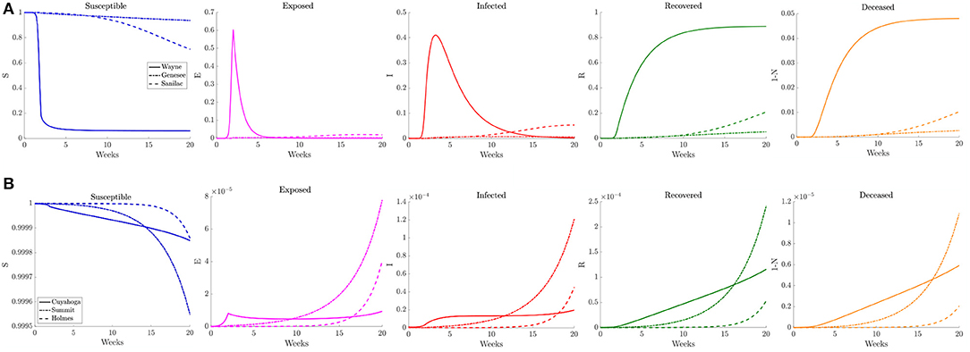
Figure 12. Plots of the relative (left to right) susceptible, exposed, infected, recovered, and deceased populations for the varying contact frequency study (section 3.2.3) for (A) Wayne, Genesee, and Sanilac Counties in Southeast Michigan and (B) Cuyahoga, Summit, and Holmes Counties in Northeast Ohio. Note the relative scale for the y-axis.

3.2.4. Physical Distancing in Response to a Trigger Case Prevalence

To illustrate how this network model can be used to evaluate public health policies, we introduce a scenario where a triggered physical distancing regimen is in effect. In this simulation, a higher contact frequency regimen is maintained within each county until the infection rate is above 100 per 100,000, at which point the county shifts to a lower contact frequency regimen. Applying this regimen to our network model, we observe in Figure 13 that the number of infected initially increases rapidly for the three counties that make up the Detroit metropolitan region, before the regimen shift occurs. This adaptive regimen yields lower overall rates of infection in all three counties and keeps the infection from spreading throughout the region without restricting mobility in any way. In Figure 14, we find that while the infection does grow slightly, the switch to a lower contact frequency causes a flattening of the curve. In the analogous simulation for Northeast Ohio, the infection increases in Cuyahoga County and spreads to other counties (Figure 13), but the overall number of infected people at peak is much lower than for the reference case and reduced traffic study.

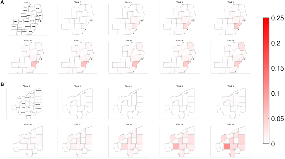
Figure 13. Map of the counties in the region of interest of (A) Southeast Michigan and (B) Northeast Ohio, where the color on the county corresponds to the fraction of the population that is infected for the triggered physical distancing regimen scenario of section 3.2.4.

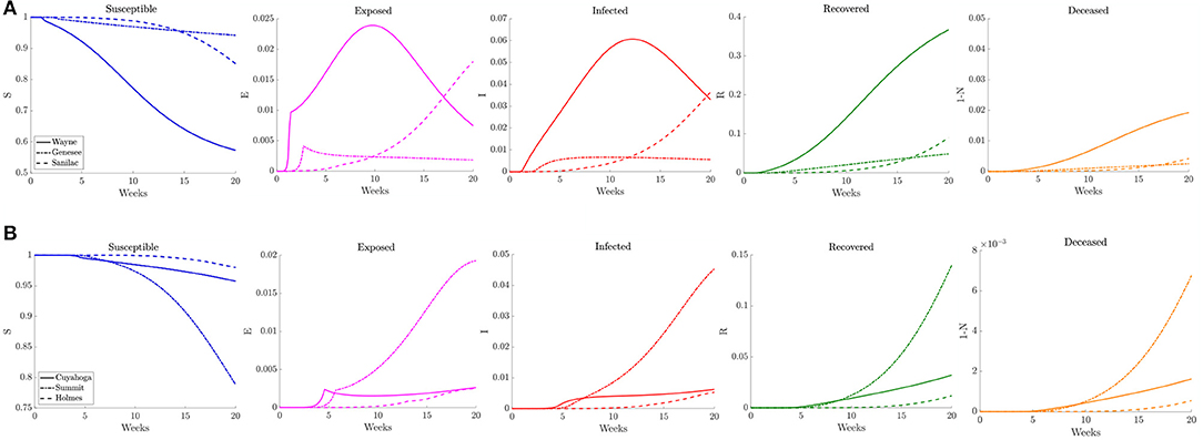
Figure 14. Plots of the relative (left to right) susceptible, exposed, infected, recovered, and deceased populations for the triggered physical distancing scenario (section 3.2.4) for (A) Wayne, Genesee, and Sanilac Counties in Southeast Michigan and (B) Cuyahoga, Summit, and Holmes Counties in Northeast Ohio. Note the relative scale for the y-axis.

4. Discussion

The outbreak of SARS-CoV2 in Wuhan, China, and its rapid spread within a few months across Europe and the United States has been closely followed in the hope to find ways to control and contain the pandemic. One important question is, where the pandemic will hit next, and how severely the next hotspot will be affected. The geographic pattern followed by the spread of COVID-19 has been rather consistent. As the epidemic moves into a region, the initial hotspots are typically urban centers with large population density and high contact rates, then the infection moves to less crowded communities, where the peak is reached at a later time. The rapidly changing situation and the need of swiftly updating the information based on the inflow of new data underline the importance of dynamic rather than static models, and the capability of model updating on a daily basis. The proposed Bayesian particle filtering approach combined with a metapopulation network model seeks to address these needs.

The Bayesian particle filtering algorithm is applied to a model on the community level that merges the asymptomatic pre-infected cohort and asymptomatic, infected, and infectious cohort. While this model simplification does not correctly account for the asymptomatic non-infectious period of COVID-19 that may be of some importance in modeling the spread, the significant gain is that the asymptomatic infectious cohort becomes tractable for state estimation, and allows us to directly infer on its size from the data consisting of only new infected symptomatic cases. In particular, in contrast to existing models, no assumptions about the relative sizes of the symptomatic and asymptomatic cohorts are needed. Despite this shortcoming of the model, a very promising feature is that our prediction of this ratio perfectly matches the best current estimate released by the CDC. We point out that adding the pre-infectious cohort in the model without loosing the observability of the asymptomatic cohort is not as straightforward as it may appear. Addressing this modeling challenge, and other technical challenges that the delay introduces, will be topics of future work.

Our contribution to the understanding of the geographical pattern of the COVID-19 transmission joins the spatial model of transmission in England and Wales [45], that uses census data from 2011 for population density and human mobility, and estimates the parameters from the China outbreak data. Our methodology and goals are close to those of the dynamic metapopulation network model in Li et al. [23] based on a network of cities in China. Because of the novelty of the SARS-CoV-2, the assumptions about important epidemiological parameters have been updated several times since the beginning of the outbreak, including the prevalence of asymptomatic transmission as well as incubation and recovery times, as reflected in the settings of these earlier models. Mutations in the pathogen as it moves from continent to continent may require calibration of the parameter values for the geographical region of interest. Importantly, our model does not rely on parameters estimated from data from Asia or Europe, but estimates them directly from the local data. The current study concentrated on 18 counties in Northeast Ohio and 19 counties in Southeast Michigan, representing a mix of urban, suburban and rural setting. However, as the network is constructed on the basis of publicly available mobility data from the US Census database, the model can be adapted to any county level network.

As the results show, the time courses of the reproduction number and the transmission rate parameter for the model describing the dynamics of the epidemics in each node, estimated from the daily counts of recorded infections, vary significantly from county to county, following a pattern that can be understood in terms of the network connectivity and social distancing measures. In particular, the time courses of the transmission rate in the individual counties clearly demonstrate the effect of mitigation measures on this parameter, mostly in the form of reduced mobility and social distancing. During the observation period included in this study, Ohio started the Stay at home Ohio program on March 15, 2020, and canceled the Democratic primary elections, originally scheduled for March 17. A similar Stay at home Michigan program became effective on March 23, 2020, although the Michigan primary elections had taken place, as scheduled, on March 10.

The individual county level models were used to inform the two network models, and it was found that the computed simulations reproduce satisfactorily the observed spreading patterns in both cases, showing the characteristic pattern of the epidemic moving from dense urban centers outward, following the highways that directly affect the commuter traffic between the communities. Figure 15 shows the block of counties in Michigan (a) and Ohio (e) in the network models and the main highways traversing them (Figures 15B,F). Panels Figures 15C,G show the daily reported number of infections on April 4, 2020 in the Michigan counties, and on April 16, 2020 in the Ohio counties, which are remarkably similar to the model predictions, shown in Figures 15D,H. The numerical simulations with altered rates of daily contacts clearly demonstrate the effectiveness of social distancing measures in slowing down the epidemics. In particular, two findings are worth highlighting: First, the simulations demonstrate that compared to non-diversified social distancing measures in all counties, equally effective is a strategy in which social distancing measures are enforced only if the relative frequency of infected individuals exceed a certain threshold. This finding suggests an efficient and economically less burdensome alternative to state-wide blanket mitigation measures, however, it relies heavily on availability of extensive testing. Our model echoes the finding in Karatayev et al. [46] that local re-opening, and re-closing according to the prevalence of infections can be a very effective mitigation measure even without limiting intercounty communication. The second finding, in light of the simulations, is the relative inefficiency of travel restrictions. While mobility is undoubtedly the key factor in spreading of epidemics, somewhat counterintuitively, the volume seems to be only a secondary factor, determining how fast the spreading takes place, and not how widely the epidemics spreads. This finding is in line with the discussion in earlier [13–16], and more recent [47] literature.

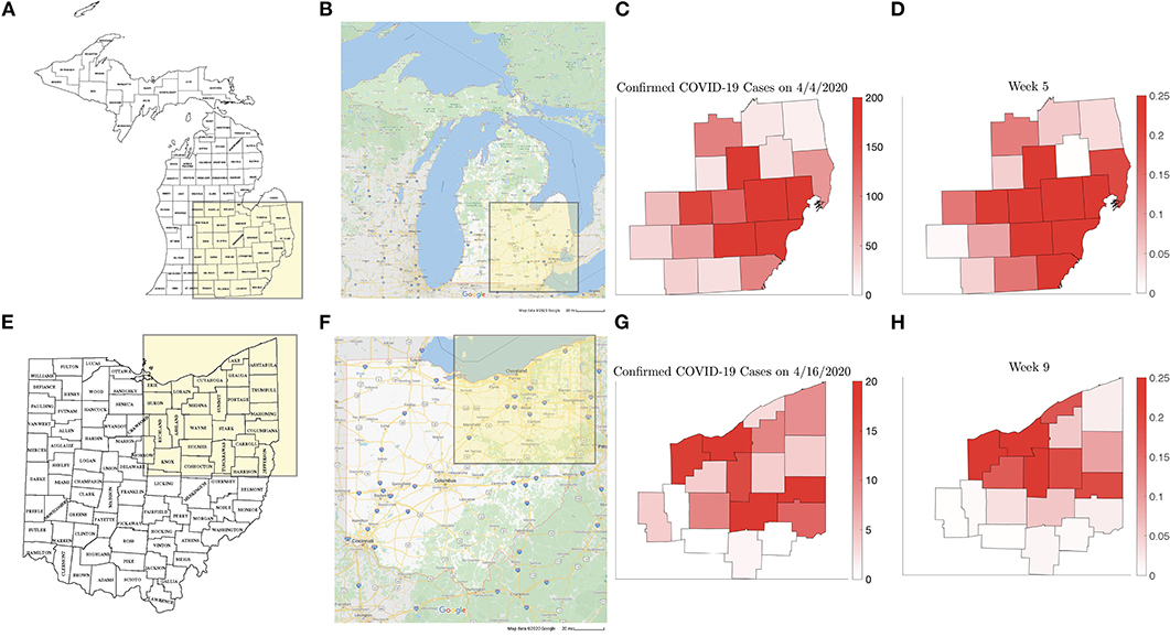
Figure 15. Counties in the Michigan (A) and Ohio (E) networks, (Map data © 2020 Google) with the main highways traversing them (B,F). (C,G) show the new number of infected on April 4, 2020 and on April 16, 2020, respectively, with the corresponding model predictions (D,H).

The current model does not include demographic information such as age structure of the population that is believed to be an important factor in predicting the severity and outcome of the epidemics for different communities. The demographic data can be introduced in the metapopulation model in a straightforward manner, and preliminary tests are underway. Simultaneous and parallel estimation of the parameters of connected communities will be part of the future work. As demonstrated in earlier articles by the authors [48], the particle filtering technique is particularly amenable for parallel computing.

Data Availability Statement

The original contributions presented in the study are included in the article/Supplementary Material, further inquiries can be directed to the corresponding author/s.

Author Contributions

All authors participated in the design of the models, methodology, and experiments, and assessment of their relevance. DC, AH, and ES contributed the computer coding and testing. All authors participated in the writing of the article.

Funding

The work of DC was partly supported by NSF grants DMS-1522334 and DMS-1951446, and the work of ES was partly supported by NSF grant DMS-1714617.

Conflict of Interest

The authors declare that the research was conducted in the absence of any commercial or financial relationships that could be construed as a potential conflict of interest.

Supplementary Material

The Supplementary Material for this article can be found online at: https://www.frontiersin.org/articles/10.3389/fphy.2020.00261/full#supplementary-material

References

1. Perc M, Gorišek Miksić N, Slavinec M, Stožer A. Forecasting Covid-19. Front Phys. (2020) 8:127. doi: 10.3389/fphy.2020.00127
2. Kermack WO, McKendrick A. A contribution to the mathematical theory of epidemic. Proc R Soc Lond. (1927) 115:700–21. doi: 10.1098/rspa.1927.0118
3. Anderson RM, May RM. Directly transmitted infections diseases: control by vaccination. Science. (1982) 215:1053–60. doi: 10.1126/science.7063839
4. Anderson RM, May RM. Vaccination and herd immunity to infectious diseases. Nature. (1985) 318:323–9. doi: 10.1038/318323a0
5. Keeling MJ, Rohani P. Modeling Infectious Diseases in Humans and Animals. Princeton, NJ: Princeton University Press (2011).
6. Levins R. Some demographic and genetic consequences of environmental heterogeneity for biological control. Am Entomol. (1969) 15:237–40. doi: 10.1093/besa/15.3.237
7. Perra N, Balcan D, Gonçalves B, Vespignani A. Towards a characterization of behavior-disease models. PLoS ONE. (2011) 6:e23084. doi: 10.1371/journal.pone.0023084
8. Wang L, Li X. Spatial epidemiology of networked metapopulation: an overview. Chinese Sci Bull. (2014) 59:3511–22. doi: 10.1007/s11434-014-0499-8
9. Balcan D, Hu H, Goncalves B, Bajardi P, Poletto C, Ramasco JJ, et al. Seasonal transmission potential and activity peaks of the new influenza A (H1N1): a Monte Carlo likelihood analysis based on human mobility. BMC Med. (2009) 7:45. doi: 10.1186/1741-7015-7-45
10. Balcan D, Vespignani A. Phase transitions in contagion processes mediated by recurrent mobility patterns. Nat Phys. (2011) 7:581–6. doi: 10.1038/nphys1944
11. Balcan D, Vespignani A. Invasion threshold in structured populations with recurrent mobility patterns. J Theor Biol. (2012) 293:87–100. doi: 10.1016/j.jtbi.2011.10.010
12. Ajelli M, Gonçalves B, Balcan D, Colizza V, Hu H, Ramasco JJ, et al. Comparing large-scale computational approaches to epidemic modeling: agent-based versus structured metapopulation models. BMC Infect Dis. (2010) 10:190. doi: 10.1186/1471-2334-10-190
13. Hollingsworth TD, Ferguson NM, Anderson RM. Will travel restrictions control the international spread of pandemic influenza? Nat Med. (2006) 12:497–9. doi: 10.1038/nm0506-497
14. Cooper BS, Pitman RJ, Edmunds WJ, Gay NJ. Delaying the international spread of pandemic influenza. PLoS Med. (2006) 3:e212. doi: 10.1371/journal.pmed.0030212
15. Tomba GS, Wallinga J. A simple explanation for the low impact of border control as a countermeasure to the spread of an infectious disease. Math Biosci. (2008) 214:70–2. doi: 10.1016/j.mbs.2008.02.009
16. Bajardi P, Poletto C, Ramasco JJ, Tizzoni M, Colizza V, Vespignani A. Human mobility networks, travel restrictions, and the global spread of 2009 H1N1 pandemic. PLoS ONE. (2011) 6:e16591. doi: 10.1371/journal.pone.0016591
17. Meloni S, Perra N, Arenas A, Gómez S, Moreno Y, Vespignani A. Modeling human mobility responses to the large-scale spreading of infectious diseases. Sci Rep. (2011) 1:62. doi: 10.1038/srep00062
18. Wang B, Cao L, Suzuki H, Aihara K. Safety-information-driven human mobility patterns with metapopulation epidemic dynamics. Sci Rep. (2012) 2:887. doi: 10.1038/srep00887
19. Wang L, Wang Z, Zhang Y, Li X. How human location-specific contact patterns impact spatial transmission between populations? Sci Rep. (2013) 3:1–10. doi: 10.1038/srep01468
20. Poletti P, Ajelli M, Merler S. The effect of risk perception on the 2009 H1N1 pandemic influenza dynamics. PLoS ONE. (2011) 6:e16460. doi: 10.1371/journal.pone.0016460
21. He X, Lau EHY, Wu P, Deng X, Wang J, Hao X, et al. Temporal dynamics in viral shedding and transmissibility of COVID-19. Nat Med. (2020) 30:10127–34. doi: 10.3389/fnins.2013.12345/abstract
22. Wölfel R, Corman VM, Guggemos W, Seilmaier M, Zange S, Müller MA, et al. Virological assessment of hospitalized patients with COVID-2019. Nature. (2020) 581:465–9. doi: 10.1038/s41586-020-2196-x
23. Li R, Pei S, Chen B, Song Y, Zhang T, Yang W, et al. Substantial undocumented infection facilitates the rapid dissemination of novel coronavirus (SARS-CoV2). Science. (2020) 368:489–93. doi: 10.1126/science.abb3221
24. American Community Survey;. Available online at: https://www.census.gov/programs-surveys/acs
25. Cheng HY, Jian SW, Liu DP, Ng TC, Huang WT, Lin HH. Contact tracing assessment of COVID-19 transmission dynamics in Taiwan and risk at different exposure periods before and after symptom onset. JAMA Intern Med. (2020) 1:e202020. doi: 10.1001/jamainternmed.2020.2020
26. Sood N, Simon P, Ebner P, Eichner D, Reynolds J, Bendavid E, et al. Seroprevalence of SARS-CoV-2–specific antibodies among adults in Los Angeles County, California, on April 10-11, 2020. JAMA. (2020) 323:2425–7. doi: 10.1001/jama.2020.8279
27. Bendavid E, Mulaney B, Sood N, Shah S, Ling E, Bromley-Dulfano R, et al. Covid-19 antibody seroprevalence in Santa Clara county, California. medRxiv. (2020).
28. Calvetti D, Hoover A, Rose J, Somersalo E. Bayesian dynamical estimation of the parameters of an SE (A) IR COVID-19 spread model. arXiv preprint arXiv:2005.04365. (2020).
29. Liu J, West M. Combined parameter and state estimation in simulation-based filtering. In: Doucet A, de Freitas JFG, Gordon NJ, editors. Sequential Monte Carlo Methods in Practice. New York, NY: Springer (2001). p. 197–223.
30. Arnold A, Calvetti D, Somersalo E. Parameter estimation for stiff deterministic dynamical systems via ensemble Kalman filter. Inverse Probl. (2014) 30:105008. doi: 10.1088/0266-5611/30/10/105008
31. Arnold A, Calvetti D, Somersalo E. Linear multistep methods, particle filtering and sequential Monte Carlo. Inverse Probl. (2013) 29:085007. doi: 10.1088/0266-5611/29/8/085007
32. Arnold A, Calvetti D, Gjedde A, Iversen P, Somersalo E. Astrocytic tracer dynamics estimated from [1-11C]-acetate PET measurements. Math Med Biol. (2015) 32:367–82. doi: 10.1093/imammb/dqu021
33. Centers for Disease Control and Prevention. COVID-19 Pandemic Planning Scenarios. (2020). Available online at: https://www.cdc.gov/coronavirus/2019-ncov/hcp/planning-scenarios.html (accessed May 26, 2020).
34. King AA, Domenech de Cellès M, Magpantay FM, Rohani P. Avoidable errors in the modelling of outbreaks of emerging pathogens, with special reference to Ebola. Proc R Soc B Biol Sci. (2015) 282:20150347. doi: 10.1098/rspb.2015.0347
35. Delamater PL, Street EJ, Lesley TF, Yang YT, Jacobsen KH. Complexity of the basic reproduction Number (R0). Emerg Infect Dis. (2019) 25:1–4. doi: 10.3201/eid2501.171901
36. Diekmann O, Heesterbeek APJ, Metz JAJ. On the definition and computation of the basic reproduction ratio R0 in models for infectious diseases in heterogeneous populations. J Math Biol. (2005) 28:365–82. doi: 10.1007/BF00178324
37. Diekmann O, Heesterbeek J, Roberts MG. The construction of next-generation matrices for compartmental epidemic models. J R Soc Interface. (2010) 7:873–85. doi: 10.1098/rsif.2009.0386
38. Dietz K. The estimation of the basic reproduction number for infectious diseases. Stat Methods Med Res. (1993) 2:23–41. doi: 10.1177/096228029300200103
39. Heesterbeek JAP. A brief history of R0 and a recipe for its calculation. Acta Biotheor. (2002) 50:189–204. doi: 10.1023/A:1016599411804
40. Heffernan JM, Smith RJ, Wahl LM. Pespectives on the basic reproductive ratio. J R Soc Interface. (1990) 2:365–82. doi: 10.1098/rsif.2005.0042
41. Li JBlakeley D, et al. The failure of R0. Comput Math Methods Med. (2011) 2011:527610. doi: 10.1155/2011/527610
42. Lauer SA, Grantz KH, Bi Q, Jones FK, Zheng Q, Meredith HR, et al. The incubation period of coronavirus disease 2019 (COVID-19) from publicly reported confirmed cases: estimation and application. Ann Intern Med. (2020) 172:577–82. doi: 10.7326/M20-0504
43. Singhal T. A review of coronavirus disease-2019 (COVID-19). Indian J Pediatr. (2020) 87:281–6. doi: 10.1007/s12098-020-03263-6
44. Tindale L, Coombe M, Stockdale JE, Garlock E, Lau WYV, Saraswat M, et al. Transmission interval estimates suggest pre-symptomatic spread of COVID-19. MedRxiv. (2020). doi: 10.1101/2020.03.03.20029983
45. Danon L, Brooks-Pollock E, Bailey M, Keeling MJ. A spatial model of COVID-19 transmission in England and Wales: early spread and peak timing. medRxiv. (2020). doi: 10.1101/2020.02.12.20022566
46. Karatayev V, Anand M, Bauch CT. The far side of the COVID-19 epidemic curve: local re-openings based on globally coordinated triggers may work best. medRxiv. (2020). doi: 10.1101/2020.05.10.20097485
47. Espinoza B, Castillo-Chavez C, Perrings C. Mobility restrictions for the control of epidemics: when do they work?. [Preprint]. arXiv:1908.05261v1, (2019).
Keywords: SEIR model, connectivity matrix, Bayesian parameter estimation, particle filter, uncertainty quantification, predictive envelopes
Citation: Calvetti D, Hoover AP, Rose J and Somersalo E (2020) Metapopulation Network Models for Understanding, Predicting, and Managing the Coronavirus Disease COVID-19. Front. Phys. 8:261. doi: 10.3389/fphy.2020.00261
Received: 11 May 2020; Accepted: 10 June 2020;
Published: 19 June 2020.
Edited by:
Matjaž Perc, University of Maribor, SloveniaReviewed by:
Lin Wang, University of Cambridge, United KingdomChris Bauch, University of Waterloo, Canada
Copyright © 2020 Calvetti, Hoover, Rose and Somersalo. This is an open-access article distributed under the terms of the Creative Commons Attribution License (CC BY). The use, distribution or reproduction in other forums is permitted, provided the original author(s) and the copyright owner(s) are credited and that the original publication in this journal is cited, in accordance with accepted academic practice. No use, distribution or reproduction is permitted which does not comply with these terms.
*Correspondence: Alexander P. Hoover, ahoover1@uakron.edu