Multi-Loop Radio Frequency Coil Elements for Magnetic Resonance Imaging: Theory, Simulation, and Experimental Investigation
 Roberta Frass-Kriegl1
  Sajad Hosseinnezhadian2
  Marie Poirier-Quinot2
  Elmar Laistler1
  Jean-Christophe Ginefri2*
- 1Division MR Physics, Center for Medical Physics and Biomedical Engineering, Medical University of Vienna, Vienna, Austria
- 2IR4M (Imagerie par Résonance Magnétique et Multi-Modalités), UMR 8081, Université Paris-Sud/CNRS, Université Paris-Saclay, Orsay, France
Magnetic resonance imaging (MRI) is a major imaging modality, giving access to anatomical and functional information with high diagnostic value. To achieve high-quality images, optimization of the radio-frequency coil that detects the MR signal is of utmost importance. A widely applied strategy is to use arrays of small coils in parallel on MR scanners equipped with multiple receive channels that achieve high local detection sensitivity over an extended lateral coverage while allowing for accelerated acquisition and SNR optimization by proper signal weighting of the channels. However, the development of high-density coil arrays gives rise to several challenges due to the increased complexity with respect to mutual decoupling as well as electronic circuitry required for coil interfacing. In this work, we investigate a novel single-element coil design composed of small loops in series, referred to as “multi-loop coil (MLC).” The MLC concept exploits the high sensitivity of small coils while reducing sample induced noise together with an extended field of view, similar to arrays. The expected sensitivity improvement using the MLC principle is first roughly estimated using analytical formulae. The proof of concept is then established through fullwave 3D electromagnetic simulations and validated by B1 mapping in MR experiments on phantom. Investigations were performed using two MLCs, each composed of 19 loops, targeting MRI at high (3 T) and at ultra-high field strength (7 T). The 3 T and 7 T MLCs have an overall diameter of 12 and 6 cm, respectively. For all investigated MLCs, we demonstrate a sensitivity improvement as compared to single loop coils. For small distances inside the sample, i.e., close to the coil, a sensitivity gain by a factor between 2 and 4 was obtained experimentally depending on the set-up. Further away inside the sample, the performance of MLCs is comparable to single loop coils. The MLC principle brings additional degrees of freedom for coil design and sensitivity optimization and appears advantageous for the development of single coils but also individual elements of arrays, especially for applications with a larger area and shallow target depth, such as skin imaging or high-resolution MRI of brain slices.
Introduction
Radio frequency (RF) coils are the front end of the instrumental chain of a magnetic resonance imaging (MRI) system. They are used to generate the RF magnetic field that excites the nuclear spins, and to detect the MR signal, i.e., the RF signal induced by the rotating nuclear magnetization during relaxation. Consequently, RF coils play a major role in MRI since they are the link between the scanner and the sample to be imaged. In order to perform MRI with high diagnostic value, i.e., with high spatial resolution and high signal to noise ratio (SNR), it is of utmost importance to optimize the sensitivity of the RF coil with respect to both, the targeted clinical application and the MRI set-up.
The sensitivity factor of the RF coil quantifies the contribution of the coil to the overall SNR and represents its efficiency to detect the MR signal while minimizing the noise involved in the MR experiment [1]. The two main noise sources are the noise of the coil itself and the noise induced in the coil by the sample [2]. In most clinical MRI applications (typical field strength ≥ 1.5 T), targeting large anatomical sites (e.g., brain, knee) and employing large RF coils (i.e., diameters of several cm), the sample noise largely dominates over the internal coil noise, and is therefore the limiting factor for achieving high detection sensitivity.
The earliest and most often pursued solution to improve the RF coil detection sensitivity is to reduce the coil size, i.e., to use small surface coils [3–5]. This increases the magnetic coupling between the coil and the sample, thus increasing the amplitude of the detected MR signal. In addition, the equivalent volume of sample seen by the coil is reduced and, therefore also the sample induced noise. However, the limited field of view (FoV) of small coils reduces the accessible region of interest (ROI) and may be problematic for applications targeting anatomical regions that extend over an area that is large compared to the target depth.
To overcome this, a widely applied strategy is to use arrays of small coils together with MR scanners featuring multiple receive channels [6–8]. Arrays benefit from the high local detection sensitivity of small surface coils while achieving a lateral coverage comparable to large coils, and are now used in numerous clinical applications of MRI [9]. However, the development of high-density coil arrays evokes additional technological challenges [9, 10] due to the increased complexity with respect to mutual coupling between coils and electronic circuitry required for coil interfacing. Especially the realization of arrays with very small elements becomes impractical either due to fabrication issues with the coil elements themselves, or due to space requirements for the interface components and preamplifiers. On top of that, high-density arrays entail a significant increase of cost due to the high amount of required electronic components and the need for a high number of acquisition channels at the MR scanner.
In this work, we investigate a novel coil design that aims at achieving some benefits of coil arrays as compared to large single loop coils (SLCs), i.e., reduce the sample induced noise by using small coils and achieve a large FoV. Although this novel design doesn't represent an actual alternative to coil arrays, since it neither allows for parallel imaging nor SNR optimization by combining the signals of individual channels with optimal weights, it aims at a comparable sensitivity gain in comparison to large SLCs while relaxing constraints in terms of complexity and cost.
The general concept of this work is to investigate single coil elements composed of small loops in series, in contrast to the coil array principle where the coils are independent and operated in parallel. The association of small loops in series results in a single coil element composed of multiple loops, subsequently referred to as “multi-loop coil (MLC).” MLCs appear particularly advantageous for reducing sample-induced noise that varies with the loop radius to the power of three, while the equivalent noise voltages induced in each of the loops are summed linearly since they are in series. The use of small loops in series may also improve the magnetic coupling between the coil and the sample because the magnitude of the detected MR signal is inversely proportional to the loop radius. Consequently, a significant improvement in detection sensitivity is expected by using MLCs.
Few works reported the use of small loops associated to larger coils, either employing various sized small loops in series to reinforce and homogenize the magnetic coupling of the coil to the sample [11] or employing small loops of the same size equally distributed around a large loop [12, 13], with connections between small loops being alternately reversed so that the magnetic field is in phase. While these two investigations are supported by the same conceptual consideration as the present work, their targets are different, and they face several limitations regarding the freedom for loops positioning and number. Also, in both cases, a large loop is used, which counterbalances the benefit of using small loops and sets a limit to the achievable sensitivity improvement. In addition, an investigation on the effective improvement of the overall detection sensitivity has not been performed so far, neither by simulation nor by MRI experiments.
In this paper, we introduce the theoretical background supporting the MLC principle involving equations for sample and coil losses as well as for the magnetic field produced per unit of current. We present an electromagnetic simulation study to evaluate the MR performance of MLCs and, in particular, the improvement in terms of transmit efficiency, i.e., the magnetic field produced per square root of input power. We show experimental results obtained by MRI, i.e., maps of the transmit efficiency that aim at validating the simulation results and at experimentally demonstrating the sensitivity improvement achieved by MLCs as compared to SLCs.
Theory
RF Coil Sensitivity
An RF coil can be modeled as a resonant RLC circuit (resistance R, inductance L, capacitance C) tuned to the Larmor frequency of interest and matched to the input impedance of the MR scanner, i.e., typically 50 Ohm. The sensitivity factor of the RF coil SRF, which represents the contribution of the coil to the overall SNR, is the ratio of the induction coefficient, defined as the magnetic field, B1, per unit current, I, produced by the coil and the equivalent noise voltage associated to the losses involved in an MRI experiment.
where ReqTeq is the sum of the temperature-weighted resistances associated to different dissipative media and loss mechanisms.
The complete electromagnetic approach to derive expressions for B1 and losses is given in the literature (see for example [14] p. 127 for losses and p. 206 for B1/I). Starting from the AC source-current in the coil, one can derive a vector potential. From this the currents induced in the media can be determined, which in general have two components, the eddy current depending on conductivity, and the displacement current depending on permittivity. Using Maxwell-Ampère's equation, one can calculate the magnetic field inside the media originating foremost from the source-current but also from the currents induced in the media. The integral over the real part of the induced currents divided by the conductivity of the media provides the corresponding power loss density. Finally, using Ohm's law, the equivalent resistance is obtained from the power loss density and the current in the coil.
This approach leads to complex integral equations that cannot be solved analytically and require the use of advanced electromagnetic solvers. However, simplified formulae for B1 and losses neglecting propagation effects have been proposed (see below). Thus, B1 can be calculated using Biot-Savart's law, neglecting losses due to displacement currents. This approximation is valid if the dimensions of the ROI are small compared to the operating wavelength. For surface coils, when the depth of the targeted ROI does not exceed 10 cm, this assumption is typically fulfilled for field strengths up to 3 T.
Induction Coefficient
The induction coefficient of the coil, , is the magnetic coupling efficiency of the coil to the sample and is representative of the detected amount of MR signal. , depends on the area through which the nuclear magnetic flux passes and is set by the winding shape of the coil only.
For a single-turn circular coil of radius a, the theoretical expression for in Cartesian coordinates is given in [15]:
with the vacuum permeability μ0, standard elliptical integrals E(k2) and K(k2), and the following correspondences:
Along the coil axis, z, the above equations simplify, and the induction coefficient of the coil is expressed as:
For distances that are small compared to the coil radius, it varies roughly as a−1, explaining why small surface coils perform better than large ones when investigating ROIs located at the surface of the body. Further away from the coil, i.e., for distances large compared to the coil radius, the induction coefficient varies as a2 which disfavors smaller coils. However, this can be counterbalanced by combining several small coils operating constructively, since the total induction coefficient is the vector sum of the individual induction coefficients and can tend to equalize that of a large coil at long distance.
Dominant and Non-dominant Noise Sources in MRI
The equivalent noise voltage illustrates the total energy dissipated during the MR experiment. It is proportional to the square-root of the sum of equivalent temperature-weighted resistances according to respective dissipation rates and local temperatures in the different media, ReqTeq. Several noise mechanisms may be involved in MR experiments and a quantitative comparison of their respective contribution to the overall noise has to be done to identify suitable strategies to improve the RF sensitivity of the coil. The two main noise mechanisms to be considered in current biomedical applications of MRI are the noise of the coil itself and the noise induced in the coil by the sample, i.e., magnetically coupled sample noise [2].
In addition, several, usually non-dominant, noise mechanisms can potentially be involved in MR experiments. For instance, capacitively-coupled sample noise, which tends to be more significant at high field strength [16], can be reduced to a negligible level by using distributed tuning capacitors and inductive coupling transformers [17]. Other noise mechanisms, such as the spin noise [18] and the radiation noise [19], are of marginal relevance for current clinical MRI applications, i.e., below 300 MHz (i.e., 1H Larmor frequency at 7 T). Lastly, the use of electronic components and active devices may introduce additional losses, but they are usually minimized by optimizing the circuit design, e.g., placing high-gain low-noise preamplifiers as close as possible to the coil port.
Magnetically Coupled Sample Noise
Magnetically coupled sample noise is strongly related to the coupling efficiency of the coil, as the corresponding noise voltage is induced in the coil via the same physical pathway as the MR signal. Neglecting displacement currents as explained above, and considering again a circular loop of radius a placed at a distance s to a semi-infinite conducting sample with conductivity σ, the following approximate formula [20] of the sample induced resistance RS can be used in many practical situations:
Besides the quadratic dependence of RS on the operating frequency, indicating that these losses may be predominant over other losses at high field strength, it can be observed that RS varies as the power of 3 with the coil radius. This explains the large advantage of using small coils when sample noise dominates. It can be noticed that for coils with a radius that is small compared to the distance between the coil and the sample, the arctan-function varies as a, and the sample induced resistance then depends on the coil radius as the power 4. This consideration is the basis for the pinpoint coil concept that showed the potential improvement in sensitivity by using very small coil when the sample noise dominates, even for imaging regions located deep inside the sample [21].
When using several coils, in parallel as in arrays, or in series as in MLCs, the overall sample induced noise is larger than the sum of the sample induced noise in all individual loops. This noise increase is due to electrical coupling between the coils via the sample, referred to as noise correlation [6]. The analytical formulae to calculate the mutual resistance of several coils implies the determination of spatial distribution of the electric fields produced by all coils, and requires advanced computations [22] that are beyond the scope of the presented analytical evaluation of MLCs. Alternatively, one can consider a relative increase of the sample induced noise based on the electrical coupling coefficient as a function of the distance between loops [6]. The electric coupling coefficient between two coils can be defined in analogy to magnetic coupling:
Where RSik is the mutual resistance between the coil i and coil k and RSi, RSk are the sample induced resistance in the coils when isolated, i.e., without noise correlation, given by Equation (12). In the MLC design, all loops have the same sample induced resistance when large enough phantoms are employed, i.e., RSi = RSk. The value of the total sample resistance is then the sample induced resistance of each loop isolated plus twice the mutual resistance between loops:
Coil Noise
The standard technology to fabricate RF coils employs wound conducting wires intersected by lumped element capacitors. In this case, the total coil losses account for the ohmic losses of the winding as well as the real losses of the capacitors used to tune the coil.
The general formula for the ohmic resistance of a conducting loop of radius a made of a wire of radius r, with electrical resistivity ρ, and skin-depth , can be approximated by the following expression [23] when operating at frequencies high enough so that δ < < r:
In the case of a conducting loop of outer radius a made of a flat conducting strip of width w the above expression becomes [23]:
This estimation only considers the “classical” skin effect and neglects the lateral skin effect contributions for flat strip conductors, which tend to dominate especially at higher frequencies [24–26]. In addition, the conductor losses of multi-turn and multi-loop coils can be increased due to the proximity effect [27], which constrains the current distribution to an even smaller region than the skin effect. This loss contribution depends on the exact coil design and is neglected for the following rough loss estimation.
Capacitor losses originate from two different phenomena with relative contributions depending on the operating frequency. The first component are dielectric losses inside the capacitor material itself characterized by the loss tangent, tanδ ([14] p. 127). Second, the metallic parts of the capacitors, such as contacts for soldering, generate metallic losses, similarly to conductors. The total losses of capacitors, referred to as the equivalent series resistance (ESR) are the sum of the dielectric and metallic resistances, and are usually available from data sheets. Regarding the typical operating frequency range of RF coils in MRI, and accounting for the conductivity and permittivity of typical capacitor materials, metallic losses dominate over dielectric losses. In addition to the capacitor losses, losses associated to solder joints used to mount the capacitors onto the coil winding should be considered as it may have a significant contribution to the overall noise [23].
One can notice that when employing other technologies than that of lumped components to fabricate the coil, the two above mentioned noise sources are still of concern. Considering the case of self-resonant coils based on the transmission line principle (e.g., [28]), losses within the substrate, similarly to capacitors losses, may contribute to the overall coil noise and should be considered. This is particularly of concern when using low quality substrates, such as FR4 or Polyimide (e.g., Kapton®) whose loss tangent limits the achievable overall quality factor of the coil. However, by choosing materials with a low loss tangent, such as Polytetrafluoroethylene (PTFE), dielectric losses within the substrate can be kept at a negligible level compared to the ohmic losses of the coil conductor.
Rough Estimate of the Sensitivity Improvement Expected With MLCs
As discussed above, reducing the coil size can provide a significant reduction of the sample induced losses together with an increase of the induction coefficient. In this section, we roughly evaluate the theoretical gain in sensitivity expected by using an MLC as compared to an SLC achieving an equivalent FoV. In this regard, we will consider an SLC of radius A and compare its losses and induction coefficient to those of an MLC composed of N small loops of radius a = connected in series.
Estimation of the Induction Coefficient
Considering sample-to-coil distances small compared to the coil radius, which corresponds to the usual case when using surface coils, the induction coefficient is inversely proportional to the coil radius (see Equation 11). Consequently, a small loop of radius , will produce a B1/I at close distance along its axis that is -times higher than that of a larger loop of radius A. It can be assumed that in the case of N small loops in series, close to one small loop the other loops will not produce a significant B1 along its axis. So, at close distance from the loops, only a benefit from the size reduction can be expected using the MLC principle. Further away from the loop, B1/I on its axis varies as the square of the radius. In this case, N small loops of radius a, are expected to produce a B1/I that is comparable to that of a larger loop of radius A. It finally appears from this rough estimate that MLCs achieve an induction coefficient higher or equal to that of a large coil.
Estimation of Sample Losses
When considering the sample resistance dependency on the coil radius, as shown in Equation (12), and for sample to coil distances small as compared to the coil radius, it appears that a large loop of radius A will result in a sample-induced resistance proportional to A3, whereas N small loops of radius , will result at a first glance in a total sample-induced resistance proportional to . Consequently, a significant decrease of the sample losses is expected by using MLCs as compared to SLCs covering a comparable surface area. However, this estimate does not account for the increase of the total sample losses due to mutual resistances between the loops. Indeed, the use of N loops in series will add N × (N − 1) mutual resistances, having different amplitude depending on the distance between the considered coupled loops. As the amplitudes of the mutual resistances cannot be estimated for arbitrary MLC geometries, the noise correlation effect was not accounted for in the rough estimation of the gain in sensitivity expected by using MLCs as compared to SLCs since it aims only at illustrating the concept supporting the present investigation.
Estimation of Coil Losses
According to Equations (15) and (16), the ohmic resistance associated to the coil winding of N loops of radius in series is -times higher than that of an SLC of radius A assuming identical wire radius.
The equivalent series resistance of the capacitors depends on the number of capacitors which is proportional to the total conductor length so as to maintain the same ratio between operating wavelength and uninterrupted conductor length. Since the total length of N small loops of radius in series is -times longer than that of a loop of radius A, the number of required capacitors for the N small loops is -times higher than for the single large loop. So, at a first glance, it could be concluded that the resistance of the capacitors for the N small loops will be -times higher than for the large loop. When using more distributed capacitors the capacitance value has to be increased so as to reach the same resonance frequency. As a general tendency, the higher the capacitance value is, the lower the equivalent series resistance of the capacitors is; therefore, in practice the total resistance of the capacitors in case of N small loops may be increased by a factor lower than . However, in some cases (depending on the type of capacitors and the operating frequency), the above mentioned tendency does not hold true, i.e., capacitors with lower capacitance value exhibit a lower, or comparable equivalent series resistance to capacitors with higher capacitance value. In conclusion, the total coil resistance, including ohmic and capacitors losses, of N loops of radius in series is increased by a factor of as compared to that of a loop with radius A.
Estimation of the Sensitivity Factor
Taking into account the above considerations on the influence of the number of loops on the resistances and the induction coefficient of the coils, one can estimate the global impact of using MLCs on the sensitivity factor. To do so, two cases are distinguished.
At short distances inside the sample, the induction coefficient of the MLC is -times higher than the one of an SLC of radius A.
In this case, the sensitivity factor achieved by MLCs, expressed as a function of the single loop parameters , is:
At long distances inside the sample, the induction coefficient of the MLC is comparable to the one of the SLC of radius A, and the sensitivity factor achieved by the MLC is:
As expected, the benefit of using an MLC as compared to a large SLC depends on the respective contribution of coil losses and sample induced losses and will be more pronounced when the sample losses are dominant. A rough analysis of the loss dependency on coil radius and operating frequency indicates that sample noise is dominant for large coils or at high frequency. In this case, MLCs can achieve a significant sensitivity improvement. In the other case, when coil losses contribute significantly to the total losses, the benefit of using MLCs is less but a non-negligible improvement may be still expected.
If the sample losses largely dominate over coil losses, the sensitivity factor of the MLC is increased in comparison to the SLC by a factor of N3/4 and a factor of N1/4 at short and long distances inside the sample, respectively.
As an intermediate case, considering that the coil losses are equal to the sample induced losses for a loop of radius A, i.e., RSA = RCA then at short distances:
And at long distances:
In the extreme case, when coil losses dominate over sample losses, corresponding to the less favorable case for using MLCs, the sensitivity factor achieved by the MLC as compared to the SLC is increased by a factor of N1/4 and decreased by a factor of N1/4 at short and long distances inside the sample, respectively.
As a general conclusion of the rough estimate of the expected improvement in sensitivity achieved by the use of MLCs, it appears that an MLC performs better than a large SLC in any case except when the coil noise of the large loop dominates over the sample induced noise for ROIs deep inside the sample.
Materials and Methods
Investigated Coils
We illustrate the sensitivity improvement achieved by the MLC principle by investigating two MLCs made of N = 19 loops in series. The general scheme and dimensions of the two investigated MLCs are shown in Figure 1A. The performance of each MLC is compared to that of an SLC shaving the same outer diameter. The scheme of the SLCs used for comparison is depicted in Figure 1B. So as to reduce capacitively coupled sample noise, the winding of the MLCs and the SLCs were segmented by 12 and 8 or 4 (for 3 T or 7 T SLCs) distributed tuning capacitors, respectively. In all cases, it is ensured that the segment length between two capacitors is small as compared to the operating wavelength. Within these constraints, the exact number of capacitors was chosen also according to practical reasons, e.g., reusing existing coil layouts. The two straight lines connected at the bottom of the coils' winding are for connecting the coaxial cable that relates the coil to the scanner interface, where each has a gap for placing balanced matching capacitors. The coil diameters were chosen so that the sample induced losses in the SLC can be assumed large as compared to the internal losses of the coil itself at the operating frequency [1], thus allowing to better evidence the sensitivity improvement achieved by the use of MLCs.
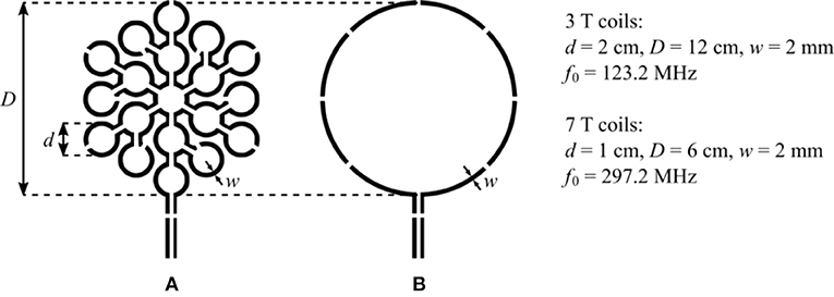
Figure 1. (A) General scheme of the investigated MLCs. Each MLC is composed of 19 loops of diameter d connected in series covering an equivalent circular surface of diameter D. (B) Scheme of the SLCs having a diameter D used for comparison. For all coils, the gaps in the coil winding are made for placing the distributed tuning capacitor, and the gaps on the two straight lines at the bottom of the coils' winding are made for placing the balanced matching capacitors.
All coils were fabricated using single layer copper of 35 μm thickness deposited on a 0.8 mm thick FR4 substrate. The conductor width was 2 mm for all coils. The coil patterns were produced using standard photolithographic processing.
Evaluation by Simulation
Analytical Estimation of the RF Sensitivity Factor Using the Quasi-Static Approximation
In order to evaluate more precisely the expected RF sensitivity factor of MLCs and validate the initial rough estimate of the sensitivity improvement on which the MLC concept is based, SRF maps were computed for the investigated MLCs and SLCs according to Equation (1) using Python. The induction coefficient was calculated using Equations (2)–(4). For the coil noise, conductor losses including the skin effect were estimated according to Equation (16); it is assumed that a more advanced model for conductor losses including lateral skin effect and proximity effect would only marginally influence the results as the total coil noise is dominated by capacitor and solder joint losses, and the overall noise is clearly sample dominated. Capacitor losses were modeled using the equivalent series resistances extracted from data sheets (CHB series, Exxelia, Paris, France), and solder joint resistances were estimated according to literature data [23], which were extrapolated with a -dependence for 297.2 MHz. The sample noise of the individual loops was calculated using Equation (12). In order to account for noise correlation between loops in MLCs, RSik values were estimated using approximated electrical coupling coefficients based on values determined by Roemer for square-shaped loops [6]. Interactions between all coils were accounted for, resulting in a total sample induced resistance being 60 times the sample induced resistance of one isolated small loop. When neglecting the noise correlation effect, as for the rough estimate of the RF sensitivity improvement discussed above, the total sample induced resistance is 19 times the one of an isolated small loop; i.e., noise correlation increases sample losses approximately by a factor of 3 for the investigated MLC design.
Fullwave 3D Electromagnetic Simulation
Due to the complex interactions between electromagnetic fields and the human body, especially at ultra-high frequency i.e., at ultra-high field strength, the quasi-static approximation is no longer valid and Biot-Savart law fails to accurately evaluate the B1 field of the coil. For this reason, fullwave 3D electromagnetic simulation (EMS) of RF coils has become mandatory to characterize their performances before fabrication. 3D EMS solve Maxwell's equations to obtain the electric and magnetic field distributions inside the sample that can further be used to calculate (transmit) and (receive) fields and the specific absorption rate (SAR).
In this study, we performed fullwave 3D EMS based on the finite difference time domain (FDTD) method [29] using a commercial software package (XFdtd 7.8 Remcom, State College, PA, USA). All investigated coils were modeled as perfectly conducting sheet bodies in 3D EMS. A box-shaped phantom positioned 1 mm below the coil was used as load (3 T: 170 × 170 × 150 mm; 7 T: 90 × 90 × 70 mm), with dielectric properties comparable to the phantom liquid used for the experimental evaluation described below (electrical conductivity σ = 0.71 S/m, relative permittivity ε = 63.86). Grid resolution varied from 0.5 mm for the coil conductors to 9 mm for regions outside the sample. All coil capacitors as well as the matching networks were replaced by 50 Ω voltage sources to enable circuit co-simulation [30, 31] (ADS, Keysight Technologies, USA), which shortens the total simulation time. In co-simulation, 50 Ω ports were replaced by respective lumped elements for tuning and impedance matching. Realistic loss estimations for the coil conductors, inductances, capacitances, and solder joints were modeled as resistances in series with the coil winding, in accordance with coil noise calculation for the analytical estimation. The air core inductor required for matching the 3 T SLC (see below) was assigned a Q of 200. Post-processing of the simulation data was performed in Matlab (Mathworks, Natick, MA, USA) using a dedicated in-house toolbox (SimOpTx, Center for Medical Physics and Biomedical Engineering, Medical University of Vienna, Austria) employing the quadratic form power correlation matrix formalism [32, 33]. MLCs and SLCs were compared in terms of transmit efficiency, i.e., per input power, as well as 10 g-averaged SAR.
Experimental Evaluation
Phantom
A canister (~18 × 13 × 28 cm) filled with saline solution (deionized H2O doped with 0.8 mL/L Gadolinium solution with a concentration of 279.32 mg/mL of Gadoteric acid, and 4 g/L NaCl resulting in a DC conductivity of σ = 0.65 S/m) was used as phantom load for bench measurements as well as for MR experiments at 3 T and 7 T. A photograph of the phantom with the 7 T MLC attached to it is shown in Figure 2.
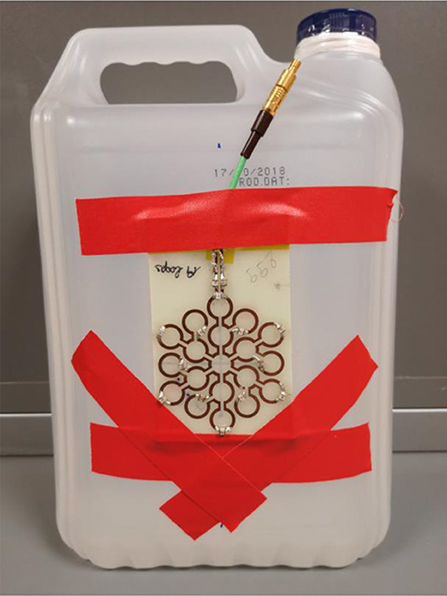
Figure 2. Photograph of the phantom with the 7 T MLC attached to it.
Bench Measurements
Tuning and matching of the coils were performed using small multi-layer non-magnetic high-Q ceramic capacitors (CHB series, Exxelia, Paris, France). Besides their MR compatibility, these capacitors were chosen to minimize the total associated ESR. For each coil, series tuning capacitors CS, a parallel tuning and matching capacitor CTM and two identical series matching capacitors CM with the values listed in Table 1 were used. In order to match the 3 T SLC to 50 Ω, an additional parallel inductor LM had to be incorporated in the matching network of this coil. As the coils were designed to operate in the sample noise dominated regime, this low-Q (~200) inductor is assumed to have negligible influence on the coil's MR performance.
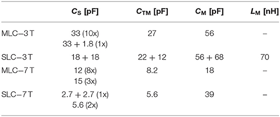
Table 1. Tuning and matching components.
All coils were connected to RG316 SPC coaxial cables (AXON' CABLE S.A.S. Montmirail, France), which served as connection to the two-port vector network analyzer (E5071C, Agilent, Santa Clara, USA) in bench measurements and as connection to the scanner interface in MR experiments.
Besides tuning and matching, also Q-factors of all investigated coils were measured in loaded and unloaded condition. This enabled us to ensure that sample noise is the dominant noise source as aimed for in this study, and to evaluate the sample noise reduction achieved by MLCs. Q-factors were measured using the single-loop probe method [34], while the coils were not connected to their respective matching networks. The influence of the single-loop probe was considered negligible when the reflection coefficient at its terminal was below −40 dB.
MRI Experiments
Both, 3 T and 7 T MR experiments were carried out on whole-body MRI systems (3T Prisma Fit and Magnetom 7T MRI, Siemens Healthcare, Erlangen, Germany), with the MLCs and SLCs operated in transmit-receive mode. For this purpose, a home built (for 3 T) and a third party (for 7 T; Stark Contrast, Erlangen, Germany) transmit-receive (T/R) switch with integrated low-noise preamplifiers (3 T: 0.5 dB noise figure, 27.0 ± 0.1 dB gain, Hi-Q.A. Inc., Carleton Place, Ontario, Canada; 7 T: 0.5 dB noise figure, 27.2 ± 0.2 dB gain, Siemens Healthcare, Erlangen, Germany) were used. At both field strengths, the same T/R switch and preamplifier were used for MLC and SLC, respectively, to avoid an influence of the interface components on the comparison.
With all investigated coils, flip angle maps were acquired in 13 coronal slices parallel to the coil plane using the saturated Turbo FLASH (satTFL) method [35]. The first slice was positioned directly at the phantom surface as close as possible to the coils; slice thickness was 3 mm and a spacing of 2 mm between consecutive slices was chosen. As the field of surface coils decreases rapidly along the coil axis, different amplitudes of the saturation pulse were chosen for the different slices in order to generate flip angles in the usable range [36]. The following sequence parameters were used at 3 T: repetition time TR = 12.64 s, echo time TE = 2.64 ms, 192 × 192 acquisition matrix, 1.5 mm × 1.5 mm in-plane pixel size, 1 average. At 7 T, the following parameters were applied: TR = 6.93 s, TE = 2.66 ms, 128 × 128 acquisition matrix, 1.5 × 1.5 mm in-plane pixel size, 4 averages. From measured flip angle distributions, maps normalized to the input power were calculated using an in-house written Matlab script (Mathworks, Natick, MA, USA) taking into account an insertion loss of −2 dB of the coil cables and the T/R-switches, determined on the bench.
High-resolution 3D gradient echo (GRE) sequences were employed to evaluate the imaging performance of the investigated coils. Data from these scans were used to calculate SNR maps in the central sagittal slice (i.e., in the yz-plane with B0 along the z-direction and the coil parallel to the xy-plane) with the basic ROI method for comparison of MLCs and SLCs. For 3 T measurements, the following sequence parameters were used: TR = 6.8 ms, TE = 2.88 ms, 288 × 234 × 224 acquisition matrix, 1 mm isotropic pixel size, flip angle α = 5°, pixel bandwidth BW = 545 Hz/Px, Tacq = 5:56 min. The sequence used in 7 T experiments had the following parameters: TR = 15 ms, TE = 6.86 ms, 256 × 256 × 128 acquisition matrix, 1 mm isotropic pixel size, α = 8°, BW = 100 Hz/Px, Tacq = 4:36 min.
Results
Q-Factors
Q-factors of the investigated MLCs and SLCs in unloaded and loaded condition are summarized in Table 2 for 3 T and 7 T, respectively. For comparison, also the Q-factors obtained from analytical calculations and fullwave simulations are listed. Further, the ratio of unloaded to loaded Q-values is calculated.
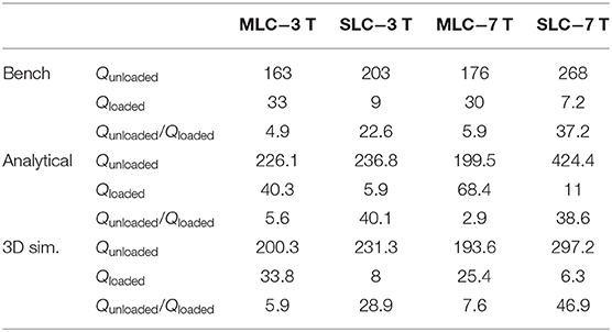
Table 2. Q-factors.
The measured Q-factors reflect well the behavior expected from theoretical considerations described in sections Estimation of sample losses and Estimation of coil losses. The unloaded Q-factor, inversely proportional to the coil noise, is lower for MLC than for SLCs. However, the Q-ratios show that the overall noise of the experiment, i.e., coil noise plus sample noise, is clearly dominated by the sample noise for all investigated configurations, as aimed for in the coil design process. The loaded Q-factors are higher for MLCs than for SLCs by factors of 3.67 and 4.17 at 3 T and at 7 T, respectively, demonstrating the sample noise reduction by employing the MLC principle. These ratios approach the theoretically expected reduction factor for the sample noise, i.e., , which was estimated under the approximations described above, and which could only be measured for pure sample noise dominance.
Sensitivity Factor and Transmit Efficiency
Maps of the calculated sensitivity factor, as well as the simulated and measured transmit efficiency, i.e., normalized to the input power (/), at different depths inside the sample, are summarized in Figures 3, 4 for 3 T and 7 T coils, respectively. The slice locations shown for calculations and simulations were chosen to correspond to the experimental data; for slices located further away from the coil, experimental maps appear too noisy for a visual comparison due to insufficient SNR of the flip angle mapping sequence. The analytical calculation does not aim at providing absolute SRF values but at estimating the expected sensitivity improvement. Therefore, all the sensitivity factors calculated analytically were normalized to the maximum value obtained with the MLCs at the shortest distance inside the sample.
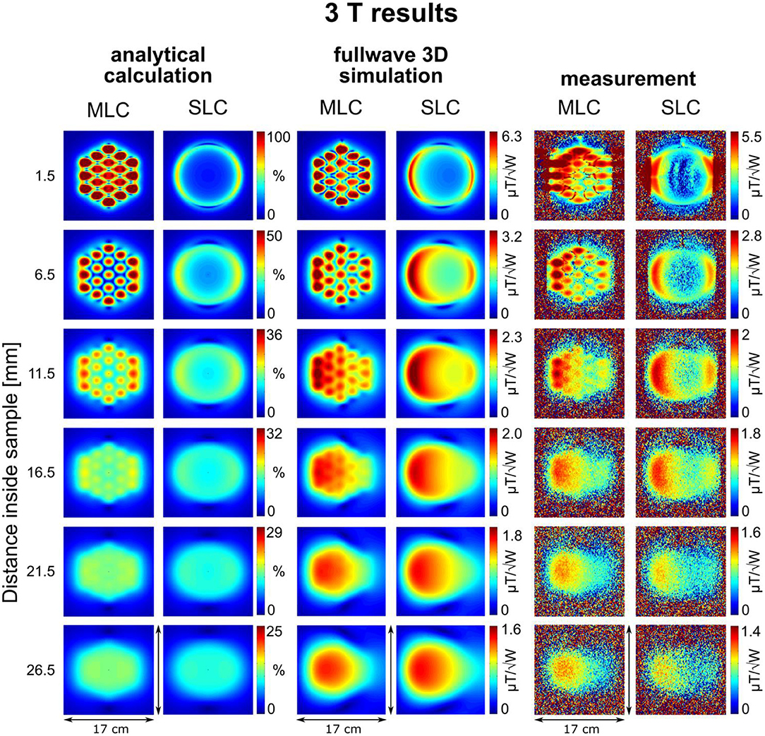
Figure 3. Maps of the calculated sensitivity factor, as well as the simulated and measured transmit efficiency at different depths inside the sample for 3 T coils. Calculated sensitivity factor values are normalized by the maximum sensitivity value obtained with the MLC at 1.5 mm distance inside the sample.
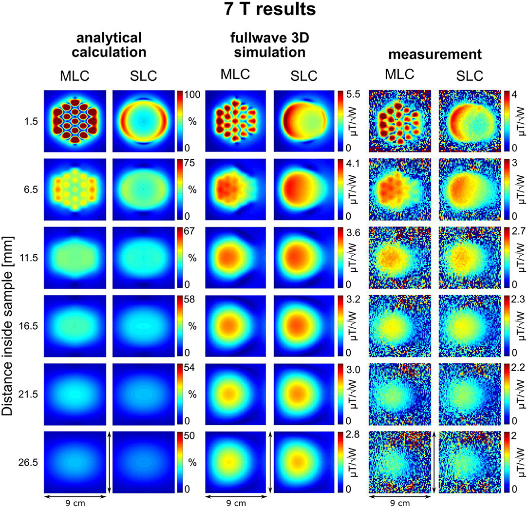
Figure 4. Maps of the calculated sensitivity factor, as well as the simulated and measured transmit efficiency at different depths inside the sample for 7 T coils. Calculated sensitivity factor values are normalized by the maximum sensitivity value obtained with the MLC at 1.5 mm distance inside the sample. Note that the dimensions of the maps are different from 3 T images due to the smaller coil size.
To enable a direct, quantitative comparison of MLCs and SLCs, ratios of MLCs' and SLCs' sensitivity factors and transmit efficiencies were calculated along the central axis of the investigated coils. These results are shown in Figure 5 for analytical calculations, fullwave 3D simulation and experimental data, for 3 T and 7 T coils, respectively. For experimental data, values in each slice were averaged over 10 × 10 and 5 × 5 pixel ROIs centered on the coil axis, for 3 T and 7 T, respectively, to limit the influence of measurement noise.
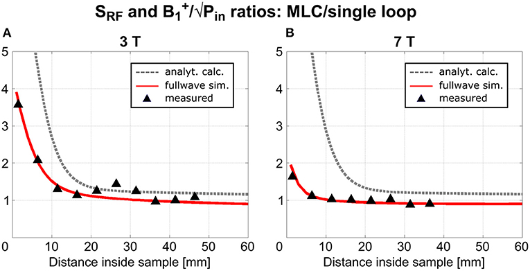
Figure 5. Ratios of RF sensitivity and transmit efficiency between MLCs and SLCs along the central coil axis—(A) for 3 T coils and (B) for 7 T coils.
An excellent qualitative agreement between fullwave simulations and measurements can be observed for maps as well as central axis profiles, at both, 3 T and 7 T. A maximum increase in transmit efficiency by a factor between 2 and 4 depending on field strength and coil size is obtained with MLCs in comparison to SLCs. A significant gain can be observed for distances up to the radius d/2 of the individual loops of the MLCs, i.e., 1 cm for 3 T and 0.5 cm for 7 T. For large distances (> d), the performance of MLCs and SLCs is comparable. For fullwave simulated data, the SLC marginally outperforms the MLC for distances larger than 3.4 cm at 3 T, and 1.2 cm at 7 T, respectively.
For MLCs, regions of high transmit efficiency directly below the small loops and low transmit efficiency in between loops can be observed in / maps. The impact of this behavior on the coils' performance in comparison to SLCs was analyzed more closely for 3D fullwave simulation data. The transmit efficiency ratio of MLC and SLC was computed for the whole phantom volume. The central sagittal and transversal slices as well as a coronal slice close to the coil plane are shown in Figures 6A, 7A for 3 T and 7 T, respectively. For the ROI shown by the black dashed line, the fraction of voxels in the ROI with / ≥ / and the fraction with / < / were calculated for each slice up to the distance of break-even along the central coil axis. Also, the mean ratio was calculated for each fraction. Thus, the bar charts in Figures 6B, 7B show which coil (MLC or SLC) performs better in which fraction of voxels in each slice. In addition, the color of the bars shows how big the difference in transmit efficiency is; dark colors indicate that the calculated mean ratio in the respective fraction is clearly bigger or smaller than 1; in contrast, light colors indicate a ratio close to 1 (with white corresponding to 1 ± 5%). Further, axis profiles of the ratio through regions of high (“case-high”) and low (“case-low”) transmit efficiency of MLCs are shown in Figures 6C, 7C for 3 T and 7 T, respectively. It can be observed that the “case-low” profile approaches the value of 1 for smaller distances than the “case-high” profile, which indicates a potential net sensitivity gain with MLCs.
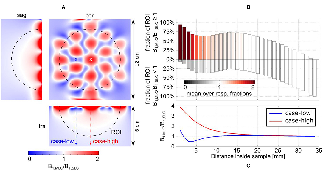
Figure 6. Detailed analysis of the transmit efficiency ratio between MLC and SLC at 3 T. (A) Ratio maps in the central sagittal and transversal slice as well as a coronal slice in a depth of 7 mm. (B) Analysis of the ratio in the ROI shown by the dashed black line in (A). The position of the bars along the y-axis shows the fractions of the ROI for which either the MLC or the SLC have higher transmit efficiency. The color of the bars indicates how much the ratio in the respective fractions deviates from 1; i.e., white indicates comparable performance (1 ± 5%). (C) Line profiles parallel to the coil axis for locations of high (red dashed line and white cross, “case-high”) and low (blue dashed line and cross, “case-low”) B1 intensity of the MLC.
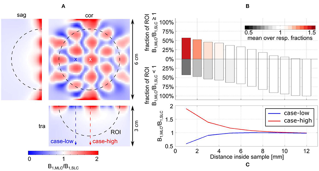
Figure 7. Detailed analysis of the transmit efficiency ratio between MLC and SLC at 7 T. (A) Ratio maps in the central sagittal and transversal slice as well as a coronal slice in a depth of 2 mm. (B) Analysis of the ratio in the ROI shown by the dashed black line in (A). The position of the bars along the y-axis shows the fractions of the ROI for which either the MLC or the SLC have higher transmit efficiency. The color of the bars indicates how much the ratio in the respective fractions deviates from 1; i.e., white indicates comparable performance (1 ± 5%). (C) Line profiles parallel to the coil axis for locations of high (red dashed line and white cross, “case-high”) and low (blue dashed line and cross, “case-low”) B1 intensity of the MLC.
A quantitative comparison of fullwave simulation and measurement results reveals that the values extracted from experimental data are ~15 and 25% lower than the simulated values for 3 T and 7 T, respectively. There are several potential reasons for this. The most plausible explanation, in our opinion, is a mismatch in sample conductivity between experiment and simulation. In simulation, the sample conductivity was fixed to the value given in the methods section, while the conductivity of the phantom solution was determined with a simple DC probe. However, the conductivity of saline solution generally increases with frequency [37]. Thus, it can be assumed that the conductivity of the phantom is higher in experiments than in simulations, which would result in a stronger dampening of the inside the sample. Another reason for the discrepancy between simulation and measurement could be an underestimation of losses, either in the coil (as it can be seen from the measured and simulated Q-values summarized in Table 2) or in the interface components.
For 3 T experiments, the patterns shown in the first slice of Figure 3 appear smeared; further, a strong edge between regions inside and outside the phantom can be observed in this slice. The reason for this is, that the walls of the phantom canister are very thin, and that, therefore, the shape of the phantom is not perfectly rectangular, but slightly curved. When the large 3 T coils with an outer diameter of 12 cm were attached to the phantom with adhesive tape, the coil PCBs were slightly bent so as to perfectly match the phantom surface. This effect is not observed on the images acquired at 7 T because the overall dimension of the 7 T coils (6 cm) is small enough to produce negligible bending when the coils were attached to the canister.
For analytical calculations, results deviate more from those obtained by the other methods. A stronger decrease of SRF with increasing distance from the coil occurs, the performance of the SLCs is clearly underestimated in comparison to the MLCs, and the left-right asymmetry depicted in fullwave simulation and measurements is not observable. This can be explained by the limitations that apply for the analytical approach. Firstly, the used equations are valid in the quasi-static domain only and, therefore, do not account for propagation effects of the RF EM field that can occur at high frequency, e.g., the proton Larmor frequency at 7 T. This explains the larger deviation observed at 7 T, especially the left-right asymmetry [38]. Secondly, for MLCs, the analytical computation was done considering small loops carrying equal current without accounting for the small conducting lines that connect the individual loops, without exactly calculating mutual resistances, and without accounting for mutual inductances between the loops that tend to reduce the magnetic efficiency; thus, the performance of the MLCs is likely overestimated in analytical calculations.
Nonetheless, the behavior, that MLCs produce a higher field than SLCs in regions close to the coil (especially directly below the small loops) expected from the rough estimation based on theoretical considerations, is well confirmed by analytical calculations, fullwave 3D simulation as well as experimental data. In regions located further away from the coil, strengths of MLCs and SLCs become comparable.
SAR
MLCs and SLCs were also compared in terms of SAR values obtained from fullwave simulation data, in order to assess the usability of MLCs in future in vivo studies regarding safety in terms of RF heating. Maximum 10 g-averaged SAR was found to be slightly lower for MLCs than for SLCs, as shown in Table 3. This is an interesting finding, especially in the regard, that lower pulse voltages are required with MLCs to generate the same flip angles as SLCs in regions close to the coil, as can be concluded from simulated and measured maps.
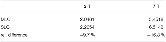
Table 3. Maximum 10 g-averaged SAR values.
SNR in MR Imaging
Figures 8, 9 show SNR maps and corresponding ratio maps obtained from 3D GRE acquisitions for MLCs and SLCs at 3 T and 7 T, respectively. A clear SNR increase can be observed for the MLCs in regions close to the coil, especially directly below the small loops. Further, it can be seen, that the lateral coverage as well as the SNR in deeper lying regions of the phantom (i.e., further away from the coil) are comparable for MLCs and SLCs.
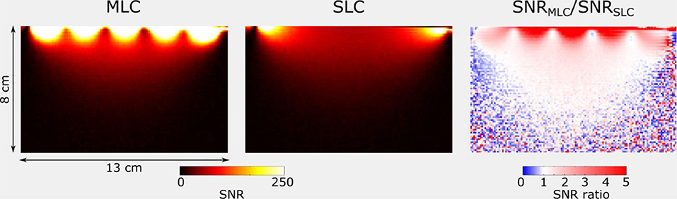
Figure 8. SNR and ratio maps obtained for the central sagittal slice of 3D GRE acquisitions at 3 T for MLC and SLC, respectively. Maps were cropped, so as to remove noise-only regions.
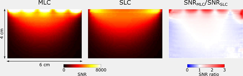
Figure 9. SNR and ratio maps obtained for the central sagittal slice of 3D GRE acquisitions at 7 T for MLC and SLC, respectively. Maps were cropped, so as to remove noise-only regions.
Discussion and Conclusion
Discussion
In this study, we have introduced the MLC principle, and we have investigated the sensitivity improvement that can be achieved in comparison to SLCs with the same overall dimensions. This comparison was done using different methods. Starting from a rough estimation, the expected gain was evaluated more precisely using analytical formulae and, finally, determined using fullwave EM simulations and MR experiments. Results from all employed methods consistently show a strong sensitivity gain with MLCs over SLCs in regions close to the coil (approximately up to the radius of the individual loops in the MLC), especially directly below the small loops, and comparable performance for regions located further away from the coil.
While in this work we have investigated MLCs composed of 19 loops with two different sizes operating at 123.2 MHz and 297.2 MHz, the obtained results are representative for the general sensitivity improvement that can be achieved by using the MLC design. Depending on the operating frequency and the desired FoV, MLCs with different number of loops or with different loop diameter or shape can also be advantageous. The highest benefit of MLCs is observed when sample induced noise dominates. As a general trend, this is the case when using surface coils larger than 3 cm in diameter and operating at static field strengths of 1.5 T and above, i.e., for most of the common settings encountered in clinical MRI applications. It should be noted that the sensitivity improvement achievable with increasing the number of small loops is limited by noise correlation. This limit will be reached when the total sample related resistance will be more increased due to noise correlation than the sample noise reduction achieved by using smaller loops in series (). As a perspective, for configurations where the use of small loops in series is advantageous in the presence of noise correlation, even higher SNR improvement could be obtained by minimizing noise correlation; for instance, Algarin et al. [39] have recently demonstrated a significant reduction of the electrical coupling coefficient using a metamaterial surface.
Results presented here were obtained using MLCs fabricated from copper clad laminated FR4 substrate, but the MLC principle shows no particular restriction regarding the technology used for coil fabrication and can therefore be applied as well to produce MLCs made of flexible substrates or, more standardly, from wound copper wire.
As compared to the rough estimate of the sensitivity improvement presented in section Rough estimate of the sensitivity improvement expected with MLCs, the RF sensitivity factor computation based on analytical formulae provides a more accurate evaluation and allows for a rapid computation of 3D sensitivity maps that are informative and useful for the MLC design optimization step. However, some limitations apply for this approach as described above; therefore, the use of more advanced simulation methods and the final experimental evaluation are indispensable for RF coil development and evaluation at high and ultra-high field strength.
As it can be observed in sensitivity maps, at very short distances inside the sample, i.e., comparable to the diameters of the individual loops of the MLC, signal loss occurs between adjacent loops of the MLC because of the reverse direction of the field created in this region and because of MR-inefficient B1 components parallel to B0. While this phenomenon vanishes further away inside the sample, it might be problematic for MR applications targeting surface ROIs such as skin imaging. The simplest solution in this case would be to offset the coil slightly from the sample in a way to still benefit from the (smaller) SNR gain, but strongly reduce the inhomogeneity. To remedy this issue without offsetting the coil, more complex MLC designs will be investigated in future work so as to achieve current patterns that generate a more uniform B1 distribution close to the coil. For instance, this could be done by adding smaller loops in series to the initial ones in the regions where signal loss occurs. This approach is possible as the MLC principle brings additional degrees of freedom for coil design as compared to SLCs, which potentially enables the realization of specific coil patterns with respect to the sample shape, but also the optimization of the homogeneity of the detection sensitivity in a target region inside the sample.
Several MRI applications may well benefit from MLCs, which will be primarily used as single coils for applications requiring high sensitivity over a FoV that is large compared to the target depth, e.g., skin imaging [40], or ex vivo imaging of brain slices [41]. In addition, MLCs can also be employed as building block of an array when an even larger FoV has to be covered. The detailed investigation of MLC arrays is subject to future studies.
As compared to arrays of SLCs, the MLC principle brings simplicity for both, the design and the fabrication, while aiming at achieving a comparable performance in terms of sensitivity. This renders possible a significant cost reduction that may strongly inure to the benefit of developing countries where very high-priced parallel acquisition MRI systems appear unaffordable. On the other hand, using a single MLC instead of an array of SLCs is not compatible with parallel imaging approaches for accelerated image acquisition and does not allow for SNR optimization using a weighted signal combination of the individual channels. However, for those applications expected to benefit most from the MLC principle, targeting very high resolution in shallow depth over a large FoV, sensitivity is typically more important than acquisition speed.
Conclusion
In this paper, the proof of concept of a novel RF coil design, the multi-loop coil design, has been established. The MLC concept exploits the intrinsically high sensitivity of small surface coils that achieve strong magnetic coupling to the sample while reducing the sample induced noise, together with achieving a large FoV by associating multiple small loops in series. It allows for significant sensitivity improvement when the sample induced noise dominates over the internal coil noise, relevant for most clinically applied surface coils (>3 cm diameter, ≥ 1.5 T).
As a general tendency, close to the coil plane, the MLC design potentially achieves higher RF sensitivity as compared to a single loop coil having the same lateral size. Maximum gains in transmit efficiency by a factor between 2 and 4 were obtained experimentally depending on the field strength and coil size. At long distance from the coil, as the induction coefficients of the individual loops of the MLC are summed up, the achieved sensitivity is comparable to that of the equivalent SLC.
Data Availability Statement
The datasets generated for this study are available on request to the corresponding author.
Author Contributions
J-CG, EL, and RF-K planned the study. J-CG and MP-Q performed the analytical calculation. SH and RF-K performed the fullwave simulations. RF-K acquired the experimental data and performed the data analysis. All authors contributed to writing and proof-reading the article.
Funding
This work was funded by the Austrian/French OeAD WTZ grant FR 03/2018 and the Austrian Science Fund grant FWF P28059.
Conflict of Interest
The authors declare that the research was conducted in the absence of any commercial or financial relationships that could be construed as a potential conflict of interest.
Acknowledgments
The authors thank Ms. Anika Franta and Ms. Hannah Goetz for contributing to this work.
References
1. Darrasse L, Ginefri JC. Perspectives with cryogenic RF probes in biomedical MRI. Biochimie. (2003) 85:915–37. doi: 10.1016/j.biochi.2003.09.016
2. Redpath TW. Signal-to-noise ratio in MRI. Br J Radiol. (1998) 71:704–7. doi: 10.1259/bjr.71.847.9771379
3. Kneeland JB, Hyde JS. High-resolution MR imaging with local coils. Radiology. (1989) 171:1–7. doi: 10.1148/radiology.171.1.2648466
4. Ackerman JJH, Grove TH, Wong GG, Gadian DG, Radda GK. Mapping of metabolites in whole animals by 31P NMR using surface coils. Nature. (1980) 283:167–70. doi: 10.1038/283167a0
5. Bittoun J, Saint-Jalmes H, Querleux BG, Darrasse L, Jolivet O, Peretti II, et al. In vivo high-resolution MR imaging of the skin in a whole-body system at 1.5 T. Radiology. (1990) 176:457–60. doi: 10.1148/radiology.176.2.2367660
6. Roemer PB, Edelstein WA, Hayes CE, Souza SP, Mueller OM. The NMR phased array. Magn Reson Med. (1990) 16:192–225. doi: 10.1002/mrm.1910160203
7. Pruessmann KP, Weiger M, Scheidegger MB, Boesiger P. SENSE: sensitivity encoding for fast MRI. Magn Reson Med. (1999) 42:952–62. doi: 10.1002/(SICI)1522-2594(199911)42:5<952::AID-MRM16>3.0.CO;2-S
8. Sodickson DK, Manning WJ. Simultaneous acquisition of spatial harmonics (SMASH): fast imaging with radiofrequency coil arrays. Magn Reson Med. (1997) 38:591–603. doi: 10.1002/mrm.1910380414
9. Heidemann RM, Ozsarlak O, Parizel PM, Michiels J, Kiefer B, Jellus V, et al. A brief review of parallel magnetic resonance imaging. Eur Radiol. (2003) 13:2323–37. doi: 10.1007/s00330-003-1992-7
10. Ohliger MA, Sodickson DK. An introduction to coil array design for parallel MRI. NMR Biomed. (2006) 19:300–15. doi: 10.1002/nbm.1046
11. Dona Lemus OM, Konyer NB, Noseworthy MD. Micro-strip surface coils using fractal geometry for 129Xe lung imaging applications. In: Proceedings of the International Society for Magnetic Resonance in Medicine. Paris (2018). p. 1713.
12. Mansfield P. The petal resonator: a new approach to surface coil design for NMR imaging and spectroscopy. J Phys D Appl Phys. (1988) 21:1643–4. doi: 10.1088/0022-3727/21/11/015
13. Rodriguez AO, Hidalgo SS, Rojas R, Barrios FA. Experimental development of a petal resonator surface coil. Magn Reson Imaging. (2005) 23:1027–33. doi: 10.1016/j.mri.2005.09.001
14. Robitaille PM, Berliner L. Ultra High Field Magnetic Resonance Imaging. Boston, MA: Springer (2006). doi: 10.1007/978-0-387-49648-1
15. Simpson J, Lane J, Immer C, Youngquist R. Simple Analytic Expressions for the Magnetic Field of a Circular Current Loop. (2001). Available online at: https://ntrs.nasa.gov/archive/nasa/casi.ntrs.nasa.gov/20010038494.pdf (accessed September 10, 2019).
16. Hoult DI, Lauterbur PC. The sensitivity of the zeugmatographic experiment involving human samples. J Magn Reson. (1979) 34:425–33. doi: 10.1016/0022-2364(79)90019-2
17. Decorps M, Blondet P, Reutenauer H, Albrand JP, Remy C. An inductively coupled, series-tuned NMR probe. J Magn Reson. (1985) 65:100–9. doi: 10.1016/0022-2364(85)90378-6
18. Guéron M, Leroy JL. NMR of water protons. The detection of their nuclear-spin noise, and a simple determination of absolute probe sensitivity based on radiation damping. J Magn Reson. (1989) 85:209–15. doi: 10.1016/0022-2364(89)90338-7
19. Kraichman M. Impedance of a circular loop in an infinite conducting medium. J Res Nat Bur Stand D Radio Propag. (1962) 66D:499–503. doi: 10.6028/jres.066D.050
20. Suits BH, Garroway AN, Miller JB. Surface and gradiometer coils near a conducting body: the lift-off effect. J Magn Reson. (1998) 135:373–9. doi: 10.1006/jmre.1998.1608
21. Serfaty S, Darrasse L, Kan S. The pinpoint NMR coil. In: Proceedings of the SMR Second Annual Meeting. San Francisco, CA (1994). p. 219.
22. Werner DH. An exact integration procedure for vector potentials of thin circular loop antennas. IEEE Trans Antennas Propag. (1996) 44:157–65. doi: 10.1109/8.481642
23. Kumar A, Edelstein WA, Bottomley PA. Noise figure limits for circular loop MR coils. Magn Reson Med. (2009) 61:1201–9. doi: 10.1002/mrm.21948
24. Giovannetti G, Tiberi G. Skin effect estimation in radiofrequency coils for nuclear magnetic resonance applications. Appl Magn Reson. (2016) 47:601–12. doi: 10.1007/s00723-016-0780-x
25. Giovannetti G, Hartwig V, Landini L, Santarelli MF. Classical and lateral skin effect contributions estimation in strip MR coils. Concepts Magn Reson B Magn Reson Eng. (2012) 41B:57–61. doi: 10.1002/cmr.b.21210
27. Terman FE. Radio Engineers' Handbook. 1st Ed. New York, NY: McGraw-Hill Book Company, Inc. (1943).
28. Gonord P, Kan S, Leroy-Willig A. Parallel-plate split-conductor surface coil: analysis and design. Magn Reson Med. (1988) 6:353–8. doi: 10.1002/mrm.1910060313
29. Yee KS. Numerical solution of initial boundary value problems involving Maxwell's equations in isotropic media. IEEE Trans Antennas Propag. (1966) 14:302–7. doi: 10.1109/TAP.1966.1138693
30. Kozlov M, Turner R. Fast MRI coil analysis based on 3-D electromagnetic and RF circuit co-simulation. J Magn Reson. (2009) 200:147–52. doi: 10.1016/j.jmr.2009.06.005
31. Lemdiasov RA, Obi AA, Ludwig R. A numerical postprocessing procedure for analyzing radio frequency MRI coils. Concepts Magn Reson A Magn Reson Eng. (2011) 38A:133–47. doi: 10.1002/cmr.a.20217
32. Graesslin I, Homann H, Biederer S, Börnert P, Nehrke K, Vernickel P, et al. A specific absorption rate prediction concept for parallel transmission MR. Magn Reson Med. (2012) 68:1664–74. doi: 10.1002/mrm.24138
33. Kuehne A, Goluch S, Waxmann P, Seifert F, Ittermann B, Moser E, et al. Power balance and loss mechanism analysis in RF transmit coil arrays. Magn Reson Med. (2015) 74:1165–76. doi: 10.1002/mrm.25493
34. Ginefri JC, Durand E, Darrasse L. Quick measurement of nuclear magnetic resonance coil sensitivity with a single-loop probe. Rev Sci Instrum. (1999) 70:4730–1. doi: 10.1063/1.1150142
35. Chung S, Kim D, Breton E, Axel L. Rapid B1+ mapping using a preconditioning RF pulse with TurboFLASH readout. Magn Reson Med. (2010) 64:439–46. doi: 10.1002/mrm.22423
36. Pohmann R, Scheffler K. A theoretical and experimental comparison of different techniques for B1 mapping at very high fields. NMR Biomed. (2013) 26:265–75. doi: 10.1002/nbm.2844
37. Giovannetti G, Frijia F, Menichetti L, Hartwig V, Viti V, Landini L. An efficient method for electrical conductivity measurement in the RF range. Concepts Magn Reson B Magn Reson Eng. (2010) 37B:160–6. doi: 10.1002/cmr.b.20165
38. Collins CM, Wang Z. Calculation of radiofrequency electromagnetic fields and their effects in MRI of human subjects. Magn Reson Med. (2011) 65:1470–82. doi: 10.1002/mrm.22845
39. Algarin JM, Breuer F, Behr VC, Freire MJ. Analysis of the noise correlation in MRI coil arrays loaded with metamaterial magnetoinductive lenses. IEEE Trans Med Imaging. (2015) 34:1148–54. doi: 10.1109/TMI.2014.2377792
40. Laistler E, Loewe R, Moser E. Magnetic resonance microimaging of human skin vasculature in vivo at 3 Tesla. Magn Reson Med. (2011) 65:1718–23. doi: 10.1002/mrm.22743
Keywords: magnetic resonance imaging, radio frequency coil, surface coil, electromagnetic simulation, B1 mapping
Citation: Frass-Kriegl R, Hosseinnezhadian S, Poirier-Quinot M, Laistler E and Ginefri J-C (2020) Multi-Loop Radio Frequency Coil Elements for Magnetic Resonance Imaging: Theory, Simulation, and Experimental Investigation. Front. Phys. 7:237. doi: 10.3389/fphy.2019.00237
Received: 27 September 2019; Accepted: 16 December 2019;
Published: 15 January 2020.
Edited by:
Simo Saarakkala, University of Oulu, FinlandReviewed by:
Stephan Orzada, University of Duisburg-Essen, GermanyAndre Kuehne, MRI.TOOLS GmbH, Germany
Copyright © 2020 Frass-Kriegl, Hosseinnezhadian, Poirier-Quinot, Laistler and Ginefri. This is an open-access article distributed under the terms of the Creative Commons Attribution License (CC BY). The use, distribution or reproduction in other forums is permitted, provided the original author(s) and the copyright owner(s) are credited and that the original publication in this journal is cited, in accordance with accepted academic practice. No use, distribution or reproduction is permitted which does not comply with these terms.
*Correspondence: Jean-Christophe Ginefri, jean-christophe.ginefri@u-psud.fr