Tilted Snowplow Ponderomotive Electron Acceleration With Spatio-Temporally Shaped Ultrafast Laser Pulses

1. Introduction

One of the issues facing the use of laser pulses to accelerate electrons is the relative difference in the velocity of the electrons and of the light wave. For direct field acceleration, injected electrons must be close to the phase velocity, while for wakefield acceleration and ponderomotive acceleration, it is the pulse group velocity relative to the electron velocity that is relevant. Typically the phase and group velocities are at or close to the speed of light, and fast electrons must be injected, and timed with the pulse. Spatio-temporal shaping of the pulses offers a route toward controlling the pulse group velocity over a wide range. In recent years, several groups have been pursuing the use of spatial chirp, the ordering of the pulse frequency components in position or angle, to control the spatio-temporal intensity to slow down the effective group velocity of the wave. Angular spatial chirp produces a pulse front tilt that presents unique opportunities to study and control electron dynamics, since the effective pulse velocity can be decreased substantially below the vacuum speed of light (c).

Tilted pulses have been applied in several areas of non-linear optics and laser-matter interactions. Control of the angular dispersion has been used to match pulse fronts in second harmonic generation of broadband pulses in thick non-linear crystals [1] and for optical parametric amplification [2]. Similarly, other groups have used tilted pulses in lithium niobate to obtain high energy THz pulses [3]. The spatially-dependent arrival time of a tilted pulse can also be used for traveling-wave pumping of an x-ray laser in an ablating plasma (e.g., [4]). The tilted pulse has also been shown to result in interesting asymmetric structures during micromachining on surfaces [5, 6]. When a pulse is focused with angular chirp, the intensity is localized along the optical axis due to simultaneous spatial and temporal focusing (SSTF) [7, 8]. This intensity localization is extremely useful for micromachining [9, 10] and laser surgery [11].

One of the primary mechanisms for a laser beam to couple to plasmas is the ponderomotive force. The optical pressure drives lighter electrons away from regions of high intensity. For relativistic intensities (where the average oscillation energy of the electron in the field is comparable to its rest mass), the ponderomotive force can drive most or all of the electrons out of the focal region, leaving a wakefield behind the pulse that can be used to accelerate electrons [12]. In this paper, we propose to use tilted laser pulses, like a snowplow, to knock the electrons out of the focus to one side. By slowing down the effective velocity of the pulse we predict that the intensity required to drive the electrons out is dramatically reduced compared to using a conventionally-focused beam. In this paper, we consider the acceleration at densities sufficiently low that space charge is not a factor; in later work we will consider higher densities, including the wakefield regime. While it is beyond the scope of this initial paper to fully evaluate this scheme for applications, an ultrafast source of moderate energy electron pulses can have application to ultrafast electron diffraction [13], generation of coherent light, and injection into wakefield accelerators.

Before presenting the details, we illustrate the acceleration scheme in Figure 1, which shows a simulation of the process using the particle-in-cell code OSIRIS 4.0 [14, 15]. In the top left frame, the tilted pulse (orange) is about to meet a stationary electron bunch at the origin (blue). As the pulse propagates to the right, the electron bunch is accelerated in the direction of the tilted intensity gradient. Because the effective interaction velocity along this direction is slower than c, the electron bunch is captured and accelerated. In section 2, we provide a brief overview of the optics of tilted pulses. In section 3, the simple non-relativistic theory of tilted pulse acceleration is presented, followed by the relativistic theory and modeling in section 4. Finally, in section 5, we offer a summary and conclusion.

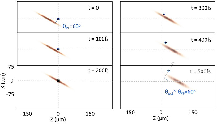
Figure 1. Calculation in the lab frame from the OSIRIS 4.0 PIC code for a 20 fs pulse duration, 60° PFT angle, and 200 keV peak ponderomotive potential. The red shows the intensity distribution for the tilted pulse fronts. The blue-black dots represent the location of the electron bunch [2.5 μm square, initial position (X₀, Z₀) = (0, 0)]. Here the focal plane is at Z = −20μm. The horizontal dashed lines represent the optical axis for each of the frames. The arrow at t = 500fs represents the direction of the accelerated bunch, which is close to the normal of the pulse front.

2. Generation of Tilted Pulses With Angular Spatial Chirp

In ultrafast laser systems, care is typically taken to ensure that all of the spectral components of the beam are spatially overlapped. However, in the past several years, more researchers have been seeking to exploit special properties of beams that have spatial chirp, where one or more of the beam parameters vary across the spectrum. For example, a beam with transverse spatial chirp exhibits the "lighthouse" effect, where the wavefront angle is a function of time. This effect has lead to the production of angularly separated attosecond pulses through high order harmonic generation [16]. Angular spatial chirp leads to a complementary effect, known as simultaneous spatial and temporal focusing (SSTF). These beams have unique properties that can be exploited to control and manipulate non-linear optical processes. SSTF leads to a localization of the intensity along the optical axis that is especially useful for micromachining [6, 10] and laser surgery [11], as well as non-linear microscopy [17, 18].

While the details of the spatio-temporal structure of these pulses can be found elsewhere [19], there are several features of these tilted pulses that are relevant to the current discussion. A simple understanding of temporal focusing and pulse front tilt can be obtained by considering a group of plane waves crossing at Z = 0 where the propagation angle (θ) relative to the Z−axis depends on frequency ω. The central frequency component ω₀ is defined to be along the Z−axis, so that θ(ω₀) = 0. In the spatial-spectral domain, this beam can be written as $E_{0}exp\left[-{(\omega -{\omega }_0)}^2/\Delta {\omega }^2\right]exp\left[i(\omega /c)(Xsin(\theta (\omega ))+Zcos(\theta (\omega )))\right]$, where E₀ is the electric field amplitude and Δω is the spectral bandwidth. Derivatives of the spectral phase φ(X, Z, ω) = (ω/c)(X sin θ(ω) + Z cos θ(ω)) lead to an understanding of the spatio-temporal properties of the beam. Along the Z−axis, the group delay dispersion, ${\phi }_2(Z)={\partial }_{\omega }^2(\omega Zcos\theta )/c{|}_{{\omega }_0}$ leads to a pulse that is fully compressed only at Z = 0. This longitudinal compression combines with the focusing and the spectral overlap to give a shorter depth of focus than would be expected for a conventionally focused beam of the same spot radius.

Along with intensity localization, the angular chirp leads to a strong pulse front tilt (PFT). At Z = 0, we can find the arrival time of the pulse by calculating the group delay: φ₁(X) = ∂_ωφ|_ω0 = ∂_ωθ|_ω0Xω₀/c. The pulse arrives earliest for X < 0, and the pulse sweeps across the target Z = 0 plane with a velocity v_xPF = X/φ₁(X). Noting that the pulse travels at a speed c in the Z direction, the pulse is seen to have a tilt in the pulse front with an angle given by tan(θ_PF) = c/v_xPF, where θ_PF = 0 when there is no PFT.

PFT control has been applied in previous work in non-linear optics such as THz generation in crystals [3], non-collinear optical parametric amplification (e.g., [20]) and achromatic phase matching [1]. In these examples the group velocity control makes the non-linear processes more efficient. PFT has also been exploited in traveling-wave pumping of x-ray lasers (e.g., [4]).

Spatially-chirped pulses can be made by converting the standard double pass pulse compressor to single pass by increasing the separation of the diffraction gratings by a factor of two. Normally, the separation of the gratings is fixed to optimize pulse compression, but we have shown a pulse compressor that allows us to vary the degree of spatial chirp while maintaining optimal pulse compression [21]. Rather than using a single pass compressor, the beam passes through the grating pair twice, but with a grating separation that is longer for one pass compared to the other. Our current design allows us to tune the PFT from zero all the way to ${\theta }_{PF}<88^{°}$.

3. Non-relativistic Single Particle Theory

The essential concepts behind the tilted pulse acceleration scheme can be most easily illustrated by considering acceleration in the non-relativistic limit. For simplicity, we will consider a tilted pulse propagating in the Z−direction with a tilt angle θ_PF where we also neglect limits on the transverse width of the beam. This non-physical idealized framework will serve as a reference to which more complete calculations can be compared.

An approximate form for the envelope of the pulse intensity, I, as

Here, I₀ is the peak intensity, and τ is the pulse duration. While this simple representation of a tilted pulse does not capture the full spatio-temporal evolution of the intensity through the focus, we will use it for conveying the essential dynamics of tilted pulse acceleration. We have developed an analytic expression for the evolution of the spatio-temporal pulse intensity following the method outlined in an earlier paper [18], and we find that the approximation of Equation (1) is best for electrons starting near the focal plane (Z = 0). Three dimensional effects will be discussed later in the paper.

The common definition of the non-relativistic ponderomotive potential is the cycle-averaged quiver energy of a free electron in an electromagnetic wave:

where e is the electron charge, E₀ is the electric field amplitude, m_e is the electron rest mass, r_e is the classical electron radius, λ is the laser wavelength, and I is the time-averaged beam intensity. In the non-relativistic limit, we can calculate the force on an electron from F = −∇U_p. Equation (2) can be derived from the linearized equations of motion of a single charged particle in the Lorentz force of a high-frequency electromagnetic field [22]. The force comes out of equations of motion for the guiding center of the fast oscillations of the particle. A more general form of the ponderomotive force can be derived through Vlasov theory that includes interactions with particles that are resonant with the field [23]. Another approach using the stress tensor and fluid theory addresses the time-dependent force that emerges from the longitudinal gradients of the field [24]. At relativistic intensities, the trajectories of the electron become anharmonic, and approximate forms of the ponderomotive force must be derived that account for the relativistic mass increase. In a later section we will use the approximation developed by Mora and Antonsen [25]. Owing to the complicated nature of these approximations, full-field calculations that do not rely on the ponderomotive approximations can be used to verify that the results of the simpler theory hold up. For this we turn to the particle-in-cell calculations that include the fast electron oscillations.

In the non-relativistic limit, we can calculate the force on an electron from F = −∇U_p, obtaining:

where U_P0 is the peak ponderomotive potential. By looking at the vector components of Equation (3), we can see that with a simple rotation of the reference frame we can align the force along a z′ axis that is normal to the pulse front. In this rotated frame, the laser pulse has a ponderomotive potential that is traveling at a reduced speed v_PF = c cos θ_PF:

Now consider a reference frame that is moving in the z′ direction at the pulse front velocity. If an electron is at rest in the lab frame, then it is moving toward the pulse front with velocity −c cos(θ_PF) in the moving frame. Upon reflection from the potential, the velocity changes to +c cos(θ_PF). Therefore, from simple energy considerations, the electron will be “reflected” from this potential hill if the peak ponderomotive potential is greater than the capture threshold:

where the superscript “cap0” reminds the reader that the initial electron velocity is zero.

Now suppose the electron has an initial velocity in the lab frame v₀, where v₀ > 0 corresponds to an electron moving in the same direction as the pulse front in the rotated lab frame, i.e., along the z′ axis. In the moving frame, the electron approaches the stationary potential at the speed −(c cos(θ_PF) − v₀) leading to a new capture threshold:

It is important to note that with strong angular chirp approaching the laser focus it is straightforward to produce pulse front angles as large as ${\theta }_{PF}=88^{°}$. In such cases, capture can take place with a ponderomotive potential that is approximately 3 orders of magnitude less than the electron rest mass energy.

When the electron is captured and accelerated (reflected in the moving frame), the reversal of the electron velocity in the moving frame corresponds to a net acceleration in the lab frame to a velocity of 2c cos(θ_PF) − v₀, or an output kinetic energy of

Here the minus sign is taken if v₀ > 0, which corresponds to a seed electron velocity in the same direction as the pulse front. Note that even if $U_{P0}>U_P^{cap}$, the output energy is determined only by the pulse front velocity (v_PF) and the seed electron energy (v₀), not the value of U_P0. If v₀ = 0, $K{E}_{out}=4U_P^{cap0}$. We will see later how a finite beam size affects this result.

In the first form of Equation (7), we see that the output kinetic energy is smaller if the initial direction is co-moving with the pulse (v₀ > 0) compared to if it is moving into the pulse (v₀ < 0). This is perhaps counter-intuitive, but consider the situation in the pulse frame. If the particle is initially at rest in the lab frame, the change in momentum after reflection is 2m_ev_PF. Any additional momentum toward the pulse front will increase the momentum transfer, while if the particle is initially moving in the same direction as the pulse front in the lab frame, the momentum increase from the interaction is lower since the relative velocities are smaller. This is similar to the situation in American baseball, where the batter can hit the ball farther off a fast ball than if the ball is hit off a tee (i.e., starting from rest). One might conclude from this that if electrons are injected into the field, it is best to seed the electrons in the direction opposite the pulse front. However, this is only true if the pulse intensity is sufficient to reflect the electrons, i.e., $U_{P0}>U_P^{cap}(v_0)$. Since the capture threshold, Equation (6), is higher for v₀ < 0, we can consider whether a combination of smaller tilt angle and co-moving injection would be a more efficient acceleration scheme.

If the available input intensity is fixed, and we have the ability to seed the acceleration with electrons, we can adjust θ_PF so that $U_{P0}\ge U_P^{cap}(v_0)$. We can then calculate the KE that is added to the input KE: ΔKE_out = KE_out − KE_in, assuming the tilt angle is always adjusted so that $U_{P0}=U_P^{cap}$ as v₀ is varied. Using Equation (6) to solve for cos(θ_PF), we find that

Here the upper sign is taken for co-moving injection (v₀ > 0). As an example, suppose we accelerate an electron bunch from rest using a peak ponderomotive potential of U_P0 and the angle is adjusted to be at the capture threshold ($U_{P0}=U_P^{cap0}$). Then, the electrons of kinetic energy 4U_P0 are injected into a second stage with a pulse of the same intensity, and θ_PF for this stage is adjusted to be at the threshold for capture. At the end, KE_out = 12U_P0, which is 1.5x higher than if all the energy were put into a single stage. For a fixed total energy, the optimum fraction of energy to use in the first stage is just above 0.25, which yields an improvement of 1.62x over the single stage case. We will see in section 4.1 that when the initial electron velocity is near zero, variations in the output kinetic energy are very sensitive to input energy perturbations, however, when the acceleration is seeded with some average initial velocity, this sensitivity is dramatically reduced.

Although the force is only in the direction normal to the pulse front, there is motion along the pulse front at the speed $v_x^{\prime }=csin({\theta }_{PF})$. Of course in this ideal case of infinite transverse width, this motion has no bearing on the kinematics. For a finite beam width however, there will be some electrons that will slide off the pulse front before being fully accelerated. We can estimate the time, ΔT, the electron is accelerated by the pulse by considering an infinite width (in X) beam with a triangular temporal profile and a duration of τ_tri from peak to toe. Here, the force is constant, and since the momentum change is 2m_ec cos(θ_PF), then ΔT = 4τ_tri/r_Up, where $r_{Up}=U_{P0}/U_P^{cap0}$ is the measure of how far the focused intensity is above the capture threshold. The acceleration time is shorter for shorter pulses and larger r_Up. The distance the electron travels in the rotated frame in the x′ direction is $\Delta x^{\prime }=c\Delta Tcos({\theta }_{PF})$. To get the transverse displacement in the un-rotated X direction, we integrate the equation of motion in the z′ direction, then rotate back to obtain $\Delta X\mathrm{\text{=}}\frac{\mathrm{\text{2c}}\tau }{r_{U\mathrm{\text{p}}}}sin(\mathrm{\text{2}}{\theta }_{\mathrm{\text{pf}}})\left({(1+\frac{r_{U\mathrm{\text{p}}}}{\mathrm{\text{4}}})}^{\mathrm{\text{2}}}\mathrm{\text{+ 1}}\right)$. For ${\theta }_{PF}=60^{°}$, τ_tri = 20fs, and r_Up = 2, the focused spot diameter must be a minimum of ΔX = 17μm. However, for a steeper angle, ${\theta }_{PF}=85^{°}$, ΔX = 3.4μm, which is considerably smaller.

Finally, we note that in the stationary lab frame (Z, X) the output velocity vector is $\left\{v_z,v_x\right\}=\left\{2c{cos}^2({\theta }_{PF}),csin(2{\theta }_{PF})\right\}$ and the output angle (${tan}^{-1}(v_x/v_z)$) is simply in the direction of the normal to the pulse front, consistent with the direction of the applied force.

Several very important observations come from this simple analysis. First, all electrons will be captured, provide the capture condition is satisfied. Second, the output kinetic energy is dependent only on the PFT angle, not on the intensity of the laser. Therefore, even when the laser pulse has a transverse intensity profile, the electrons that are fully captured will have the same output energy. These two properties of the tilted pulse acceleration scheme show promise for creating an electron bunch with high brightness. The analysis later in this paper will explore the robustness of the scheme, accounting for the effects of relativity and the non-constant transverse intensity profile.

4. Relativistic Single-Particle Analysis of Tilted Pulse Acceleration

4.1. One Dimensional Analysis With Infinite Width Tilted Pulse

While the non-relativistic calculation is extremely useful for illustrating the concept of tilted pulse ponderomotive acceleration, the accelerated electrons will exhibit relativistic effects even for modest laser pulse intensities. Mora and Antonsen [25] give an expression for the relativistic ponderomotive force, written in the lab frame:

where the cycle-average relativistic factor is

In these expressions, $\bar{p}$ is the cycle-averaged momentum. From Equation (9), we see that in the high-intensity limit, the force increases only as the square-root of the laser intensity. The force also decreases with increasing electron momentum. While this indicates that ponderomotive acceleration is less effective for strongly relativistic velocities, we will see that it remains promising as an injection source for another acceleration stage, such as wakefield acceleration.

The direction of the force in Equation (9) is the same as the non-relativistic case. This allows us to consider the relativistic modifications to the one-dimensional non-relativistic analysis described in section 3. Since the force is non-linear, we numerically integrate the equations of motion in the lab frame using the idealized tilted pulse shown in Equation (1) to obtain the electron trajectories. Figure 2A shows electron trajectories for a fixed pulse front angle and several values of the peak ponderomotive potential, U_P0. Figure 2B shows the time-dependence of the kinetic energy, $m_e{c}^2(\gamma -1)$. For high U_P0 (blue curve) the electron is accelerated to approximately 700 keV, but when U_P0 is much less than the capture threshold (purple curve), the pulse passes by the electron without accelerating. For this low U_P0 case, the kinetic energy follows the ponderomotive potential. As U_P0 increases to just below threshold (red curve), the electron is not captured, but is shifted forward as the pulse passes by. Just above the threshold for capture (green curve), the electron rides along the top of the pulse before being accelerated in front.

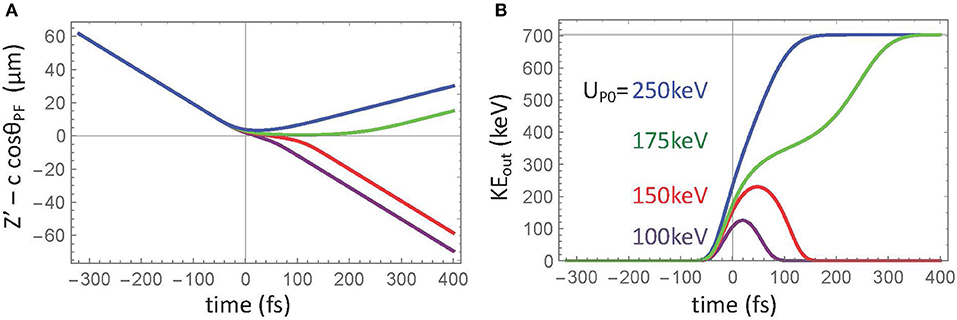
Figure 2. Relativistic calculations of acceleration in the moving frame for a pulse front angle of 50°, for which the non-relativistic capture potential is $U_P^{cap0}=100$ keV. The electron is initially at rest in the lab frame. The different curves correspond to varying values of the peak ponderomotive potential. (A) Electron trajectories and (B) kinetic energy. The horizontal gray line in (B) represents 4x the calculated threshold for capture.

We can see that in this case of infinite beam width, the final output kinetic energy is not affected by the height of the ponderomotive potential: both the blue and green curves in Figure 2 reach the same maximum value. Rather, the output kinetic energy is determined by the PFT angle, as seen in Figure 3. Below threshold, it is seen that the curves for the output energies lie on top of each other up to the threshold for capture.

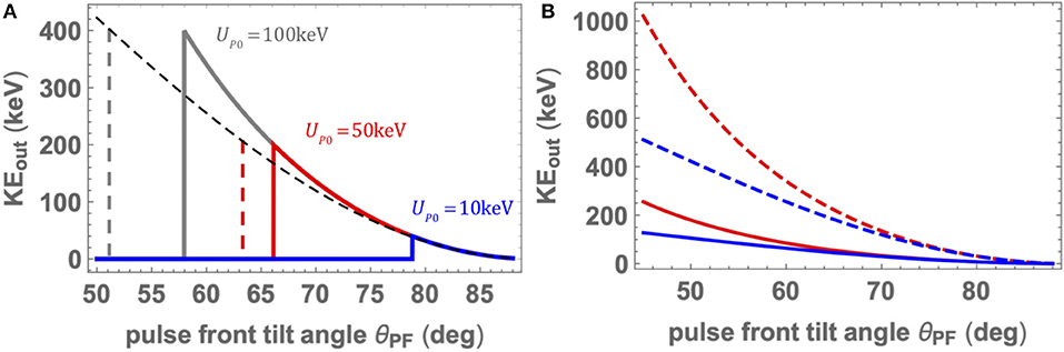
Figure 3. (A) Output kinetic energy as a function of the PFT angle for several fixed values of peak ponderomotive potential. The dashed curve shows the non-relativistic capture threshold. The vertical dashed lines represent the capture threshold angle in the non-relativistic approximation. (B) Threshold ponderomotive potential (solid) and output kinetic energy (dashed) as a function of PFT angle. The color of the curves correspond to the non-relativistic (blue) and relativistic (red) predictions.

The non-relativistic calculation for the threshold for capture (from Equation 6) is shown as a dashed curve in Figure 3A. We can see that the relativistic capture threshold is higher than the non-relativistic prediction (Equation 5). As the relativistic mass increases with higher intensity, the ponderomotive force decreases and a higher capture threshold results. The output kinetic energy at threshold is equal to four times the threshold potential for capture.

To numerically find the threshold ponderomotive potential, we iterate on the peak ponderomotive potential, calculate the trajectory, and look at the sign of $z^{\prime }(t_{max})-ccos({\theta }_{PF})t_{max}$ (as seen in Figure 2A) to see if the electron has been accelerated. We can then calculate the final kinetic energy at the maximum time of integration, t_max, when the electron has moved off of the pulse. Figure 3B shows the variation of the capture threshold as a function of PFT angle (solid lines). The blue curve shows the non-relativistic prediction, while the red curve shows the numerically calculated relativistic threshold.

The dashed lines in Figure 3B show the output kinetic energy after acceleration. In blue is the non-relativistic prediction, which is four times the capture potential shown in Equation (6). The red dashed curve results from the relativistic numerical integration and is equal to four times the relativistic capture potential. While the potential for capture is larger in the relativistic case than the non-relativistic prediction, the final kinetic energy is still four times the threshold potential. Given that the PFT angle can be tuned to ensure capture, there is no loss in effectiveness of the ponderomotive acceleration at relativistic intensity.

Next we consider the dependence of the output kinetic energy on the input kinetic energy of the electron. When there is initial electron velocity, for a given value of U_P0, the seed electron can be injected either along the direction of the pulse front normal or against it. Equation (6) shows that the capture potential is lower when a seed electron is co-moving with the pulse front, and higher if it is moving toward the pulse front. Figure 4A shows how the output kinetic energy (KE_out) depends on the seed kinetic energy (KE_in). The energies are ratioed against the capture potential $U_P^{cap0}$ at zero initial velocity; at KE_in = 0, we see the factor of four predicted above. When the seed electron is injected against the pulse front direction (KE_in < 0 in the plot), the output kinetic energy is actually higher than if the electron starts at rest or is injected in the same direction as the pulse front (see Figure 4A). This is similar to how a baseball player can hit the ball farther off a faster pitch. The sharp cutoff for negative KE_in is at the capture threshold for the ponderomotive potential chosen for this calculation. Although seeding against the pulse front leads to higher KE_out, this approach will work only if the pulse has high enough U_P0 so that the electron is actually captured.

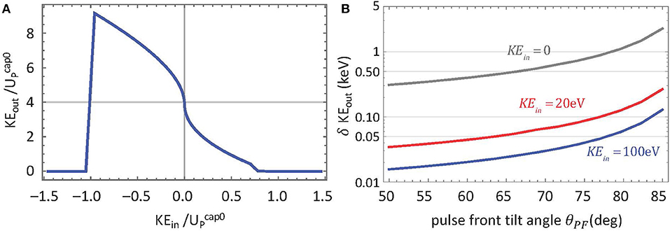
Figure 4. (A) Output kinetic energy KE_out as a function of the seed electron kinetic energy KE_in for U_P0 = 500 keV. Both energies are calculated relative to the zero initial velocity capture potential. Negative KE_in corresponds to electron velocity that is initially heading toward the beam. (B) Relative variation in the output kinetic energy as a function of PFT angle for three values of the co-moving seed kinetic energy. The test value of δKE_in is 1 eV.

The maximum energy extraction for a fixed peak intensity can be obtained if the pulse front angle can be adjusted so that the electrons are just captured. In contrast to Equation (7) where the tilt angle was held constant while KE_in was varied, consider a case where the tilt angle is adjusted to be at the capture threshold. In the non-relativistic limit, the output kinetic energy is then

The negative sign is chosen when the electron is seeded against the direction of the pulse front. In this scenario, the highest output energy when seeding is obtained by injecting with a co-moving electron bunch while tuning the PFT to just capture the electrons.

Another consequence of the variation of output kinetic energy with input velocity is that if there is a spread of initial velocities δKE_in, for example from a thermal distribution, the output spread δKE_out will be amplified by the process. Figure 4A shows that the slope of KE_out vs. KE_in is largest for zero initial velocity, as discussed in section 3. However, even a modest value of KE_in will reduce the relative output energy spread δKE_out/KE_out. Figure 4B shows how δKE_out/KE_out is reduced as the pulse front angle decreases for several values of KE_in.

4.2. Quasi-Three Dimensional Analysis With Finite Width Tilted Pulse

Although the infinite width tilted pulse is non-physical, it allows for a relatively simple description of how the tilted pulse acceleration operates in the ideal limit. We can modify Equation (1) to add a transverse profile:

Here w₀ is the focal spot radius and when the integer n > 1 we have a super-Gaussian transverse profile. We have calculated the time-dependent intensity profile through the focus based on our previous analysis [18] that accounts for diffraction and evolution of the chirps and pulse front tilt. In a later paper, we will extend our analysis to include beam propagation effects, but for simplicity in this paper we will largely restrict our analysis to the simpler form (Equation 12). Although we are calculating forces in the Z-direction, the simpler form is reasonable near Z = 0. If the focused intensity is not far above the capture threshold, the strong localization of the intensity along the axis for SSTF pulses limits the interaction to a short depth of focus.

A finite beam size leads to several departures from the ideal case. In this section we will first consider the effect of finite beam size in the X−direction. Next we will include the effects that result from intensity dependence in the Y−direction. The first effect of the finite beam size is that while the pulse exerts force nominally in the direction normal to the pulse front, the electron will move along the pulse front during the acceleration process. In the rotated reference frame, the pulse speed in the direction of the force is c cos(θ_PF). Additionally, the electron will move along the pulse front with the speed c sin(θ_PF). Even if the threshold condition for capture is satisfied, the electrons may not experience the full acceleration if the beam is insufficiently wide, in this case sliding off the side of the tilted pulse. This effect is mitigated for electrons that start closer to the leading edge of the tilted pulse. In Figure 5, the solid and dash-dot lines shows the results of a relativistic finite-beam calculation of the output kinetic energy as a function of PFT angle for several values of peak ponderomotive potential. For this calculation, the focal spot radius is 15μm and the electron starts at X₀ = 0. The solid line corresponds to a pulse duration of 20fs, while the dash-dot line is for a duration of 50fs. We can see that the threshold for capture is less well-defined for a finite beam size, but that a shorter driving pulse can accelerate the electrons with less time on the beam.

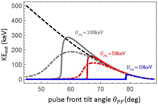
Figure 5. Single particle calculations of output electron kinetic energy KE_out resulting from acceleration from a finite Gaussian beam with radius 15 μm. The pulse duration is either 20fs (solid) or 50fs (dash-dot). The black dashed curve shows the non-relativistic prediction.

A second effect concerns the local shape of the pulse front. Although KE_out is determined by θ_PF and is not sensitive to the peak intensity, the transverse intensity dependence and the temporal pulse shape both affect the local curvature of the pulse front. Larger tilt angles lead to a longer flat section; shaping the transverse profile of the beam to a super-Gaussian also dramatically narrows the energy and angular distribution. A super-Gaussian shape is closer to the ideal tilted pulse that we used in our one-dimensional analysis.

These effects are illustrated by extending the single-particle analysis to finite beams with Gaussian and super-Gaussian transverse profiles (see Figure 6). Figure 6A shows how KE_out and the output angle θ_out depend on the starting X₀ position in the beam. The Gaussian beam profile shows much more variation than the super-Gaussian. The latter profile, which more closely approximates the ideal case described above, shows less curvature in the pulse front. In fact, the region in the −5 < X₀ < 0μm range shows just a 1% variation in output energy and less than 0.3% variation in output angle. Further improvement can be obtained by using larger spot size.

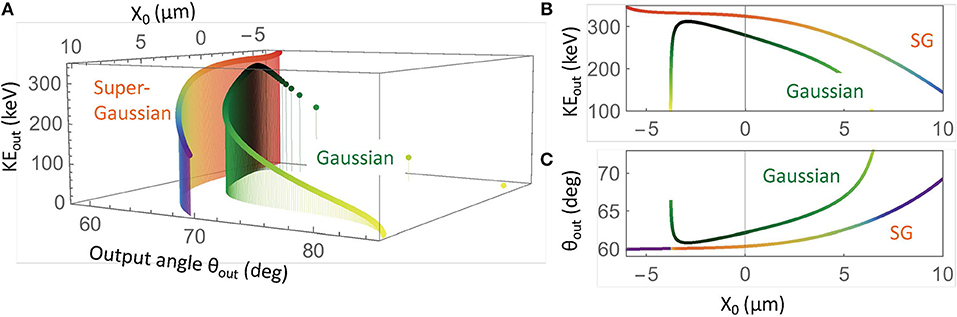
Figure 6. Single particle calculations for electron acceleration from a finite beam with radius 15 μm, a pulse duration of 20fs, a 60° PFT angle, and 100 keV peak ponderomotive potential. The two curves correspond to Gaussian and super-Gaussian transverse beam profiles. (A) output kinetic energy and angle as a function of the starting transverse position X₀. The color shading corresponds to the output energy. (B) Projection onto the KE_out − X₀ plane. (C) Projection onto the θ_out − X₀ plane.

Finally we consider the effect of the transverse intensity profile in the vertical (Y) direction. As seen above, the force is directed toward the local gradient of the spatio-temporal intensity profile. Figure 7 shows how KE_out and the output angle vary with the initial X₀, Y₀ position in the Z = 0 plane. Figures 7A–D show the results for the Gaussian and super-Gaussian beam profiles, respectively. The output angles are calculated as the cone angle deviation from the direction of the force, which is nominally at 60° to the Z−axis in the X−Z plane. For the Gaussian case, the angular dispersion is greater along the vertical direction than in the horizontal, since the tilted pulse front presents a wider face to the electrons. The super-Gaussian case illustrates, as we have seen above, how the energy and angular dispersion can be dramatically improved by engineering the pulse front intensity. The correlation of the output energy and angle with the starting electron position offers the possibility of externally filtering with an aperture to achieve better angular and energy dispersion (at the expense of beam current). For the Gaussian case, the energy dispersion δKE_out/〈KE_out〉 within a 5° cone angle is approximately 11%, while decreasing the cone angle to 1° gives δKE_out/〈KE_out〉 = 7%. This selection, however, is not efficient: the fractions of electrons starting in the circle with appreciable output energy shown in Figure 7A are 2 and 0.2%, respectively. The super-Gaussian case is much more promising. For a cone angle of 2° there are 43% of accelerated electrons, and these have δKE_out/〈KE_out〉 = 3%. Decreasing the cone angle to 0.5° contains over 25% of the electrons and an energy dispersion of 1%.

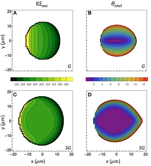
Figure 7. Single particle calculations of electron acceleration from a finite beam with radius 20 μm, a pulse duration of 20fs, a 60° PFT angle, and 200 keV peak ponderomotive potential. In the first row we calculate, as a function of the initial electron coordinate (X₀, Y₀, Z₀ = 0) and for a Gaussian (G) transverse beam intensity profile, the output (A) kinetic energy, KE_out and (B) the output angle, relative to the 60° direction of the force. The second row (C,D) shows the corresponding calculations for a super-Gaussian (SG) transverse beam profile. As indicated in the legends, the contour spacing for the energy plots is 20 keV and angle is 1 degree.

To obtain the intensity in the examples shown above would require a substantial pulse energy of approximately 450 mJ. We have chosen the ${\theta }_{PF}=60^{°}$ case since we can compare to the PIC simulations presented in the next section. However, increasing θ_PF dramatically decreases the pulse energy required for electron capture and acceleration. As an example, for ${\theta }_{PF}=85^{°}$, $U_p^{cap0}=1.8$ keV. For an intensity 2x over threshold, a spot radius of 10 μm and τ = 20fs, only 3.8 mJ of pulse energy is required. As the desired KE_out increases, so does the required input energy, but with proper shaping of the beam profile, a line focus (longer in the tilted direction) can be used to reach high intensity while obtaining good energy and angular distributions.

While at this stage we have not included the space charge effect on the electron dynamics, we can estimate the energy required to remove charge from a sphere. To remove 10 pC of charge from a sphere of radius 10 μm requires 67 nJ. While this energy is insignificant relative to the laser pulse energy, the energy required to remove the last electron is approximately 13.4 keV. The amount the energy dispersion is increased by the space charge will decrease as the accelerated kinetic energy increases. If the electron bunch is obtained from elsewhere, e.g., from photocathode emission, this space charge limitation can be circumvented.

4.3. Particle-In-Cell Simulations of Ponderomotive Tilted Pulse Acceleration

To explore this acceleration mechanism in more detail, we have begun to utilize the OSIRIS 4.0 particle-in-cell code [14, 15]. For the simulations presented here, we use the 2D, fully-relativistic, full field (non-cycle-averaged E and B fields) version of the code without any ponderomotive approximation. The tilted pulse is initialized at the focus at t = 0 as a fully compressed pulse in the space-time domain with a polarization perpendicular to the tilt direction. At present we restrict the use of the tilted pulse option to moderate tilt angle (≤ 60°) where the beam propagation has been tested against our propagation models [19]. The calculated capture potential for this angle corresponds to an intensity that is nearly relativistic (a₀ ≥ 0.7), where a₀ is the normalized vector potential, defined as $a_0=\sqrt{4U_{P0}/m_e{c}^2}$.

Figure 1 illustrates the acceleration of a square cold electron bunch 2.5 μm wide, initially at rest, by a pulse with ${\theta }_{PF}=60^{°}$, and an initial intensity that is well above threshold (a₀ = 1.25, U_P0 = 200 keV). The simulation parameters correspond to a pulse that is identical to that described in the previous section. The bunch is placed Z₀ = 20μm from the focal plane and is constructed such that the initial density (n_e) is far below the critical density ($n_e\ll 10^{-3}{n}_c$) in order to more closely model a distribution of non-interacting single particles. The plots are in the lab frame: the tilted pulse moves forward (to the right) at the speed of light. Note that the pulse duration increases with time owing to the geometrically induced chirp [19]. The electron bunch starts at rest, and is accelerated in a direction (61.1°) close to ${\theta }_{PF}=60^{°}$.

For the same conditions, Figure 8 shows the output p_x − p_z momentum distribution for the electron bunch. In blue, we see the distribution of the output electron momenta as calculated by OSIRIS. Overlaid in red and orange dots is the prediction of the single particle model for a 2.5μm wide distribution of initial transverse positions placed at Z₀ = 20μm and Z₀ = 0μm, respectively. The single particle model used for these simulations is fully-relativistic and ponderomotive and includes the pulse evolution effects described by Durfee et al. [19], which were neglected in previous sections as they are beyond the scope of this paper. There is strong agreement in the momenta distributions between the single particle model and the OSIRIS simulation for the 20 μm initial displacement. The 0 μm results are shown to illustrate how the momentum distribution changes with initial axial position.

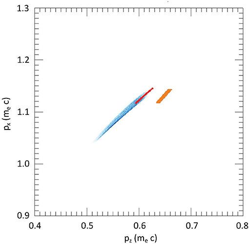
Figure 8. Calculations from the OSIRIS 4.0 PIC code for a 20 fs pulse duration, ${\theta }_{PF}=60^{°}$, and U_P0 = 200 keV, showing the distribution of output electrons (blue) in the p_z − p_x plane, starting from an electron bunch 2.5 μm wide in the X and Z directions centered at (X₀, Z₀) = (0, 20μm). The additional dots show the prediction from the single particle model for the same range of transverse initial positions, centered at (0, 0) (orange) and 0,20 (μm) (red).

There are a number of reasons for the small differences between the predictions of the relativistic single particle calculation and those of the OSIRIS simulation. The first is due to the fact that there are many particles in the OSIRIS simulation and space charge effects, while negligible for the densities considered here, will broaden the energy and angular spectra of the bunch. This effect has been seen in many other acceleration schemes. Additionally, OSIRIS uses an approximation of the laser pulse similar to Equation (12). The single particle model of the pulse used in this comparison includes more effects of the pulse evolution such as the evolution of the pulse front tilt angle and pulse duration though focus. These two effects, individually and in combination, change the dynamics of the acceleration process and could potentially lead to higher energies than predicted by OSIRIS. As stated before, we will further explore these effects, and how to potentially exploit them in future work.

Our objective in the calculation of Figure 8 was to compare our single-particle ponderomotive theory with a full field simulation. We see that the ponderomotive calculations are quite close to the full field results, with the latter resulting in somewhat larger energy spread. In future work, we plan to continue to use OSIRIS to explore the more interesting laser-plasma dynamics that occur in a real acceleration experiment. For example, rather than starting with a localized, stationary electron bunch, the electrons can be created through tunneling ionization of atoms in the early part of the pulse. Of particular interest is exploring the region where the ponderomotive approximation begins to break down and full-field effects become significant in the particle dynamics. As shown in Figure 5, the acceleration process benefits from using shorter duration pulses and predicting exactly how electrons will be accelerated using few-cycle pulses requires a better understanding of this transition region. We will investigate how more exotically shaped SSTF pulses, such as the super-Gaussian described in section 4.2, can optimize the energy-momentum landscape of the accelerated electrons. In future work, we will also investigate the dynamics of these pulses with higher electron densities, to better understand what brightnesses and emittances can be achieved with this scheme, as well as the wakefield regime.

5. Discussion and Conclusion

In this work, we have proposed an efficient laboratory-scale method of accelerating electrons from rest to relativistic energies using tilted ultrafast laser pulses. The tilt of the pulse front extends the interaction of the short pulse with the electrons such that the process acts at multiple time and length scales and thus requires a less energetic pulse for ponderomotive capture. At a given time within the pulse, an electron interacts with a beam with a width that is reduced by the pulse front tilt; this leads to larger ponderomotive force since the intensity gradient is larger. At the same time, the electron can interact with the full width of the beam as it accelerates. Correspondingly, the local pulse duration is transform limited, but the tilt of the pulse allows for an extended total duration of the pulse. This is in contrast to a non-tilted ponderomotive schemes where a captured electron does not have an extended period of time to interact with the pulse.

We have described this acceleration process with a simple ponderomotive model in one- and three-dimensions. We also demonstrated that this effect can be seen in more rigorous relativistic and full field simulations. Our analysis and simulations show that when the beam is engineered to a flat transverse profile, the method has promise to produce narrow energy and angular distributions for the accelerated electrons. Since the energy threshold can be modest with large tilt angle and short pulses, tilted pulse ponderomotive acceleration can be achieved with table-top laser systems, leading to possible applications in ultrafast electron diffraction. Our calculations indicate that the scheme can be staged to accelerate at least up to the 10MeV level (see Figure 4). In ongoing work we are considering other pulse structures that could go to higher energy for seeding laser wakefield electron accelerators.

Author Contributions

CD conceived and derived the original non-relativistic theory and began the original manuscript draft. AW ran the particle-in-cell simulations and contributed to the manuscript. Single particle calculations were performed and verified independently by both authors.

Funding

We gratefully acknowledge funding through the NSF/DOE Partnership for Basic Plasma Science and Engineering under NSF grant PHY-1619518.

Conflict of Interest Statement

The authors declare that the research was conducted in the absence of any commercial or financial relationships that could be construed as a potential conflict of interest.

Acknowledgments

The authors would like to acknowledge the OSIRIS Consortium, consisting of UCLA and IST (Lisbon, Portugal) for providing access to the OSIRIS 4.0 framework. Work supported by NSF ACI-1339893.

References

1. Richman BA, Bisson SE, Trebino R, Sidick E, Jacobson A. All-prism achromatic phase matching for tunable second-harmonic generation. Appl Opt. (1999) 38:3316–23. doi: 10.1364/AO.38.003316
2. Shirakawa A, Sakane I, Kobayashi T. Pulse-front-matched optical parametric amplification for sub-10-fs pulse generation tunable in the visible and near infrared. Opt Lett. (1998) 23:1292. doi: 10.1364/OL.23.001292
3. Hebling J, Yeh KL, Nelson K, Hoffmann M. High-power THz generation, THz nonlinear optics, and THz nonlinear spectroscopy. IEEE J Select Top Quant Electron. (2008) 14:345–53. doi: 10.1109/JSTQE.2007.914602
4. Zimmer D, Ros D, Guilbaud O, Habib J, Kazamias S, Zielbauer B, et al. Short-wavelength soft-x-ray laser pumped in double-pulse single-beam non-normal incidence. Phys Rev A. (2010) 82:013803. doi: 10.1103/PhysRevA.82.013803
5. Kazansky PG, Yang W, Bricchi E, Bovatsek J, Arai A, Shimotsuma Y, et al. “Quill” writing with ultrashort light pulses in transparent materials. Appl Phys Lett. (2007) 90:151120. doi: 10.1063/1.2722240
6. Vitek DN, Block E, Bellouard Y, Adams DE, Backus S, Kleinfeld D, et al. Spatio-temporally focused femtosecond laser pulses for nonreciprocal writing in optically transparent materials. Opt Express. (2010) 18:24673–8. doi: 10.1364/OE.18.024673
7. Zhu G, van Howe J, Durst M, Zipfel W, Xu C. Simultaneous spatial and temporal focusing of femtosecond pulses. Opt Express. (2005) 13:2153–9. doi: 10.1364/OPEX.13.002153
8. Durst ME, Zhu G, Xu C. Simultaneous spatial and temporal focusing for axial scanning. Opt Express. (2006) 14:12243–54. doi: 10.1364/OE.14.012243
9. He F, Xu H, Cheng Y, Ni J, Xiong H, Xu Z, et al. Fabrication of microfluidic channels with a circular cross section using spatiotemporally focused femtosecond laser pulses. Opt Lett. (2010) 35:1106–8. doi: 10.1364/OL.35.001106
10. Vitek DN, Adams DE, Johnson A, Tsai PS, Backus S, Durfee CG, et al. Temporally focused femtosecond laser pulses for low numerical aperture micromachining through optically transparent materials. Opt Express. (2010) 18:18086–94. doi: 10.1364/OE.18.018086
11. Block E, Greco M, Vitek D, Masihzadeh O, Ammar DA, Kahook MY, et al. Simultaneous spatial and temporal focusing for tissue ablation. Biomed Opt Express. (2013) 4:831. doi: 10.1364/BOE.4.000831
12. Tajima T, Dawson JM. Laser electron accelerator. Phys Rev Lett. (1979) 43:267–70. doi: 10.1103/PhysRevLett.43.267
13. Zewail AH. 4D ultrafast electron diffraction, crystallography, and microscopy. Annu Rev Phys Chem. (2006) 57:65–103. doi: 10.1146/annurev.physchem.57.032905.104748
14. Fonseca RA, Silva LO, Tsung FS, Decyk VK, Lu W, Ren C, et al. OSIRIS: a three-dimensional, fully relativistic particle in cell code for modeling plasma based accelerators. In: Computational Science — ICCS 2002. Berlin; Heidelberg: Springer (2002). p. 342–51.
15. Hemker RG. Particle-in-cell modeling of plasma-based accelerators in two and three dimensions. arXivorg. (2015).
16. Vicente H, Quéré F. Attosecond lighthouses: how to use spatiotemporally coupled light fields to generate isolated attosecond pulses. Phys Rev Lett. (2012) 108:113904. doi: 10.1103/PhysRevLett.108.113904
17. Oron D, Tal E, Silberberg Y. Scanningless depth-resolved microscopy. Opt Express. (2005) 13:1468–76. doi: 10.1364/OPEX.13.001468
18. Durfee CG, Squier JA. Breakthroughs in photonics 2014: spatiotemporal focusing: advances and applications. Photon J IEEE. (2015) 7:1–6. doi: 10.1109/JPHOT.2015.2412454
19. Durfee CG, Greco M, Block E, Vitek D, Squier JA. Intuitive analysis of space-time focusing with double-ABCD calculation. Opt Express. (2012) 20:14244. doi: 10.1364/OE.20.014244
20. Cerullo G, Nisoli M, De Silvestri S. Generation of 11 fs pulses tunable across the visible by optical parametric amplification. Appl Phys Lett. (1997) 71:3616. doi: 10.1063/1.120458
21. Block E, Thomas J, Durfee C, Squier J. Integrated single grating compressor for variable pulse front tilt in simultaneously spatially and temporally focused systems. Opt Lett. (2014) 39:6915–8. doi: 10.1364/OL.39.006915
22. Motz H, Watson CJH. The Radio-Frequency Confinement and Acceleration of Plasmas. Amsterdam: Elsevier (1967).
23. Akama H, Nambu M. A new theory of ponderomotive forces on a Vlasov plasma. Physica A. (1982) 116:155–62. doi: 10.1016/0378-4371(82)90235-7
24. Kentwell GW, Jones DA. The time-dependent ponderomotive force. Phys Rep. (1987) 145:319–403. doi: 10.1016/0370-1573(87)90063-9
Keywords: laser electron accelerators, ponderomotive force, ultrafast lasers, spatio-temporal pulse shaping, relativistic kinematics
Citation: Wilhelm AM and Durfee CG (2019) Tilted Snowplow Ponderomotive Electron Acceleration With Spatio-Temporally Shaped Ultrafast Laser Pulses. Front. Phys. 7:66. doi: 10.3389/fphy.2019.00066
Received: 14 November 2018; Accepted: 16 April 2019;
Published: 08 May 2019.
Edited by:
Jerome Faure, UMR7639 Laboratoire d'Optique Appliquée (LOA), FranceReviewed by:
Ilia L. Rasskazov, University of Rochester, United StatesXavier Davoine, CEA DAM Íle-de-France, France
Copyright © 2019 Wilhelm and Durfee. This is an open-access article distributed under the terms of the Creative Commons Attribution License (CC BY). The use, distribution or reproduction in other forums is permitted, provided the original author(s) and the copyright owner(s) are credited and that the original publication in this journal is cited, in accordance with accepted academic practice. No use, distribution or reproduction is permitted which does not comply with these terms.
*Correspondence: Charles G. Durfee, cdurfee@mines.edu