Disrupted modularity and local connectivity of brain functional networks in childhood-onset schizophrenia
- 1 Department of Psychiatry, Behavioural and Clinical Neuroscience Institute, University of Cambridge, Cambridge, UK
- 2 Child Psychiatry Branch, National Institute of Mental Health, Bethesda, MD, USA
- 3 David Geffen School of Medicine at University of California, Los Angeles, CA, USA
- 4 Department of Psychiatry, University of Wisconsin School of Medicine and Public Health, Madison, WI, USA
- 5 Prince of Wales Medical Research Institute, University of New South Wales, Sydney, NSW, Australia
- 6 GlaxoSmithKline Clinical Unit Cambridge, Addenbrooke’s Hospital, Cambridge, UK
Modularity is a fundamental concept in systems neuroscience, referring to the formation of local cliques or modules of densely intra-connected nodes that are sparsely inter-connected with nodes in other modules. Topological modularity of brain functional networks can quantify theoretically anticipated abnormality of brain network community structure – so-called dysmodularity – in developmental disorders such as childhood-onset schizophrenia (COS). We used graph theory to investigate topology of networks derived from resting-state fMRI data on 13 COS patients and 19 healthy volunteers. We measured functional connectivity between each pair of 100 regional nodes, focusing on wavelet correlation in the frequency interval 0.05–0.1 Hz, then applied global and local thresholding rules to construct graphs from each individual association matrix over the full range of possible connection densities. We show how local thresholding based on the minimum spanning tree facilitates group comparisons of networks by forcing the connectedness of sparse graphs. Threshold-dependent graph theoretical results are compatible with the results of a k-means unsupervised learning algorithm and a multi-resolution (spin glass) approach to modularity, both of which also find community structure but do not require thresholding of the association matrix. In general modularity of brain functional networks was significantly reduced in COS, due to a relatively reduced density of intra-modular connections between neighboring regions. Other network measures of local organization such as clustering were also decreased, while complementary measures of global efficiency and robustness were increased, in the COS group. The group differences in complex network properties were mirrored by differences in simpler statistical properties of the data, such as the variability of the global time series and the internal homogeneity of the time series within anatomical regions of interest.
Introduction
One of the most ubiquitous properties of complex systems, like large-scale functional brain networks, is that they generally have a modular community structure (Bullmore and Sporns, 2009). Using resting-state fMRI analysis, functional communities or modules can be broadly defined as groups of brain regions whose fMRI time series are similar to each other and dissimilar from other groups. How to partition the brain into such functional communities, and the related question of how to assess the quality of these partitions, are methodological issues that have been approached from the perspectives of both unsupervised learning and graph theory. In the context of unsupervised learning, where brain regions are considered as objects in n-dimensional functional space to be classified into their “natural” groups, hierarchical cluster analysis has been used to decompose the brain into a small number of functional modules that resemble known patterns of neural connectivity (Cordes et al., 2002; Salvador et al., 2005). In graph theory, on the other hand, brain regions are nodes (or vertices), functional connections between nodes are edges (or links), and modules are groups of nodes with many intra-modular links to each other but few inter-modular links to external groups (Newman and Girvan, 2004). Graph theoretical work has shown that human brain functional modules are hierarchically organized (Meunier et al., 2009b; Bassett et al., 2010), that their structure is altered in normal aging (Meunier et al., 2009a) and in adolescence (Fair et al., 2009), and that their structure is relatively consistent for fMRI and diffusion spectrum imaging (DSI) of the same subjects (Hagmann et al., 2008). The brain, at least the healthy brain, is a modular system.
Here we test the hypothesis that the normal modular community structure of functional brain networks might be somehow disrupted in neuropsychiatric disease, specifically in schizophrenia. There are theoretical reasons to posit that the brain’s modularity is crucial in terms of its evolution and healthy neurodevelopment. Modularity may allow the brain to adapt to multiple, distinct selection criteria over time (Kashtan and Alon, 2005). Modules may also represent stable subcomponents of the brain, which facilitate the construction of a complex system from simple building blocks (Simon, 1962). In the context of the recent focus on the developmental phenotypes of neuropsychiatric disease (e.g., Gogtay et al., 2008; Giedd et al., 2009), it makes sense to measure properties of neuroimaging data, such as modularity, that are theoretically linked to network development and that may provide sensitive markers of abnormal brain development in disorders such as schizophrenia. In fact, dysmodularity in schizophrenia has already been proposed as a neuropsychological theory, implying the breakdown of information encapsulation between brain systems that are specialized to carry out different tasks (Fodor, 1983; David, 1994). In the functional neuroanatomical context, possible examples might include pathological crosstalk between inner speech and auditory areas in the pathogenesis of hallucinations (Shapleske et al., 2002), or between left and right prefrontal cortex in working memory tasks (Lee et al., 2008). However, it is clear that this point can be argued from both sides: For example, patients seem to be more susceptible than controls to the Müller-Lyer illusion (Pessoa et al., 2008), a visual illusion that persists in spite of explicit knowledge about the nature of the illusion, which has been held up as an exemplar of perceptual modularity. At any rate, it is not obvious how to relate the notions of psychological modularity and topological modularity as it is quantified in complex systems, and the dysmodularity hypothesis has not yet been tested with any rigor in neuroimaging experiments.
There are methodological barriers to testing this hypothesis. As already noted there are a number of possible ways in which the community structure of functional networks can be described, and these alternatives have not been comparatively evaluated. Moreover it is non-trivial to make comparisons of modularity, however measured, between two groups of brain graphs with different topological properties. Even random graphs show complex properties including modularity to an extent that varies depending on the number of nodes and edges in the graphs (Bollobás, 1985; Anderson et al., 1999; Guimerà et al., 2004). Network properties can change dramatically around the percolation threshold where graphs become node-connected (Dorogovtsev et al., 2008), where “node-connected” means that none of the nodes is entirely isolated, each is linked by at least one edge to a single giant connected cluster. To ensure that statistical comparisons of brain network properties are meaningful, therefore, all of the graphs should ideally have the same number of nodes and edges, and they should all be node-connected. This last point is crucial because graphs constructed by global thresholding from data on different subjects may often show different degrees of node-connectedness, especially if the graphs are sparse. While differences in node-connectedness, e.g., as measured by percolation threshold, may be informative in their own right (Chen et al., 2007), they should ideally be controlled when considering group differences in other more edge-based network metrics such as degree. One conceptually simple way of doing this is to restrict evaluation of network metrics to a range of connection densities for which all graphs are node-connected (Bassett et al., 2008; Lynall et al., 2010). However, this approach may preclude comparative analysis of network properties at sparser connection densities where complex topological features such as modularity are typically most prominent.
We explore some of these methodological issues in the context of a preliminary investigation of the modularity and other properties of brain functional networks measured using fMRI in childhood-onset schizophrenia. We devise a way of applying a local threshold to construct brain graphs, which ensures that all of the graphs are node-connected at minimal densities, in contrast to the variability of node-connectedness that typically arises when graphs are constructed by a global threshold. We compare standard graph theoretical modularity results with the results of an unsupervised learning approach, using a generalization of the k-means algorithm known as partition around medoids (PAM), and a multi-resolution spin glass algorithm. In addition to modularity, we estimate several other properties of the graphs, most of which have previously been investigated in adult-onset schizophrenia (Liu et al., 2008; Rubinov et al., 2009; Lynall et al., 2010). Finally, we ground the complex network analysis by looking at simpler properties of the fMRI time series in these subjects, such as the variability of the time series and its internal homogeneity within anatomical regions of interest. We find evidence in support of network dysmodularity in COS, and explain this finding in the context of the other properties of the fMRI phenotype that we investigate. To our knowledge this is the first study to report less modular brain organization or abnormal community structure of brain functional networks in any human population.
Materials and Methods
Sample
Thirteen COS patients and 19 controls or “normal volunteers” (NV) were recruited as part of an ongoing National Institute of Mental Health study of COS and normal brain development (ClinicalTrials.gov Identifier: NCT00001246). All patients met the DSM-IV criteria for childhood-onset schizophrenia, and consent was acquired from both patients and their legal guardians. The populations did not differ significantly in terms of age (COS sample mean age = 18, standard deviation = 4; NV sample mean age = 19, standard deviation 4; t-test p-value = 0.29) or gender (8 female, 5 male COS; 10 female, 9 male, NV; chi squared test p-value = 0.89).
Image Acquisition and Preprocessing
All images were acquired using a 1.5T General Electric Signa MRI scanner located at the National Institutes of Health Clinical Center (Bethesda, MD). One anatomical T1-weighted fast spoiled gradient echo MRI volume was acquired: TE 5 ms; TR 24 ms; flip angle 45°; matrix 256 × 256 × 124; FOV 24 cm. In addition, two sequential 3 min EPI scans were acquired while subjects were lying quietly in the scanner with eyes closed: TR 2.3 s; TE 40 ms; voxel 3.75 mm × 3.75 mm × 5 mm; matrix size 64 × 64; FOV 240 mm × 240 mm; 27 interleaved slices. The first four volumes of each functional scan were discarded to allow for T1 equilibration effects. AFNI was used for slice time correction and for motion correction (Cox, 1996). In terms of motion, the maximum displacement of brain voxels due to motion did not differ significantly between the groups (sample mean COS maximum displacement = 2.45 mm; sample mean NV maximum displacement = 1.93 mm; t-test p-value = 0.41). FSL’s FLIRT (Jenkinson and Smith, 2001; Jenkinson et al., 2002) was used to register each subject’s functional scans to that subject’s structural scan using a 6 degrees of freedom transformation, and to register the structural scan to MNI stereotactic standard space using a 12 degrees of freedom transformation. Although registering both pediatric and adult brains to the MNI adult brain template image could result in some age-specific differences in spatial normalization, these differences are unlikely to affect fMRI results because of fMRI’s relatively low spatial resolution (Burgund et al., 2002; Kang et al., 2003) and because functional activity is represented by regional mean time series averaged over multiple voxels comprising regions of the parcellation template image. Both these factors suggest that the scale of any possible age-related mis-registration is likely to be small in comparison to the relatively coarse-grained scale of functional network analysis applied to the data. We note that adult template images have previously been used as a basis for normalization of fMRI data on participants in similar and even younger age-ranges than our sample (Durston et al., 2003; Turkeltaub et al., 2003; Cantlon et al., 2006; Crone et al., 2006; Galvan et al., 2006).
Wavelet Measures of Variability and Covariability at Different Scales
For each functional scan, 111 anatomical regions were defined using the combined cortical and subcortical Harvard-Oxford Probabilistic Atlas (Smith et al., 2004) thresholded at 25%. Because of low quality signal due to susceptibility artifacts in some regions, quantified as the majority of a region being absent from the EPIs of the majority of subjects, the brainstem and 5 bilateral cortical regions at the inferior frontotemporal junction were excluded, which resulted in a dataset of 100 regions for each functional scan. In addition to the voxel time series, 100 regional time series were estimated by averaging the voxels within each of the regions, while one global time series was estimated by averaging the voxels within all of the regions.
The maximal overlap discrete wavelet transform (MODWT) with a Daubechies 4 wavelet was used to band-pass filter the time series (Percival and Walden, 2006) and, in what follows, we will focus on the results obtained using the scale 2 frequency interval, 0.05–0.111 Hz. This frequency scale was chosen to minimize the impact of higher frequency physiological noise while maximizing the degrees of freedom available for wavelet correlation, as well as for consistency with previous work. Wavelet coefficients with boundary effects from the MODWT were excluded, and the coefficients of the sequential functional scans were concatenated to form a single series of 144 wavelet coefficients which was the basis for all further analyses of variability and covariability (e.g., see Figures 2B,D).
Variability of the global and regional signals
We quantified the variability of the low frequency MRI signal simply as the sample variance of the MODWT wavelet coefficients at scale 2. (To make comparisons between the variability of the signal at different temporal scales, the wavelet variances would have to be corrected for the redundancy of the MODWT, but we focus exclusively on differences between the clinical populations at the same scale.) Variability was estimated for each of the anatomical regions and also for the global signal.
Covariability between and within regions
The wavelet correlation, −1 ≤ ri,j ≤ +1, was used as an estimate of the covariability between two time series i and j. For N anatomically defined regions, this value was found for all (N2 − N)/2 pairs of regions. The regional strength of connectivity s(i) for a region i was defined as the mean of the correlations with the N − 1 other regions:
We also explored the covariability of the voxels within each anatomical region, treating each anatomical region as a distinct subnetwork. If x is a voxel within a region i, and K is the number of voxels within i, the average voxel connectivity strength s(x) over all K is a measure of the internal homogeneity of the signal from region i. Although at a different spatial and temporal scale, this statistic is similar to so-called regional homogeneity (ReHo; Zang et al., 2004), which has been calculated between neighboring voxels. For greater consistency with this prior work, we also calculated Kendall’s coefficient of concordance, 0 ≤ W(i) ≤ +1, between the voxels in each region i:
Here, K is the number of voxels in region i; n is the length of the time series; Rx is the sum of the ranks of the xth voxel; and  is the mean of Rx, over all K voxels. The numerator in Eq. 2 is the variance of the sums of the ranks, and the denominator is the maximum possible variance given the number of voxels and the length of the time series (Sheskin, 2007). The advantages of this statistic are that it is non-parametric and that it is defined for a region containing any number of voxels. The average regional concordance is the mean of W over all N regions.
Graph Construction
Note that R code used for graph construction is publicly available at http://brainnetworks.sourceforge.net, and the Appendix contains definitions of some commonly used graph theoretical terms. To make a graphical model of brain network connectivity, the usual approach is to generate a binary adjacency matrix A from a continuous association or connectivity matrix C. It is also possible to measure network properties by analysis of the connectivity matrix using tools which do not require a binary thresholding operation to generate an adjacency matrix. Here we explored two different (global and local) thresholding methods to construct an adjacency matrix from the 100 × 100 connectivity matrix, C, where Ci,j = |ri,j|, the absolute wavelet correlation coefficient for a pair of regional time series i and j. We also investigated two complementary methods – the unsupervised learning algorithm “partition around medoids” (PAM) and the multi-resolution spin glass model of modularity – to measure network properties without thresholding the connectivity matrix.
Most human neuroimaging studies to date have used global thresholding to construct functional brain networks. Using this method, any |ri,j| of the functional connectivity matrix greater than a threshold, τ, implies an edge in the corresponding element of the adjacency matrix, A, meaning that Ai,j = 1. If ri,j < τ, then Ai,j = 0. Thresholding at a different value of τ creates a graph with a different edge density or cost, which is the number of edges in a graph comprising N nodes, divided by the maximum number of possible edges, (N2 − N)/2. A difficulty with global thresholding is that at sparse densities it can result in graphs that are not node-connected, i.e., there is not a finite path between every pair of nodes. Disconnectedness of the graphs affects the quantitative values of many network metrics. Therefore, comparisons of network metrics between different subjects may be biased if the network for one subject is connected at the chosen threshold, but the network for the other subject is fragmented or disconnected. We anticipated that this might be a significant challenge in making a fair comparison between networks estimated in healthy volunteers versus patients with COS.
To address the issue of disconnectedness that can arise as a result of global thresholding, we explored an alternative thresholding method that forces graphs to be connected even at sparse densities. To this end we made use of the standard graph theoretical concepts of the minimum spanning tree (MST; Kruskal, 1956; Prim, 1957) and the k nearest neighbor graph (k-NNG; Eppstein et al., 1992). The k-NNG is composed of those edges that link each node to the k nearest other nodes, where “nearest” in this case means highest functional connectivity. The MST is composed of those edges that node-connect the graph with the lowest possible number of edges and the highest possible functional connectivity. Put differently, an MST of a graph is a node-connected subgraph that includes the minimum total weight, and here we interpret the weight of an edge between two nodes as one minus the nodes’ functional connectivity. Although in theory there could be more than one MST or k-NNG for a given network, in practice this does not occur in our data. Algorithmically, the MST can be found by starting with the 1-NNG, that is by including an edge between every node and its single nearest neighbor. If the 1-NNG is connected, then it is identical to the MST; if the 1-NNG is disconnected, including fragmented groups of nodes with no finite path between them, then additional edges are added to link these fragments. For a given graph with N nodes, the MST always has N − 1 edges, which include the edges of the 1-NNG as a subset.
Although the MST itself can be used as a sparse representation of the whole network, it is somewhat implausible biologically because the MST is by definition acyclic (no loops or triangles) and its edges do not form clusters or cliques. For example, the clustering coefficient (Watts and Strogatz, 1998) of an MST will always be zero. For this reason, it has been previously proposed to start with the MST as a minimal connected skeleton of the brain network and then grow the tree by adding extra edges according to a standard global thresholding rule (Hagmann et al., 2008). Alternatively, we developed a new method to grow the MST by adding extra edges according to a local thresholding rule. Specifically, we add the edges of the k-NNG in step-wise fashion, for higher and higher k. Since the MST is a connected superset of the 1-NNG, we generalize the concept to connected supersets of the k-NNG. See Figure 1 for an illustration of these different graph construction methods, applied to a “toy” connectivity matrix composed of 11 of the 100 nodes of a typical subject.
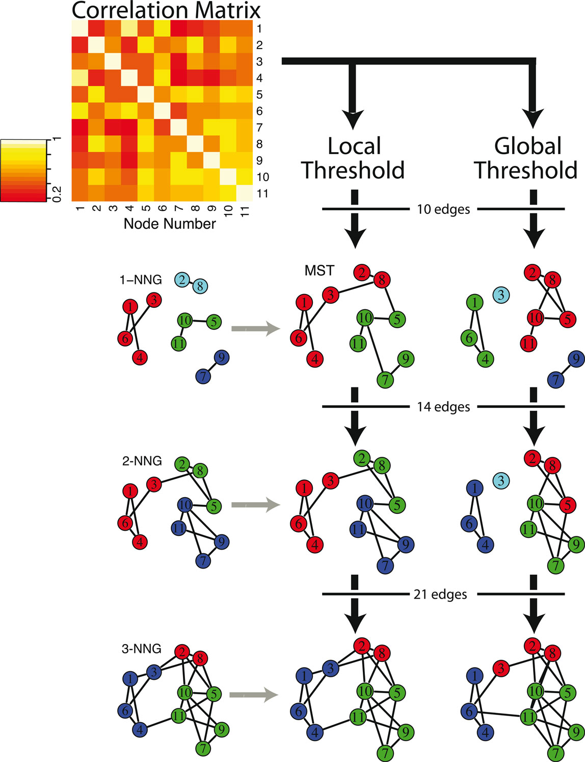
Figure 1. Schematic illustrating local and global thresholding methods, and how these methods impact on the modular structure of graphs constructed from a correlation matrix. Starting with a model correlation matrix, which shows the functional connectivity between a subset of 11 brain regions for one subject, the two different thresholding methods are used to construct graphs with increasing numbers of edges. On the left, applying a local threshold produces connected supersets of the k nearest neighbor graph (k-NGG), which includes edges for each node’s k highest functional connections, shown here for k = 1, 2, 3. The minimum spanning tree (MST) is a connected superset of the 1-NNG, and connects all 11 nodes with the lowest possible number of edges and the highest possible functional connectivity. On the right, applying a global threshold simply includes edges between the pairs of nodes with the highest functional connectivity in order. Nodes of the same color are in the same module, as determined by the fast greedy algorithm, showing the influence of graph construction and edge density on the modular partition.
A final alternative is to avoid thresholding altogether, using network measures that can be appropriately applied to the unthresholded connectivity matrix. This sidesteps the potentially arbitrary decision of how to threshold the connectivity matrix. However, the unthresholded graphs – also called “complete” graphs – will in general have lower signal-to-noise. In addition, there is less heterogeneity between the graphs of different subjects, as the adjacency matrices are identical and only the weights of the edges can differ. Finally, only some network measures, such as modularity (discussed below), have analogs that can be applied to weighted complete graphs.
Global Network Measures
We report network properties over the whole of range of edge density or cost, from 0.02 to 0.98 at 0.02 intervals, for both globally and locally thresholded graphs. As a summary statistic, we also calculated the mean of each metric over the range of costs from 0.3 to 0.5. This range was chosen for several reasons: (1) most of the globally thresholded graphs become connected by a cost of 0.3; (2) previous work suggests that above a cost of 0.5 graphs become more random (Humphries et al., 2006) and less small-world; and (3) the network measures are relatively constant over this range. Statistics were calculated in R (R Development Core Team, 2009) using original code as well as the following packages: wmtsa, brainwaver, cluster, MASS (Venables and Ripley, 2002), and igraph (Csardi and Nepusz, 2006).
Randomized graphs
It is important to contrast the brain graphs with comparable random graphs (Watts and Strogatz, 1998). We used two procedures to construct such graphs. With one method, the edges of the graph were replaced by edges chosen completely at random, with every pair of nodes having an equal probability of being connected in the new graph. Thus the only constraint is that the random graphs have the same number of nodes and edges as the original graphs (Erdös and Rényi, 1959). Alternatively, the graphs were “rewired” so as to preserve the degree distribution of the original graph. This is accomplished by picking two edges at random, between nodes A and B and between nodes C and D, and replacing these with edges between nodes A and C and between nodes B and D. Enough iterations of this process ensure a randomized graph where every node still has the same degree as in the original graph (Milo et al., 2004). We also explored graphs that were only partially randomized, where some proportion of the edges had undergone one or the other randomization procedure.
Global efficiency
The global efficiency, E(G), of a graph G is

where Li,j is the minimum path length, or the minimum number of edges that must be traversed between regions i and j (Latora and Marchiori, 2001; Achard and Bullmore, 2007). Note that if there is not a finite path between nodes i and j, then (1/Li,j) = 0. The regional or nodal efficiency of one brain region can also be calculated by averaging 1/Li,j over each node separately. When calculating Li,j for weighted graphs, the edges themselves are treated as varying in length according to the weight matrix W, where Wk,l = 1 − Ck,l. For weighted graphs, the global efficiency at a given cost is normalized by dividing by the global efficiency of the unthresholded, complete graph. (Theoretically, this is the case for binary global efficiency as well, but the global efficiency of the complete graph is 1).
Local efficiency
The local efficiency, Eloc(G, i), of a node i in a graph G is computed as:

Here, Gi is the subgraph including only the neighbors of i (not i itself), and E(Gi) is the global efficiency of Gi. The local efficiency of the graph is the average of the local efficiency of all of its nodes. This metric can be extended to weighted graphs in the same manner as global efficiency (Latora and Marchiori, 2001; Achard and Bullmore, 2007).
Clustering
The regional or nodal clustering coefficient, C(G, i), of a node i in a graph G is the ratio of connected triangles, δv to connected triples, τv. In other words, it is the proportion of i’s neighbors that are also neighbors of one another. For the graph as a whole, the clustering coefficient is:

where V′ is the set of nodes with degree >2 (Watts and Strogatz, 1998; Schank and Wagner, 2004). Clustering is a measure of the locally aggregated structure in a graph.
Small-worldness
Small-world networks have high clustering, C, but low average minimum path length, L, compared to random networks. The small-worldness, σ(G), of a graph G is calculated as:
Here, CR is the clustering of random graph rewired so as to preserve the degree distribution of G, and LR is the average minimum path length of such a random graph. For connected graphs, the average minimum path length is identical to the inverse of the (unweighted) global efficiency, so we can also write λ(G) = ER/E(G). For disconnected graphs, formally σ(G) is undefined, but we can again substitute λ(G) = ER/E(G) to get a related quantity. A network is generally accepted as “small-world” if σ > 1 (Humphries et al., 2006).
Robustness
As a measure of robustness, we looked at the resistance of the network to fragmentation after removal of nodes either in random order or in decreasing order of their degree. Suppose that there are M fragments in the network, i.e., M subgraphs that are connected internally but disconnected from each other. Resistance to fragmentation is defined as:
where Nj is the number of nodes in fragment j, and N is the number of nodes in the graph. N − 1 nodes are removed in order, and robustness is the mean of R over all of these smaller graphs (Chen et al., 2007).
Modularity
We explored modularity using three complementary methods from unsupervised learning and graph theory: partition around medoids (PAM), fast greedy optimization of thresholded graphs, and simulated annealing of a spin glass model. See Figure 1 for an illustration of these methods, applied to a model network.
PAM
PAM, like the more widely known method of hierarchical clustering, is an unsupervised learning algorithm that does not require thresholding of the connectivity matrix (Kaufman and Rousseeuw, 1987). Modules are referred to as “clusters” in the unsupervised learning literature, but to avoid confusion we will use the graph theory terminology. PAM is a generalization of the k-means algorithm that is more robust to noise and outliers. It requires as inputs the number of expected modules and the dissimilarity between every pair of nodes i and j. For our purposes, the dissimilarity between i and j is defined as 1 − Ci,j for the connectivity matrix C. The algorithm finds each module a representative node (medoid), and assigns other nodes to modules so as to minimize their dissimilarity with these medoids. The silhouette width, S, can be used to assess the quality of this partition:
Here, i is a brain region, Ai is the mean dissimilarity between i and the other regions in its module, and Bi is the mean dissimilarity between i and the regions in the next nearest module. The silhouette width ranges from −1 to 1, and a high positive number means that i is well-classified. The mean silhouette width over every region provides a global measure of the quality of the partition. It is explored over a range of possible numbers of modules.
Graph theoretical modularity
The modularity, Q, of a graph G can be quantified as the proportion of G’s edges that fall within modules, subtracted by the proportion that would be expected due to random chance alone, for a given partition of nodes into modules. This can be written as (Newman and Girvan, 2004):

Here, m is the total number of edges; Aij = 1 if an edge links i and j and 0 otherwise; δ(Mi, Mj) is 1 if i and j are in the same module and 0 otherwise, and ensures that only intra-modular edges are added to the sum; finally, Pij is the probability that there would be an edge between i and j, given a random graph comparable to G. The value of Pij depends on what counts as a “comparable” random graph, the so-called null model. We use

where ki is i’s degree, the number of other nodes to which i is linked by an edge. We include this information in the null model because it affects the expected proportion of intra-modular edges.
Weighted modularity is calculated analogously. In Eqs 9 and 10, the total number of edges, m, becomes the total weight of the edges. The degree, ki, is replaced by i’s strength, which is the total weight of i’s edges. And finally the adjacency matrix, A, is replaced by the weight matrix, W; the ones in the adjacency matrix are replaced weights of the edges. Pij can be understood as the expected weight between i and j. Note that an edge’s weight in the weighted modularity calculation is actually one minus that edge’s weight in the calculations of weighted global or local efficiency.
There are several known algorithms to assign nodes to modules so as to maximize Q. The principal benefits of the fast greedy algorithm that we use are its computational speed and the fact that it has been used in prior fMRI studies (e.g., Meunier et al., 2009a,b). This algorithm starts by assigning each node to its own module, and then agglomerates modules in a step-wise fashion, choosing the 2 modules whose combination results in the highest Q. The modularity value for the graph is then the highest Q that results throughout this step-wise process (Clauset et al., 2004). We applied this algorithm over the full cost range using a global threshold and a local threshold, for weighted and unweighted graphs.
Multi-resolution spin glass model
Finally, we employed a graph theoretical algorithm that looks at the modular structure at different resolutions. It has been shown that there is a resolution limit to modularity, in that modules smaller than a certain size are not found by traditional approaches (Fortunato and Barthélemy, 2007). Thus the modular structure is biased toward a certain scale, which is particularly problematic when considering a multi-scale system like the brain. This problem can be addressed by adding an additional parameter into the definition of modularity. One approach (Reichardt and Bornholdt, 2006) equates the problem of partitioning a graph with the problem of minimizing the energy of an infinite range Potts spin glass model, where the group indices become spin states. Groups of nodes with dense internal connections end up having parallel spins. The Hamiltonian, ℋ, of a graph G is:

Here, γ > 0 is the additional, adjustable parameter. The γ parameter can be thought of as a resolution parameter, such that higher values result in higher number of modules, each of which has fewer members on average. To find the optimal partition at different resolutions, this quality function ℋ is minimized for different values of γ, using a simulated annealing approach. When γ = 1, minimizing this function is equivalent to maximizing modularity as defined in Eq. 10. One of the virtues of the spin glass algorithm is that, although it can be applied to graphs with any cost, it can also be appropriately applied to the unthresholded connectivity matrix, so we do not have to set a threshold (Heimo et al., 2008). One drawback of the algorithm is that there is no obvious way to choose between the partitions found with different values of γ. A potential solution is to focus on partitions that are stable over a range of values of γ if a such a partition exists (Lambiotte, 2010). It is also informative to look at the pattern of how the modular structure changes with different values of γ.
Results
Variability and Covariability of the MRI Time Series
There were clear differences between groups in terms of some statistically elementary properties of the images: global mean variability, strength of functional connectivity, and within-regional homogeneity. The global mean wavelet-filtered time series had significantly reduced variability in COS versus healthy volunteers (sample mean global variability NV = 2.08; COS = 0.95; permutation test p = 0.007; Figures 2A,B). There was a similar but less obvious trend towards decreased variability at the regional level in the COS population (Figures 2C,D). The mean strength of between-regional functional connectivity was significantly reduced in COS versus healthy volunteers (sample mean pair-wise wavelet correlation NV = 0.37; COS = 0.26; permutation test p = 0.001). This finding extends to decreased strength of functional connectivity at the level of individual regions, if we consider each region’s average wavelet correlation with all other regions of the brain (Figure 2E). The within-regional homogeneity of the fMRI signal was significantly reduced in COS versus healthy volunteers (sample mean regional concordance, Kendell’s W, NV = 0.11; COS = 0.08; permutation test p = 0.002). This decreased regional concordance extends to almost every region considered individually (Figure 2F).
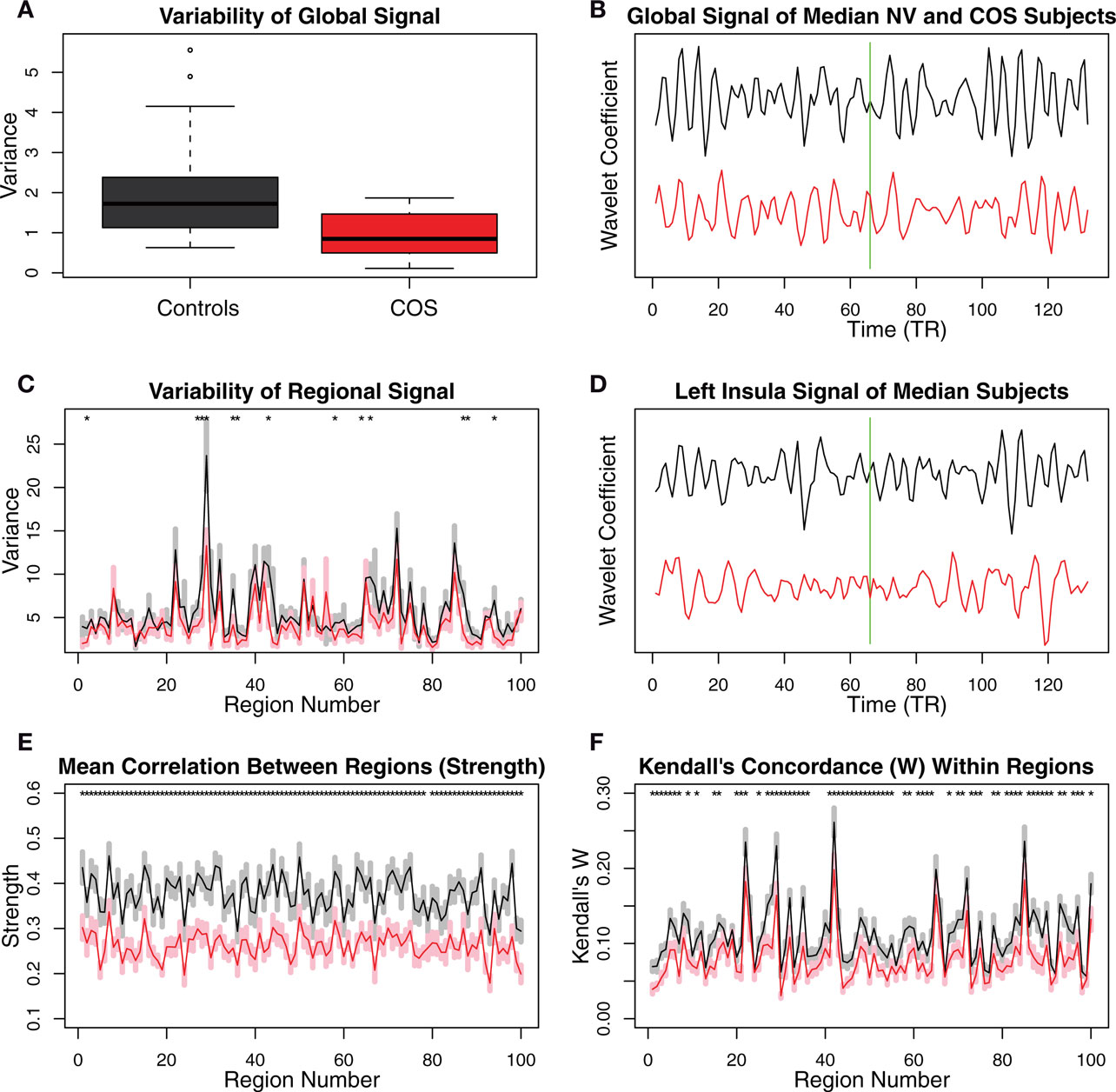
Figure 2. Plots showing differences between the schizophrenic patients and the controls in terms of relatively simple, non-graph-theoretical properties of their MRI time series. (A) The variability in the scale 2 (0.05–0.111 Hz) global MR signal is higher in the controls than in the COS population. (B) The difference in the variability of the global MR signal is illustrated with the time series from the median subjects of each population. The green line shows the boundary between the successive scans, whose wavelet coefficients were concatenated. (C) There is a trend toward greater variability in the MR signal of anatomical regions, in the control population relative to the COS population. (D) The difference in the variability of the regional MR signals is illustrated with the time series from the median subjects of each population for one of the regions that shows a difference, the left insula. (E) Regional strength, the average wavelet correlation between each region and every other region, is decreased in the COS population. (F) Kendall’s coefficient of concordance (W), a measure of the homogeneity of the signal within each anatomical region, is decreased in the COS population. Error bars are standard mean error, and asterisks signify p < 0.05 uncorrected p-value from a t-test.
Graph Theoretical Properties
Comparing locally thresholded with globally thresholded graphs, both methods of network construction revealed a similar pattern of results. However, there were clear advantages to using locally thresholded networks, because differences in node-connectedness complicate group comparisons on other metrics at low costs. On average, using a global threshold, not all of the graphs become connected until a cost of 0.3, and the healthy volunteers generally become connected at higher costs than the patients (for some healthy subjects the minimum cost of node-connectedness >0.5). Another way of saying this is that the percolation threshold is set higher in healthy volunteers than in people with COS. On one level this difference is perhaps diagnostically interesting, but it is also methodologically inconvenient because comparison of any other network parameter between the two groups will be confounded if more of the networks are connected in one group than the other. For this reason we judged it was preferable to use a local thresholding method to compare graphs with low connection density.
For both types of thresholding, we found that simple binary functional networks on average showed decreased clustering and local efficiency in people with COS, relative to the healthy controls. These measures of reduced local connectivity in COS were associated with increased global efficiency and robustness, both implying relatively stronger global connectivity in COS (Table 1; Figure 3). Broadly speaking, the balance of global and local connectivity in functional brain networks was abnormally shifted toward the global end of the scale in childhood-onset schizophrenia. This can be quantified by a change in the small-worldness parameter σ. Although networks in both groups were small-world (σ > 1) over the whole cost range, indicating that they generally had greater-than-random clustering but near-random global efficiency, small-worldness was abnormally reduced because of the disproportionate reductions in local connectivity or clustering in the COS group.
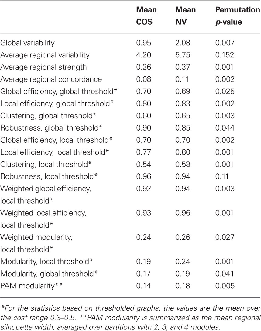
Table 1. For 18 metrics, the mean value for the childhood-onset schizophrenia (COS) population, the mean value for the controls or “normal volunteers” (NV), and the p-value for a permutation test of the group difference. Tests were based on 2000 permutations.
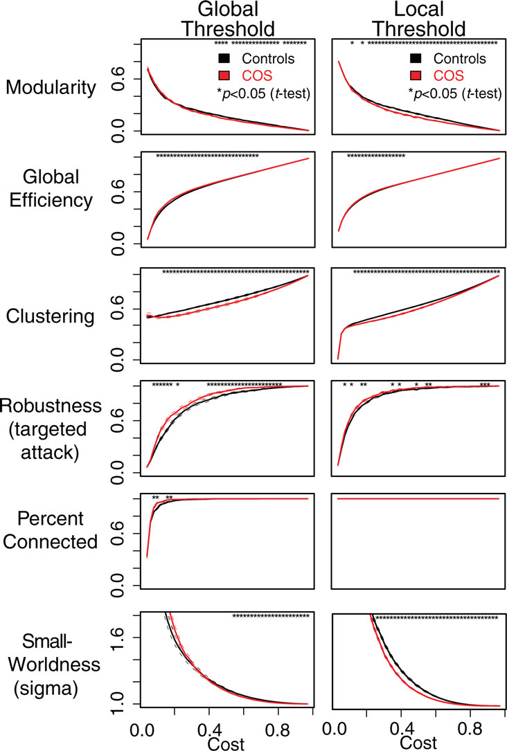
Figure 3. Plots showing differences between the schizophrenic patients (red) and the controls (black) in terms of the graph theoretical properties of the brain networks, which have been constructed using local and global thresholding methods. The two methods produce a similar pattern of group differences. However, local thresholding ensures connected graphs and appears to be more sensitive to group differences in some complex network metrics. The six different graph theoretical measures are shown as a function of connection density or topological cost, which is the proportion of edges included. Error bars are standard mean error, and asterisks signify an uncorrected p < 0.05 for a t-test between the COS population and control population.
The pattern of reduced local clustering and increased efficiency at a whole brain level was reflected by a convergent pattern of results at a regional level of analysis (Figure 5). Nineteen anatomical regions had significantly reduced clustering in COS relative to controls [permutation with 2000 tests, corrected for N = 100 multiple comparisons with false positive correction p < (1/N) = 0.01]. The cortical regions with abnormally reduced local connectivity included left and right superior temporal gyrus, left ventral occipital cortex, right cingulate, right insula, and right frontal operculum. In addition there were subcortical decreases of clustering bilaterally in the thalamus, caudate, and accumbens. The results for regional efficiency were less striking, but five anatomical regions had significantly increased efficiency in COS relative to the controls after correction for multiple comparisons. These increases were located in the right inferior parietal lobule, left ventral temporal cortex, bilateral frontal operculum, and right planum polare.
Another way of describing this pattern of global and regional topological abnormality is in terms of a relative randomization of network organization in childhood-onset schizophrenia. We found that we could quite accurately simulate the COS network data by randomizing only 5% of the between-regional connections in the healthy volunteer networks (Figure 4). This is true whether the edges are randomized so as to preserve the degree distribution, or whether the degree distribution is allowed to change; and it is true across the range of cost densities, although a greater percent of edges must be randomized to simulate the COS data at higher densities.
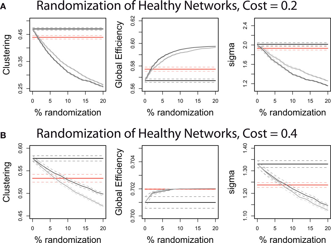
Figure 4. The quantitative properties of the schizophrenic patients’ brain networks can be approximated by randomizing a small proportion of the edges of the controls’ brain networks. Illustrated on graphs with 0.2 topological cost (A) and on graphs with 0.4 topological cost (B), the control networks have 0–20% of their edges randomized. The straight lines show the mean values of the controls (black) and patients (red) in clustering coefficient, global efficiency and small-worldness (sigma). The gray curves show the effect on these network properties of randomizing the control networks: The light gray curves result if the edges are rewired completely at random, whereas the dark gray curves result if the edges are rewired so as to preserve the degree distribution of the original graphs. See Section “Materials and Methods” for explanations of the network measures and the randomization procedures.
The different global network measures are correlated with each other and with the non-graph theoretical measures, as shown in Figure 8. For example, binary global efficiency and robustness are correlated, as are local efficiency and clustering, for both locally and globally thresholded graphs. Weighted global network measures provide complementary results to the binary measures (not shown). Weighted local efficiency is decreased in the schizophrenia population, similar to binary local efficiency. However, weighted global efficiency was higher in the schizophrenic population than in the normal population, a reversal of the finding for binary global efficiency. In fact weighted global efficiency is correlated with weighted local efficiency, average regional strength, and clustering. This indicates that between-group differences in strength or weight of functional connectivity between pairs of regions, rather than differences in topology, are driving the difference in weighted global efficiency.
Modularity
The functional networks of both the patients and the controls have a modular community structure. All of the graphs were significantly more modular than random graphs with the same degree distributions, for the whole cost range of both globally and locally thresholded graphs (not shown). However, there were also quantitative differences in modularity between the groups. See Figure 7 for a representative example of the modular structure of the brain networks and the difference between the groups.
Both the graph theoretical and unsupervised learning approaches provided evidence for relatively reduced modularity in COS networks. Decreased graph theoretical modularity implies that there are relatively less intra-modular edges and more inter-modular edges, compared to what would be expected by chance, in the COS population. For locally thresholded binary graphs, this decrease in modularity occurred at all costs >0.1. For weighted graphs and globally thresholded binary graphs, modularity was also lower in COS, but for a narrower range of costs (Figures 3 and 6A,B). Similar results were found with the unsupervised learning algorithm PAM, which projects brain regions into n-dimensional functional space and groups nearby nodes into the same module. The average silhouette width, which quantifies how well the modules are separated from each other, was lower in the COS population (Figure 6C).
Decreased modularity in the COS population is most clear when the networks are partitioned into fewer than 5 modules. For all the subjects, as more edges are included in the graphs at higher costs, the optimal partitions include fewer modules. On average, modularity is maximized with <5 modules for locally and globally thresholded graphs with costs >0.1 and >0.3 respectively. These are the same costs at which decreased modularity in COS emerges. Consistently, as quantified by decreased average silhouette width, the PAM algorithm finds less modular structure only when the networks are partitioned into less than 5 modules.
In terms of the multi-resolution structure of the graphs as explored with the spin glass algorithm, none of the brain graphs have a clear plateau in their structure, indicating that the modularity of the graphs is not specific to a certain scale. There is group difference in that the graphs of the healthy controls are on average more sensitive to changes in the γ parameter (Figure 6D), separating into a greater number of modules, each of which is composed of fewer nodes on average.
Discussion
The Balance Between Global and Local Connectivity in Schizophrenia
The data suggest the intriguing possibility that COS networks could be less effectively configured for topologically local communication, but better configured for global communication, relative to healthy adolescents, as evidenced by reduced clustering and modularity but greater connectedness, robustness, and global efficiency. Other resting-state fMRI studies of adult-onset schizophrenia have found decreased clustering (Liu et al., 2008) and increased robustness (Lynall et al., 2010). As far as the anatomical foci of the network differences are concerned (Figure 5), Lynall et al. (2010) also found decreased clustering in the superior temporal gyrus and anterior cingulate. Looking to the broader literature on task-activated fMRI, almost all of the brain areas that show decreased regional clustering or increased efficiency in COS – including the insula, the ventral occipital lobe, and the inferior parietal lobule – have been previous implicated in schizophrenia (Glahn et al., 2005; Minzenberg et al., 2009).
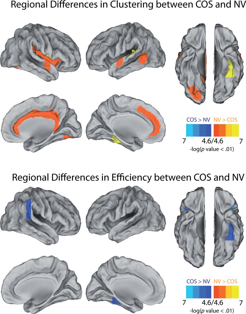
Figure 5. Illustrations of the anatomical foci of decreased clustering and increased global efficiency in schizophrenic (COS) patients relative to controls (NV). At a local threshold of 0.3 topological cost, permutation tests estimated the significance of the differences in regional clustering and efficiency, which are calculated in the same way as the clustering coefficient and the global efficiency, but for each of the 100 nodes individually. Estimations of significance were based on 2000 permutations per region, with p-values corrected for 100 multiple comparisons using a false positive correction p < 1/N = 0.01 Surface representations were created using Caret (http://brainmap.wustl.edu/caret/).
As small-world networks like the human brain are a balance between global and local efficiency (Watts and Strogatz, 1998; Achard et al., 2006), it could be argued that a global optimization process that is crucial for healthy neurodevelopment has been abnormally biased in schizophrenia. Decreased small-worldness, which has also been reported previously in adult-onset schizophrenia (Liu et al., 2008; Lynall et al., 2010), could result if the increase in global efficiency comes at the expense of a disproportionate decrease in clustering. Taken a speculative step further, if an intermediate phenotype with increased global efficiency were evolutionarily favored, this could help explain the persistence of schizophrenia as a disease (Lynall et al., 2010). Admittedly this argument is limited by the fact that while the increase in binary global efficiency is statistically significant, the absolute difference between the groups is quite small. Indeed while decreased clustering in schizophrenia has been replicated in other studies, the story for global efficiency is less clear (Liu et al., 2008; Bassett et al., 2009). Sibling studies will be crucial to better characterize potential intermediate phenotypes.
The shift in the balance between local and global efficiency is consistent with a process of randomization in COS. For all of the network measures that we investigated, the schizophrenic graphs were roughly equivalent to healthy graphs with 5% of the edges randomized (Figures 4A,B). This represents a quantification of what has been previously described as the “subtle randomization” of schizophrenia (Rubinov et al., 2009). Encouragingly it is also testable model for future experiments, because it predicts the direction of the change in schizophrenics relative to controls for any network measure. As network randomization or dedifferentiation has been suggested as an intermediate phenotype for a variety of diseases, it would be very informative to look at the specificity of network properties found in COS, e.g., relative to an ADHD cohort. Randomization of functional network topology is arguably consistent with various neurodevelopmental models of the pathogenesis of schizophrenia, including abnormal axonal growth, synaptic pruning (Feinberg, 1982) or white matter development (Davis et al., 2003). We cannot distinguish between these and other putative developmental mechanisms for abnormal brain network organization based solely on a cross-sectional study of fMRI networks in patients compared to healthy volunteers. However, one potential advantage of using graph theory to describe network organization empirically is that graphical models of network growth or development can be formulated computationally and used to test various competing hypotheses about growth mechanisms driving the formation of the observed network. A classic example of this approach was the demonstration that the observed scale-free degree distribution of the worldwide web could be plausibly explained by a simple growth rule based on preferential attachment (new nodes added to the network tend to become attached preferentially to existing nodes of high degree) (Barabasi and Albert, 1999). In future, it may be possible to use biologically more sophisticated growth models (Goh et al., 2006) to explain the generative developmental mechanisms driving formation of normal and abnormal brain networks.
Modularity
The convergence of our evidence from different methodological approaches points to a disrupted modular organization, with less community structure, in the brain networks of COS patients (Figures 3, 6, and 7). This finding makes sense in the context of a vast literature on the modularity of complex systems, the brain and the mind. As modularity is thought to lessen the potential for error in the construction of complex systems (Simon, 1962), decreased modularity may jeopardize the development of a functional brain network. In theory, a less modular brain would be less able to adapt to multiple and changing goals in the environment (Kashtan and Alon, 2005), predicting cognitive deficits. Decreased topological modularity is also consistent with David’s neurocognitive (1994) hypothesis of dysmodularity in schizophrenia. Of course topological modularity in fMRI networks is not equivalent to neurocognitive modularity. For example, while the relationship between perceptual and attentional systems is crucial to most renditions of the thesis of psychological modularity (Fodor, 1983), our data is agnostic on this issue. David’s account in particular implies that brain systems are hyperconnected in an absolute sense, whereas graph theoretical dysmodularity signifies increased inter-modular connectivity only relative to intra-modular connectivity, and is compatible with the absolute decrease in average connectivity that we also observe in this patient sample. Still, our results provide experimental support for the core prediction of a breakdown of the boundaries between specialized brain systems.
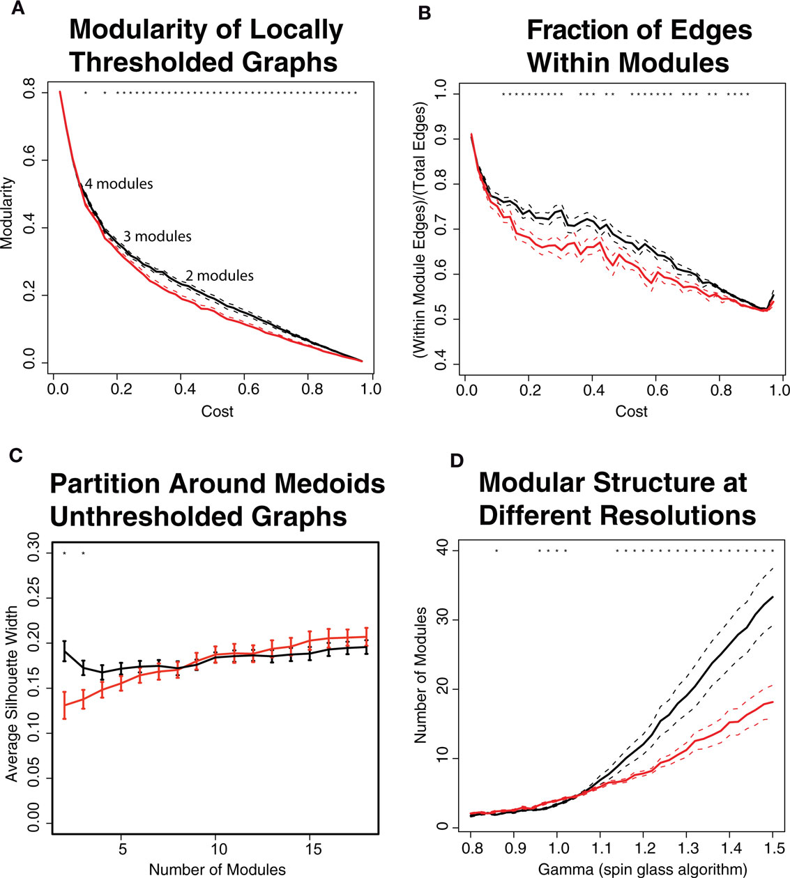
Figure 6. The modular structure of brain networks is disturbed in the childhood-onset schizophrenia (COS) population (red) relative to the control population (black). (A) Modularity is calculated using the fast greedy algorithm on binary, locally thresholded graphs. The COS networks have lower modularity, especially in the range of topological costs where the networks are partitioned into less than 5 modules. (B) The fraction of intra-modular edges, which link nodes in the same module, is decreased in COS. This value is the same as modularity except not normalized by the expected fraction of intra-modular edges. (C) Using the unsupervised learning algorithm Partition Around Medoids (PAM), when the graphs are partitioned into less than 5 modules, the healthy controls have higher modularity as quantified by the average silhouette width. (D) Using a spin glass model with simulated annealing, which looks at the modular structure at different resolutions depending on the gamma parameter, the controls have a wider range of modular structure at different scales.
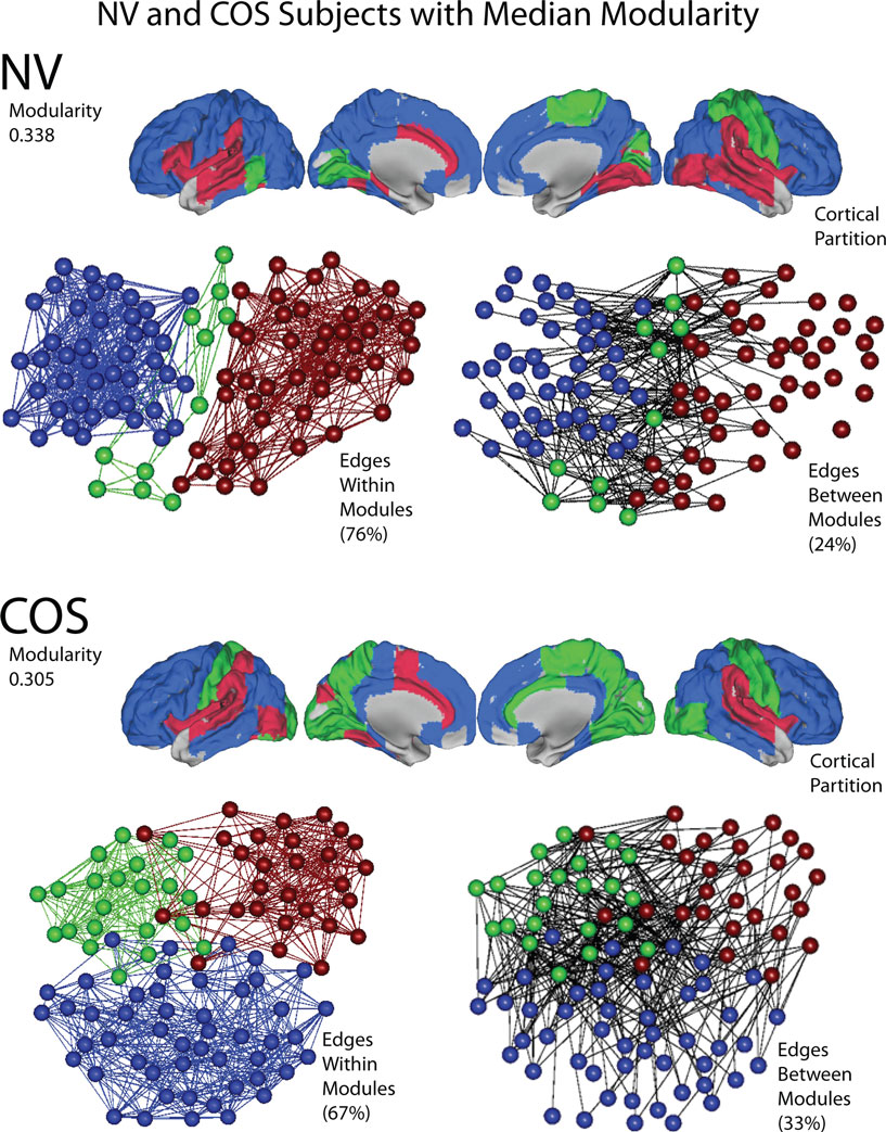
Figure 7. An illustration of modularity, using representative brain networks from the childhood-onset schizophrenia (COS) population and the control (NV) population. At a local threshold of 0.22 topological cost, the modular partition is shown for the median NV subject (above) and the median COS subject (below), in terms of modularity estimated by the fast greedy algorithm. Each module is assigned a specific color, and the modular structure of each subject is illustrated in three different ways: the cortical partition shows the anatomical location of the modules; the left-hand topological plot shows the density of intra-modular edges, between nodes in the same module; and the right-hand topological plot shows the density of inter-modular edges, between nodes in different modules. The layouts of the topological plots are determined by a force-directed algorithm (Fruchterman and Reingold, 1991).
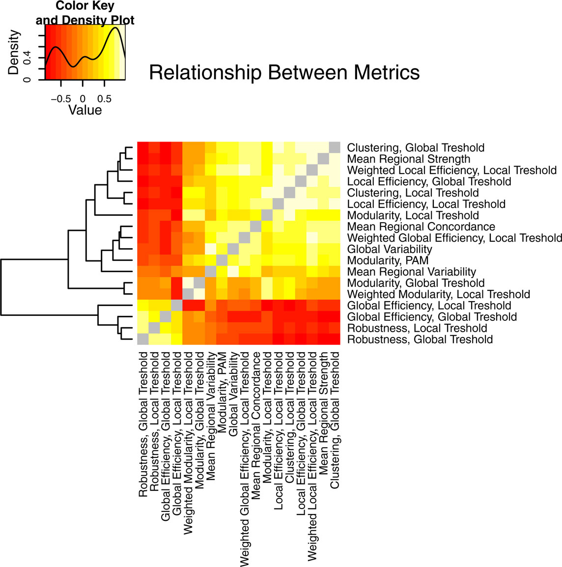
Figure 8. An illustration of the relationship between the different properties of brain networks, including both graph theoretical and non-graph-theoretical metrics. The metrics from Table 1 are correlated between all the subjects in the study and presented as a heat map, with the color value corresponding to the Pearson’s correlation coefficient. The layout is organized by complete linkage hierarchical clustering, according to the dendrogram shown at the left of the figure.
Although differences in modularity have not previously been reported in human brain networks, differences have been found in the modular partition itself, i.e., which brain regions are grouped together into functional communities. For example, Meunier et al. (2009a) found that the brains of a healthy aging population contained more functional modules than younger adults, and Fair et al. (2009) found that during adolescence modules are composed of brain regions that are further apart in physical space. We do not find strong evidence for a group difference in the physical dispersion of brain modules, but it is slightly greater in the controls (not shown). Although the finding that brain networks are modular at multiple resolutions is anticipated by their hierarchical modular organization (Meunier et al., 2009b; Bassett et al., 2010), this is the first study to define modularity across a continuous range of resolutions. Our results may suggest that the modular structure of the functional brain networks is more multi-scale in the healthy controls than the COS population, as reflected by greater sensitivity to the gamma parameter of the spin glass algorithm, but quantifying this hypothesis is an area for future work.
Time Series Statistics
It is unsurprising that in counterpoint to the differences in the complex networks, simpler properties of the MRI time series also differ in COS. The COS population shows decreased internal homogeneity of the MRI signal within anatomical regions, decreased variability of the signal, and decreased average connectivity between anatomical brain regions. Although the exact metric is different, decreased homogeneity of the MRI signal within anatomical regions is consistent with decreased regional homogeneity (ReHo; Zang et al., 2004), which has been reported in some brain regions in an adult-onset schizophrenia population (Liu et al., 2006). The decreases reported with ReHo were for spatial volumes at the scale of a voxel and its nearest neighbors, between 7 and 27 voxels total, so our finding of a decrease of the homogeneity within regions hundreds of voxels in volume is a similar finding at a lower spatial resolution. Decreased regional homogeneity could also be interpreted as yet another aspect of decreased modularity, at a different spatial scale. As for the decreased variability of the global MRI signal, nothing similar has to our knowledge been reported in schizophrenia. A metric called the “resting state activity index” (RSAI), which is ReHo multiplied by the variance of the band-pass filtered time series of a voxel, has been reported as increased in some brain regions in an ADHD cohort (Tian et al., 2008). Our results indicate that this measure would be decreased in COS, although at a different spatial scale.
Finally, decreased average strength or connectivity between anatomical brain regions is a confirmation of a finding in two adult-onset samples (Liu et al., 2008; Lynall et al., 2010). There is a potential link between decreased average strength and topological randomness. Since the connectivity matrices of the graphs are composed of thresholded correlation coefficients, decreased overall connectivity implies that, at a given graph density, there is a lower signal-to-noise ratio in the COS graphs. Assuming that this increased noise is spread equally throughout the nodes, it would be expected to result in increased topological randomness. Topological randomness could also result from other processes, e.g., highly correlated regional time series could result in graphs with the same properties as random graphs. But since our study shows both decreased correlations and increased randomness, it seems likely that they are two sides of the same coin.
Methodological Issues
As the globally thresholded graphs show group differences in connectedness, it would not be implausible for this to drive the differences in other network metrics. The introduction of local thresholding ensures that the disparity between the COS and controls are not due simply to this issue. The known lack of uniformity in the quality of the MR signal from different anatomical regions also makes it reasonable to employ a local threshold, rather than apply the same threshold to regions with different signal-to-noise. The limitations of simply applying a global threshold to a correlation matrix have previously been documented in physics and economics, and several alternatives have been proposed (Onnela et al., 2002; Tumminello et al., 2005; Serrano et al., 2009). Our method is fast, simple, ensures connected graphs, and is defined over the whole cost range. Lacking knowledge of a “true” functional network to provide a gold standard for evaluation of results, it is inappropriate to be too assertive about which graph construction algorithm is best. From a statistical perspective on the individual pairs of time series, we have the most confidence that the edges in a globally thresholded network are genuine functional connections, but the locally thresholded networks have desirable topological constraints and facilitate group comparisons. Side by side contrasts – whether visually on small “model” networks (Figure 1) or in terms of statistical comparisons between groups (Figure 3) – reveal a high degree of similarity in the differently constructed graphs, with some divergence probably due to network fragmentation issues that arise with global thresholding. In addition, for both thresholding schemes, the patient trend in complex network properties is consistent with randomization of a small percentage of the edges in the control networks, as illustrated in Figure 4 for locally thresholded graphs. In short, on the basis of current data, it seems likely that both global and local thresholding rules can be used to construct broadly consistent results but that the between-group comparisons based on local thresholding are simpler to interpret because these networks will all be node-connected by design even at low connection densities. Future studies should attempt to compare these and other methods of graph construction more rigorously using modeled data with known and biologically plausible properties.
Unsupervised learning and graph theoretical algorithms to quantify the community structure of a functional brain network have different strengths and weakness. In the context of fMRI networks, one strength of unsupervised learning algorithms such as partition around medoids (PAM) is that they deal with similarities between objects in n-dimensional space, while graph theory deals with relations between objects. Unsupervised learning methods are thus appropriate to the complete, unthresholded correlation matrix. In contrast graph theoretical approaches allow us to query the community structure of the same, thresholded graphs for which we discuss other network properties. Another difference is that graph theoretical algorithms naturally output an optimum number of modules, which is non-trivial for unsupervised learning algorithms. With PAM, one solution is to maximize the silhouette width over a range of possibilities for the number of modules; this is a potential virtue of PAM compared to hierarchical clustering as it is generally implemented, where the dilemma becomes one of how to cut the dendrogram. In a sense the spin glass algorithm with simulated annealing is intermediate between the two other classes of methods. Similarly to PAM, it can be applied to the unthresholded, weighted graphs, but it also outputs an optimal number of modules, at least for a given value of the gamma parameter. However the inclusion of the gamma parameter, while allowing us to explore the multi-scale modular structure of the graphs, introduces the non-trivial question of which if any scale of description best captures the modular structure. Another serious drawback of the spin glass algorithm is that it is by far the slowest computationally of the 3.
This study is based on a small sample size with short MRI scans. With only 13 COS subjects included, the group differences that we have found will need to be verified in a larger study. In terms of the scans, concatenating two consecutive 3-min scans is probably inferior to having one 6-min scan; however, it would seem comparable to concatenating the interleaved rest blocks from a task-activation study, which has been suggested as acceptable data for a resting-state fMRI study (Fair et al., 2007). In our case, the short consecutive scans are unavoidable, because children and adolescents with severe neuropsychiatric disease often find it difficult to tolerate longer scans. The total acquisition time of 6 min is also quite short, but it has been argued that correlations between brain regions stabilize with even shorter acquisition times (Dijk et al., 2010). The short scanning time does prevent us from looking at very low frequency fluctuations (<0.05 Hz), as the statistical power starts to become quite low.
Conflict of Interest Statement
Edward Bullmore is employed half-time by GlaxoSmithKline and half-time by University of Cambridge.
References
Achard, S., and Bullmore, E. (2007). Efficiency and cost of economical brain functional networks. PLoS Comput. Biol. 3, e17. doi:10.1371/journal.pcbi.0030017.
Achard, S., Salvador, R., Whitcher, B., Suckling, J., and Bullmore, E. (2006). A resilient, low-frequency, small-world human brain functional network with highly connected association cortical hubs. J. Neurosci. 26, 63–72.
Anderson, B., Butts, C., and Carley, K. (1999). The interaction of size and density with graph-level indices. Soc. Networks 21, 239–267.
Bassett, D. S., Bullmore, E., Verchinski, B. A., Mattay, V. S., Weinberger, D. R., and Meyer-Lindenberg, A. (2008). Hierarchical organization of human cortical networks in health and schizophrenia. J. Neurosci. 28, 9239–9248.
Bassett, D. S., Bullmore, E., Meyer-Lindenberg, A., Apud, J. A., Weinberger, D. R., and Coppola, R. (2009). Cognitive fitness of cost-efficient brain functional networks. Proc. Natl. Acad. Sci. U.S.A. 106, 11747–11752.
Bassett, D. S., Greenfield, D., Meyer-Lindenberg, A., Weinberger, D., Moore, S., and Bullmore, E. (2010). Efficient physical embedding of topologically complex information processing networks in brains and computer circuits. PLoS Comput. Biol. 6, e1000748. doi:10.1371/journal.pcbi.1000748.
Bullmore, E., and Sporns, O. (2009). Complex brain networks: graph theoretical analysis of structural and functional systems. Nat. Rev. Neurosci. 10, 1–13.
Burgund, E. D., Kang, H. C., Kelly, J. E., Buckner, R. L., Snyder, A. Z., Petersen, S. E., and Schlaggar, B. L. (2002). The feasibility of a common stereotactic space for children and adults in fMRI studies of development. Neuroimage 17, 184–200.
Cantlon, J. F., Brannon, E. M., Carter, E. J., and Pelphrey, K. A. (2006). Functional imaging of numerical processing in adults and 4-y-old children. PLoS Biol. 4, e125. doi: 10.1371/journal.pbio.0040125.
Chen, Y., Paul, G., Cohen, R., Havlin, S., Borgatti, S. P., Liljeros, F., and Stanley, H. E. (2007). Percolation theory applied to measures of fragmentation in social networks. Phys. Rev. E. Stat. Nonlin. Soft Matter Phys. 75, 046107.
Clauset, A., Newman, M. E. J., and Moore, C. (2004). Finding community structure in very large networks. Phys. Rev. E. Stat. Nonlin. Soft Matter Phys. 70, 066111.
Cordes, D., Haughton, V., Carew, J. D., Arfanakis, K., and Maravilla, K. (2002). Hierarchical clustering to measure connectivity in fMRI resting-state data. Magn. Reson. Imaging 20, 305–317.
Cox, R. W. (1996). AFNI: software for analysis and visualization of functional magnetic resonance neuroimages. Comput. Biomed. Res. 29, 162–173.
Crone, E. A., Wendelken, C., Donohue, S., van Leijenhorst, L., and Bunge, S. A. (2006). Neurocognitive development of the ability to manipulate information in working memory. Proc. Natl. Acad. Sci. U.S.A. 103, 9315–9320.
Csardi, G., and Nepusz, T. (2006). The igraph software package for complex network research. InterJournal Complex Syst. Article No. 1695.
David, A. S. (1994). Dysmodularity: a neurocognitive model for schizophrenia. Schizophr. Bull. 20, 249–255.
Davis, K. L., Stewart, D. G., Friedman, J. I., Buchsbaum, M., Harvey, P. D., Hof, P. R., Buxbaum, J., and Haroutunian, V. (2003). White matter changes in schizophrenia: evidence for myelin-related dysfunction. Arch. Gen. Psychiatry 60, 443–456.
Dijk, K. R. A. V., Hedden, T., Venkataraman, A., Evans, K. C., Lazar, S. W., and Buckner, R. L. (2010). Intrinsic functional connectivity as a tool for human connectomics: theory, properties, and optimization. J. Neurophysiol. 103, 297–321.
Dorogovtsev, S., Goltsev, A., and Mendes, J. (2008). Critical phenomena in complex networks. Rev. Mod. Phys. 80, 1275.
Durston, S., Tottenham, N. T., Thomas, K. M., Davidson, M. C., Eigsti, I. M., Yang, Y., Ulug, A. M., and Casey, B. J. (2003). Differential patterns of striatal activation in young children with and without ADHD. Biol. Psychiatry 53, 871–878.
Eppstein, D., Paterson, M., and Yao, F. (1992). On nearest-neighbor graphs. Lect. Notes Comput. Sci. 623, 416–426.
Fair, D. A., Cohen, A. L., Power, J. D., Dosenbach, N. U. F., Church, J. A., Miezin, F. M., Schlaggar, B. L., and Petersen, S. E. (2009). Functional brain networks develop from a “local to distributed” organization. PLoS Comput. Biol. 5, e1000381. doi: 10.1371/journal.pcbi.1000381.
Fair, D. A., Schlaggar, B. L., Cohen, A. L., Miezin, F. M., Dosenbach, N. U. F., Wenger, K. K., Fox, M. D., Snyder, A. Z., Raichle, M. E., and Petersen, S. E. (2007). A method for using blocked and event-related fMRI data to study “resting state” functional connectivity. Neuroimage 35, 396–405.
Feinberg, I. (1982). Schizophrenia: caused by a fault in programmed synaptic elimination during adolescence? J. Psychiatr. Res. 17, 319–334.
Fodor, J. A. (1983). The Modularity of Mind: An Essay on Faculty Psychology. Cambridge, MA: MIT Press.
Fortunato, S., and Barthélemy, M. (2007). Resolution limit in community detection. Proc. Natl. Acad. Sci. U.S.A. 104, 36–41.
Fruchterman, T. M. J., and Reingold, E. M. (1991). Graph drawing by force-directed placement. Softw. Pract. Exper. 21, 1129–1164.
Galvan, A., Hare, T. A., Parra, C. E., Penn, J., Voss, H., Glover, G., and Casey, B. J. (2006). Earlier development of the accumbens relative to orbitofrontal cortex might underlie risk-taking behavior in adolescents. J. Neurosci. 26, 6885–6892.
Giedd, J. N., Lalonde, F. M., Celano, M. J., White, S. L., Wallace, G. L., Lee, N. R., and Lenroot, R. K. (2009). Anatomical brain magnetic resonance imaging of typically developing children and adolescents. J. Am. Acad. Child Adolesc. Psychiatry 48, 465–470.
Glahn, D. C., Ragland, J. D., Abramoff, A., Barrett, J., Laird, A. R., Bearden, C. E., and Velligan, D. I. (2005). Beyond hypofrontality: a quantitative meta-analysis of functional neuroimaging studies of working memory in schizophrenia. Hum. Brain Mapp. 25, 60–69.
Gogtay, N., Lu, A., Leow, A. D., Klunder, A. D., Lee, A. D., Chavez, A., Greenstein, D., Giedd, J. N., Toga, A. W., Rapoport, J. L., and Thompson, P. M. (2008). Three-dimensional brain growth abnormalities in childhood-onset schizophrenia visualized by using tensor-based morphometry. Proc. Natl. Acad. Sci. U.S.A. 105, 15979–15984.
Goh, K. I., Salvi, G., Kahng, B., and Kim, D. (2006). Skeleton and fractal scaling in complex networks. Phys. Rev. Lett. 96, 018701.
Guimerà, R., Sales-Pardo, M., and Amaral, L. A. N. (2004). Modularity from fluctuations in random graphs and complex networks. Phys. Rev. E. Stat. Nonlin. Soft Matter Phys. 70, 025101.
Hagmann, P., Cammoun, L., Gigandet, X., Meuli, R., Honey, C. J., Wedeen, V. J., and Sporns, O. (2008). Mapping the structural core of human cerebral cortex. PLoS Biol. 6, e159. doi:10.1371/journal.pbio.0060159.
Heimo, T., Kumpula, J., Kaski, K., and Saramaki, J. (2008). Detecting modules in dense weighted networks with the potts method. J. Stat. Mech. Theory Exp. 2008, 08007.
Humphries, M. D., Gurney, K., and Prescott, T. J. (2006). The brainstem reticular formation is a small-world, not scale-free, network. Proc. Biol. Sci. 273, 503–511.
Jenkinson, M., Bannister, P., Brady, M., and Smith, S. (2002). Improved optimization for the robust and accurate linear registration and motion correction of brain images. Neuroimage 17, 825–841.
Jenkinson, M., and Smith, S. (2001). A global optimisation method for robust affine registration of brain images. Med. Image Anal. 5, 143–156.
Kang, H. C., Burgund, E. D., Lugar, H. M., Petersen, S. E., and Schlaggar, B. L. (2003). Comparison of functional activation foci in children and adults using a common stereotactic space. Neuroimage 19, 16–28.
Kashtan, N., and Alon, U. (2005). Spontaneous evolution of modularity and network motifs. Proc. Natl. Acad. Sci. U.S.A. 102, 13773–13778.
Kaufman, L., and Rousseeuw, P. (1987). “Clustering by means of medoids,” in Statistical Data Analysis Based on the L1-Norm and Related Methods, ed. Y. Dodge (Berlin: Birkhäuser), 405–416.
Kruskal, J. B. (1956). On the shortest spanning subtree of a graph and the traveling salesman problem. Proc. Am. Math. Soc. 7, 48–50.
Latora, V., and Marchiori, M. (2001). Efficient behavior of small-world networks. Phys. Rev. Lett. 87, 198701.
Lee, J., Folley, B. S., Gore, J., and Park, S. (2008). Origins of spatial working memory deficits in schizophrenia: an event-related fMRI and near-infrared spectroscopy study. PLoS ONE 3, e1760. doi:10.1371/journal.pone.0001760.
Liu, H., Liu, Z., Liang, M., Hao, Y., Tan, L., Kuang, F., Yi, Y., Xu, L., and Jiang, T. (2006). Decreased regional homogeneity in schizophrenia: a resting state functional magnetic resonance imaging study. Neuroreport 17, 19–22.
Liu, Y., Liang, M., Zhou, Y., He, Y., Hao, Y., Song, M., Yu, C., Liu, H., Liu, Z., and Jiang, T. (2008). Disrupted small-world networks in schizophrenia. Brain 131, 945–961.
Lynall, M.-E., Bassett, D. S., Kerwin, R., McKenna, P. J., Kitzbichler, M., Muller, U., and Bullmore, E. (2010). Functional connectivity and brain networks in schizophrenia. J. Neurosci. 30, 9477–9487.
Meunier, D., Achard, S., Morcom, A., and Bullmore, E. (2009a). Age-related changes in modular organization of human brain functional networks. Neuroimage 44, 715–723.
Meunier, D., Lambiotte, R., Fornito, A., Ersche, K. D., and Bullmore, E. (2009b). Hierarchical modularity in human brain functional networks. Front. Neuroinformatics 3:37. doi: 10.3389/neuro.11.037.2009.
Milo, R., Kashtan, N., Itzkovitz, S., Newman, M., and Alon, U. (2004). On the uniform generation of random graphs with prescribed degree sequences. arXiv:0312028v2.
Minzenberg, M. J., Laird, A. R., Thelen, S., Carter, C. S., and Glahn, D. C. (2009). Meta-analysis of 41 functional neuroimaging studies of executive function in schizophrenia. Arch. Gen. Psychiatry 66, 811–822.
Newman, M. E. J., and Girvan, M. (2004). Finding and evaluating community structure in networks. Phys. Rev. E. Stat. Nonlin. Soft Matter Phys. 69, 026113.
Onnela, J.-P., Chakraborti, A., Kaski, K., and Kertiész, J. (2002). Dynamic asset trees and portfolio analysis. Eur. Phys. J. B. 30, 285–288.
Percival, D. B., and Walden, A. T. (2006). Wavelet Methods for Time Series Analysis. Cambridge, UK: Cambridge University Press.
Pessoa, V. F., Monge-Fuentes, V., Simon, C. Y., Suganuma, E., and Tavares, M. C. H. (2008). The Müller-Lyer illusion as a tool for schizophrenia screening. Rev. Neurosci. 19, 91–100.
Prim, R. C. (1957). Shortest connection networks and some generalizations. Bell Syst. Tech. J. 36, 1389–1401.
R Development Core Team (2009). R: A Language and Environment for Statistical Computing. Vienna: R Foundation for Statistical Computing. Available at http://www.R-project.org.
Reichardt, J., and Bornholdt, S. (2006). Statistical mechanics of community detection. Phys. Rev. E. Stat. Nonlin. Soft Matter Phys. 74, 016110.
Rubinov, M., Knock, S. A., Stam, C. J., Micheloyannis, S., Harris, A. W. F., Williams, L. M., and Breakspear, M. (2009). Small-world properties of nonlinear brain activity in schizophrenia. Hum. Brain Mapp. 30, 403–416.
Salvador, R., Suckling, J., Coleman, M. R., Pickard, J. D., Menon, D., and Bullmore, E. (2005). Neurophysiological architecture of functional magnetic resonance images of human brain. Cereb. Cortex 15, 1332–1342.
Schank, T., and Wagner, D. (2004). Approximating clustering-coefficient and transitivity. J. Graph Algorithms Appl. 9, 265–275.
Serrano, M. A., Boguñá, M., and Vespignani, A. (2009). Extracting the multiscale backbone of complex weighted networks. Proc. Natl. Acad. Sci. U.S.A. 106, 6483–6488.
Shapleske, J., Rossell, S. L., Chitnis, X. A., Suckling, J., Simmons, A., Bullmore, E. T., Woodruff, P. W. R., and David, A. S. (2002). A computational morphometric MRI study of schizophrenia: effects of hallucinations. Cereb. Cortex 12, 1331–1341.
Sheskin, D. J. (2007). Handbook of Parametric and Nonparametric Statistical Procedures, 4th Edn. Boca Raton, FL: CRC Press.
Smith, S. M., Jenkinson, M., Woolrich, M. W., Beckmann, C. F., Behrens, T. E. J., Johansen-Berg, H., Bannister, P. R., Luca, M. D., Drobnjak, I., Flitney, D. E., Niazy, R. K., Saunders, J., Vickers, J., Zhang, Y., Stefano, N. D., Brady, J. M., and Matthews, P. M. (2004). Advances in functional and structural MR image analysis and implementation as FSL. Neuroimage 23(Suppl. 1), S208–S219.
Tian, L., Jiang, T., Liang, M., Zang, Y., He, Y., Sui, M., and Wang, Y. (2008). Enhanced resting-state brain activities in ADHD patients: a fMRI study. Brain Dev. 30, 342–348.
Tumminello, M., Aste, T., Matteo, T. D., and Mantegna, R. N. (2005). A tool for filtering information in complex systems. Proc. Natl. Acad. Sci. U.S.A. 102, 10421–10426.
Turkeltaub, P. E., Gareau, L., Flowers, D. L., Zeffiro, T. A., and Eden, G. F. (2003). Development of neural mechanisms for reading. Nat. Neurosci. 6, 767–773.
Venables, W. N., and Ripley, B. D. (2002). Modern Applied Statistics with S, 4th Edn. New York: Springer.
Watts, D. J., and Strogatz, S. H. (1998). Collective dynamics of “small-world” networks. Nature 393, 440–442.
Keywords: graph theory, brain, network, modularity, schizophrenia, clustering, fMRI
Citation: Alexander-Bloch AF, Gogtay N, Meunier D, Birn R, Clasen L, Lalonde F, Lenroot R, Giedd J and Bullmore ET (2010) Disrupted modularity and local connectivity of brain functional networks in childhood-onset schizophrenia. Front. Syst. Neurosci. 4:147. doi: 10.3389/fnsys.2010.00147
Received: 14 June 2010;
Paper pending published: 25 July 2010;
Accepted: 10 September 2010;
Published online: 08 October 2010.
Edited by:
Silvina G. Horovitz, National Institutes of Health, USAReviewed by:
Barry Horwitz, National Institutes of Health, USAMalle A. Tagamats, University of Maryland, USA
Copyright: © 2010 Alexander-Bloch, Gogtay, Meunier, Birn, Clasen, Lalonde, Lenroot, Giedd and Bullmore. This is an open-access article subject to an exclusive license agreement between the authors and the Frontiers Research Foundation, which permits unrestricted use, distribution, and reproduction in any medium, provided the original authors and source are credited.
*Correspondence: Edward T. Bullmore, Department of Psychiatry, University of Cambridge, Herchel Smith Building, Cambridge Biomedical Campus, Cambridge CB2 0SZ, UK. e-mail: etb23@cam.ac.uk