 Haoran Gao1
 Junxian He1
 Haibing Wang1
 Tengxiao Wang1
 Zhengqing Zhong1
 Jianyi Yu1
 Ying Wang2
 Min Tian1
 Cong Shi1*
- 1The School of Microelectronics and Communication Engineering, Chongqing University, Chongqing, China
- 2State Key Laboratory of Computer Architecture, Institute of Computing Technology, Chinese Academy of Sciences, Beijing, China
Spiking neural networks (SNNs) have attracted intensive attention due to the efficient event-driven computing paradigm. Among SNN training methods, the ANN-to-SNN conversion is usually regarded to achieve state-of-the-art recognition accuracies. However, many existing ANN-to-SNN techniques impose lengthy post-conversion steps like threshold balancing and weight renormalization, to compensate for the inherent behavioral discrepancy between artificial and spiking neurons. In addition, they require a long temporal window to encode and process as many spikes as possible to better approximate the real-valued ANN neurons, leading to a high inference latency. To overcome these challenges, we propose a calcium-gated bipolar leaky integrate and fire (Ca-LIF) spiking neuron model to better approximate the functions of the ReLU neurons widely adopted in ANNs. We also propose a quantization-aware training (QAT)-based framework leveraging an off-the-shelf QAT toolkit for easy ANN-to-SNN conversion, which directly exports the learned ANN weights to SNNs requiring no post-conversion processing. We benchmarked our method on typical deep network structures with varying time-step lengths from 8 to 128. Compared to other research, our converted SNNs reported competitively high-accuracy performance, while enjoying relatively short inference time steps.
1. Introduction
Deep learning technology has achieved unprecedented success in versatile intelligent applications in modern society. However, the real-valued deep artificial neural network (ANN) models are quite power-hungry due to their intensive matrix multiplication operations (LeCun et al., 2015). By contrast, neuromorphic computing with spiking neural networks (SNNs) is more promising for ubiquitous cost- and energy-constrained mobile, embedded, and edge platforms (Roy et al., 2019). The SNN adopts spatiotemporally sparse spike events to encode, transmit, and process information the way human brain cortical neurons do.
However, training deep SNNs is highly challenging because it is difficult to directly apply the backpropagation (BP) method to SNNs owing to the inherent discontinuity of discrete spikes. A common indirect approach to overcome this problem is to train a structurally equivalent ANN model offline and then convert it to an SNN with the learned synaptic weights for inference, where the real values of inputs and outputs of ANN neurons correspond to the rates of presynaptic (input) and postsynaptic (output) spikes of the SNN neurons (Diehl et al., 2015; Hunsberger and Eliasmith, 2016; Rueckauer et al., 2017; Zhang et al., 2019; Han and Roy, 2020; Han et al., 2020; Kim et al., 2020; Lee et al., 2020; Yang et al., 2020; Deng and Gu, 2021; Dubhir et al., 2021; Ho and Chang, 2021; Hu et al., 2021; Kundu et al., 2021; Li et al., 2021b; Bu et al., 2022; Liu et al., 2022). Although previous ANN-to-SNN techniques usually obtain state-of-the-art object recognition accuracies, they require complicated post-conversion fixations such as threshold balancing (Diehl et al., 2015; Rueckauer et al., 2017; Han et al., 2020; Liu et al., 2022), weight normalization (Diehl et al., 2015; Rueckauer et al., 2017; Ho and Chang, 2021), spike-norm (Sengupta et al., 2019), and channel-wise normalization (Kim et al., 2020), to compensate the behavioral discrepancies between artificial and spiking neurons. In addition, a few of those methods require a relatively long time window (e.g)., 2,500 algorithmic discrete time steps (Sengupta et al., 2019), allowing for sufficient spike emissions to precisely represent the real values of the equivalent ANNs. This incurs high latencies and additional computational overheads, severely compromising the efficiency of SNNs.
To mitigate the aforementioned overheads in ANN-to-SNN conversion, this study proposes a simple and effective deep ANN-to-SNN framework without any post-conversion tuning, and the converted SNN can achieve a high recognition accuracy in a relatively shorter temporal window (i.e., 128 down to 8 time steps). This framework adopts our proposed calcium-gated bipolar leaky integrate and fire (Ca-LIF) spiking neuron model to well approximate the function of the ReLU neuron widely used in deep ANNs. It fully leverages off-the-shelf quantization-aware training (QAT) toolkit to train the ANNs with low-bit precision ReLU activations, which can be captured as the spike rate of the Ca-LIF neuron in an intermediately short time window.
The rest of this article is organized as follows: Section 2 explains the background of neural networks, including the ReLU and the basic LIF neurons. Section 3 proposes our Ca-LIF spiking neuron model and the QAT-based ANN-to-SNN framework, which are validated with elaborate experiments mentioned in Section 4. Section 5 summarizes this study.
2. Preliminaries
2.1. Convolution neural network
The typical structure of a deep neural network (shown in Figure 1) is composed of alternating convolutional (CONV) layers for feature detection and pooling layers for dimensionality reduction, followed by stacked fully connected (FC) layers as a feature classifier. In a CONV layer, each neuron in a channel is connected via a shared weight kernel to a few neurons within a spatial neighborhood called receptive field (RF) in the channels of the precedent layer. In a pooling layer, each neuron aggregates the outputs of the neurons in a p × p spatial window from the corresponding channel of its precedent CONV layer, thereby realizing data dimensionality reduction and small translational invariance. In an FC layer, each neuron is fully connected to all neurons in its precedent layer. The neuron with the most active outputs in the final layer indicates the recognition result.
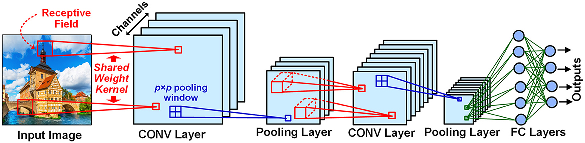
Figure 1. Typical structure of deep neural networks. In convolutional (CONV) layers, the Receptive Field (RF) is a spatial neighborhood around a neuron in a channel connected by a shared weight kernel to the next layer's neurons. The pooling layer is utilized to reduce the size of its preceding CONV layer feature map by a pooling window. Each neuron in a fully connected (FC) layer are connected to all the neurons in its previous layer. The outputs of the final layer indicate the image object recognition result.
2.2. ReLU neuron in ANN
The output of the ReLU neuron widely used in ANNs is formulated as follows:
where z is the net summation which is calculated as follows:
with xi as the i-th input value to the neuron, wi the connecting weight, and b a bias term. Figure 2A depicts the ReLU function.
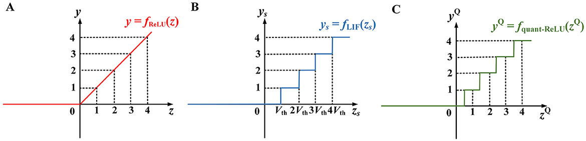
Figure 2. Input–output relationships of (A) the ReLU neuron, (B) the basic LIF neuron, and (C) the quantized ReLU approximation based on rounding (Deng and Gu, 2021). In (A), when the input z > 0, the output y = z, otherwise y = 0. In (B), zS is the integrated membrane across the total time steps and Vth is the threshold. In (C), zQ, yQ are the input and output of the quantized ReLU function based on rounding.
2.3. Basic LIF neuron in SNN
The LIF neuron is the most commonly adopted model in SNNs (Roy et al., 2019). It is biologically plausible with an internal state variable called membrane potential Vm (initialized to 0 at the beginning of spike trains of every input image) and exhibits rich temporal dynamics. Once the neuron receives a spike event via any of its synapses, the corresponding synaptic weight wi is integrated into its Vm. Meanwhile, the neuron linearly leaks all the time. The event-driven LIF model can be described as follows:
where tk and i(k) are the algorithmic discrete time step and the index of the synapse when and where the k-th input presynaptic spike arrives, respectively, and λ is a constant leakage at every time step. Whenever Vm crosses a pre-defined threshold Vth > 0, the neuron fires a postsynaptic spike to its downstream neurons and resets Vm by subtracting Vth from it. Suppose an input image has a presentation window of T time steps (i.e., the length of spike trains encoded from the image pixels), one would estimate the total output spike count of the LIF neuron as follows (Han et al., 2020; Lee et al., 2020):
where floor returns the largest integer no larger than its argument, and zs is the net integration across all the T time steps:
with xsi being the total count of input spikes via synapse i. Equation (3a) is depicted in Figure 2B.
3. Materials and methods
3.1. Motivation
From the similarities between Eqs. (1) and (3) and between Figures 2A, B, it appears that the LIF neuron can be used to approximate the ReLU function by treating its pre- and postsynaptic spike rates or counts xsi, ys as ReLU's input and output values xi, y. The leakage term -λT in Equation (3b) acts as the bias b in Equation (1b). Thus, we can first train a deep ANN using standard BP, and then export the learned weights and biases to a structurally equivalent SNN of LIF neurons for inference.
However, there are three challenges hindering such a direct ANN-to-SNN conversion:
1) The input and output spike counts of the LIF neuron are discrete integers, while ReLU allows continuous-valued inputs and output. Particularly, the ys in Figure 2B is a scaled (by the factor of 1/Vth) and staircase-like approximation of the ReLU output y in Figure 2A. To reduce their discrepancy, a long time window is often needed to generate sufficient output spikes, resulting in a high inference latency.
2) Due to the extra temporal dimension of the LIF neuron, Equation (3a) may be significantly violated sometimes. As illustrated in Figure 3, the earlier input spikes via positive synaptic weights trigger output spikes, which could not be canceled out by later input spikes via more negative synaptic weights, as the information accumulated into the negative Vm of the LIF neuron cannot be passed on to other neurons via any output spikes. Therefore, even when the LIF neuron has weights and inputs values xsi = xi identical to those of the ReLU neuron, with a leakage constant set to be λ = -b/T, LIF output spike count ys still severely deviates from ReLU output y and largely violates Equation (3a).
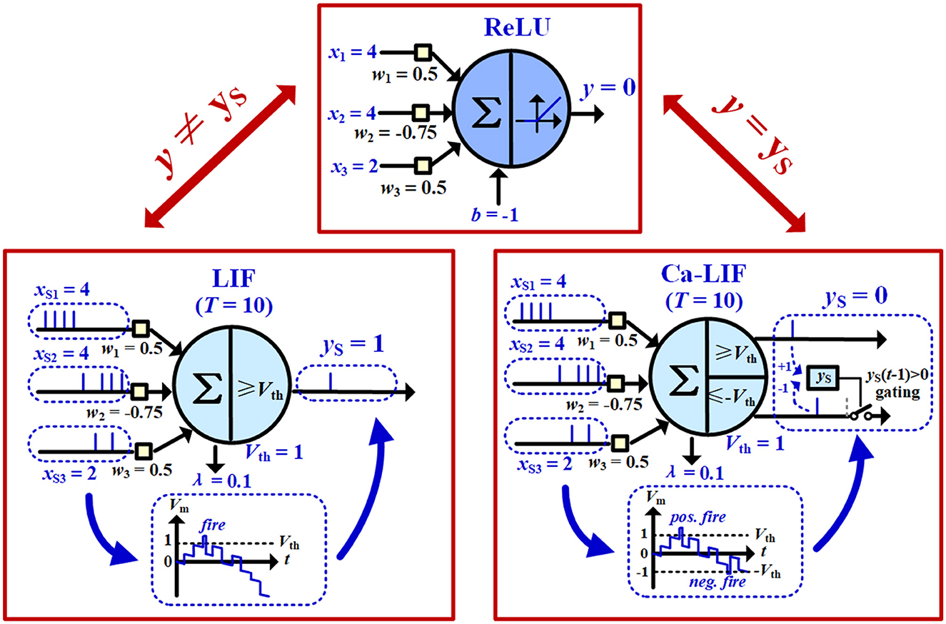
Figure 3. Comparison of the input–output relationships of the ReLU neuron, the basic LIF neuron, and the proposed Ca-LIF neuron.
3) Note that there is a floor(zs/Vth) operation in Equation (3a) due to the discrete fire thresholding mechanism, leading to a shift of Vth/2 along the positive zs axis in Figure 2B, compared to the rounding-based quantized ReLU approximation as shown in Figure 2C (Deng and Gu, 2021). Indeed, a better approximation to the ReLU neuron expects a round operation instead of the floor function to obtain statistically zero-mean quantization errors (Deng and Gu, 2021).
To overcome the first challenge, we can leverage QAT ANN training toolkits to produce an ANN with low-precision ReLU outputs, while minimizing the accuracy loss compared to a full-precision ANN. The complete QAT-based ANN-to-SNN framework is proposed in Section 3.3. For the other two challenges, we propose a Ca-LIF neuron model. It reserves the spike-based event-driven nature of a biological neuron, while mathematically better aligning with the (quantized) ReLU curve regardless of the input spike arrival order, as introduced later.
3.2. The proposed Ca-LIF spiking neuron model
We proposed the Ca-LIF spiking neuron model to correct the output mismatches between the basic LIF model and the quantized ReLU function, as exhibited in Figure 3. It performs the same leaking and integration operations as in Equation (2) but employs a slightly different firing mechanism. The Ca-LIF neuron holds symmetric thresholds Vth > 0 and -Vth < 0. Once its Vm up-crosses Vth, or down-crosses -Vth with the gating condition yS(t-1) > 0 satisfied, the neuron fires a positive or negative spike, respectively, where yS in the Ca-LIF neuron represents signed output of the spike count. i.e., the positive output spike count minus the positive negative spike count. Actually, ys resembles the calcium ion concentration (Ca+) in a biological neuron (Brader et al., 2007). Note that if a Ca-LIF neuron receives a negative spike sent by another neuron via its synapse i, -wi is instead integrated onto the Vm in Equation (2). This neuron resets by adding Vth to the Vm after it fires a negative output spike.
Moreover, as mentioned earlier, the spiking neuron should perform a rounding function to replace the floor operation on (zs/Vth) in Equation (3a) to better align with the quantized ReLU behavior. Mathematically, the Ca-LIF neuron should execute:
To achieve this, after all the spike events input to the SNN composed of Ca-LIF neurons have been processed, each Ca-LIF neuron in the first SNN layer with their Vm between Vth/2 ~ Vth (or between -Vth ~ -Vth/2, and yS > 0) is a force to fire a positive (or negative) spike. These rounding spikes propagate to other Ca-LIF neurons in subsequent layers, trying to trigger their own rounding spikes based on their halved thresholds ±Vth/2. This progresses until the final layer is completed.
3.3. QAT-based ANN-to-SNN conversion framework
Using the aforementioned Ca-LIF neurons, we now propose the details of the simple QAT-based ANN-to-SNN conversion framework. First, utilize any off-the-shelf QAT toolkit available to train a deep quantized ANN. Next, export the learned ANN weights to an SNN composed of Ca-LIF neurons organized in the same network structure as the ANN, and analytically determine the neuron thresholds. Typically, a QAT toolkit would provide the low-bit precision mantissa associated with a scaling factor Sw of each learned quantized weight in the ANN, as well as the bias b, the input and output scaling factors Sx and Sy of the neurons. One quantized ReLU neuron performs inference with its such learned parameters as follows:
Wherein the superscript Q denotes quantized. By comparing the forms of Equations (3c) and (4), it can be found that, if we simply set
for a Ca-LIF neuron, it can seamlessly replace the quantized ReLU neuron and reproduce its input–output relationship of Figure 2C in the form of spike counts, with exactly the same learned weights.
In addition, one neuron in an average pooling layer of the quantized ANN performs a quantized linear operation as follows:
where PW denotes the set of ReLU neurons in the p × p pooling window connecting to the pooling neuron. Such pooling neuron can also be approximated by our Ca-LIF neuron but without the ys gating constraint on negative firing, and with its Vth being p2, the leakage constant λ being 0, and all synaptic weights being 1.
4. Experiments
4.1. Benchmark datasets
We evaluated our method on five image datasets: MNIST, CIFAR-10, CIFAR-100, Caltech-101, and Tiny-ImageNet. Their image resolution, number of object categories, as well as the training/testing subsets partition are listed in Table 1. The MNIST dataset contains 28 × 28 handwritten digit images of 10 classes, i.e., 0–9. It is divided into 50,000 training samples and 10,000 testing samples. The CIFAR-10 dataset contains 10 object classes, including 50,000 training images and 10,000 testing images with an image size of 32 × 32. For CIFAR-100, it holds 100 object classes, each owning 500 training samples and 100 testing samples. The Caltech-101 dataset consists of 101 object categories, each of which holds 40–800 image samples with a size of 300 × 200 pixels. The Tiny-ImageNet benchmark is composed of as many as 200 object classes, each of which has 500 training samples and 50 testing samples with an image size of 64 × 64.
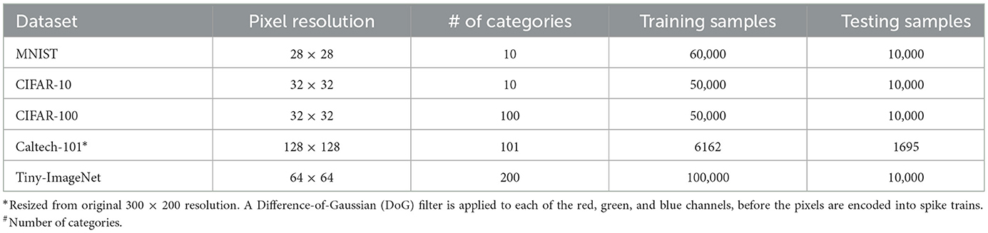
Table 1. Benchmark datasets.
We employed the inter-spike interval (ISI) coding method (Guo et al., 2021) to encode pixel values into spikes. The pixel brightness Pix (for color images, this refers to the color component in each of the red, green, and blue channels) was converted to a spike train with N spikes in a T time-step window, with N = floor(α · T· Pix / Pix_max), where function floor(x) returned the biggest integer no larger than x, Pix_max was the maximum value a pixel could reach (for 8-bit image pixels which used in our work, Pix_max = 255), and α ≤ 1 controlled the spike rate, which was set to 1 throughout our experiments unless otherwise stated. The n-th spike happened at time step tn = floor(n · tint), where tint = T / (α· T· Pix / Pix_max) = Pix_max / (α·Pix) ≥ 1 was the temporal interval (non-rounded) between two successive spikes. In particular, the brightest pixel value of 255 would be converted to a spike train of totally N = floor(α· T · 255/255) = T spikes with tint = α = 1. In other words, its converted spike train reached the maximum rate of one spike per time step.
4.2. Network structure configuration
We adopted five typical deep network structures to evaluate our Ca-LIF spiking neuron and ANN-to-SNN framework: (1) Lenet-5 (Lecun et al., 1998), (2) VGG-9 (Lee et al., 2020), (3) ResNet-11H, which only kept half of the channels in each CONV layer of the Resnet-11 (Lee et al., 2020), and (4) MobileNet-20, a reduced version of MobileNetV1 (Howard et al., 2017) with the original 16th – 23rd CONV layers removed, and (5) VGG-16. We modified all pooling layers in these networks to perform average pooling. Moreover, for each network, the kernel size in its first layer and the number of neurons in its last FC layer had to accommodate the image size (i.e., the image resolution and number of color channels) and the number of object categories, respectively, when coping with different image datasets.
4.3. Recognition accuracy
In our experiments, we leveraged the off-the-shelf PyTorch QAT toolkit (PyTorch Foundation, 2022) to train deep ANNs of the aforementioned five neural network structures, and then exported the learned parameters to construct structurally equivalent SNNs for inference. The learned weights were directly translated to the synaptic weights of SNN Ca-LIF neurons, while other parameters like the biases and quantization scaling factors were used to determine the thresholds and leakages of Ca-LIF neurons according to Equation (5).
The PyTorch QAT toolkit quantized the inputs, outputs, and weights of the ANN neurons all into a signed 8-bit format during training. Note that we can freely leverage any other available QAT toolkit supporting other ANN activation bit-precisions, including binary and ternary activations. We employed the standard stochastic gradient descent method to train ANNs with a momentum of 0.9. The batch normalization (BN) (Ioffe and Szegedy, 2015) technique was also employed in the QAT training to improve the accuracy performance of some deep networks on complex datasets. The BN layers' parameters were updated with other parameters in a unified QAT process and were already incorporated into the convolution layers' biases and quantized 8-bit weights before being exported to SNNs. The training of the QAT starts from scratch rather than relying on transferring learning. For converted SNN inference, we set T = 128 time steps as the baseline spike encoding window length. The testing accuracies of the SNN (T = 128) under each network structure configuration in Section 4.2 are demonstrated in Figure 4. These results indicated that our ANN-to-SNN conversion framework along with the proposed Ca-LIF neuron model achieved competitively high recognition performance. Indeed, the accuracy gap of the converted SNNs (T = 128) and their pre-conversion quantized ANN counterparts was negligibly below 0.04%. The results of experiments on MNIST, CIFAR-10, CIFAR-100, Caltech-101, and Tiny-ImageNet demonstrate the superiority and universality of our method.
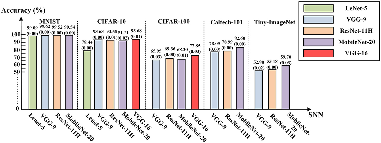
Figure 4. The testing accuracies of the SNNs (T = 128) converted from quantized ANNs. The numeric in the bracket below the accuracy is the loss of the converted SNN compared with the corresponding quantized ANN.
Moreover, to evaluate the accuracy vs. latency (i.e., the number of inference time steps) tradeoff of our converted SNNs, Figure 5 depicts the accuracies of our converted VGG-16 SNN on the CIFAR-10 and CIFAR-100 image datasets under different time window length configurations with varying time steps of T = 8 to 512. The accuracies saturate above T = 128, as we utilized a signed 8-bit activation for the pre-conversion quantized ANN. A more elaborate work comparison and discussion about this is provided in Section 4.4.
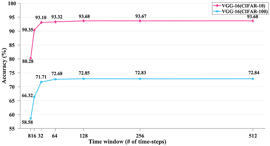
Figure 5. The inference accuracy performance of the converted VGG-16 SNN on the CIFAR-10 and CIFAR-100 datasets using varying numbers of time-steps.
4.4. Work comparison and discussion
Table 2 compares our work with other previous ANN-to-SNN conversion research. Since a quantized ANN itself may suffer a bit lower accuracy (sometimes a little higher) than its full-precision version, we also trained and tested the recognition accuracies of full-precision ANNs using the aforementioned network structures for a fair comparison, and further evaluated the accuracy loss between the converted SNNs and corresponding full-precision ANNs.
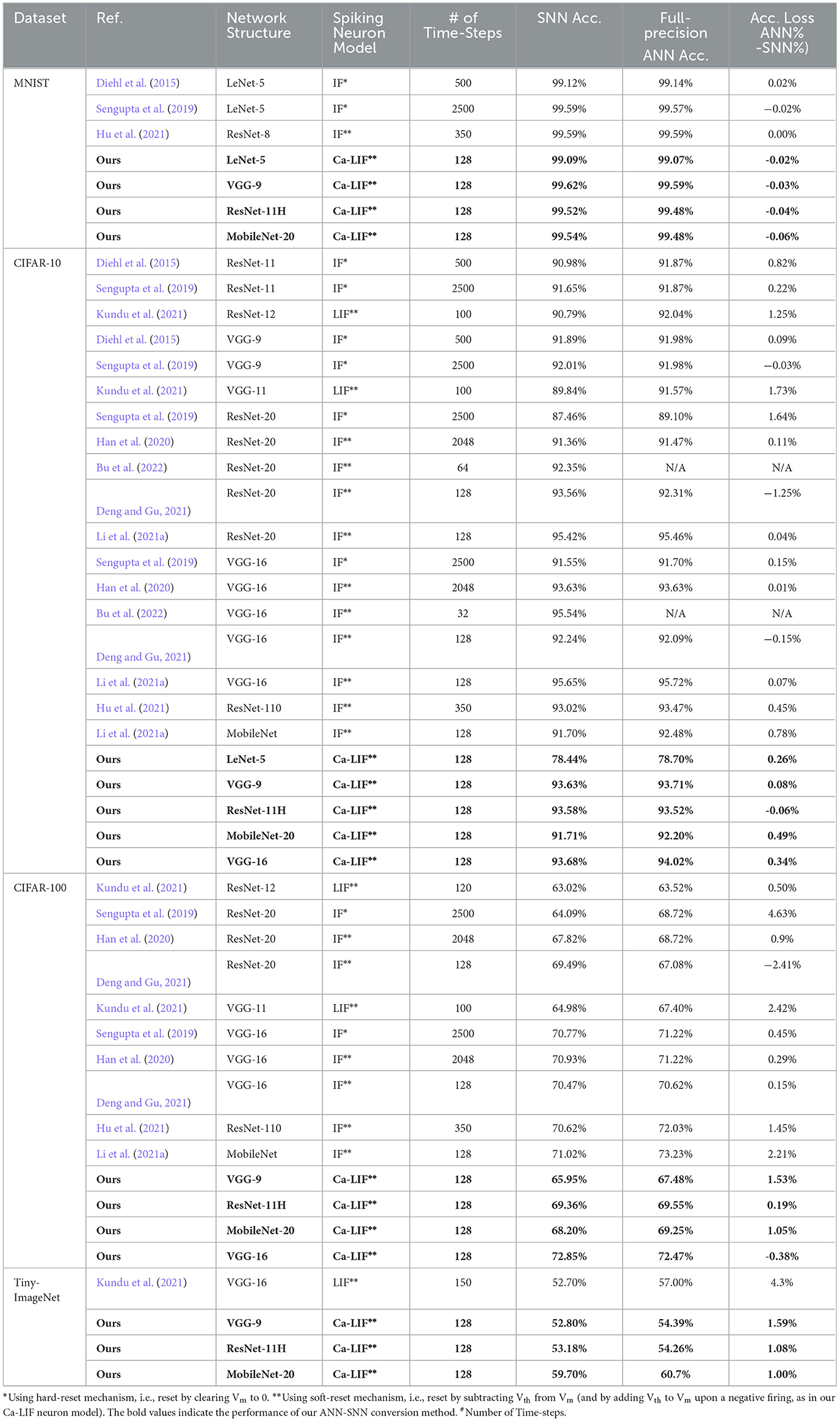
Table 2. Accuracy comparison between our and other ANN-to-SNN conversion methods.
For the MNIST dataset, the accuracies of our SNNs are a little higher than full-precision ANNs due to the higher accuracies of the QAT-trained ANNs. When it comes to CIFAR-10, the accuracy of our VGG-9 (93.63% for T = 128) surpasses those provided by Diehl et al. (2015), Sengupta et al. (2019), and Kundu et al. (2021). Using fewer time steps, our ResNet-11H on CIFAR-10 (93.58% for T =128) exceeds those using the same structure provided by Diehl et al. (2015) and Sengupta et al. (2019) and the deeper ResNet structure provided by Sengupta et al. (2019), Han et al. (2020), Hu et al. (2021), and Deng and Gu (2021). As compared to Bu et al. (2022) (92.35% for T = 64), our ResNet-11H (93.44% for T = 64) also has a better performance. The reason that the accuracy of our ResNet-11H is lower than that of Deng et al. (2022) will be discussed in section 4.4. The accuracy of our MobileNet-20 is slightly superior to that of Li et al. (2021a), while our VGG-16 on CIFAR-10 is preferable to Sengupta et al. (2019) and Han et al. (2020) in terms of both accuracy and latency (i.e., number of time steps). The accuracy of our VGG-16 is a little lower than that provided by Bu et al. (2022) and Li et al. (2021a) due to their high-accuracy baseline full-precision ANN, while our method relies on the QAT framework which produces a less-accurate ANN model for conversion. Fortunately, our method requires no complex operations like modifying the loss function mentioned by Bu et al. (2022) or post-processing calibrations mentioned by Li et al. (2021a). For the CIFAR-100 dataset, our ResNet-11H SNN also transcends more complex ResNet structures (Sengupta et al., 2019; Han et al., 2020; Hu et al., 2021) while falling behind (Deng and Gu, 2021). The accuracy and the latency metrics of our VGG-16 on CIFAR-100 outperform those using the same network architecture (Sengupta et al., 2019; Han et al., 2020; Deng and Gu, 2021).
Regarding the Tiny-Image-Net dataset, the overall performance (accuracy, latency, and ANN-to-SNN accuracy loss) of all our networks defeat those of Kundu et al. (2021).
In general, Table 2 indicates that our SNNs converted from QAT-trained ANNs can achieve competitively high recognition accuracies across all the used network structures on the benchmark image datasets, when compared to the similar network topologies used in other studies. Our SNN accuracy loss with respect to the corresponding full-precision ANNs also keeps as low as that of other studies. Moreover, in our study, the low-precision data quantization in ANNs allows an intermediate temporal window of T = 128 time steps for the converted SNNs to complete inference at an acceptable computational overhead on potential neuromorphic hardware platforms.
Table 3 Further uses the VGG-16 structure and CIFAR-10 dataset to test the accuracies of our converted SNNs with varying time steps and compares them with some recent ANN-to-SNN conversion researches. Our study surpasses Han et al. (2020), Han and Roy (2020) and Ding et al. (2021) totally under all time-step configurations. Our SNN accuracy is still comparably competent when using a relatively short time length of T = 32 time steps. However, when the time window is as extremely short as T = 16 or 8, our SNN accuracies start to obviously lag the ones obtained by Deng and Gu (2021), Bu et al. (2022), and Li et al. (2022b). Similar conclusions can be drawn from Table 4, where our study is compared with other studies on the SNN accuracies on the more challenging CIFAR-100 dataset. Our SNN accuracies are comparable to the others when T is 32 time steps or longer, but obviously lower for T = 8 and 16 time steps. We deem this accuracy degradation as the cost of adopting an off-the-shelf QAT ANN training toolkit without dedicated optimizations toward low-latency inference as employed in Deng and Gu (2021), Bu et al. (2022), and Li et al. (2022b). The recently emerged direct SNN training methods can also reach a relatively high accuracy while consuming much fewer time steps < 10 (Guo et al., 2021, 2022a,b,c,d; Deng et al., 2022; Kim et al., 2022; Li et al., 2022a). However, evaluating direct SNN training methods is out of the scope of this article.
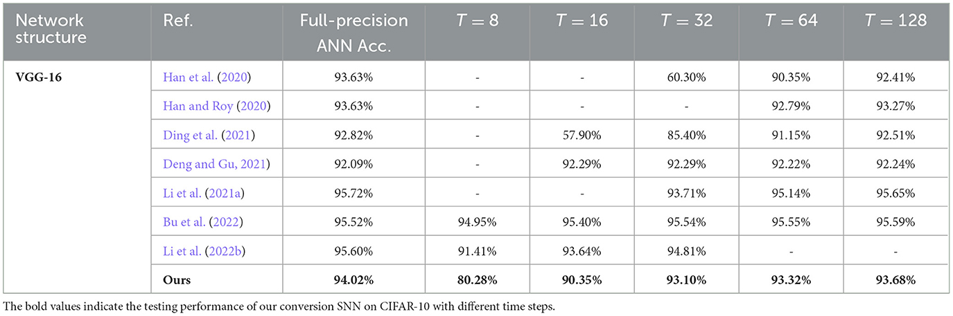
Table 3. Testing accuracies of the SNNs on CIFAR-10 with different time steps.
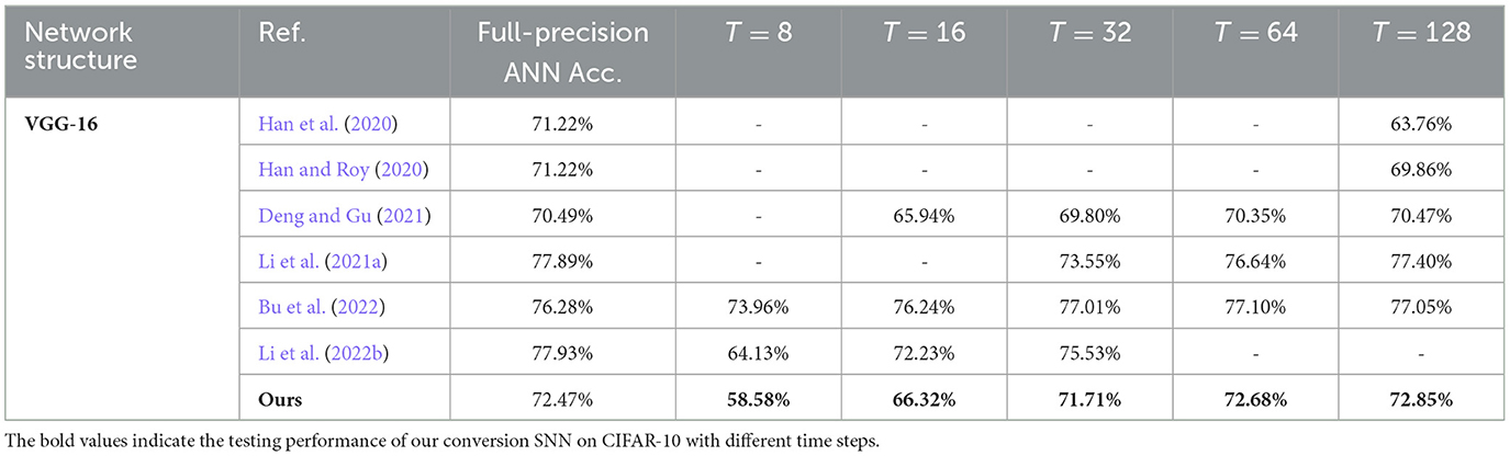
Table 4. Testing accuracies of the SNNs on CIFAR-100 with different time steps.
The concept of a negative spike has also been proposed by Kim et al. (2020). However, this work differs from theirs mainly in two aspects. First, the neuron model by Kim et al. (2020) has no membrane potential leakage. Rather, it adopts an extra constant input current to represent the bias term in the ANN ReLU. By contrast, our Ca-LIF model naturally incorporates the bias term in the more bio-plausible leakage term. Second and more importantly, the purposes of firing negative spikes are different. The negative spike mentioned by Kim et al. (2020) is only for modeling the negative part of the leaky-ReLU unit widely required in object detection, while our Ca-LIF neuron uses negative spikes to counter-balance the early emitted positive spikes so that when the net input zs in Equation (3b) aggregated over the entire time window T is negative, the final signed spike count can be zero, which thus closely emulates the quantized ReLU function in classification tasks, as explained in Section 3.1 and 3.2. Some previous ANN-to-SNN works do not adopt such methods but employed more complex threshold/weight balancing operations required to compensate for the early emitted positive spikes (Diehl et al., 2015; Rueckauer et al., 2017; Han et al., 2020; Ho and Chang, 2021; Liu et al., 2022). In this regard, although judging the sign of the spikes puts forward marginally additional computational overhead, it considerably eliminates the tedious post-conversion steps like threshold/weight balancing.
One limitation of the proposed QAT ANN-to-SNN conversion framework, as well as other ANN-to-SNN conversion methods, is that the input spike coding can only employ a rate-coding paradigm, where input spike frequency or count is proportional to the pixel intensity to be encoded. This requires multiple to dozens of spikes for each pixel. These ANN-to-SNN conversion methods cannot accommodate the more computationally efficient temporal coding scheme (Mostafa, 2018), where each pixel is encoded into only one spike whose precise emission time is conversely proportional to the pixel intensity, and each neuron in the SNN is only allowed to fire at most once in response to an input sample. However, as mentioned earlier, since our method can adapt to any available QAT training toolkit, we can resort to those supporting binary or ternary activations, so that the total spikes propagated through our converted SNNs would be largely reduced, with the required inference time window length considerably shortened. Therefore, the gap between the computational overheads of our converted SNNs and the one mentioned by Mostafa (2018) using temporal coding can be well bridged.
5. Conclusion
This study proposes a ReLU-equivalent Ca-LIF spiking neuron model and a QAT-based ANN-to-SNN conversion framework requiring no post-conversion operations, to achieve comparably high SNN accuracy in object recognition tasks with an intermediately short temporal window ranging from 32 to 128 time steps. We employed an off-the-shelf PyTorch QAT toolkit to train quantized deep ANNs and directly exported the learned weights to SNNs for inference without post-conversion operations. Experimental results demonstrated our converted SNNs of typical deep network structures can obtain competitive accuracies on various image datasets compared to previous studies while requiring a reasonable number of time steps for the inference. The proposed approach might also be applied to deploy deeper SNN architectures such as MobileNetv2 and VGG-34. Our future research will also include hardware implementation for SNN inference based on our Ca-LIF neurons.
Data availability statement
Publicly available datasets were analyzed in this study. The MNIST dataset is available at http://yann.lecun.com/exdb/mnist/. The CIFAR-10 and CIFAR-100 is accessible at https://www.cs.toronto.edu/~kriz/cifar.html. The Caltech-101 dataset and the Tiny-ImageNet can be found at https://www.kaggle.com/c/tiny-imagenet.
Author contributions
HG conceptualized the problem, implemented the algorithm, performed the experiments, and wrote the original manuscript. CS conceptualized the problem, supervised the work, funded the project, and revised the manuscript. MT revised the manuscript and supervised the work. JH, HW, and TW guided the implementation and tested the algorithms. ZZ collected the datasets. JY and YW revised the manuscript. All authors contributed to the article and approved the submitted version.
Funding
This study was funded in part by the National Key Research and Development Program of China (Grant No. 2019YFB2204303), in part by the National Natural Science Foundation of China (Grant No. U20A20205), in part by the Key Project of Chongqing Science and Technology Foundation (Grant Nos. cstc2019jcyj-zdxmX0017 and cstc2021ycjh-bgzxm0031), in part by the Pilot Research Project (Grant No. H20201100) from Chongqing Xianfeng Electronic Institute Co., Ltd., in part by the Open Research Funding from the State Key Laboratory of Computer Architecture, ICT, CAS (Grant No. CARCH201908), in part by the innovation funding from the Chongqing Social Security Bureau and Human Resources Dept. (Grant No. cx2020018), and in part by the Chongqing Science and Technology Foundation (Postdoctoral Foundation) (Grant No. cstc2021jcyj-bsh0126).
Acknowledgments
We thank Jing Yang for guidance and the reviewers for their valuable contributions.
Conflict of interest
The authors declare that the research was conducted in the absence of any commercial or financial relationships that could be construed as a potential conflict of interest.
Publisher's note
All claims expressed in this article are solely those of the authors and do not necessarily represent those of their affiliated organizations, or those of the publisher, the editors and the reviewers. Any product that may be evaluated in this article, or claim that may be made by its manufacturer, is not guaranteed or endorsed by the publisher.
References
Brader, J. M., Senn, W., and Fusi, S. (2007). Learning real-world stimuli in a neural network with spike-driven synaptic dynamics. Neural Comput. 19, 2881–2912. doi: 10.1162/neco.2007.19.11.2881
Bu, T., Fang, W., Ding, J., Dai, P., Yu, Z., Huang, T., et al. (2022). “Optimal ANN-SNN conversion for high-accuracy and ultra-low-latency spiking neural networks,” in International Conference on Learning Representations (ICLR).
Deng, S., and Gu, S. (2021). “Optimal conversion of conventional artificial neural networks to spiking neural networks,” International Conference on Learning Representations (ICLR) (Vienna, Austria).
Deng, S., Li, Y., Zhang, S., and Gu, S. (2022). “Temporal efficient training of spiking neural network via gradient re-weighting,” in International Conference on Learning Representations (ICLR).
Diehl, P. U., Neil, D., Binas, J., Cook, M., Liu, S.-.C, Pfeiffer, M., et al. (2015). “Fast-classifying, high accuracy spiking deep networks through weight and threshold balancing,” in 2015 Internation al Joint Conference on Neural Networks (IJCNN) (Killarney: IEEE), 1–8.
Ding, J., Yu, Z., Tian, Y., and Huang, T. (2021). “Optimal ANN-SNN conversion for fast and accurate inference in deep spiking neural networks,” in Proceedings of the Thirtieth International Joint Conference on Artificial Intelligence.
Dubhir, T., Mishra, M., and Singhal, R. (2021). “Benchmarking of quantization libraries in popular frameworks,” 9th IEEE International Conference on Big Data (IEEE BigData) (New York, NY: IEEE), 3050–3055.
Guo, W. Z., Fouda, M. E., Eltawil, A. M., and Salama, K. N. (2021). Neural coding in spiking neural networks: a comparative study for robust neuromorphic systems. Front. Neurosci. 15, 21. doi: 10.3389/fnins.2021.638474
Guo, Y., Chen, Y., Zhang, L., Liu, X., Wang, Y., Huang, X., et al. (2022a). IM-loss: information maximization loss for spiking neural networks. Adv Neural Inf Processing Syst. 11, 36–52. doi: 10.1007/978-3-031-20083-0_3
Guo, Y., Chen, Y., Zhang, L., Wang, Y., Liu, X., Tong, X., et al. (2022b). “Reducing information loss for spiking neural networks,” in Computer Vision–ECCV 2022, 17th. European Conference (Tel Aviv: Springer), Part XI, 36–52.
Guo, Y., Tong, X., Chen, Y., Zhang, L., Liu, X., Ma, Z., et al. (2022c). “RecDis-SNN: rectifying membrane potential distribution for directly training spiking neural networks,” in Proceedings of the IEEE/CVF Conference on Computer Vision and Pattern Recognition (CVPR), 326–335. doi: 10.1109/CVPR52688.2022.00042
Guo, Y., Zhang, L., Chen, Y., Tong, X., Liu, X., Wang, Y., et al. (2022d). “Real spike: Learning real-valued spikes for spiking neural networks,” in Computer Vision–ECCV 2022, 17th. European Conference (Tel Aviv, Israel), Part XII, 52–68.
Han, B., and Roy, K. (2020). “Deep spiking neural network: energy efficiency through time based coding,” 16th European Conference on Computer Vision (ECCV) (Glasgow: Springer), 388–404.
Han, B., Srinivasan, G., and Roy, K. (2020). “RMP-SNN: residual membrane potential neuron for enabling deeper high-accuracy and low-latency spiking neural network,” in 2020 IEEE/CVF Conference on Computer Vision and Pattern Recognition (CVPR) (Seattle, WA: IEEE), 13555–13564. doi: 10.1109/CVPR42600.2020.01357
Ho, N. D., and Chang, I. J. (2021). “TCL: an ANN-to-SNN Conversion with Trainable Clipping Layers,” 2021 58th ACM/IEEE Design Automation Conference (DAC) (San Francisco, CA: IEEE).
Howard, A. G., Zhu, M., Chen, B., Kalenichenko, D., Wang, W., Weyand, T., et al. (2017). Mobilenets: Efficient convolutional neural networks for mobile vision applications. arXiv preprint arXiv:1704.04861. doi: 10.48550/arXiv.1704.04861
Hu, Y., Tang, H., and Pan, G. (2021). “Spiking deep residual networks,” IEEE Transactions on Neural Networks and Learning Systems (IEEE), 1—6. doi: 10.1109/tnnls.2021.3119238
Hunsberger, E., and Eliasmith, C. (2016). Training spiking deep networks for neuromorphic hardware. arXiv preprint arXiv:1611.05141. doi: 10.13140/RG.2.2.10967.06566
Ioffe, S., and Szegedy, C. (2015). Batch normalization: accelerating deep network training by reducing internal covariate shift. Int. Conf Machine Learn. 1, 448–456. doi: 10.5555/3045118.3045167
Kim, S., Park, S., Na, B., and Yoon, S. (2020). Spiking-YOLO: spiking neural network for energy-efficient object detection. Proc. AAAI Conf. Arti. Int. 34, 11270–11277. doi: 10.1609/aaai.v34i07.6787
Kim, Y., Li, Y., Park, H., Venkatesha, Y., and Panda, P. (2022). “Neural architecture search for spiking neural networks,” in 17th European Conference on Computer Visio (ECCV) Cham: Springer Nature Switzerland.
Kundu, S., Datta, G., Pedram, M., and Beerel, P. A. (2021). “Spike-thrift: towards energy-efficient deep spiking neural networks by limiting spiking activity via attention-guided compression,” in 2021 IEEE Winter Conference on Applications of Computer Vision (WACV) (IEEE).
LeCun, Y., Bengio, Y., and Hinton, G. (2015). Deep learning. Nature 521, 436–444. doi: 10.1038/nature14539
Lecun, Y., Bottou, L., Bengio, Y., and Haffner, P. (1998). Gradient-based learning applied to document recognition. Proc. IEEE 86, 2278–2324. doi: 10.1109/5.726791
Lee, C., Sarwar, S., Panda, P., Srinivasan, G., and Roy, K. (2020). Enabling spike-based backpropagation for training deep neural network architectures. Front. Neurosci. 14, 119. doi: 10.3389/fnins.2020.00119
Li, Y., Deng, S., Dong, X., Gong, R., and Gu, S. (2021a). “A free lunch from ann: towards efficient, accurate spiking neural networks calibration,” in International Conference on Machine Learning (ICML) 6316–6325.
Li, Y., Deng, S., Dong, X., and Gu, S. (2022b). Converting artificial neural networks to spiking neural networks via parameter calibration. arXiv preprint arXiv:2205.10121. doi: 10.48550/arXiv.2205.10121
Li, Y., Guo, Y., Zhang, S., Deng, S., Hai, Y., Gu, S., et al. (2021b). Differentiable spike: Rethinking gradient-descent for training spiking neural networks. Adv. Neural Inf. Proc. Syst. 34, 23426–23439.
Li, Y., Zhao, D., and Zeng, Y. (2022a). BSNN: Towards faster and better conversion of artificial neural networks to spiking neural networks with bistable neurons. Front. Neurosci. 16:991851. doi: 10.3389/fnins.2022.991851
Liu, F., Zhao, W., Chen, Y., Wang, Z., and Jiang, L. (2022). Spikeconverter: an efficient conversion framework zipping the gap between artificial neural networks and spiking neural networks. Proc AAAI Conf Artif Int. 36, 1692–1701. doi: 10.1609/aaai.v36i2.20061
Mostafa, H. (2018). Supervised learning based on temporal coding in spiking neural networks. IEEE Trans Neural Networks Learn. Syst. 29, 7, 3227–3235. doi: 10.1109/TNNLS.2017.2726060
PyTorch Foundation (2022). E. coli. Available online at: https://pytorch.org/docs/stable/quantizatio-n.html#module-torch.quantization (accessed November 18, 2022).
Roy, K., Jaiswal, A., and Panda, P. (2019). Towards spike-based machine intelligence with neuromorphic computing. Nature 575, 607–617. doi: 10.1038/s41586-019-1677-2
Rueckauer, B., Lungu, I. A., Hu, Y., Pfeiffer, M., and Liu, S. C. (2017). Conversion of continuous-valued deep networks to efficient event-driven networks for image classification. Front. Neurosci. 11, 682. doi: 10.3389/fnins.2017.00682
Sengupta, A., Ye, Y., Wang, R., Liu, C., and Roy, K. (2019). Going deeper in spiking neural networks: VGG and residual architectures. Front. Neurosci. 13, 95. doi: 10.3389/fnins.2019.00095
Yang, X., Zhang, Z. X., Zhu, W. P., Yu, S. M., and Liu, L. Y. (2020). Deterministic conversion rule for CNNs to efficient spiking convolutional neural networks. Sci. China Inf. Sci. 63:1–19. doi: 10.1007/s11432-019-1468-0
Keywords: neuromorphic computing, spiking neural network, ANN-to-SNN conversion, deep SNNs, quantization-aware training
Citation: Gao H, He J, Wang H, Wang T, Zhong Z, Yu J, Wang Y, Tian M and Shi C (2023) High-accuracy deep ANN-to-SNN conversion using quantization-aware training framework and calcium-gated bipolar leaky integrate and fire neuron. Front. Neurosci. 17:1141701. doi: 10.3389/fnins.2023.1141701
Received: 10 January 2023; Accepted: 07 February 2023;
Published: 08 March 2023.
Edited by:
Yufei Guo, China Aerospace Science and Industry Corporation, ChinaReviewed by:
Yuhang Li, Yale University, United StatesFeichi Zhou, Southern University of Science and Technology, China
Copyright © 2023 Gao, He, Wang, Wang, Zhong, Yu, Wang, Tian and Shi. This is an open-access article distributed under the terms of the Creative Commons Attribution License (CC BY). The use, distribution or reproduction in other forums is permitted, provided the original author(s) and the copyright owner(s) are credited and that the original publication in this journal is cited, in accordance with accepted academic practice. No use, distribution or reproduction is permitted which does not comply with these terms.
*Correspondence: Cong Shi, shicong@cqu.edu.cn