A general and efficient method for incorporating precise spike times in globally time-driven simulations
- 1 Functional Neural Circuits Group, Faculty of Biology, Albert-Ludwig University of Freiburg, Freiburg im Breisgau, Germany
- 2 Bernstein Center Freiburg, Albert-Ludwig University of Freiburg, Freiburg im Breisgau, Germany
- 3 RIKEN Brain Science Institute, Wako, Japan
- 4 RIKEN Computational Science Research Program, Wako, Japan
Traditionally, event-driven simulations have been limited to the very restricted class of neuronal models for which the timing of future spikes can be expressed in closed form. Recently, the class of models that is amenable to event-driven simulation has been extended by the development of techniques to accurately calculate firing times for some integrate-and-fire neuron models that do not enable the prediction of future spikes in closed form. The motivation of this development is the general perception that time-driven simulations are imprecise. Here, we demonstrate that a globally time-driven scheme can calculate firing times that cannot be discriminated from those calculated by an event-driven implementation of the same model; moreover, the time-driven scheme incurs lower computational costs. The key insight is that time-driven methods are based on identifying a threshold crossing in the recent past, which can be implemented by a much simpler algorithm than the techniques for predicting future threshold crossings that are necessary for event-driven approaches. As run time is dominated by the cost of the operations performed at each incoming spike, which includes spike prediction in the case of event-driven simulation and retrospective detection in the case of time-driven simulation, the simple time-driven algorithm outperforms the event-driven approaches. Additionally, our method is generally applicable to all commonly used integrate-and-fire neuronal models; we show that a non-linear model employing a standard adaptive solver can reproduce a reference spike train with a high degree of precision.
1 Introduction
Discrete-time neuronal network simulation strategies typically constrain spike times to a grid determined by the computational step size. For many scientific questions this does not seem to present a problem, as long as the computational step size is chosen sufficiently small. However, in a worst case scenario, this can have the effect of introducing artificial network synchrony (Hansel et al., 1998). Moreover, it is difficult to make theoretical predictions about the required degree of spike time accuracy for a given scientific question. For these reasons, it is necessary to have efficient techniques available to calculate spike times in continuous time.
There are at least two approaches that can be employed to achieve this. One approach is to incorporate additional techniques to handle off-grid spikes in a globally time-driven algorithm (Hansel et al., 1998; Shelley and Tao, 2001). Morrison et al. (2007) presented a general method of handling off-grid spiking in combination with exact subthreshold integration of integrate-and-fire neuronal models in discrete time-driven simulations. The general principle is to process incoming spikes sequentially within a time step. The dynamics is propagated from spike to spike and then to the end of the time step. If any of these propagation steps results in a superthreshold value for the membrane potential, then an outgoing spike is calculated by interpolation. For the purposes of this work we will refer to a global simulation algorithm as “time-driven” if the state of each neuron in turn is updated on an equally spaced time grid. We will refer to an implementation of a neuron model as being “time-driven” if its state is updated on the grid defined by the simulation algorithm (potentially also at intermediate points), and spikes are detected by comparison of the neuronal state before and after an update.
An alternative approach is to use a globally event-driven algorithm. A prerequisite for this approach is that a neuron model can predict when it will next spike. Unfortunately, most popular integrate-and-fire models do not have invertible dynamics, and so the next spike time cannot be expressed in closed form. This state of affairs has encouraged the development of elegant spike prediction methods for specific neuron models. Brette (2007) addresses the problem of spike prediction for the linear leaky integrate-and-fire neuron with exponentially decaying post-synaptic currents (PSCs) by converting the dynamics of the membrane potential into a polynomial equation, and finding the largest root. Common numerical means like Descartes’ rule and Sturm’s theorem are applicable. The solution of D’Haene et al. (2009) is to generate an invertible function which acts as an upper limit for the membrane potential excursion. If the upper limit exhibits a threshold crossing, a modified Newton–Raphson technique is applied to localize the spike in the relevant interval. A similar scheme was independently proposed by van Elburg and van Ooyen (2009). In the following, we will refer to a global simulation algorithm as “event-driven” if it maintains a central queue of events and only updates neurons when they receive an event. We consider an implementation of a neuronal model to be “event-driven” if it is capable of predicting its next spike time (if any) on receiving an event.
A third approach is taken by Zheng et al. (2009). They abandon time as the stepping variable and present a technique to discretize the voltage state space. As fewer integration steps are needed when the membrane potential does not exhibit large fluctuations, they show that their voltage-stepping technique can result in better efficiency than time-stepping methods. A thorough analysis of this approach lies outside the scope of the current manuscript; in the following we restrict our investigations to time-driven and event-driven techniques.
In this paper, we present a generalized and improved version of one of the techniques presented in Morrison et al. (2007): in the case of linear model dynamics, the neuron state is propagated between spikes using Exact Integration (Rotter and Diesmann, 1999) and iterative techniques are used to locate outgoing spikes. Unlike the previous study, the accuracy of the spike time calculation does not depend on the computation step size. In the case of non-linear model dynamics, the state integration is carried out by a standard numerical solver.
In order to compare the performance of our approach with event-driven implementations of the same model, we develop a method of embedding event-driven neuron model implementations in the globally time-driven framework provided by NEST (Gewaltig and Diesmann, 2007; Eppler et al., 2009). We can therefore implement the same neuronal model using our technique, the technique presented in Brette (2007) and a technique based on the idea described in D’Haene et al. (2009) and compare their accuracy and run time costs, and thus their efficiency. This analysis does not disadvantage the event-driven techniques, for the following reasons. First, both time-driven and event-driven algorithms have complexity which is linear with respect to the number of neurons, but the multiplicative factor is typically higher for event-driven simulations, particularly in the regime of realistic connectivity and spike rates considered here (for complexity analysis, see Brette et al., 2007). Thus embedding event-driven implementations in a globally time-driven framework should not result in a poorer run time performance than in an event-driven framework. Second, we have taken great care to embed the implementations in such a way that they benefit from the advantages of the time-driven framework (e.g., greater cache efficiency through local buffering of imminent incoming events) without suffering any of the disadvantages (e.g., no additional state updates dependent on the computation step size). This is described in greater detail in Section 2.2.2.
All the implementations of the specific neuron model investigated use an iterative search technique to locate the threshold crossing, for which the target precision must be specified (Section 2.3.1). This value cannot be chosen arbitrarily small, as only a limited number of significant digits are available in the double representation of floating point numbers used in our simulations (Press et al., 1992). The finest target precision that can be required without causing the search algorithm to enter an infinite loop yields 14 reliable decimal places for the determination of the membrane potential (in mV). This is two orders of magnitude greater than the machine epsilon ϵ, the smallest number such that 1 + ϵ can be distinguished from 1 in double representation. Similarly, in our previous study, we discovered that when spike times are expressed as fractional and integer components expressing, respectively, the offset in milliseconds to the right border of a 1ms time interval, their differences achieve a maximum of 13 reliable decimal places (Morrison et al., 2007). This is due to the two to three decimal places that are lost from the theoretical maximum in calculating the neuronal dynamics as a result of the repeated floating point operations involved (Press et al., 1992). Therefore, in the absence of an analytical solution, if an implementation produces spike times that cannot be distinguished from the spike times generated by an appropriate reference implementation in the first 13 decimal places, we refer to this implementation as being accurate up to the non-discrimination accuracy. As a corollary, we can compare absolute spike times less than 1 s in units of milliseconds using double representation without loss of accuracy.
Whereas the accuracy of an implementation can be easily determined by comparing the spike trains it generates in a single neuron simulation to that of a reference implementation, to determine the computational costs of an implementation it is more useful to measure the simulation time of a reasonably sized network. Single neuron simulations may not give a reliable measure of computation costs, as the entire data will fit into a computer’s cache memory, causing differences in the demands on memory bandwidth to be overlooked. However, recurrent networks typically exhibit chaotic dynamics, such that the slightest difference will lead to completely different spike trains in a short time, irrespective of whether time-driven or event-driven methods are used. Therefore, no measurement of accuracy can be defined for such systems. To overcome this problem, we treat a recurrent network simulation as a stand-in for a model in which a high degree of accuracy would be both meaningful and desirable. As in our earlier study (Morrison et al., 2007), we consider the simulation time of a recurrent network as a function of the accuracy measured in a single neuron simulation with the same input statistics. The efficiency of a given implementation is then defined as the run time cost to achieve a particular accuracy goal.
When no spikes are missed, our time-driven implementation of the linear model is accurate up to the non-discrimination accuracy for a lower computational cost than the event-driven implementations. This holds even if the neuronal parameters are chosen in a biologically unrealistic fashion in order to provide a best-case scenario for an event-driven implementation and the time step is chosen to be very large (e.g., 1 ms). We investigate the probability of missing a spike for a wide range of input and output rates and quantitatively identify operating regimes in which event-driven algorithms could potentially exhibit better performance than time-driven algorithms. We further show that, unlike the event-driven approaches, which are tailored to a specific neuronal model, our technique is generally applicable to all integrate-and-fire point-neuron models, including non-linear models.
The conceptual and algorithmic work described here is a module in our long-term collaborative project to provide the technology for neural systems simulations (Gewaltig and Diesmann, 2007). Preliminary results have been published in abstract form (Diesmann et al., 2008; Hanuschkin et al., 2008; Kunkel et al., 2009).
2 Materials and Methods
2.1 Example Neuron Models
In order to compare like with like, the main part of our work focuses on the leaky integrate-and-fire model with exponentially decaying PSCs that can be implemented by all three of the methods considered here: the event-based techniques of Brette (2007) and D’Haene et al. (2009) and the time-driven technique based on Morrison et al. (2007). We restrict the linear subthreshold dynamics to a single synaptic time constant to obtain a benchmark model that is favorable for the event-driven strategies. The details of this model are given in Section 2.1.1. To demonstrate the generality of our technique, we also apply it to the non-linear adaptive exponential integrate-and-fire neuron model described in Section 2.1.2.
2.1.1 Neuron model with linear subthreshold dynamics
The subthreshold membrane potential dynamics follows the equation

where Cm is the capacitance, τm the membrane time constant, Ix is an external direct current, Isyn is the synaptic input current and the resting potential is set to 0. The synaptic current follows
where  denotes the k-th spike of the incoming synapse j with synaptic amplitude
  , Isyn(0) is the initial value and H denotes the Heaviside step function.
The neuron model is characterized by the resting potential V0 = 0 mV, the membrane time constant τm = 10 ms, the capacitance Cm = 250 pF and the threshold Θ = 20 mV. When the membrane potential crosses the threshold a spike is emitted and the membrane potential is clamped to Vreset = V0 for the duration of the refractory period, τref = 2 ms. The synaptic time constant τ = 1 ms is identical for all synapses and results in a biologically realistic value of 2.6 ms for the rise time of the post-synaptic potential (PSP) starting from resting potential. The peak amplitudes of excitatory and inhibitory PSCs are set to  and
and  respectively. The solution to the differential equation (Eq. 1) describing the membrane potential trajectory of the model neuron is derived in the Appendix.
2.1.2 Neuron model with non-linear subthreshold dynamics
We choose the adaptive exponential integrate-and-fire neuron model (Brette and Gerstner, 2005; Gerstner and Brette, 2009), which is used as a standard model in the large-scale European research project FACETS (2009), to demonstrate the compatibility of our approach with non-linear neuron models. Following Naud et al. (2008), we refer to this as the AdEx model. The membrane potential V and the adaptation current w are described by the coupled ordinary differential equations (ODEs)

and
where gL is the leak conductance, EL the resting potential, ΔT a slope factor, Vth the threshold potential and τw the time constant of adaptation. When the membrane potential reaches Vpeak, it is reset to Vreset and the adaptation current is increased: w ← w + b. I describes the synaptic current and is expressed by

where Ee and Ei are the reversal potentials for excitation and inhibition. In our implementation a single input spike introduces a change in synaptic conductance modeled as an α-function:  , with x ∈ [e,i]. Jx is the peak amplitude of the conductance and is given by the synaptic weight. Hence, the synaptic conductances ge and gi fulfill
  . This second order linear time-invariant differential equation can be transformed into two coupled first order differential equations (for a review see Plesser and Diesmann, 2009). The whole set of first order differential equations is integrated with a fourth order Runge–Kutta–Fehlberg solver with adaptive step-size control based on the fifth order error estimate to ensure the target precision. Convenient routines are provided by the GNU Scientific Library (Galassi et al., 2006). The dynamics of the AdEx neuron is determined by the four bifurcation parameters a,b,τw and Vreset. We set these parameters such that tonic spiking is generated in response to constant input current, as described by Naud et al. (2008): a = 0.001 nS, b = 5 pA, τw = 5 ms, and Vreset = −70 mV. The scaling parameters are set to Cm = 250 pF, gL = 16 nS, EL = −70 mV, ΔT = 2 mV, Vth = −50 mV, and Vpeak = 0 mV. The synaptic input is characterized by the reversal potentials Ee = 0 mV, Ei = −80 mV and the time constants τe = τi = 1 ms.
2.2 Processing Continuous Spike Times in Globally Time-Driven Algorithms
To understand the similarities and differences between the time-driven and embedded event-driven methods, we first need to clarify the underlying globally time-driven scheduling algorithm. The simplest possible time-driven algorithm integrates the dynamics of each neuron in turn in time steps of h, sometimes also referred to as the computation step size or resolution. In this study, we use the simulator NEST (Gewaltig and Diesmann, 2007) which improves on this simple algorithm by introducing a communication interval, Tcomm = kh for k ≥ 1, which is the minimum interval in which spikes must be communicated to preserve causality. The communication interval is determined by the shortest synaptic delay in the network to be investigated (Morrison et al., 2005; Plesser et al., 2007; Morrison and Diesmann, 2008). Typically, the communication interval is substantially larger than the time step (e.g., 1 ms compared to 0.1 ms). Instead of visiting each neuron in turn in steps of h, the simulator visits each neuron in macro-steps of length Tcomm, each macro-step consisting of k micro-steps of length h. This is illustrated in Figures 1A,C for the case that k = 2. Note that all incoming spikes that are due to arrive at a neuron in a given communication interval are already queued locally at the neuron before the integration of that interval begins. After each neuron has been advanced by Tcomm, the network time is advanced and any spikes that were generated in the most recent interval are communicated. This reordering of update steps maximizes the number of operations performed sequentially on each neuron, which enhances cache efficiency and thus performance.
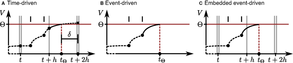
Figure 1. Propagation of the neuronal membrane potential V over time t according to different simulation strategies. Single vertical gray lines denote the borders of time steps of size h; double gray vertical lines indicate the communication intervals of size Tcomm. To simplify the illustrations, we let Tcomm = 2h. Vertical black bars indicate the arrival times of incoming spikes, and the horizontal red line shows the firing threshold Θ. Each filled circle denotes the final result of a neuronal dynamics calculation; a black cross indicates an intermediate result that is modified later. Dashed black curves indicate the trajectory of the membrane potential between calculation points to assist visualization. (A) Time-driven implementation (Section 2.2.1). The neuron advances in steps of h, while spikes are communicated after every communication interval, here 2h. All incoming spikes for the current interval Tcomm are buffered at the neuron before the start of the interval. The neuron integrates its dynamics from each incoming spike to the next and to the end of every time step. At the end of each update, a retrospective detection of threshold crossings in the preceding subinterval is performed. If the membrane potential is superthreshold at the right interval border, here indicated by the black cross at time t + 2h, an outgoing spike occurred within the interval. The spike time tΘ can be determined using interpolation techniques based on the neuronal state at the left and right interval states, or using an iterative technique (illustrated as a solid black curve) starting from the left border. The offset of the spike with respect to the next time step boundary is indicated by δ. The neuron state at the right interval border is then re-calculated by integrating its dynamics assuming a state reset at tΘ. (B) Event-driven implementation. The neuron state is updated every time the global event queue delivers a spike to it. Each time an incoming spike has been processed, a prediction strategy is applied in order to check for future threshold crossings. If an outgoing spike is predicted, an iterative technique is applied (solid line) to locate the threshold crossing, where the most recent spike defines the left border of the search. The search converges at tΘ unless it is aborted due to the arrival of another input spike. (C) Embedded event-driven implementation (Section 2.2.2). The simulation advances as described in (A), i.e., all incoming spikes for the next Tcomm interval are already buffered at the neuron. However, the neuronal state is updated according to those spikes as in (B), i.e., a threshold crossing prediction is performed for every incoming spike, followed by an iterative location technique (solid line) if necessary. No additional updates are performed at the end of each time step.
2.2.1 Time-driven implementations
The framework enabling continuous spike times to be processed in the globally time-driven simulator NEST (Gewaltig and Diesmann, 2007) has been previously described in great detail (Morrison et al., 2007). To summarize briefly, each spike is represented by an integer time stamp, which identifies the right border of the time step in which it was generated, as well as a floating point offset δ with double precision, which expresses the temporal difference between the calculated spike time and the integer time stamp. In Figure 1A, the time stamp of the generated spike is t + 2h and the offset is δ = t + 2h − tΘ. The sum of the time stamp and the synaptic delay gives the right border of the time step in which the spike becomes visible at the target neuron. Each time a neuron updates its dynamics by h, it processes all incoming spikes that become visible in that time step. In the case of linear dynamics, exact integration techniques (Rotter and Diesmann, 1999) can be applied; most non-linear neuron models require an efficient numerical solver.
The “canonical” implementation (Morrison et al., 2007) preserves the temporal order of the incoming spikes, and the neuron dynamics is propagated from one incoming spike to the next. Although this resembles an event-driven scheme on the level of the individual neurons (see Figure 1B), it differs in crucial ways. Firstly, spikes can be delivered to their targets immediately after generation; no global event queue is required and a neuron always has all the incoming spikes due to become visible in the next communication interval available in its local buffer before it begins to integrate its dynamics. Secondly, as the neuron state is updated at the end of each time step regardless of whether any spikes arrived in that period, no spike prediction algorithm is necessary. Instead, spike detection is performed retrospectively each time the neuronal state is updated, i.e., when processing a buffered incoming spike or at the end of a time step (see Figure 1A). In the case of the neuron models described in Section 2.1, the detection of a spike is simply checking the membrane potential at the right border of the most recently processed subinterval: if V(t) ≥ Θ, a spike occurs in that subinterval. It is possible to miss a spike if the membrane potential only has a brief superthreshold excursion and returns to subthreshold values before the end of the subinterval. However, given biologically realistic synaptic time constants and input rates, the time difference between the arrival of a spike and the maximum of the subsequent membrane potential excursion is usually greater than the typical length of a subinterval (i.e., the interspike interval of the incoming spike train) and so this case is rare. This issue is investigated in greater depth in Section 3.1.
Once a spike is detected, its location within the subinterval must be determined. In Morrison et al. (2007) the spike is located using interpolation. Since the values of both the membrane potential and its derivative are known at both borders of the subinterval, polynomials of order up to cubic can be fitted to the course of the membrane potential; the first root of the polynomial is used as an approximation for the spike time. The accuracy of the interpolation is dependent on the size of the interval and thus determined by the time step at fine resolutions and by the average interspike interval at coarse resolutions. In this manuscript we improve on the interpolation method by utilizing the iterative methods described in detail in Section 2.2.3 to progressively approximate the threshold crossing until a target precision is reached.
For the non-linear neuron model described in Section 2.1.2, it turns out that no iterative spike location is necessary due to the adaptive step size of the numerical solver. The neuron approaches the threshold so steeply that the step size chosen by the solver is much smaller than the interspike interval of the incoming spike train or the time step h. If the superthreshold condition is detected after an iteration of the solver, a linear interpolation is sufficient to localize the outgoing spike accurately.
The time-driven framework developed in Morrison et al. (2007) and improved here is applicable to any spiking neuron model for which a superthreshold condition can be detected and to any network in which spikes are subject to transmission delays; here we demonstrate its use in both the linear and non-linear neuron models described in Section 2.1.
2.2.2 Embedded event-driven implementations
To compare the performance of event-driven implementations (see Figure 1B) with that of time-driven implementations we construct a method of embedding the event-driven implementations proposed by Brette (2007) and D’Haene et al. (2009) in a globally time-driven simulator. This is illustrated in Figure 1C. An embedded event-driven implementation functions very similarly to a purely event-driven implementation, but differs from it in one key feature. In a purely event-driven scheme, the neuron is visited by the scheduling algorithm every time the global event queue sends a spike to it. All calculations, including predicting the next spike time, take place at these times. In an embedded event-driven scheme, due to the synchronization in intervals of Tcomm, all spikes that are due to arrive at a neuron within the next Tcomm interval are already buffered at the neuron at the start of that interval and can thus be processed sequentially in one visit of the scheduling algorithm. The cost for this is that the model has to check at the end of each Tcomm interval whether the neuron can spike without further input. If so, the neuron additionally has to check whether the spike is before the end of the interval (in which case it must be located and sent out) or not (in which case it can be ignored until the next Tcomm interval).
This approach results in the algorithm described in pseudocode in Algorithm 1. In the case of an embedded event-driven implementation, the algorithm proceeds as follows. On the arrival of each incoming spike a check is performed whether a future output spike had previously been predicted, i.e., whether after the last incoming spike was integrated, the neuronal state was such that it could become superthreshold without further input (spike_predicted is true). If so, an iterative search is made for the threshold crossing in the interval defined by the previous (left border) and current (right border) update events. If the search is successful, an output spike is emitted with the time determined by the search algorithm. Regardless of whether a spike was predicted, the neuronal state is then propagated up to the current update event, the new incoming spike is integrated and the prediction algorithm is performed to determine whether the neuron can become superthreshold in the absence of further input. At the end of each communication interval Tcomm, the embedded implementation checks whether a spike has been predicted. If so, it performs a search using the previous incoming spike as the left border and the end of the communication interval as the right border; this is necessary to preserve causality in the network. However, if in this case no outgoing spike occurs between the final incoming spike of a communication interval and the end of the interval, the variables tpred and spred store the preliminary results of the Newton–Raphson search. These variables can be used to initialize the search at the first update event in the next communication interval. The spike prediction algorithms employed in the approaches proposed by Brette (2007) and D’Haene et al. (2009) are briefly summarized in Sections 2.2.2.1 and 2.2.2.2, respectively; the iterative spike location techniques are described in Section 2.2.3.
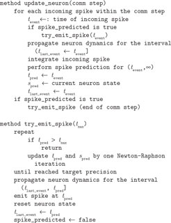
Algorithm 1. Algorithm to embed event-driven neuron model implementations into our time-driven simulator (Ggewaltig and Diesmann, 2007). The methods update_neuron_dynamics() and try_emit_spike() as well as the variables tlast_event, tpred, spred, and spike_predicted are members of the neuron model class. tlast_event is the time of the last update, tpred is the predicted time of the next outgoing spike, spred is the predicted state of the neuron at time tpred and spike_predicted is a Boolean variable indicating whether the neuron can fire without receiving additional excitatory input. Globally, the simulation advances in communication steps. Each neuron model instance is updated according to the currently processed communication step by calling its method update_neuron(comm step) once. Spike prediction is performed according to either the polynomial (Section 2.2.2.1) or the envelope (Section 2.2.2.2) method and results in the variable spike_predicted being set to true or false. This algorithm is based on the preconditions that the spike prediction strategy does not produce any false positives and that the Newton–Raphson technique converges at the first threshold crossing. For convenience pseudocode handling refractoriness is neglected. See also Figure 1.
Separating the spike prediction and spike location algorithms represents a deviation from a purely event-driven algorithm, in which a spike location algorithm is performed immediately after a positive spike prediction. However, deferring the location procedure until the next incoming event or end of a communication interval enhances the performance of the implementation. If the new incoming spike would arrive before the predicted outgoing spike, an iterative search using the previous spike as a left border and the new spike as a right border will fail much more rapidly than a full iterative search based solely on the left border will succeed, so the run time is reduced. If the new incoming spike would arrive after the predicted outgoing spike, then it costs no more to defer the actual search until later. We thus optimize for the common case that the next incoming spike will alter or cancel a previously predicted spike time. The cost of this optimization is an additional call to the try_emit_spike routine in the comparatively rare case that the neuronal state at the last incoming spike in a communication interval predicts a spike that lies beyond the border of that interval. Note that the use of the intermediate variables tpred and spred ensures that no additional search steps are carried out; the sole cost is the additional function call. This optimization is only possible in the embedded context; in a purely event-driven simulation, either a full search (Brette, 2007) or at least a scheduling of preliminary search results (D’Haene et al., 2009) must be performed after every positive spike prediction in order to maintain causality. Note that no operations are performed at the end of each computational time step h and so the complexity of the algorithm is dependent only on Tcomm and not on h. To achieve maximum performance of the embedded event-driven implementations we have reduced the algorithm to the most simple case. If the preconditions of reliable spike prediction and Newton–Raphson convergence cannot be met for a given neuron model, it is simple to develop a more general and robust form of Algorithm 1 that ensures correct integration of the model.
Embedding an event-driven neuron model implementation into a globally time-driven scheduling algorithm should result in an equal or better performance than a purely event-driven scenario under most circumstances. As discussed in Brette et al. (2007), the complexity of both time-driven and event-driven global scheduling algorithms is linear with respect to the number of neurons. However, a higher multiplicative factor is expected for event-driven simulations, particularly in the regime of realistic connectivity and spike rates leading to a total input rate in the order of 10 kHz. Moreover, a lower multiplicative factor is expected for the scheduling algorithm employed by NEST (Gewaltig and Diesmann, 2007) than for the naive time-driven algorithm on which the complexity analysis is based, due to the introduction of the communication interval Tcomm as described above. All the incoming spikes for the next communication interval are already stored locally at the neuron before the interval is processed. This means that a neuron can integrate all those incoming spikes in one visit from the scheduling algorithm. This is more cache-efficient than visiting each neuron in turn in time steps of h, as is the case for a naive time-driven algorithm. Assuming the rate of incoming spikes is such that at least one spike per communication interval is expected (e.g., 1000 Hz for Tcomm = 1 ms), this approach is also more cache-efficient than visiting each neuron in the network in the order determined by the times of incoming spikes, as is the case for a globally event-driven algorithm. Finally, as no neuronal state updates are carried out at the end of each time step, the number of operations performed on the global time grid is reduced to the minimum, thus the algorithmic complexity of the embedded implementation depends only on the communication interval Tcomm and not on the time step h.
2.2.2.1 Polynomial algorithm. The technique of Brette (2007) can be applied to linear integrate-and-fire neuron models with exponential synaptic currents. For the benchmark model described in Section 2.1.1 with equal synaptic time constants for excitation and inhibition and where the membrane time constant is an integer multiple of the synaptic time constant, the technique of Brette (2007) can be applied as follows. Setting V(t) = Θ and applying the substitution term  , The solution to the membrane potential dynamics is transformed into the polynomial

See the Appendix for a derivation of the solution to the dynamics (Eq. 1) and the definition of the multiplicative factors Vm and Vsyn. For a complete treatment, see Brette (2007).
The roots of this polynomial correspond to the threshold crossings of the membrane potential and can be located using numerical methods. However, as solving the polynomial can be computationally expensive, especially for polynomials of higher order, it is advantageous to perform a quick spike test to determine whether it is possible that the neuron would fire without further input. The quick spike test is based on Descartes’ rule of signs. For the general case of the neuron model described in Section 2.1.1 with differing synaptic time constants, the quick spike test can only be usefully applied for the case that τe > τi, which is not a typical parameter choice. In the case of our simplified neuron model with equal synaptic time constants, the quick spike test reduces to examining whether Vm > 0 and Vsyn < 0 are both true. If not, the neuron cannot spike without further input. If true, a full spike test based on Sturm’s algorithm is carried out to determine whether a threshold crossing will occur. For the technical details, see Brette (2007). In the original formulation, if a threshold crossing is predicted, a bisectioning algorithm is applied to define an interval in which the faster Newton–Raphson technique can be applied to finding the largest root of the polynomial given in Eq. 2. For the chosen benchmark model, we optimize performance by leaving out the bisectioning algorithm; this is justified in Section 2.2.3. To enhance its performance further we “hardwire” the polynomial representation to the order determined by the chosen neuronal parameters.
2.2.2.2 Envelope algorithm. D’Haene et al. (2009) proposed an alternative technique to simulate linear integrate-and-fire neuron models with synaptic currents that can be expressed as sums of exponentials in an event-driven scheme. In D’Haene and Schrauwen (2010) they demonstrate that their method can easily be applied to the neuron model proposed in Mihalas and Niebur (2010), which can generate richer neuronal dynamics than most other linear models.
Here, we briefly summarize the technique as applied to our simplified neuron model. After each incoming spike is integrated, a prediction must be made as to whether the neuron can fire without further input. As for the polynomial algorithm described above, in the case of our simplified neuron model a quick spike test consists of examining whether Vm > 0 and Vsyn < 0 in Eq. 2 are both true. If so, a full spike prediction is performed. The full spike prediction is based on approximating the maximum value of a function that is equal to or greater than the membrane potential excursion. We refer to this overshooting function as the envelope function. If the approximated maximum is subthreshold, the neuron will not spike without further input. If it is superthreshold, it is not certain whether the neuron would spike without further input and a method to localize the potential spike is initiated. Spike location is performed by a Newton–Raphson technique, which is adapted in such a way that it converges at the first threshold crossing of the membrane potential. For the details of the generation of the envelope function and the adaptation of the Newton–Raphson technique, see D’Haene et al. (2009). As the spike location method is an iterative method, intermediate results can be scheduled as preliminary spikes in the event queue and refined if they reach the front of the event queue without being invalidated by further input.
In the case of the chosen linear benchmark model, which has only one synaptic time constant, the maximum of the membrane potential can be analytically determined as given in Eq. 5 and the conventional Newton–Raphson technique converges at the first threshold crossing. We therefore implement the envelope algorithm of D’Haene et al. (2009) such that the envelope function is identical to the membrane potential trajectory and employ only a conventional Newton–Raphson technique. This represents a best-case scenario for this algorithm for the purposes of performance testing, but naturally does not permit the full flexibility of the original formulation of the method, which includes optimizations to facilitate partial state updates and speed up the simulation when the neuron model has multiple synaptic time constants.
2.2.3 Iterative spike location techniques
The benchmark neuron model described in Section 2.1.1 with equal synaptic time constants for excitation and inhibition has the property that whenever sufficient excitatory input causes a threshold crossing, the membrane potential function is concave. Consequently, a Newton–Raphson search starting at the left border is guaranteed to locate the first threshold crossing in an interval (i.e., the point where the membrane potential becomes superthreshold) and not the second threshold crossing (i.e., where the membrane potential relaxes back into the subthreshold regime). This means that any additional algorithm to ensure convergence at the first threshold crossing at the cost of slowing down the spike location is unnecessary. To optimize the speed of the embedded event-driven implementations, we deviate from their original formulations as follows. In case of the polynomial algorithm (Brette, 2007), the supplementary bisectioning algorithm is left out (compare Section 2.2.2.1). Additionally, the Newton–Raphson technique is directly applied to the membrane potential function instead of to its polynomial representation. In the case of the envelope algorithm of D’Haene et al. (2009), the generated envelope function is identical to the trajectory of the membrane potential and so the adapted Newton–Raphson technique (see Section 2.2.2.2) reduces to its best-case, which is the conventional Newton–Raphson technique.
Unlike the embedded event-driven implementations, which must perform a search after every positive prediction of a spike even if further input invalidates the search, the time-driven implementation presented in Sec. 2.2.1 localizes a threshold crossing only if a spike has been retrospectively detected in the previous subinterval. Consequently, the contribution of the spike location algorithm to the total run time can be considered independently from the spike detection. As most neuron models do not ensure correct convergence of the Newton–Raphson technique, it is useful to gain insight into the performance of different spike location algorithms. Therefore, we use the time-driven implementation of the benchmark neuron model to investigate the effect on the total run time of the previously used interpolation method (Morrison et al., 2007) which generates a solution in constant time, the Newton–Raphson technique which converges quadratically to a predefined target precision and the bisectioning technique which converges linearly. The interpolation method as well as the bisectioning technique are applicable to virtually all neuron models.
2.3 Analysis of the Linear Model
2.3.1 Single neuron simulations
Each experiment consists of 40 trials of 500 ms each at a given time step h, where h is varied systematically in base 2 representation between 20 and 2−14 ms (1 ms and approximately 0.06 μs). In each trial the neuron receives a unique realization of an excitatory Poissonian spike train at rate 1000·νsn and an inhibitory Poissonian spike train at 252·νsn, corresponding to input from 1008 excitatory and 252 inhibitory neurons firing independently at νsn. Additionally, the neuron receives either a constant external direct current Ix of 499 pA to drive the membrane potential to just below the firing threshold and a unique excitatory Poissonian spike train at νext = 2.71 kHz, or no external current (Ix = 0) and νext = 18.17 kHz. The choice of a high input current is intended to create a “best-case” stimulation protocol for the embedded event-driven implementations in terms of computation time, as the costs to process each incoming spike are higher for an embedded event-driven implementation than for a time-driven implementation (Section 2.2). Unless otherwise stated, νsn = 10 Hz and all neuronal parameters are set as in Section 2.1.1. This results in an input firing rate of 15.31 kHz for Ix = 499 pA and 30.77 kHz for Ix = 0 pA. In both cases the mean input current is 403.48 pA and the mean membrane potential is 16.14 mV, resulting in an output firing rate of approximately 10 Hz.
The spike times of the neuron are recorded in each trial. The integration error for a particular time step h is given by the median error in spike timing over all trials with respect to a reference spike train. Since the spike times cannot be calculated analytically, the reference spike train is defined to be the output of the envelope method (Section 2.2.2.2) at the finest resolution, i.e., 2−14 ms. The precision target for the iterative techniques to locate the threshold crossing, and thus the spike time, is 10−14 mV: the smallest value that can be specified that does not cause the search algorithm to enter an infinite loop due to the unreliability of the remaining decimal places in the double representation of floating point numbers.
2.3.2 Network simulations
The network simulation is based on the balanced random network model of Brunel (2000). It consists of NE = 10,080 excitatory and NI = 2,520 inhibitory neurons; each neuron receives 1008 synaptic connections randomly chosen from the excitatory population, 252 connections randomly chosen from the inhibitory population and an additional excitatory Poissonian spike train at νext = 2.71 kHz; peak PSC amplitudes are chosen as in Section 2.3.1. All synaptic delays in the network are set to 1 ms. The network activity is approximately asynchronous irregular (Brunel, 2000) with an average firing rate of 10 Hz. Note that the input and output firing rates of each neuron in the network are the same as for the single neuron simulation with νsn = 10 Hz. The simulation time step h is varied between 20 and 2−14 ms; the run time cost for a particular time step h is defined as the average length of time over five trials taken to simulate the network for one biological second at that time step.
2.3.3 Performance gain
To determine the performance gain of one neuron model implementation over another with respect to input and output rates, the simulation set-ups described above are altered as follows. The rate of the external Poissonian stimulation of the single neuron simulation (Section 2.3.1) is reduced to νext = 1 kHz and the peak amplitude of the resultant PSCs is increased to 87.18 pA. The single neuron input rate νsn is systematically varied to give a total rate of incoming spikes between 5 and 65 kHz. For each input rate the peak amplitude of the excitatory PSCs is systematically varied; the peak amplitude of the inhibitory PSCs is varied in proportion with  Each choice of synaptic strength leads to a different output rate νout; by averaging over 10 trials an empirical mapping νout (νsn,
  e) is constructed. Note that by disentangling the input and output rates in a network simulation we can treat them as independent variables. This technique is equivalent to investigating a series of networks with varying self-consistent rates, but without requiring the laborious tuning of connection strengths entailed by the latter approach.
The rate of the external Poissonian stimulation of the network (Section 2.3.2) is similarly reduced to νext = 1 kHz and the peak amplitude of the resultant PSCs is increased to 87.18 pA. The inter-neuron spike communication mechanism is disabled; to replace the recurrent input each neuron receives an excitatory Poissonian spike train at 1008·νsn and an inhibitory Poissonian spike train at 252·νsn. The input rate νsn and the peak amplitudes of the excitatory and inhibitory PSCs are set corresponding to the configurations determined for the empirical mapping described above. We perform three trials for each configuration of νsn,  e, and νout and determine the average time T required to simulate one biological second. The performance gain of an implementation y with respect to a reference implementation x is thus given by 100 × (Tx − Ty)/Tx.
2.4 Analysis of the Non-Linear Model
The dynamics of the non-linear neuron model is integrated using a 4th order Runge–Kutta–Fehlberg solver employing the adaptive step-size control function gsl_odeiv_control_yp_new from the GNU Scientific Library (Galassi et al., 2006). This function takes two arguments: eps_abs determines the absolute maximum local error on each integration step and eps_abs determines the relative maximum local error with respect to the derivatives of the solution. For all simulations we set eps_rel=eps_abs as this results in a fast and reliable performance of the solver.
The analysis of the non-linear model follows the analysis of the linear model set out above: integration error is determined in a single neuron simulation; run time in a network simulation. The network simulation is based on the random balanced network investigated in Kumar et al. (2008), but having the same size, connectivity and delays as described in Section 2.3.2. The weights of the excitatory synapses are adjusted to result in a peak amplitude in conductance of Je = 0.68 nS. The peak amplitude of the inhibitory synapses is given by Ji = g · Je, with g = 13.3. Each neuron receives an additional external Poisson input with rate νext = 8 kHz and peak conductance amplitude Je, resulting in an average firing rate of 8.8 Hz and network activity in the asynchronous irregular regime. We measure the run time in dependence on the simulation time step h, varied between 20 and 2−14 ms and on the absolute error parameter of the adaptive step-size control function eps_abs (ϵabs), varied between 10−3 and 10−12. The run time cost for a particular time step h or maximum local error #x003F5;abs is defined as the average length of time over three trials to simulate the network for one biological second at that time step or error.
The integration error is measured in a single neuron simulation in which the network input is replaced by Poissonian spike trains of the appropriate rates and synaptic weights (excitatory: 1008 × 8.8 Hz, Je; inhibitory: 252 × 8.8 Hz, Ji; external: 8 kHz, Je). As for the linear neuron model, the integration error is defined as the median error in spike times over 40 trials of 500 ms with respect to the spike train of the iterative time-driven implementation simulated at h = 2−14 ms and ϵabs = 10−12.
2.5 Hardware and Software Details
All simulations except those for Figure 8 were carried out using a single core of a SUN X4440 4 quad core machine (AMD Opteron™ Processor 8356, 2.3 GHz, 64 GB) running Ubuntu 8.10. The simulations for Figure 8 were carried out on a single core of a SUN X4600 8 quad core machine (AMD Opteron™ Processor 8384, 2.7 GHz, 128 GB) running Ubuntu 8.10. The software used to perform the simulations was NEST revision 8050 compiled with gcc 4.3.2 (O3, DNDEBUG) and utilizing GSL version 1.11.
3 Results
3.1 Accuracy of Linear Neuron Model Implementations
The accuracy of the time-driven and embedded event-driven implementations of the linear neuron model described in Section 2.1.1 is evaluated by determining the median spike time error with respect to a reference spike train in a single neuron simulation (Section 2.3.1) as a function of the time step h. The results are summarized in the lower panel of Figure 2. The accuracy of the traditional grid constrained implementation improves only gradually with decreasing h. The time-driven implementation employing cubic interpolation (i.e., the “canonical” method originally presented in Morrison et al., 2007) exhibits a more rapid improvement of accuracy for decreasing h (fourth order; compare with the gray line in the lower panel of Figure 2). For h < 2−8 ms ≈ 4 μs, the spike times generated by this implementation can no longer be reliably distinguished from those in the reference spike train, as they differ by less than ϵspk = 10−13 ms, the non-discrimination accuracy (Section 2.3.1). For h < 2−11 ms the error gradually starts increasing again due to the cumulative effect of rounding errors when calculating the neuron dynamics in such small steps (not shown). The improved time-driven technique employing iterative spike location algorithms yields non-discrimination accuracy for both Newton–Raphson and bisectioning methods for all values of h ≥ 2−11 ms; as for the cubic interpolation implementation, reducing the time step further causes the accuracy to deteriorate slightly. As expected, both embedded event-driven algorithms also attain non-discrimination accuracy for all values of h. For greater clarity we do not plot the individual data points of implementations that generate spike times accurate up to the non-discrimination accuracy in Figure 2. Here, and in the rest of the analysis, we represent their accuracy with the constant value ϵspk.
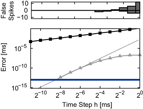
Figure 2. Integration error in the single neuron simulation (Section 2. 3.1) for different implementations of the linear neuron model as a function of the time step h. Upper panel: number of spikes incorrectly added (positive) or missed (negative) by the grid constrained implementation with respect to the spike train generated by the envelope method at the finest resolution (2−14 ms). None of the other implementations added or missed spikes. Lower panel: spike time error with respect to the reference spike train as a function of the time step h in double logarithmic representation. Non-iterative implementations: grid constrained (black squares) and cubic interpolated (gray triangles). The gray line indicates the slope expected for an error proportional to the fourth power of h. The blue line indicates the non-discrimination accuracy ϵspk = 10−13 ms.
All investigated methods reproduce all the spikes in the reference spike train for all values of h except the traditional grid constrained method. The number of added or missed spikes as a function of h is shown in the upper panel of Figure 2. One factor which can cause missed spikes is the occurrence of brief superthreshold excursions that become subthreshold again before the end of the time step. Another factor is that all excitatory and inhibitory input within a time step is treated as synchronous in the grid constrained implementation, which has a different effect on the membrane potential than when the actual arrival times of spikes is taken into consideration. This can cause both missed spikes and erroneously added spikes. Simply preserving the temporal order of incoming spikes without performing any calculations to localize outgoing spikes prevents losses and gains with respect to the reference spike train (data not shown).
As described in Section 2.2.1, a time-driven implementation can miss an outgoing spike if the superthreshold excursion of the membrane potential is of too short a duration to be detected by the V(t) ≥ Θ test at the next incoming spike or the end of the time step h. To investigate the likelihood of this occurrence, we repeat the single neuron simulation (Section 2.3.1) with the configuration Ix = 499 pA, νext = 2.71 kHz,  , and the configuration Ix = 0 pA, νext = 18.17 kHz,
  for a wide range of input rates νsn and excitatory synaptic strengths
  , whilst maintaining a constant proportion between inhibitory and excitatory synaptic strengths:
  with g = 6.25. For each configuration (Ix,νext,νsn,
 ) we perform 50 trials of 10,000 s each with the iterative time-driven implementation and record the mismatch between the number of spikes produced and the number of spikes in the reference spike train simulated with an embedded event-driven technique.
In the case that a strong subthreshold current is applied (Ix = 499 pA, νext = 2.71 kHz), the iterative time-driven implementation does not miss a single spike for any choice of (νsn, ). In the case that the subthreshold current is replaced by a corresponding Poisson input (Ix = 0 pA, νext = 18.17 kHz), spikes are occasionally missed. Figure 3 shows the proportion of spikes lost, i.e., the average (over trials) mismatch in spike number divided by the number of spikes in the reference spike train, as a function of the mean and the standard deviation of the free membrane potential (see Kuhn et al., 2004). The proportion of spikes missed is very low for all tested configurations. It does not critically depend on whether the mean free membrane potential is subthreshold, resulting in irregular, fluctuation-driven firing, or superthreshold, resulting in regular, mean-driven firing. The very low values indicate that missing a spike is a localized problem. Once a spike has been missed, the leaky integrator swiftly returns to the reference trajectory. If this were not the case, we would expect to see multiple spike mismatches once the first spike error had been made. The probability of missing a spike is greatest (2.3 × 10⁻⁴) when the input rate is low, the time step is large (1 ms in Figure 3A) and the mean membrane potential is high. This is unsurprising, as a high membrane potential is necessary for a spike to induce a brief superthreshold excursion and the combination of low input rate and large step size reduces the chances that the excursion will be detected. Simulating with a smaller time step (0.125 ms in Figure 3B) weakly decreases the proportion of missed spikes in general but has the strongest effect in the regimes where the probability of missed spikes is highest: the maximum probability of missing a spike is 4.6 × 10⁻⁵.
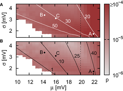
Figure 3. Proportion of false spikes generated in the single neuron simulation by the iterative time-driven implementation with respect to the spike train generated by the envelope method as a function of the mean and standard deviation of the free membrane potential. Spike trains are generated with Ix = 0 pA and νext = 18.17 kHz and the error is averaged over 50 trials of 10,000 s. Values capped at 1 × 10⁻⁴ to preserve visual clarity for lower values. (A) Simulation using a time step h = 1 ms. White contour lines indicate total input rates of 20, 30, and 50 kHz. (B) As in (A) but for h = 0.125 ms. Black contour lines indicate resulting output firing rates of 1, 10, and 40 Hz. Points A and B are chosen for more detailed analysis in Figure 4, point C indicates the statistics of the membrane potential in our standard network simulations as described in Section 2.3.2. Dashed vertical lines separate the region where the mean membrane potential is subthreshold from the region where it is superthreshold. In the white areas no measurement could be made due to extremely low or zero output rate.
To put these probabilities into context, let us consider our benchmark network of 12,600 neurons as described in Section 2.3.2. For the case that Ix = 0 pA, the total input rate is 30.8 kHz and the output rate is approximately 10 Hz. The resulting membrane potential statistics is indicated by point C in Figure 3. Due to the chaotic network dynamics, there is no way to directly determine the number of missed spikes. However, by scaling up from the measurements on the single neuron simulation, we can make a theoretical estimate of the number of spikes lost per second by using the time-driven implementation. For a time step of 1 ms, the probability of missing a spike in the single neuron is approximately 3.81 × 10⁻⁵, suggesting a loss of up to five spikes per second for the entire network. Reducing the time step to 0.125 ms reduces the single neuron spike loss probability to approximately 1.35 × 10⁻⁵, leading to a network loss of up to two spikes per second. These results suggest that when using iterative time-driven or embedded event-driven techniques, the largest time step compatible with the constraints of the neuronal system under investigation should be used.
To give better insight into the relationship between the input rate, the statistics of the membrane potential, the time step and the probability of missing a spike, we choose two input regimes to investigate in greater detail (points A and B in Figure 3).For a simulation of 1000 s we record the membrane potential and the net current at each incoming spike. For each point (I(0),V(0)), the rise time trise(I(0),V(0)) of a PSP starting from that point can be determined (see Eq. 5 in Appendix) and thus the maximum of the membrane potential V(trise). Figures 4A,B show the density of states P(I(0),V(0)) for the two chosen input regimes and the areas in state space for which V(trise) > Θ, i.e., the areas in state space which result in a membrane potential trajectory that exceeds threshold. From the density of states in these areas we can calculate the cumulative probability of trise; this is shown in Figure 4C. The smaller the rise time, the greater the probability of missing a superthreshold excursion for a given sampling rate of the membrane potential. For both input regimes, the rise times of all membrane potential excursions that can cause a threshold crossing are less than 1 ms, but the probability of very small rise times is greater for the high mean membrane potential regime shown in Figure 4A. For the low mean membrane potential regime (Figure 4B), the mean interspike interval of the incoming spike rate is smaller than the smallest rise times that occur, thus the probability of a brief superthreshold excursion occurring between two sample points is very low (2.7 × 10⁻⁵ for h = 1 ms). For the high mean membrane potential regime, the mean interspike interval of the incoming spike rate is greater than the smallest rise times that occur, thus the probability of a superthreshold excursion occurring between two sample points is greater (1.4 × 10⁻⁴). The sampling of the membrane potential due to the time step h is at a much lower rate than the sampling due to the incoming spike train, thus the effect of the time step h on the probability of missing a spike is weak as shown in Figure 3.
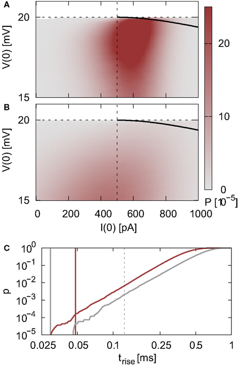
Figure 4. State density and rise times of the membrane potential excursion. (A) Density of states P(I(0),V(0)) for a neuron receiving a total input spike rate of 20.7 kHz with mean μ = 22 mV and standard deviation σ = 1.73 mV of the free membrane potential. The black edged area indicates the region in the state space where a threshold crossing will occur without additional input, V(trise) ≥ Θ. The horizontal dashed line indicates the firing threshold and the vertical dashed line indicates the minimum current that can cause a threshold crossing. (B) As in (A) but for a total input spike rate of 33.8 kHz with μ = 14.4 mV and σ = 3.39 mV. (C) Cumulative probability of trise for the states within the triangular areas (A; red, B; gray). Gray dashed vertical line indicates 0.125 ms. Red (0.048 ms) and gray (0.03 ms) vertical lines indicate the mean interspike intervals of the input firing rates in (A) and (B) respectively.
3.2 Simulation Times of Linear Neuron Model Implementations
In order to compare time-driven and event-driven implementations fairly it is necessary to show that an event-driven implementation can be successfully embedded in a globally time-driven simulation, i.e., that its performance does not depend critically on the time step h. The single neuron simulations investigated above would not necessarily help us to obtain a clear idea of the difference in performance between implementations, as the entire data can fit into the cache memory. Instead, we measure the simulation time for the test case of a moderately large recurrent network model, thus ensuring that disparities between the memory bandwidth requirements of the different implementations are included in the measurement of computational costs. Figure 5 shows the simulation time for a network simulation (Section 2.3.2) as a function of h for all the implementations of the linear benchmark neuron model described in Section 2.1.1.
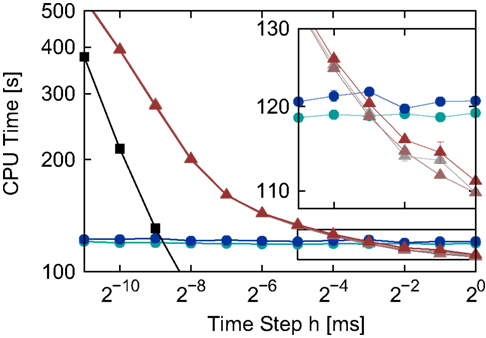
Figure 5. Simulation times for the network simulation (see 2.3.2) for the different implementations of the linear neuron model as functions of the time step h in double logarithmic representation. Time-driven implementations: grid constrained (black squares), cubic interpolated (gray triangles), Newton–Raphson (light red triangles) and bisectioning (dark red triangles). Embedded event-driven implementations: polynomial algorithm (blue circles) and the envelope algorithm (green circles). The inset shows an enlargement of the area indicated by the black rectangle; error bars show the standard deviation of the mean over five trials. Missing error bars indicate that the standard deviation is contained within the symbol size.
The simulation times of the two embedded event-driven algorithms are constant across the range of time steps tested, demonstrating that the embedding technique does not impose additional costs related to the time step h on the performance of the algorithms. Unsurprisingly, the traditional grid constrained implementation is faster than all other implementations, but its simulation times converge to those of the time-driven interpolated and iterative implementations for very small h, as was previously observed in Morrison et al. (2007). The three different spike location algorithms of the interpolating and iterative time-driven implementations yield very similar run times. The inset of Figure 5 shows that the bisectioning algorithm is slightly slower than the interpolation or Newton–Raphson techniques, but this accounts for less than 1.2% of the run time. This demonstrates that for time-driven implementations, the choice of spike location algorithms is not critical: the run time depends almost exclusively on the complexity of the operations that have to be performed for each incoming spike. Therefore, if implementing a neuron model for which straightforward Newton–Raphson is not appropriate, a more sophisticated and robust algorithm to locate the spikes can be used without fear of incurring a significant run time penalty.
The interpolated and iterative time-driven implementations are faster than the polynomial and envelope embedded event-driven implementations for large values of the time step, but due to the increase in the simulation times of the time-driven implementations with decreasing h, a cross-over occurs at around h = 2−3 ms = 0.125 ms; this is shown more clearly in the inset of Figure 5. However, as all the implementations employing iterative techniques to locate spikes achieve non-discrimination accuracy in locating a spike for all time steps h and the already small probability of missing a spike decreases only weakly with decreasing h, the choice of a small h for network simulations should not be dictated by accuracy concerns. A valid reason for reducing the time step is if it is constrained by some property of the network, for example the minimum synaptic delay. Therefore, in order to gain a better insight into which regimes are more appropriate for time-driven or event-driven simulation, we repeated the previous experiment whilst systematically varying the minimal synaptic delay by introducing one (non-functional) synaptic connection of the desired duration. As described in Section 2.2, the minimum synaptic delay determines the communication interval Tcomm, and we set the time step h = Tcomm for each value of Tcomm. Figure 6 shows the simulation times for the network simulation (Section 2.3.2) as a function of the communication interval Tcomm for all implementations of the linear neuron model employing iterative spike location algorithms.
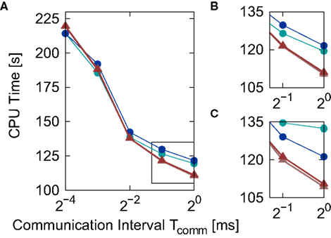
Figure 6. Simulation time for the network simulation (Section 2.3.2) for different implementations of the linear neuron model as a function of the communication interval Tcomm. (A) Simulation time for the iterative time-driven Newton–Raphson (light red triangles) and bisectioning (dark red triangles) implementations and embedded event-driven polynomial (blue circles) and envelope (green circles) implementations. (B) Enlarged view of the section indicated by the black rectangle in (A). (C) Same section as (B), but with results obtained for an alternative synaptic time constant τsyn = 5 ms. Error bars in (B,C) indicate the standard deviation of the mean over five trials. Missing error bars indicate that the standard deviation is contained within the symbol size.
Similarly to Figure 5, the iterative time-driven implementations are faster than the embedded event-driven implementations for large values of the communication interval. At Tcomm = 20 ms = 1 ms, the time-driven implementations are 10% faster than the embedded event-driven implementations. As the communication interval decreases, all simulation times increase. This is because the cache efficiency advantage of integrating a neuron’s incoming spikes for a complete communication interval in only one visit from the scheduling algorithm diminishes as the communication interval decreases, which affects all implementations in the same manner. For small communication intervals the simulation times converge, with a slight speed advantage to the embedded event-driven implementations. However, the introduction of the communication interval optimization only guarantees a performance advantage to event-driven methods if at least one spike per communication delay is expected, as discussed in Section 2.2.2. At a communication interval of 2−4 ms = 0.0625 ms, the communication step is smaller than the interspike interval of the incoming spike train each neuron in the network sees (1/15.31 kHz = 0.0653 ms). This means that the time-driven scheduling algorithm visits the neuron more often than an event-driven scheduling algorithm would, and so could be disadvantaging the performance of the event-driven methods. In summary, the time-driven implementations are either significantly faster than the event-driven methods or are similarly fast, depending on the communication interval. As the time-driven approach is more general, this suggests it should be the preferred technique for simulations in which high accuracy for the spike timing is required. If the interspike interval of the incoming spike train is greater than the minimal synaptic delay in the network, event-driven techniques may be more advantageous.
The envelope method of D’Haene et al. (2009) is faster than the polynomial approach of Brette (2007) for the parameters chosen, however parameters can be found that reverse the relationship. Figure 6C shows the same section as Figure 6B but for a network simulation with the following deviations from the parameters given in Section 2.3.2:  ,
,  νext = 3.498 kHz, and τsyn = 5 ms. The increased synaptic time constant reduces the order of the polynomial mapping of the membrane potential to 2, which increases the efficiency of the algorithm presented in Brette (2007) and summarized in Section 2.2.2.1.
3.3 Efficiency of Linear Neuron Model Implementations
In Section 3.1 we investigated the accuracy of time-driven and event-driven implementations of the linear benchmark neuron in single neuron simulations. In Section 3.2 we measured the simulation time for the various implementations in the test case of a recurrent network model. However, in order to choose between candidate implementations of a neuron model for a specific scientific question, a researcher needs to know which implementation will achieve a given accuracy goal for the lowest run time cost. We therefore follow the definition developed in Morrison et al. (2007), i.e., the efficiency of a neuron model implementation is the run time cost to achieve a particular accuracy goal, rather than the run time costs at a particular time step. As the dynamics of our benchmark network model exhibits chaotic behavior (Brunel, 2000), it is not possible to define a single reference spike train. However, although no accuracy measurement can be made for the recurrent network model, the run time costs measured give a fair reflection of the costs of using a particular neuron model implementation. We therefore conjoin the run time costs measured for the recurrent network with an accuracy goal defined as the integration error obtained for a single neuron simulation with the same input statistics. In other words, we combine the information displayed in Figures 2 and 5 to derive the run time cost as a function of the single neuron integration error, eliminating the time step h. The results of this analysis are shown in Figure 7A; Figure 7B shows an enlarged view of the section indicated by the black rectangle to illustrate more clearly the relationships between the various implementations that obtain non-discrimination accuracy at all time steps.
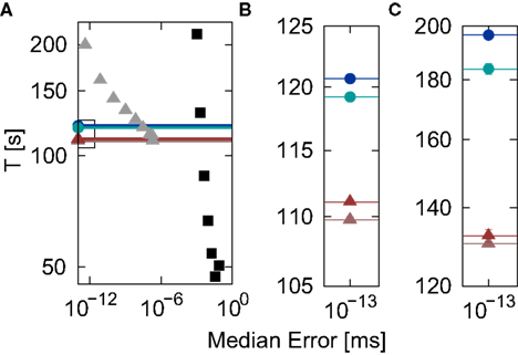
Figure 7. Simulation time for the network simulation (Section 2.3.2) as a function of the integration error in the single neuron simulation (Section 2.3.1) for different implementations of the linear neuron model. (A) Simulation time in double logarithmic representation for the time-driven implementations: grid constrained (black squares), cubic interpolated (gray triangles), Newton–Raphson (light red triangles), bisectioning (dark red triangles) and the embedded event-driven implementations: polynomial (green circles), envelope (blue circles). Implementations that achieve non-discrimination accuracy at all time steps are represented by their simulation times for h = 1 ms and drawn as a single marker and a line for greater visual clarity. (B) Enlarged view of the section indicated by the black rectangle in (A). (C) As in (B) but for Ix = 0 and νext = 18.17 kHz.
The analysis demonstrates that an accuracy goal of 10−13 can be most efficiently obtained by a time-driven implementation employing iterative spike location techniques. The Newton–Raphson technique proves to be marginally more efficient than the bisectioning technique. For the parameters used, the analysis also confirms a central result of D’Haene et al. (2009), i.e., that their envelope method is more efficient than the polynomial method of Brette (2007), although parameters can be found that are preferential for the Brette (2007) approach (see Figure 6C). The difference seen in efficiency between the two embedded event-driven methods (1.2%) is substantially smaller than that between the more efficient of the embedded event-driven implementations and the more efficient of the iterative time-driven implementations that we propose (7.9%).
Although this efficiency advantage of the time-driven implementation is relatively modest, it was determined for a network simulation that is parameterized to provide a best-case for the embedded event-driven implementations in terms of speed, and the implementations themselves are reduced to their simplest and least general cases (Section 2.2.2.1 and 2.2.2.2), whereas the time-driven implementation is not optimized for the specific neuron model. Figure 7C shows the results of a network simulation in which the subthreshold input current is replaced by an external Poisson input of rate νext = 18.17 kHz and strength  . The greater complexity of the embedded event-driven algorithms with respect to the treatment of incoming spikes results in a 29.0% difference between the more efficient of the embedded event-driven implementations and the more efficient of the iterative time-driven implementations. Although there is a small probability of the time-driven implementation missing a spike (see Figure 3), this event did not occur.
If the scientific question under investigation requires a lesser degree of precision, a non-iterative method can be more appropriate. Figure 7A shows that if median errors greater than 10−2 ms are acceptable, the grid constrained implementation remains the method of choice.
To demonstrate that the results obtained above are robust with respect to the total rate of incoming spikes a neuron implementation processes and the rate of outgoing spikes it generates, we performed a series of network simulations in which the input and output rates can be cleanly disentangled (see 2.3.3). Figure 8 shows the results of this analysis. The time-driven implementation with iterative spike location is faster than the embedded event-driven algorithm employing the envelope method of D’Haene et al. (2009) for all tested input and output rates (see Figure 8A). The time-driven method becomes comparatively more advantageous for increasing input and output rates. The dependence on the input rate can be explained as follows. As already demonstrated in Figure 5, the run time depends not on the computational expense of the method used to locate the spikes but on the expense of the operations performed on receiving each input spike. The iterative time-driven and the embedded event-driven implementations have the common cost of propagating the neuron state from one input spike to the next. Beyond that cost, the minimal operation performed by a time-driven implementation is to check for the superthreshold condition, which is less expensive than the minimal operation performed by an event-driven implementation, namely performing a prediction of whether the neuron can fire in the future without additional input. Therefore as the number of incoming spikes increases, so too does the comparative advantage of the time-driven approach, as can be seen in Figure 8B. The dependence on the output rate is due to the number of times the spike location method is called. In the time-driven implementations, the spike location method is only carried out if a superthreshold condition was detected, i.e., when an outgoing spike should definitely be generated. In contrast, an event-driven method must at least start the search algorithm every time the spike prediction algorithm indicates that a spike is possible without further input. In many cases, the spike location algorithm will be aborted or invalidated by the arrival of the next incoming spike. In a high rate regime, positive predictions are more common than in a low rate regime, so the complexity of the event-driven algorithm is also dependent on the output rate, whereas the complexity of the time-driven implementations are essentially independent of it. The dependence of the run time on the output rate is demonstrated in Figure 8C. The computation time of the embedded event-driven implementation increases linearly with the output rate whereas the computation time of the time-driven implementation remains roughly constant. The statistics of the output spike train, i.e., irregular, fluctuation-driven firing when the mean free membrane potential is subthreshold, and regular, mean-driven firing in the superthreshold regime, does not affect the comparative advantage of the time-driven implementation.
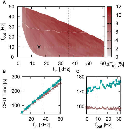
Figure 8. Comparison of performance between the time-driven implementation with iterative (Newton–Raphson) spike location with respect to the embedded event-driven implementation employing the envelope algorithm of D’Haene et al. (2009). (A) Performance gain (Section 2.3.3) of the iterative time-driven implementation with respect to the embedded event-driven implementation as a function of input and output rates. Color indicates the relative decrease in simulation time obtained by using the time-driven iterative implementation for a network simulation with the given total input (horizontal axis) and output (vertical axis, different scale) rates. Dotted lines indicate the cross-sections taken for (B) and (C). The black X indicates the input and output rates of the network used for Figures 6 and 7. The white contour line separates the region in which the mean free membrane potential is superthreshold (above) from the region in which it is subthreshold. White regions indicate that no measurements were made. (B) Simulation time for the iterative time-driven (light red triangles) and the embedded event-driven (green circles) implementations as a function of the input rate at constant output rate (10 Hz). (C) As in (B) but simulation time shown as a function of the output rate at constant input rate (36.3 kHz). The dotted lines in (B) and (C) indicate the cross-sections taken for (C) and (B)respectively.
The range of output rates generated by the method used to locate appropriate parameter configurations (Section 2.3.3) is dependent on the input rate, resulting in the white areas where no measurements could be made. In particular, it is difficult in this framework to produce low rate output when the input rate is very low. As the comparative advantage of the time-driven implementation decreases with decreasing input and output rates, event-driven methods may prove advantageous for scientific questions where sparse activity can be assumed, either due to low firing rates or low connectivity.
3.4 Performance of the Non-Linear Neuron Model
To demonstrate the generality of our approach we apply it to the non-linear AdEx model (Brette and Gerstner, 2005) described in Section 2.1.2. The adaptation of our technique to a non-linear model is given in Section 2.2.1: a standard adaptive ODE solver is used to integrate the dynamics between incoming spikes. If the superthreshold condition is detected after an integration step, a linear interpolation is performed across the integration step to locate the spike. To measure accuracy, we define the reference spike train to be that generated by our linearly interpolating technique simulated at the finest resolution (h = 2−14 ms) and with the lowest absolute maximum local solver error (ϵabs = 10−12). Reducing ϵabs further than this does not result in better accuracy, i.e., the median spike error saturates at 10−12 ms for any choice of ϵabs ≤ 10−12 for the reference and test spike trains (data not shown). We will therefore consider 10−12 ms to be the best achievable accuracy for this model. The results of the comparison of our technique with a standard grid constrained implementation are shown in Figure 9 (see Section 2.4 for the details of the protocol).
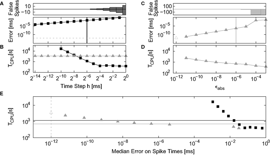
Figure 9. Accuracy, simulation time, and efficiency for the grid constrained (black squares) and linear interpolating (gray triangles) implementations of the non-linear neuron model. Accuracy is determined with respect to the reference spike train generated by the linear interpolating implementation at the finest resolution (h = 2−14 ms) and lowest absolute maximum local solver error (ϵabs = 10−12). (A) Lower panel: integration error in a single neuron simulation as a function of the time step h in double logarithmic representation. For the grid constrained implementation ϵabs = 10−6. The linear interpolating implementation with ϵabs = 10−12 generates identical spike trains to the reference train for all h; the error is therefore represented by the gray dashed line indicating the best achievable accuracy, 10−12 ms. For h > 2−6 ms (vertical black line) the grid constrained implementation misses or adds spikes with respect to the reference spike train. Upper panel: number of spikes incorrectly added (positive) or missed (negative) by the grid constrained implementation with respect to the reference spike train. (B) Simulation time for the network simulation as a function of the time step h in double logarithmic representation, ϵabs as in (A). (C) Lower panel: integration error of the linear interpolating implementation in a single neuron simulation at h = 20 ms as a function of the solver maximum error ϵabs in double logarithmic representation. Error for ϵabs = 10−12 (open triangle) represented by the best achievable accuracy, 10−12 ms. For ϵabs > 10−6 (vertical gray line) spikes are missed. Upper panel: number of spikes missed with respect to the reference spike train. (D) Simulation time for the network simulation as a function of the solver error. (E) Simulation time for the network simulation as a function of the integration error in the single neuron simulation in double logarithmic representation. The data for the grid constrained implementation are consolidated from (A,B), eliminating h; the data for the linear interpolating implementation are consolidated from (C,D), eliminating ϵabs. Horizontal lines (h = 2−6 ms: black, ϵabs = 10−6: gray) correspond to the vertical lines in (B) and (D). Vertical gray dashed line corresponds to the horizontal gray dashed line in (A).
The accuracy of the grid constrained implementation in the single neuron simulation improves gradually with decreasing time step h. For h ≤ 2−6 ms (black vertical line in the lower panel of Figure 9A) the reference spike train is faithfully reproduced, i.e., there are no missed or added spikes. For smaller time steps, the error in locating the individual spike times decreases further. The simulation time for the network simulation when using the grid constrained implementation (Figure 9B) remains constant for h ≥ 2−4 ms and then increases steadily with decreasing h. These results were obtained with the absolute maximum local error of the solver ϵabs set to 10−6. Reducing ϵabs further does not improve the accuracy of the integration but does increase the run time, whereas increasing ϵabs leads to unacceptably high numbers of missed spikes with respect to the reference spike train (data not shown).
In contrast, the linear interpolating implementation generates spike trains identical to the reference spike train in the single neuron simulation for all values of h. As no error can be defined in this case, the best achievable accuracy of 10−12 ms is shown as a visual guide in Figure 9A. Similarly, the run time performance for the network simulation was constant for all values of h (Figure 9B). These results were obtained with the absolute maximum local error of the solver ϵabs set to 10−12. To investigate the role of ϵabs we repeated the single neuron and network simulations for the linear interpolating implementation for h = 20 ms whilst systematically varying ϵabs. The results are shown in Figures 9C,D. As ϵabs increases the integration error in the single neuron error increases steadily but the simulation time for the network simulation decreases steadily. For ϵabs ≤ 10−6 (gray vertical line in the lower panel of Figure 9C) the reference spike train is faithfully reproduced; above this value many spikes are missed with respect to the reference spike train.
To compare the efficiency of the two implementations of the non-linear neuron model, we once again plot the simulation time for the network simulation as a function of the integration error in the single neuron simulation, eliminating h as the independent variable for the grid constrained implementation, and ϵabs for the linear interpolating implementation (Figure 9E). The horizontal lines, corresponding to the vertical lines in Figures 9A,C, indicate the least expensive simulation in terms of run time for which the reference spike train in the single neuron simulation is reliably reproduced. The gray line runs below the black line, which demonstrates that our technique is more efficient in terms of generating reliable spike trains than the standard grid constrained implementation. Moreover, the marker bisected by the gray line lies to the left of the marker bisected by the black line, which shows that the accuracy of the individual spikes is better using the linear interpolating implementation at ϵabs = 10−6 than using the grid constrained implementation at h = 2−6 ms. Improved accuracy for the spike timing is achievable for the linear interpolating implementation at the cost of increasing the run time by reducing the maximum local error of the solver ϵabs.
4 Discussion
We have compared several different methods of accurately calculating the spike times of the linear integrate-and-fire neuron model with exponentially decaying synaptic currents, for which the next spike time cannot be expressed in closed form. In order to evaluate the performance of different approaches, it was necessary to implement all techniques within the same simulation environment. Initially, this may seem paradoxical – how can an event-driven method be fairly implemented in a globally time-driven simulation environment? However, we have taken great care to ensure that the event-driven methods of Brette (2007) and D’Haene et al. (2009) were embedded, parameterized and stimulated in such a way as to meet or surpass their efficiency in a purely event-driven environment.
Let us first consider their implementation (Section 2.2.2). In our versions, the event-driven methods do not perform any additional calculations at the grid points defined by the time step h, and so the run times of these implementations are independent of h (see Figure 5). The run time is dependent on the communication interval Tcomm, however the introduction of this variable is an optimization that improves the performance of all implementations. By allowing the greatest possible number of operations for a given neuron instance to be performed sequentially, the cache efficiency is improved and the run time is lowered. This advantage holds as long as at least one input event per communication interval is expected. The globally time-driven simulation algorithm also scales well when distributing an application over multiple machines (Morrison et al., 2005); communicating precise spike times only increases the size of the packets by a constant factor, but does not increase the frequency or overhead of communication (Morrison et al., 2007). Distributing a globally event-driven simulation algorithm requires additional mechanisms to maintain consistency between the event queues on each machine (Lytton and Hines, 2005; Migliore et al., 2006). The temporal separation of the invocation of spike prediction and the spike location algorithms represents another optimization that can only be realized in a time-driven environment. This feature reduces the search costs that occur in an event-driven environment in the common case that subsequent input would alter or cancel the spike time that has been calculated for a neuron. Due to the use of intermediate variables to store the state of the spike location algorithm, the only additional costs that accrue to the event-driven methods as a result of being embedded in a time-driven scheduling algorithm is an additional function call at the end of each communication interval. We assert that the cost of this function call is more than compensated for by the time-driven optimizations described above.
Secondly, let us consider the parameterization and stimulation. By using identical time constants for all synaptic currents and choosing the time constant of the membrane potential to be an integer multiple of the synaptic time constant, we simplify the prediction and spike location algorithms of both the polynomial method of Brette (2007) and the envelope method of D’Haene et al. (2009) to their best cases. The high subthreshold current (Section 2.1.1) which drives the neurons to just below their firing threshold reduces the number of inputs a neuron must receive in order to fire. This is advantageous for the event-driven techniques, as they incur higher costs for an incoming event than a time-driven technique. An even higher current cannot be applied due to the limitations of the Brette (2007) algorithm. Finally, in the case of the event-driven implementations, the timing of events in the Poissonian input spike trains was defined with respect to a Tcomm basis rather than a h basis to avoid unnecessary numerical conversions. To enable other researchers to perform their own experiments, we are making a NEST module available for download from www.nest-initiative.org that contains all used implementations.
Despite all the care taken to enhance the efficiency of the event-driven implementations of the linear integrate-and-fire model, they proved to be less efficient for all tested input and output rates than the time-driven implementations based on the “canonical” technique first presented in Morrison et al. (2007) but incorporating iterative algorithms to locate outgoing spikes. By replacing the subthreshold input current with a corresponding Poisson spike train, the network simulation is less specifically designed to favor the event-driven approach and the comparative speed advantage of the time-driven technique is substantially greater. The better performance of the time-driven implementation is because the run time depends on the cost of the operations performed for each incoming spike and not for each outgoing spike. This can be clearly seen by comparing the run times for the various time-driven implementations in Figure 5: the grid constrained implementation, which merely increments the weight in a buffer for each incoming event, is the fastest. All other time-driven implementations have essentially the same speed, despite different complexities of the spike location algorithm. Time-driven implementations are faster than event-driven implementations at large time steps because checking for a superthreshold condition at each incoming spike is cheaper than the corresponding operations in an event-driven scheme, i.e., performing a spike prediction algorithm and initiating a search algorithm if the prediction is positive. A time-driven implementation can miss spikes due to brief superthreshold excursions of the membrane potential. We have shown that the probability is small for a wide range of input and output rates, with a maximum in the order of 10−4 for a time step of 1 ms; in future work we will investigate whether the probability of missing a spike can be reduced still further.
In addition to the detection of threshold crossings, another component determining the accuracy of the solution is the accuracy at which the subthreshold dynamics is propagated in time. An obvious constraint is the number of bits used to represent the floating point values; if available, the accuracy can be increased by replacing the double representation with quad representation. Independent of the representation, care should be taken to select appropriate library functions for computing exponentials and to sort terms with respect to their magnitudes (Morrison et al., 2007). Moreover, instead of expressing the system state in the natural variables of potential and current suggested by the biophysics, it can be transformed to obtain a better conditioned time-evolution operator (Deuflhard and Bornemann, 2010). An example of such a transformation in the context of neuronal dynamics is provided in Appendix B of Guerrero-Rivera et al. (2006), although the motivation for that study was to reduce the number of multiplications rather than to increase the accuracy.
Through our experiments we were able to establish categories of atypical situations in which event-driven simulation may prove more efficient. If even a very low probability of missing a spike is unacceptable for the scientific question at hand, an event-driven algorithm provides the required guarantee for the linear neuron model we investigated. By investigating a wide range of input and output rates (see Figure 8) we determined that the comparative speed advantage of the time-driven implementation decreases with decreasing input and output rate. A further example of a situation in which event-driven simulation may be more efficient is therefore the limit of extremely low input and output rates beyond our tested range. However, such a simulation is likely to run very quickly regardless of which approach is used, and so the decision of which approach to take is not as crucial as for a network of the same size with higher input and output rates. As the iterative time-driven implementation attains non-discrimination accuracy at all time steps given correct spike detection, the size of the time step is more constrained by features of the neural system under investigation than by accuracy requirements. The most likely reason for requiring a small time step is that the synaptic delays are very short, as the minimum synaptic delay constrains the time step. If the activity of the network and the minimum synaptic delay are such that less than one incoming spike per communication interval can be expected, then an event-driven simulation may be more efficient (see Figure 6). For example, this situation could arise if gap junctions are considered, which have a much lower transmission delay than chemical synapses. A final example depends on the specific neuron model. The envelope method of D’Haene et al. (2009) can integrate neuron models with a large number of different synaptic time constants. A thorough investigation of the time-driven performance of such models lies outside the scope of this manuscript. Furthermore, our investigations have dealt with neuron models with non-invertible dynamics, such that the time of the next spike cannot be expressed in closed form. For neuron models with invertible dynamics [e.g., the Theta-neuron model (Ermentrout and Kopell, 1986; McKennoch et al., 2009) and the Mirollo–Strogatz model (Mirollo and Strogatz, 1990)] the costs of future spike location can be expected to be lower, thus expanding the regimes in which event-driven simulation is more efficient.
Similarly, there is also a large class of network models for which time-driven simulation without iterative spike location is more appropriate. As demonstrated in Figure 7, if a large error in the timing of spikes is acceptable, a grid constrained implementation is substantially faster. For networks with chaotic dynamics such as those used here to measure the computational costs of the various neuron model implementations, it is not possible to define a “correct” reference spike train to which measurements converge. Even the smallest difference in the computer representation of spike times or in the implementation of mathematical functions will lead to divergent results in a short time. In such cases, the former concept of spike time error is irrelevant. As long as no mesoscopic effects such as artificial synchronization emerge, there is no advantage to using an implementation with a high degree of accuracy in spike location instead of a faster, less accurate implementation. If such mesoscopic effects occur, simple, low cost techniques such as performing the neuron reset off-grid may already be sufficient to suppress the artifactual behavior (Hansel et al., 1998; see also the elaboration in Morrison et al., 2007).
In addition to its greater efficiency for neuron models with non-invertible dynamics, our approach has the major advantage of generality. The algorithms of Brette (2007) and D’Haene et al. (2009) provide elegant solutions for a specific linear neuron model, but require additional constraints to operate at their best [the polynomial algorithm of Brette (2007) is particularly vulnerable to the choice of neuron parameters]. In contrast, our technique can be applied to any neuron model in which a superthreshold (or analog) condition can be identified and in any network model incorporating transmission delays between neurons.
To demonstrate this generality, we applied our method to the non-linear AdEx neuron model of Brette and Gerstner (2005). The AdEx model is fundamentally different from the integrate-and-fire model, which essentially eliminates the possibility of missing a spike. In the integrate-and-fire model a spike is generated when the membrane potential passes the threshold value from below. As the membrane potential may stay above threshold only for a short time, integration algorithms which only calculate the membrane potential at specific points may fail to detect the suprathreshold value and consequently fail to generate a spike. In the AdEx model, the differential equation governing the membrane potential rapidly drives the membrane potential to large values once the threshold Vth is passed. The spike time is determined by the membrane potential passing Vpeak several millivolts above Vth. If a numerical solver integrates the differential equation with sufficient accuracy, it cannot fail to detect the generation of a spike because the membrane potential just continues to increase after crossing the threshold Vth. The introduction of Vpeak enables spike generation to be distinguished from cases where a suprathreshold membrane potential is pushed below threshold again by further inhibitory input. For a sufficiently large choice of Vpeak, an initiated spike cannot be canceled by inhibition due to the rapid increase of the membrane potential. Consequently, the precise timing of spikes depends weakly on the choice of Vpeak but the number of spikes detected does not.
We showed that when our technique is applied to the non-linear AdEx model, the generated spike trains converge to a reference spike train as the maximum local error of the adaptive solver is reduced. Additionally, our technique achieves a reliable reproduction of the reference spike train with a greater accuracy on the individual spike times at a lower computational cost than a standard grid constrained implementation (see Figure 9). A specific event-driven algorithm for the AdEx neuron model is not known. However, with current technology the model dynamics could be solved by provisionally stepping forward in time, with at least the costs of our technique, plus the additional costs of rewinding the dynamics if new events arrive that change the provisional solution (Lytton and Hines, 2005). The clear accuracy and speed advantage of our technique suggests that it should be considered the standard integration technique for the AdEx model when accurate spike times are required.
Our intention in this study was to address the common perception that time-driven approaches cannot reach the high degree of precision obtained by event-driven approaches and so we restricted our analysis to these classes. In future work, we will extend the analysis to address the potential advantages of alternative methods of integration, such as the novel and promising voltage-stepping technique proposed by Zheng et al. (2009). Another alternative is represented by analog neuromorphic hardware such as that developed within the EU FACETS project, which emulates the differential equations of the neuron model by analog electrical circuits (Schemmel et al., 2008; Bruederle et al., 2010). The detection of a threshold crossing is bounded only by the physical constraints of the reaction time of the comparator element continuously monitoring the membrane potential. As in the case of simulation on digital computers, the explosive dynamics of the AdEx model can be exploited to reduce the probability of missing a spike even further than in the case of the integrate-and-fire model. For simulations on digital computers, our results on linear and non-linear neuron models demonstrate that our technique exhibits greater efficiency and generality than event-driven techniques, except in the special cases described above, such as extremely low rates or when no spike may be missed. We therefore conclude that when the accuracy of spike times is critical, our iterative time-driven approach should be the first method to try; a specialized, event-driven implementation should only be developed if the time-driven approach yields unsatisfactory results.
Conflict of Interest Statement
The authors declare that the research was conducted in the absence of any commercial or financial relationships that could be construed as a potential conflict of interest.
Acknowledgments
Partially funded by DIP F1.2, BMBF Grant 01GQ0420 to BCCN Freiburg, EU Grant 15879 (FACETS), Helmholtz Alliance on Systems Biology (Germany), and Next-Generation Supercomputer Project of MEXT (Japan). We are grateful to our colleagues in the NEST Initiative and to Bernd Wiebelt and Michael Denker for help with the high performance computing facilities at the BCCN Freiburg and the Laboratory for Computational Neurophysics, RIKEN Brain Science Institute. The authors would like to thank H. E. Plesser and C. Trengove for their comments on an earlier version of this manuscript.
References
Brette, R. (2007). Exact simulation of integrate-and-fire models with exponential currents. Neural Comput. 19, 2604–2609.
Brette, R., and Gerstner, W. (2005). Adaptive exponential integrate-and-fire model as an effective description of neuronal activity. J. Neurophysiol. 94, 3637–3642.
Brette, R., Rudolph, M., Carnevale, T., Hines, M., Beeman, D., Bower, J. M., Diesmann, M., Morrison, A., Goodman, P. H., Harris, F. C. Jr., Zirpe, M., Natschläger, T., Pecevski, D., Ermentrout, B., Djurfeldt, M., Lansner, A., Rochel, O., Vieville, T., Muller, E., Davison, A. P., El Boustani, S., and Destexhe, A. (2007). Simulation of networks of spiking neurons: a review of tools and strategies. J. Comput. Neurosci. 23, 349–398.
Bruederle, D., Bill, J., Kaplan, B., Kremkow, J., Meier, K., Mueller, E., and Schemmel, J. (2010). “Simulator-like exploration of cortical network architectures with a mixed-signal vlsi system,” in Proceedings of the 2010 IEEE International Symposium on Circuits and Systems, Paris, France.
Brunel, N. (2000). Dynamics of sparsely connected networks of excitatory and inhibitory spiking neurons. J. Comput. Neurosci. 8, 183–208.
Deuflhard, P., and Bornemann, F. (2010). Scientific Computing with Ordinary Differential Equations. New York: Springer.
D’Haene, M., and Schrauwen, B. (2010). Fast and exact simulation methods applied on a broad range of neuron models. Neural Comput. 22, 1468–1472.
D’Haene, M., Schrauwen, B., Van Campenhout, J., and Stroobandt, D. (2009). Accelerating event-driven simulation of spiking neurons with multiple synaptic time constants. Neural Comput. 21, 1068–1099.
Diesmann, M., Hanuschkin, A., Kunkel, S., Helias, M., and Morrison, A. (2008). The performance of solvers for integrate-and-fire models with exact spike timing. Front. Neuroinform. Conference Abstract: Neuroinformatics 2008. doi: 10.3389/conf.neuro.11.2008.01.014.
Eppler, J. M., Helias, M., Muller, E., Diesmann, M., and Gewaltig, M. (2009). PyNEST: a convenient interface to the NEST simulator. Front. Neuroinform. 2:12. doi:10.3389/neuro.11.012.2008.
Ermentrout, G. B., and Kopell, N. (1986). Parabolic bursting in an excitable system coupled with a slow oscillation. SIAM J. Appl. Math. 46, 233–253.
FACETS. (2009). Fast analog computing with emergent transient states, project homepage. Available at: http://www.facets-project.org.
Galassi, M., Davies, J., Theiler, J., Gough, B., Jungman, G., Booth, M., and Rossi, F. (2006). GNU Scientific Library Reference Manual, 2nd Edn. Network Theory Limited. Bristol: UK.
Gerstner, W., and Brette, R. (2009). Adaptive exponential integrate-and-fire model. Scholarpedia 4, 8427.
Guerrero-Rivera, R., Morrison, A., Diesmann, M., and Pearce, T. C. (2006). Programmable logic construction kits for hyper real-time neuronal modeling. Neural Comput. 18, 2651–2679.
Hansel, D., Mato, G., Meunier, C., and Neltner, L. (1998). On numerical simulations of integrate-and-fire neural networks. Neural Comput. 10, 467–483.
Hanuschkin, A., Kunkel, S., Helias, M., Morrison, A., and Diesmann, M. (2008). Comparison of methods to calculate exact spike times in integrate-and-fire neurons with exponential currents. BMC Neurosci. 9(Suppl. 1), P131.
Kuhn, A., Aertsen, A., and Rotter, S. (2004). Neuronal integration of synaptic input in the fluctuation-driven regime. J. Neurosci. 24, 2345–2356.
Kumar, A., Schrader, S., Aertsen, A., and Rotter, S. (2008). The high- conductance state of cortical networks. Neural Comput. 20, 1–43.
Kunkel, S., Hanuschkin, A., Helias, M., Morrison, A., and Diesmann, M. (2009). Time-driven simulation as an efficient approach to detecting threshold crossings in precisely spiking neuronal network models, in Proceedings of the Eighth Göttingen Meeting of the German Neuroscience Society, T26-7B.
Lytton, W. W., and Hines, M. L. (2005). Independent variable time-step integration of individual neurons for network simulations. Neural Comput. 17, 903–921.
McKennoch, S., Voegtlin, T., and Bushnell, L. (2009). Spike-timing error backpropagation in theta neuron networks. Neural Comput. 21, 9–45.
Migliore, M., Cannia, C., Lytton, W. W., Markram, H., and Hines, M. (2006). Parallel network simulations with NEURON. J. Comput. Neurosci. 21, 119–223.
Mihalas, S., and Niebur, E. (2010). A generalized linear integrate-and-fire neural model produces diverse spiking behaviors. Neural Comput. 21, 704–718.
Mirollo, R. E., and Strogatz, S. H. (1990). Synchronization of pulse-coupled biological oscillators. J. Appl. Math. 50, 1645–1662.
Morrison, A., and Diesmann, M. (2008). “Maintaining causality in discrete time neuronal network simulations,” in Lectures in Supercomputational Neuroscience: Dynamics in Complex Brain Networks, Understanding Complex Systems, eds P. beim Graben, C. Zhou, M. Thiel, and J. Kurths (Berlin: Springer), 267–278.
Morrison, A., Mehring, C., Geisel, T., Aertsen, A., and Diesmann, M. (2005). Advancing the boundaries of high connectivity network simulation with distributed computing. Neural Comput. 17, 1776–1801.
Morrison, A., Straube, S., Plesser, H. E., and Diesmann, M. (2007). Exact subthreshold integration with continuous spike times in discrete time neural network simulations. Neural Comput. 19, 47–79.
Naud, R., Marcille, N., Clopath, C., and Gerstner, W. (2008). Firing patterns in the adaptive exponential integrate-and-fire model. Biol. Cybern. 99, 335–347.
Plesser, H. E., and Diesmann, M. (2009). Simplicity and efficiency of integrate-and-fire neuron models. Neural Comput. 21, 353–359.
Plesser, H. E., Eppler, J. M., Morrison, A., Diesmann, M., and Gewaltig, M.-O. (2007). “Efficient parallel simulation of large-scale neuronal networks on clusters of multiprocessor computers,” in Euro-Par 2007: Parallel Processing, Vol. 4641, Lecture Notes in Computer Science, eds A.-M. Kermarrec, L. Bougé, and T. Priol (Berlin: Springer-Verlag), 672–681.
Press, W. H., Teukolsky, S. A., Vetterling, W. T., and Flannery, B. P. (1992). Numerical Recipes in C, 2nd Edn. Cambridge: Cambridge University Press.
Rotter, S., and Diesmann, M. (1999). Exact digital simulation of time-invariant linear systems with applications to neuronal modeling. Biol. Cybern. 81, 381–402.
Schemmel, J., Fieres, J., and Meier, K. (2008). “Wafer-scale integration of analog neural networks,” in Proceedings IJCNN2008. Piscataway, NJ: IEEE Press.
Shelley, M. J., and Tao, L. (2001). Efficient and accurate time-stepping schemes for integrate-and-fire neuronal networks. J. Comput. Neurosci. 11, 111–119.
van Elburg, R. A. J., and van Ooyen, A. (2009). Generalization of the event-based Carnevale–Hines integration scheme for integrate-and-fire models. Neural Comput. 21, 1913–1930.
Keywords: precise spike times, accuracy, time driven, event driven, non-linear neuron models
Citation: Hanuschkin A, Kunkel S, Helias M, Morrison A and Diesmann M (2010) A general and efficient method for incorporating precise spike times in globally time-driven simulations. Front. Neuroinform. 4:113. doi: 10.3389/fninf.2010.00113
Received: 03 December 2009;
Paper pending published: 13 January 2010;
Accepted: 11 August 2010;
Published online: 05 October 2010.
Edited by:
Anders Lansner, Royal Institute of Technology, SwedenReviewed by:
Anthony Burkitt, The University of Melbourne, AustraliaDominique Martinez, LORIA, France
Copyright: © 2010 Hanuschkin, Kunkel, Helias, Morrison and Diesmann. This is an open-access article subject to an exclusive license agreement between the authors and the Frontiers Research Foundation, which permits unrestricted use, distribution, and reproduction in any medium, provided the original authors and source are credited.
*Correspondence: Alexander Hanuschkin and Susanne Kunkel, Functional Neural Circuits Group, Faculty of Biology, Albert-Ludwig University of Freiburg, Freiburg im Breisgau, Germany. e-mail: hanuschkin@bcf.uni-freiburg.de; kunkel@bcf.uni-freiburg.de